PDF reweighting in the Hessian matrix approach

A large part of the present high-energy collider physics depends, in one way or another, on the knowledge of the parton distribution functions (PDFs). The use of PDFs leans on a cornerstone theorem of Quantum Chromo Dynamics (QCD), the collinear factorization [1, 2]. Although it can be formally proven only for the most simple cases, it is often assumed to work in general. Ultimately, it is the agreement with the experimental data that decides whether such an assumption is valid.

The PDFs are traditionally determined in global analyses [3, 4, 5, 6] finding the parametrization that can optimally reproduce a variety of experimental data. This is a complex procedure requiring the ability to efficiently solve the parton evolution equations and to calculate higher-order QCD cross-sections. Nontrivial issues are also the actual way of finding the best fit and quantifying its uncertainties. Although various PDF parametrizations are publicly available for a general user, for a long period of time it was difficult for e.g. an experimental collaboration to understand what would be the implications of their measurements in the context of a global PDF fit. For example, although a given measurement would be known to be most sensitive to, say, the up quark distribution, some other data in a global fit may already provide the up quarks with more stringent constraints, and the real advantage of the measurement would be due to a sub-leading contribution, say, from the strange quarks.

The Bayesian reweighting technique, first introduced in [7] and later on elaborated by the Neural Network PDF (NNPDF) collaboration [8, 9], provides a way of addressing the consistency and quantitative effects of a new experimental evidence in terms of PDF fits. In essence, the underlying probability distribution, represented in the NNPDF philosophy [6] by an ensemble ($\sim 1000$) of PDF replicas, is updated by assigning each replica a certain weight based on the new data. This method has become an increasingly popular way to estimate the effects of e.g. new LHC measurements [10, 11, 12, 13, 14, 15, 16]. The drawback is that it has been proven to work only in conjunction with the NNPDF fits while the majority of the existing PDF fits use a rather different way of quantifying the PDFs and their uncertainties. Along with the best fit found by $\chi^{2}$ minimization, they provide a collection ($\sim 50$) of Hessian error sets [17] that quantify the neighborhood of the central fit within a certain confidence criterion $\Delta\chi^{2}$. An extension of the Bayesian reweighting technique to this particular case was suggested in [18], and has thereafter been used in some occasions [11, 19, 20]. However, a recent study [21] revealed clear deviations when comparing the results from reweighting to the ones obtained by a direct fit, indicating that the proposed generalization is not accurate.

Here we take a different strategy. Based on the ideas presented in Ref. [22], our principal goal is to show how a general user can directly study the consistency and consequences of a new data set within an existing set of PDFs that comes with the Hessian error sets without having to lean on the Bayesian techniques. The method naturally incorporates the confidence criterion $\Delta\chi^{2}$ defined in the original fit and, by considering a simple numerical example, we argue that it is perfectly compatible with a new fit. Our second objective is to understand how the procedure suggested here relates to the Bayesian reweighting and to the discrepancies found in [21]. We prove that the original Bayesian method, proposed in [7] and advocated recently in [23], is equivalent with the one introduced here once the $\Delta\chi^{2}$ criterion is properly incorporated.

The usual definition of an optimum correspondence between data and a set of PDFs $f\equiv f(x,Q^{2})$ that depends on certain fit parameters $\{a\}$, is the minimum of a $\chi^{2}$-function. In its most simple form, we can write it as

$$\chi^{2}\{a\}=\sum_{k}\left[\frac{X_{k}^{\rm theory}[f]-X_{k}^{\rm data}}{\delta_{k}^{\rm data}}\right]^{2},$$

(1)

where $X_{k}^{\rm theory}[f]$ are the theory predictions depending on the PDFs. The corresponding experimental values are denoted by $X_{k}^{\rm data}$ and their uncertainty by $\delta_{k}^{\rm data}$. Modifications to this definition are necessary if the experimental errors are correlated or some data sets are emphasized in the fit by assigning them an additional weight. In the Hessian approach to quantify the PDF errors [17], the behaviour of $\chi^{2}$ around the best fit $S_{0}$ is approximated by a second order polynomial in the space of fit parameters $\{a\}$

$$\chi^{2}\{a\}\approx\chi^{2}_{0}+\sum_{ij}\delta a_{i}H_{ij}\delta a_{j},$$

(2)

where $\delta a_{j}\equiv a_{j}-a_{j}^{0}$ are the excursions from the best-fit values and $\chi^{2}_{0}$ is the minimum value of $\chi^{2}$. Being symmetric, the Hessian matrix $H_{ij}$ has ${N_{\rm eig}}$ orthonormal eigenvectors ${\bf v}^{(k)}$ and eigenvalues $\epsilon_{k}$ satisfying

	$\displaystyle H_{ij}v_{j}^{(k)}$	$\displaystyle=$	$\displaystyle\epsilon_{k}v_{i}^{(k)}\,,$		(3)
	$\displaystyle\sum_{j}v_{j}^{(k)}v_{j}^{(\ell)}$	$\displaystyle=$	$\displaystyle\sum_{j}v_{k}^{(j)}v_{\ell}^{(j)}=\delta_{k\ell}.$		(4)

Defining a new set of variables as

$$z_{k}\equiv\sqrt{\epsilon_{k}}\sum_{j}v_{j}^{(k)}\delta a_{j},$$

(5)

one easily finds that

$$\chi^{2}\{a\}\approx\chi^{2}_{0}+\sum_{i}z_{i}^{2}.$$

(6)

That is, the transformation in Eq. (5) diagonalizes the Hessian matrix. A criterion is needed to specify how much the term $\sum_{i}z_{i}^{2}$ can grow while the corresponding PDFs still remain “acceptable”. Those PDF fits that employ the ideal choice $\Delta\chi^{2}=1$ are usually limited a smaller set of data [24, 25], while the global fits prefer to take $\Delta\chi^{2}>1$ [4, 5] to account for small inconsistencies among the data sets and to compensate for the parametrization bias [28]. It follows [17] that the corresponding uncertainty for a PDF-dependent quantity $\mathcal{O}=\mathcal{O}[f]$ can be computed as

$\displaystyle(\Delta\mathcal{O})^{2}$

$\displaystyle=$

$\displaystyle{\Delta\chi^{2}}\sum_{k}\left(\frac{\partial\mathcal{O}}{\partial z_{k}}\,\right)^{2}\,.$

(7)

An essential feature of the Hessian approach is the introduction of the PDF error sets $S_{k}^{\pm}$, defined customarily (along with the best fit $S_{0}$) in the $z$-space as

	$\displaystyle z({S_{0}})$	$\displaystyle=$	$\displaystyle\left(0,0,...,0\right),$
	$\displaystyle z({S^{\pm}_{1}})$	$\displaystyle=$	$\displaystyle\pm\sqrt{\Delta\chi^{2}}\left(1,0,...,0\right),$		(8)
	$\displaystyle z({S^{\pm}_{2}})$	$\displaystyle=$	$\displaystyle\pm\sqrt{\Delta\chi^{2}}\left(0,1,...,0\right),$
	$\displaystyle z({S^{\pm}_{N_{\rm eig}}})$	$\displaystyle=$	$\displaystyle\pm\sqrt{\Delta\chi^{2}}\left(0,0,...,1\right)\,.$

Using these sets, one can evaluate the derivatives in Eq. (7) by a linear approximation

$$\left(\frac{\partial\mathcal{O}}{\partial z_{k}}\right)\approx\frac{\mathcal{O}\left[{S_{k}^{+}}\right]-\mathcal{O}\left[{S_{k}^{-}}\right]}{2\sqrt{\Delta\chi^{2}}},$$

(9)

such that

$\displaystyle(\Delta\mathcal{O})^{2}=\frac{1}{4}\sum_{k}\left(\mathcal{O}\left[{S_{k}^{+}}\right]-\mathcal{O}\left[{S_{k}^{-}}\right]\right)^{2}.$

(10)

This formula, or a generalization for asymmetric errors, provides an extremely simple and useful recipe for propagating the PDF-uncertainties to observables. Recently, it has become fashionable [4, 5] to abandon the fixed $\Delta\chi^{2}$ tolerance and define the PDF error sets instead by a “dynamic tolerance”

$$z_{i}(S_{k}^{\pm})\equiv\pm t^{\pm}_{k}\delta_{ik},$$

(11)

which coincides with Eq. (8) if the tolerance parameters $t^{\pm}_{k}$ are equal to $\sqrt{\Delta\chi^{2}}$.

Let us now consider a new set of data $\vec{y}=y_{1},y_{2},\ldots,y_{N_{\rm data}}$ with covariance matrix $C$. Our goal here is twofold: to find out whether these new data are consistent within the original set of PDFs and, if so, what would be the effect of incorporating them into the original analysis. In order to answer these questions, we consider a function $\chi^{2}_{\rm new}$ defined as

$$\chi^{2}_{\rm new}\equiv\chi^{2}_{0}+\sum_{k}^{N_{\rm eig}}z_{k}^{2}+\sum_{i,j=1}^{N_{\rm data}}\left(y_{i}[f]-y_{i}\right)C_{ij}^{-1}\left(y_{j}[f]-y_{j}\right),$$

(12)

where we have simply added the contribution of the new data on top of the “old” $\chi^{2}$ in Eq. (6). Using a similar linear approximation as earlier, we can estimate the theoretical values $y_{i}\left[f\right]$ in arbitrary $z$-space coordinates by

$$y_{i}\left[f\right]\approx y_{i}\left[{S_{0}}\right]+\sum_{k=1}^{N_{\rm eig}}\frac{\partial y_{i}\left[{S}\right]}{\partial z_{k}}{\Big|_{S=S_{0}}}z_{k}\approx y_{i}\left[S_{0}\right]+\sum_{k=1}^{N_{\rm eig}}D_{ik}w_{k},$$

(13)

where we have defined

	$\displaystyle D_{ik}$	$\displaystyle\equiv$	$\displaystyle\frac{y_{i}\left[S_{k}^{+}\right]-y_{i}\left[S_{k}^{-}\right]}{2}$		(14)
	$\displaystyle w_{k}$	$\displaystyle\equiv$	$\displaystyle\frac{z_{k}}{\frac{1}{2}\left(t_{k}^{+}+t_{k}^{-}\right)}.$		(15)

Thus, $\chi^{2}_{\rm new}$ is a continuous, quadratic function of the parameters $w_{k}$, and its minimum is given simply by

$${\vec{\bf w}^{\rm min}}=-{\bf B}^{-1}\vec{\bf a},$$

(16)

where the matrix ${\bf B}$ and vector $\vec{\bf a}$ are

	$\displaystyle B_{kn}$	$\displaystyle=$	$\displaystyle\sum_{i,j}{D_{ik}C_{ij}^{-1}D_{jn}}+\left(\frac{t_{k}^{+}+t_{k}^{-}}{2}\right)^{2}\delta_{kn}\,,$		(17)
	$\displaystyle a_{k}$	$\displaystyle=$	$\displaystyle\sum_{i,j}{D_{ik}C_{ij}^{-1}\left(y_{j}\left[S_{0}\right]-y_{j}\right)}.$		(18)

An important feature of the solution is the “penalty term”

$$P\equiv\sum_{k=1}^{N_{\rm eig}}\left[\left(\frac{t_{k}^{+}+t_{k}^{-}}{2}\right)w_{k}^{\rm min}\right]^{2}\xrightarrow{t_{k}^{\pm}\rightarrow\sqrt{\Delta\chi^{2}}}\Delta\chi^{2}\sum_{k=1}^{N_{\rm eig}}(w_{k}^{\rm min})^{2},$$

(19)

which we can use to decide whether the new data set is consistent within the original PDFs. If an overall tolerance $\Delta\chi^{2}$ was defined in the original fit, having $P\ll\Delta\chi^{2}$ means that the new data could have been incorporated into the original fit without causing a conflict with the other data. On the other hand, if $P\gtrsim\Delta\chi^{2}$ the new data appears to display significant tension with the considered set of PDFs. In the case that the original fit used a dynamic tolerance a simple interpretation like this is lost, and one can only check whether the new $z$-space coordinates remain within the tolerance parameters. However, even a large penalty term does not necessarily mean that the new data would be incompatible with the other data. A situation like this may arise if the new data probe unconstrained components of PDFs whose behaviour was fixed by hand. For example, some recent PDF fits [26] still assume $s(x)\propto(u(x)+d(x))$ for the strange quark distribution and confronted with data sensitive to the strange quarks could lead to this kind of situation.

The components of the weight vector $\vec{\bf w}^{\rm min}$ also specify the set of PDFs $f^{\rm new}$ that corresponds to the new global minimum. They can be easily calculated by taking $y_{i}=f(x,Q^{2})$ in Eq. (13). That is,

$$f^{\rm new}\approx f_{S_{0}}+\sum_{k=1}^{N_{\rm eig}}\left(\frac{f_{S^{+}_{k}}-f_{S^{-}_{k}}}{2}\right)w^{\rm min}_{k}.$$

(20)

The resulting new PDFs are linear combinations of the original ones — they have been “reweighted”. We note that the new PDFs constructed in this way still satisfy the necessary sum rules. For instance, as the original best fit $S_{0}$ and the error sets $S_{k}^{\pm}$ satisfy the momentum sum rule

$$\int_{0}^{1}dxx\sum_{f}f_{S_{0}}=\int_{0}^{1}dxx\sum_{f}f_{S_{k}^{\pm}}=1,$$

(21)

then

	$\displaystyle\int_{0}^{1}dxx\sum_{f}f^{\rm new}$	$\displaystyle=$	$\displaystyle\int_{0}^{1}dxx\sum_{f}f_{S_{0}}+\sum_{k}\frac{w_{k}^{\rm min}}{2}\left[\int_{0}^{1}dxx\sum_{f}f_{S_{k}^{+}}-\int_{0}^{1}dxx\sum_{f}f_{S_{k}^{-}}\right]$
		$\displaystyle=$	$\displaystyle 1+\sum_{k}\frac{w_{k}^{\rm min}}{2}\left[1-1\right]=1.$

Due to the linearity of the parton evolution equations, also $f^{\rm new}$ satisfies them. Thus, the reweighted distributions comprise a proper set of PDFs which can be consistently utilized in perturbative QCD calculations. One can also construct the new PDF error sets. Indeed, Eq. (12) can be rewritten as

$$\chi^{2}_{\rm new}={\chi^{2}_{{\rm new}}}_{\big|_{\vec{\bf w}=\vec{\bf w}^{\rm min}}}+\sum_{ij}\delta w_{i}B_{ij}\delta w_{j},$$

(22)

where ${\vec{\bf\delta w}}={\vec{\bf w}}-{\vec{\bf w}_{\rm min}}$, and the matrix ${\bf B}$ takes the role of the Hessian matrix (compare to Eq. (2)). This can be brought into a diagonal form by an analogue of the transformation in Eq. (5), and the new error sets defined as

$$\delta w_{i}(\hat{S}_{k}^{\pm})=\pm\hat{v}_{i}^{(k)}\sqrt{\frac{1}{\hat{\epsilon}_{k}}}\hat{t}_{k}^{\pm},$$

(23)

where $\hat{v}_{i}^{(k)}$ are the eigenvectors and $\hat{\epsilon}_{k}$ the eigenvalues of the matrix $\bf B$. The original overall tolerance can be set easily by $\hat{t}_{k}^{\pm}=\sqrt{\Delta\chi^{2}}$.

Given a large ensemble of PDFs $f_{k}$, $k=1\ldots N_{\rm rep}$, such as those of the NNPDF collaboration [6], that represents the underlying probability distribution $\mathcal{P}_{\rm old}(f)$ of the PDFs, one can compute the expectation value $\langle\mathcal{O}\rangle$ and variance $\delta\langle\mathcal{O}\rangle$ for an observable $\mathcal{O}$ as

	$\displaystyle\langle\mathcal{O}\rangle$	$\displaystyle=$	$\displaystyle\frac{1}{N_{\rm rep}}\sum_{k=1}^{N_{\rm rep}}\mathcal{O}\left[f_{k}\right],$		(28)
	$\displaystyle\delta\langle\mathcal{O}\rangle$	$\displaystyle=$	$\displaystyle\sqrt{\frac{1}{N_{\rm rep}}\sum_{k=1}^{N_{\rm rep}}\left(\mathcal{O}\left[f_{k}\right]-\langle\mathcal{O}\rangle\right)^{2}}.$		(29)

Using the laws of statistics, the initial probability distribution $\mathcal{P}_{\rm old}(f)$ can be updated to include also additional information contained in a new set of data $\vec{y}$, since, by the Bayes theorem,

$$\mathcal{P}_{\rm new}(f)\varpropto\mathcal{P}(\vec{y}|f)\,\mathcal{P}_{\rm old}(f)\,,$$

(30)

where $\mathcal{P}(\vec{y}|f)$ stands for the conditional probability (the likelihood function) for the new data, given a set of PDFs. It follows that the average value for any observable depending on the PDFs becomes a weighted average

	$\displaystyle\langle\mathcal{O}\rangle_{\rm new}$	$\displaystyle=$	$\displaystyle\frac{1}{N_{\rm rep}}\sum_{k=1}^{N_{\rm rep}}\omega_{k}\,\mathcal{O}\left[f_{k}\right],$		(31)
	$\displaystyle\delta\langle\mathcal{O}\rangle_{\rm new}$	$\displaystyle=$	$\displaystyle\sqrt{\frac{1}{N_{\rm rep}}\sum_{k=1}^{N_{\rm rep}}\omega_{k}\,\left(\mathcal{O}\left[f_{k}\right]-\langle\mathcal{O}\rangle_{\rm new}\right)^{2}}\,,$		(32)

where the weights $\omega_{k}$ turn out to be proportional to the likelihood function $\mathcal{P}(\vec{y}|f)$. The question of how to choose the likelihood appropriately has been recently revisited in [23] but the conclusive answer, if it exists, remains to be given. Two options, corresponding to different choices of the likelihood, have been discussed in the literature. The one suggested originally by Giele and Keller (GK) [7] follows from taking $\mathcal{P}(\vec{y}|f)d^{n}y$ as the probability to find the new data to be confined in a differential element $d^{n}{y}$ around $\vec{y}$ resulting in

$$\omega_{k}^{\rm GK}=\frac{\exp\left[-\chi^{2}_{k}/2\right]}{(1/N_{\rm rep})\sum_{k=1}^{N_{\rm rep}}\exp\left[-\chi^{2}_{k}/2\right]},$$

(33)

where

$$\chi^{2}_{k}=\sum_{i,j=1}^{N_{\rm data}}\left(y_{i}[f_{k}]-y_{i}\right)C_{ij}^{-1}\left(y_{j}[f_{k}]-y_{j}\right).$$

(34)

The option advocated by the NNPDF collaboration derives from taking $\mathcal{P}(\vec{y}|f)d\chi$ as the probability for the corresponding $\chi\equiv\sqrt{\chi^{2}}$ to be confined in a differential volume $d\chi$ around $\chi$, giving instead¹¹ 1 We dub these weights $\omega_{k}^{\rm chi-squared}$ since their behaviour is very close to the usual $\chi^{2}$ distribution.

$$\omega_{k}^{{\rm chi-squared}}=\frac{\left(\chi^{2}_{k}\right)^{(N_{\rm data}-1)/2}\exp\left[-\chi^{2}_{k}/2\right]}{(1/N_{\rm rep})\sum_{k=1}^{N_{\rm rep}}\left(\chi^{2}_{k}\right)^{(N_{\rm data}-1)/2}\exp\left[-\chi^{2}_{k}/2\right]},$$

(35)

which has been shown to be consistent with a direct fit in the NNPDF framework [8, 9]. It was pointed out in Ref. [23] that the former weights contain more information on the new data than the latter ones, as a given data set uniquely determines the value of $\chi^{2}$, while a fixed $\chi^{2}$ may correspond to various different data sets. The generic behaviour of these weights with respect to $\chi^{2}$ per number of points for $N_{\rm data}=10$ is shown

in Figure 1. While the GK weights are always higher for those replicas that give lower $\chi^{2}$, the NNPDF option obviously favors ones with $\chi^{2}/N_{\rm data}\approx 1$. We note that the latter likelihood may lead to a following situation: If the value of $\chi^{2}/N_{\rm data}$ (computed with the expectation values of the observables or as an average of the individual $\chi^{2}_{k}$s) is less than unity before the reweighting, it can happen that the reweighting actually causes $\chi^{2}$ for the new data to grow since the replicas with $\chi^{2}/N_{\rm data}\approx 1$ are favored. However, if new data are directly included into a PDF fit as in Eq. (12), the value of $\chi^{2}$ for the new data should only decrease.²² 2 In PDF fits with extremely flexible fit functions, there is a danger that the PDFs that correspond to the minimum $\chi^{2}$ unwantedly reproduce also random fluctuations of the data. Here, we assume that this is not the case or that it has been taken into account e.g. by including suitable penalty terms in the original definition of $\chi^{2}$ [28, 29].

The large ensemble of PDFs required by the Bayesian approach can be constructed, in analogue to Eq. (20), by

$$f_{k}\equiv f_{S_{0}}+\sum_{i}^{N_{\rm eig}}\left(\frac{f_{S^{+}_{i}}-f_{S^{-}_{i}}}{2}\right)R_{ik},$$

(36)

where the coefficients $R_{ik}$ are random numbers drawn from a Gaussian distribution centered at zero and with variance one. An asymmetric version of Eq. (36) to account for non-linearities was advocated in Ref. [18]. Specifically, it was proposed that the replicas should be generated by

$$f_{k}^{\rm asym}\equiv f_{S_{0}}+\sum_{i}^{N_{\rm eig}}\left({f_{S^{\pm}_{i}}-f_{S_{0}}}\right)|R_{ik}|$$

(37)

where $f_{S^{+}_{i}}$ or $f_{S^{-}_{i}}$ is chosen according to the sign of $R_{ik}$. However, in this case already before the reweighting the expectation values for the observables will not, in general, match those computed directly with the central set of the original fit. To accurately compare with the linear Hessian reweighting, we stick here to the symmetric prescription of Eq. (36). As pointed out earlier, the replicas built in this way satisfy the PDF sum rules and the parton evolution equations. After computing the weights $\omega_{k}$ for each replica, the reweighted PDFs can be written as

$$f_{\rm new}=f_{S_{0}}+\sum_{i}^{N_{\rm eig}}\left(\frac{f_{S^{+}_{i}}-f_{S^{-}_{i}}}{2}\right)\left(\frac{1}{N_{\rm rep}}\sum_{k}^{N_{\rm rep}}\omega_{k}R_{ik}\right),$$

(38)

and, similarly to the Hessian case, one can calculate the “penalty” induced in the original fit by

$\displaystyle P=\Delta\chi^{2}\,\sum_{i}^{N_{\rm eig}}\left(\frac{1}{N_{\rm rep}}\sum_{k}^{N_{\rm rep}}\omega_{k}R_{ik}\right)^{2}.$

(39)

We note that before reweighting $w_{k}=1$, and the sums in the parenthesis above vanish since the mean of the random numbers $R_{ik}$ is zero. Another useful indicator for the Bayesian methods is the effective number of replicas $N_{\rm eff}$, defined as

$$N_{\rm eff}\equiv\exp\left\{\frac{1}{N_{\rm rep}}\sum_{k=1}^{N_{\rm rep}}\omega_{k}\log(N_{\rm rep}/\omega_{k})\right\}.$$

(40)

If a given replica $f_{k}$ ends up having a small weight $w_{k}\ll 1$, it has a negligible effect in the new predictions computed by Eqs. (31) and (32). The value of $N_{\rm eff}$ defined above serves as an estimate for such a “loss” of replicas. If $N_{\rm eff}\ll N_{\rm rep}$, the method becomes inefficient and is a sign that the new data contains too much new information or that it is incompatible with the previous data. Should this happen, also the penalty in Eq. (39) is probably large.

In this section, we will compare the different reweighting methods by invoking a rather simple, but illustrative example. We consider a function

$$g(x)=a_{0}x^{a_{1}}(1-x)^{a_{2}}e^{xa_{3}}(1+xe^{a_{4}})^{a_{5}},$$

(41)

which resembles a typical fit function used in PDF fits.³³ 3 In fact, the functional form and the parameter values we use here correspond to the gluons of CTEQ6 [27]. We proceed as follows:

• •

  Construct a set of pseudodata (data set 1) for $g(x)$. The value of each data point $y_{k}$ and its uncertainty $\delta y_{k}$ are computed by

  $$y_{k}=(1+\alpha r_{k})y_{k}^{0},\quad\delta y_{k}=\alpha y_{k}^{0}$$

  where $y_{k}^{0}=g(x)$ is evaluated with fixed parameters $a_{0}^{0}=30$, $a_{1}^{0}=0.5$, $a_{2}^{0}=2.4$, $a_{3}^{0}=4.3$, $a_{4}=2.4$, and $a_{5}=-3$. The parameter $\alpha=0.05$ controls the size of the fluctuations generated by the Gaussian random numbers $r_{k}$.

• •

  Perform a $\chi^{2}$ fit with four free parameters $a_{0}$, $a_{1}$, $a_{2}$, $a_{3}$ to these data, and construct the corresponding Hessian error sets using a certain $\Delta\chi^{2}$ criteria.

• •

  Construct a second set of pseudodata (data set 2) by the same procedure as in the case of data set 1 (using the same parameters), and apply the above-introduced reweighting techniques on these data.

• •

  Perform a direct fit using both data sets and compare this “complete” result to the predictions given by the reweighting methods.

We begin by considering the ideal case $\Delta\chi^{2}=1$ (that is, we take $t_{k}^{\pm}=1$), depicted in Figure 2. We have chosen here an example in which the data set 2 (40 points) contains evidence from a region of $x$ that the data set 1 (80 points) did not reach. In the case of Bayesian methods, we have used a sufficiently large number ($10^{5}$) of replicas to get rid of all numerical inaccuracies. To compare the methods as accurately as possible, the linear version of Hessian reweighting is used throughout this section. The results shown in Figure 2 reveal that the Hessian reweighting and the Bayesian one with GK weights agree not only with each other, but also with the direct re-fit. The outcome with the chi-squared weights is similar but it does not fully coincide with the others. The reason for the similarity is that as the pseudodata we have used here are statistically consistent and we do not have too much freedom in the fit function, there are practically no replicas with $\chi_{k}^{2}/N_{\rm data}<1$, as can be appreciated from the left-hand panel of Figure 3 where we plot the distribution of both Bayesian weights for this particular case. That is, the turnover for the chi-squared weights (see Figure 1) does not play a role and it is very similar subset of replicas that mostly contributes in both cases.

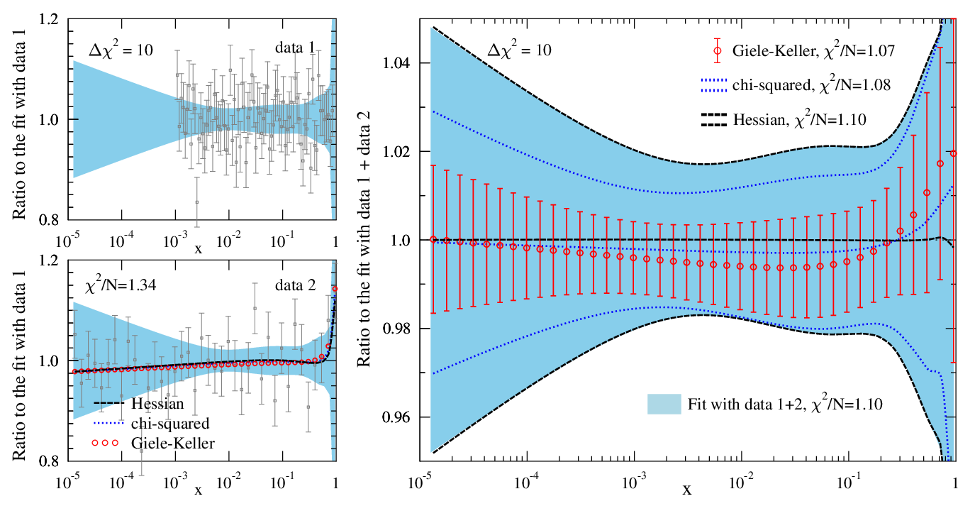
Many global fits of PDFs use $\Delta\chi^{2}$ clearly larger than unity. In our simple example here, a motivation for using $\Delta\chi^{2}>1$ could be to compensate for the restricted functional form at small values of $x$ where the data set 1 did not have constraints [28]. Thus, we repeat the exercise taking this time $\Delta\chi^{2}=10$. The results are shown in Figure 4. While the Hessian reweighting can still accurately reproduce the re-fit, neither of the Bayesian methods coincides with them. In the case of GK reweighting the reason for the failure is that the likelihood function $\mathcal{P}(\vec{y}|f)$ as such does not contain any information on $\Delta\chi^{2}$, although the distribution of replicas clearly depends on the value of $\Delta\chi^{2}$. As the spread among the replicas encoded by $\Delta\chi^{2}=1$ is narrower than that covered by $\Delta\chi^{2}=10$, the new data appear more constraining than they actually are. This can also be verified from the distribution of Bayesian weights shown in the right-hand panel of Figure 3. In comparison to the case with $\Delta\chi^{2}=1$ the replicas with lowest $\chi^{2}$ tend to get much higer weight.

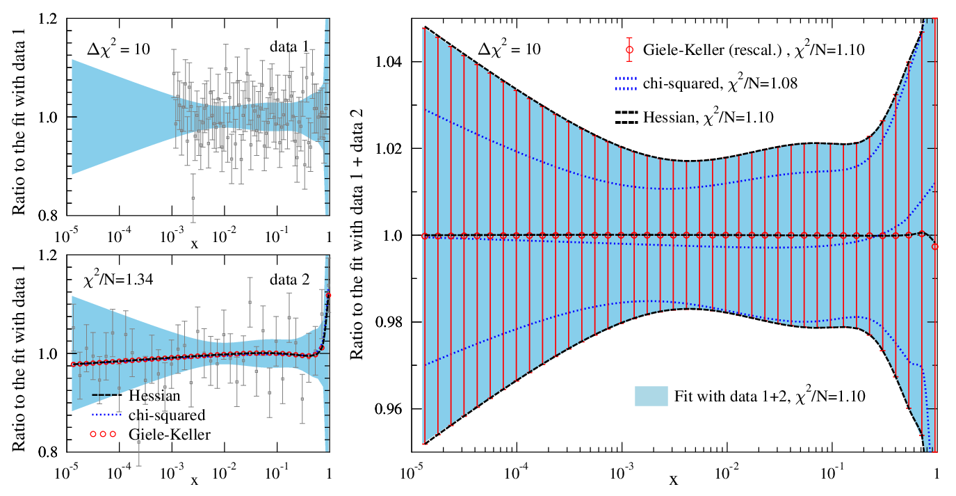
However, the agreement encountered with $\Delta\chi^{2}=1$ (Figure 2) hints that it should be possible to generalize the Bayesian method with GK weights also to the case with $\Delta\chi^{2}>1$. The key point is to note that we could divide, for example, Eq. (12) by $\Delta\chi^{2}$, and effectively use $\Delta\chi^{2}=1$ thereafter. This observation instructs us to rescale the values of $\chi^{2}_{k}$ in Eqs. (33) as

$$\chi^{2}_{k}\longrightarrow\frac{\chi^{2}_{k}}{\Delta\chi^{2}},$$

(42)

when computing the weight for each replica. The corresponding results are shown in Figure 5 which differs from Figure 4 only in using the above mentioned rescaling when computing the Bayesian GK weights. Evidently, the agreement between the Bayesian method with GK weights, the Hessian reweighting, and the re-fit, is restored. The spectrum of rescaled GK weights is shown in the right-hand panel of Figure 3 as well. The division of the individual $\chi^{2}$ values by $\Delta\chi^{2}$ makes the distribution of weights considerably flatter and it is actually a rather wide range of $\chi^{2}$ values that still give a non-negligible contribution. We note that mathematically we would end up with the same reweighting result by narrowing the Gaussian distribution of random numbers instead of rescaling the individual $\chi^{2}$ values. Indeed, replacing $R_{ik}\rightarrow R_{ik}/\sqrt{\Delta\chi^{2}}$ in Eq. (36) we would recover the same distribution of replicas that was obtained by using $\Delta\chi^{2}=1$. However, with $\Delta\chi^{2}=10$ and rescaled GK weights the effective number of replicas is about twice as large as that with $\Delta\chi^{2}=1$ ($N_{\rm eff,\Delta\chi^{2}=1}\approx 19200$, $N_{\rm eff,\Delta\chi^{2}=10}\approx 37500$). This makes the rescaling of $\chi^{2}$ values a better option that narrowing the Gaussian distribution, although both procedures lead to the same result.

Our simple example here indicates that the Bayesian reweighting with chi-squared weights does not, in general, correspond to a direct re-fit although here they lead to a good approximation.⁴⁴ 4 In a situation in which many replicas give $\chi_{k}^{2}/N_{\rm data}\ll 1$ the difference to the direct re-fit can become much larger. However, comparing Figures 2 and 5 we notice that for $\Delta\chi^{2}=1$ the results of chi-squared reweighting are a bit above the true result, but for $\Delta\chi^{2}=10$ somewhat below. Similarly, for $\Delta\chi^{2}=1$ the errorband is too wide, but for $\Delta\chi^{2}=10$ too narrow. It therefore looks possible that by “tuning” the $\Delta\chi^{2}$ appropriately the chi-squared reweighting could be made to coincide with the exact result. Since the rescaled GK weights appear to be the proper way to do the reweighting, the condition that the replicas that mostly contribute get the same weight in both cases is that the ratio

$$r\equiv\frac{\left(\chi^{2}\right)^{(N_{\rm data}-1)/2}\exp\left[-\chi^{2}/2\right]}{\exp\left[-\chi^{2}/(2\Delta\chi^{2})\right]}$$

(43)

is approximately constant. Requiring the derivative of this ratio to be zero, one finds

$$\Delta\chi^{2}_{\big|{\frac{dr}{d\chi^{2}}=0}}=\frac{\chi^{2}}{\chi^{2}-(N_{\rm data}-1)}.$$

(44)

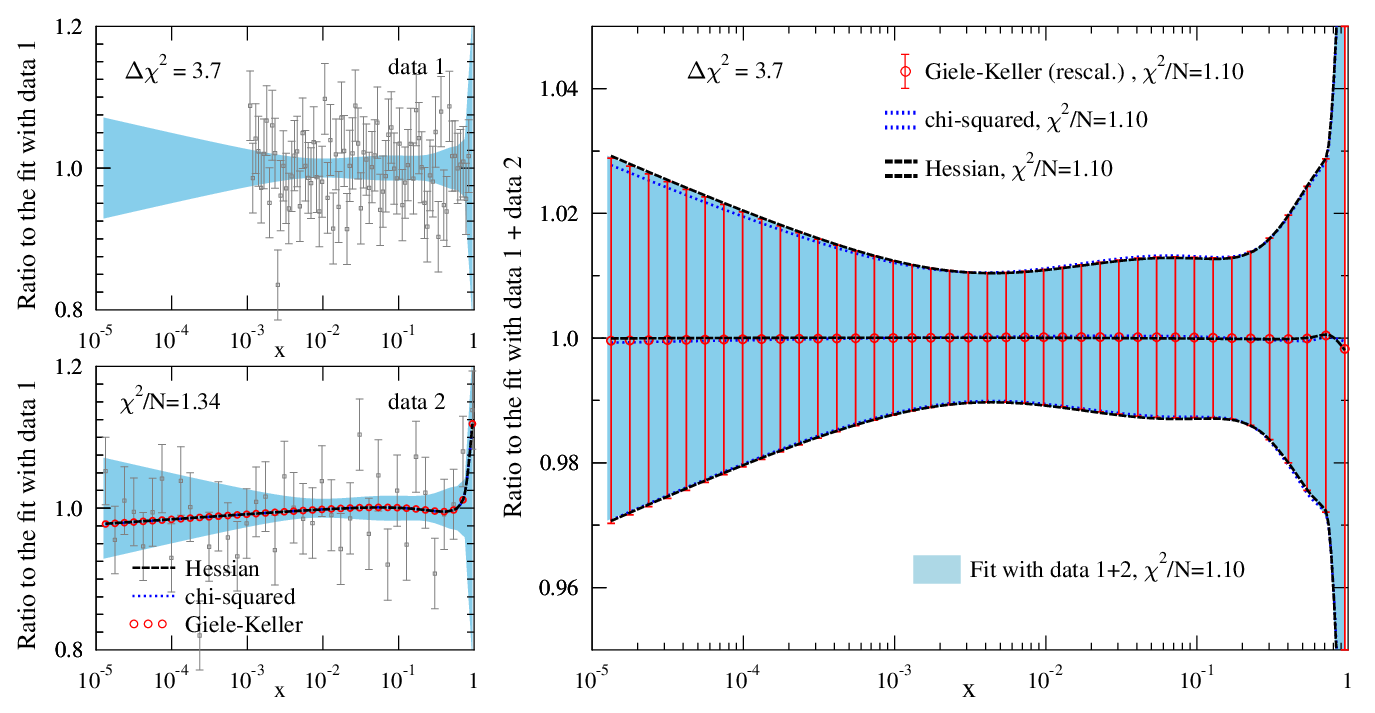
The individual replicas are always centered around the original fit and it thus makes sense to take the original value of $\chi^{2}$ as a guideline in evaluating the value of $\Delta\chi^{2}$ in the equation above. In the present example $\chi^{2}/N\approx 1.34$ before the re-fit which corresponds to $\Delta\chi^{2}\approx 3.7$. This particular value of $\Delta\chi^{2}$ brings the chi-squared method to an excellent agreement with the direct re-fit as can be seen from Figure 6. The corresponding distributions of the Bayesian weights are shown in Figure 7 and, indeed, with $\Delta\chi^{2}\approx 3.7$ the chi-squared and rescaled GK weights go practically hand in hand in the region of $\chi^{2}$ which mostly contributes to the final result. That is, if most of the replicas give $\chi^{2}/N>1$ and $\Delta\chi^{2}$ happens to be close to the value of Eq. (44) evaluated with the original central $\chi^{2}$, both Bayesian reweightings may give approximately the same result.

In our simple example here, what mainly limits the accuracy of the reweighting is the precision of the original quadratic expansion of Eq. (2). Indeed, the small mismatch between the results of reweighting and the real fit e.g. in Figure 5 can be largely attributed to this approximation not being perfect. Although the same function $g(x)$ was used in generating and fitting the pseudodata, we have checked that using a different fit function, e.g. a superposition of Chebysev polynomials, would not alter our conclusions.

The close similarity of the results obtained using the (linear) Hessian reweighting and Bayesian one with the rescaled GK weights indicates that the two are actually one and the same. In this short section we will give a formal proof of this equivalence. From Eq. (38) we see that the coordinates specifying the GK-reweighted PDFs in the eigenvector space are given by

$$w_{k}^{\rm GK}=\frac{1}{N_{\rm rep}}\sum_{\ell}^{N_{\rm rep}}\omega_{\ell}R_{k\ell}=\frac{1}{\mathcal{N}}\times\frac{1}{N_{\rm rep}}\sum_{\ell}^{N_{\rm rep}}e^{-\frac{\chi^{2}_{\ell}}{2\Delta\chi^{2}}}R_{k\ell},$$

(45)

where the denominator $\mathcal{N}$ is

$$\mathcal{N}\equiv\frac{1}{N_{\rm rep}}\sum_{\ell}^{N_{\rm rep}}e^{-\frac{\chi^{2}_{\ell}}{2\Delta\chi^{2}}},$$

(46)

and we have applied the rescaling $\chi^{2}_{k}\rightarrow{\chi^{2}_{k}}/{\Delta\chi^{2}}$ as in Eq. (42). Using the expression for $\chi^{2}$ in Eq. (34) and the linear approximation of Eq. (13) with $w_{k}=R_{k\ell}$, we find

	$\displaystyle w_{k}^{\rm GK}=\frac{1}{\mathcal{N}}\times\frac{1}{N_{\rm rep}}\sum_{\ell}^{N_{\rm rep}}\exp\bigg[$		$\displaystyle\hskip-5.69046pt-\frac{1}{2\Delta\chi^{2}}\sum_{n,m}^{N_{\rm eig}}R_{n\ell}\left(\sum_{i,j}D_{in}C^{-1}_{ij}D_{jm}\right)R_{m\ell}$		(47)
			$\displaystyle\hskip-5.69046pt-\frac{1}{\Delta\chi^{2}}\sum_{n}^{N_{\rm eig}}a_{n}R_{n\ell}-\frac{1}{2\Delta\chi^{2}}\,\chi^{2}[f_{S_{0}}]\bigg]R_{k\ell},$

where $\chi^{2}[f_{S_{0}}]$ is the value of $\chi^{2}$ computed with the central set $S_{0}$, and the coefficients $D_{ik}$ and $a_{k}$ were defined in Eqs. (14) and (18). In the limit of infinitely large $N_{\rm rep}$, the sum over the replicas above can be replaced by an integral

$$\frac{1}{N_{\rm rep}}\sum_{\ell=1}^{N_{\rm rep}}\xrightarrow{N_{\rm rep}\rightarrow\infty}\left(2\pi\right)^{-N_{\rm eig}/2}\int_{-\infty}^{+\infty}d\vec{\bf R}\exp\left[-\frac{1}{2}\vec{\bf R}^{2}\right],$$

(48)

where the additional exponential stems from the probability distribution for the random numbers $R_{m\ell}$ being Gaussian. Using this in Eq. (47) above, we have

	$\displaystyle w_{k}^{\rm GK}$	$\displaystyle=$	$\displaystyle\frac{1}{\mathcal{N}}\times\left(2\pi\right)^{-N_{\rm eig}/2}e^{-\frac{1}{2\Delta\chi^{2}}\,\chi^{2}[f_{S_{0}}]}\int_{-\infty}^{+\infty}d\vec{\bf R}e^{-\frac{1}{2\Delta\chi^{2}}\vec{\bf R}^{T}{\bf B}\vec{\bf R}-\frac{1}{\Delta\chi^{2}}\vec{\bf a}^{T}\vec{\bf R}}R_{k}$
		$\displaystyle=$	$\displaystyle-\frac{\Delta\chi^{2}}{\mathcal{N}}\times\left(2\pi\right)^{-N_{\rm eig}/2}e^{-\frac{1}{2\Delta\chi^{2}}\,\chi^{2}[f_{S_{0}}]}\frac{d}{da_{k}}\int_{-\infty}^{+\infty}d\vec{\bf R}e^{-\frac{1}{2\Delta\chi^{2}}\vec{\bf R}^{T}{\bf B}\vec{\bf R}-\frac{1}{\Delta\chi^{2}}\vec{\bf a}^{T}\vec{\bf R}}$
		$\displaystyle=$	$\displaystyle-\frac{1}{\mathcal{N}}\times\sqrt{\frac{(\Delta\chi^{2})^{N_{\rm eig}}}{\det{\bf B}}}e^{-\frac{1}{2\Delta\chi^{2}}\,\chi^{2}[f_{S_{0}}]+\frac{1}{2\Delta\chi^{2}}\vec{\bf a}^{T}{\bf B}^{-1}\vec{\bf a}}({\bf B}^{-1}\vec{\bf a})_{k},$

where the elements of the matrix ${\bf B}$ were given in Eq. (17). The corresponding expression for the denominator $\mathcal{N}$ is

$\displaystyle\mathcal{N}=\sqrt{\frac{(\Delta\chi^{2})^{N_{\rm eig}}}{\det{\bf B}}}e^{-\frac{1}{2\Delta\chi^{2}}\,\chi^{2}[f_{S_{0}}]+\frac{1}{2\Delta\chi^{2}}\vec{\bf a}^{T}{\bf B}^{-1}\vec{\bf a}}.$

(49)

Upon taking the ratio, the various prefactors cancel, and the coefficients $w_{k}^{\rm GK}$ reduce to

$$w_{k}^{\rm GK}=-({\bf B}^{-1}\vec{\bf a})_{k},$$

(50)

which coincides with the Eq. (16) specifying the coefficients for the linear Hessian reweighting. As shown in Ref. [23], the weights $w_{k}^{\rm chi-squared}$ in Eq. (35) emerge from $w_{k}^{\rm GK}$ by integrating over all possible data sets that give equal $\chi^{2}$. Being “contaminated” by such additional information readily explains their failure in the present context.

In this section, we apply the reweighting methods to the production of inclusive jets in proton+proton collisions at the LHC. In comparison to our example discussed earlier, a new source of non-linearity arises which could potentially decrease the accuracy of the linear reweighting. Namely, the quadratic PDF dependence of the proton+proton cross sections ($\hat{\sigma}$ denotes the coefficient functions and jet definitions in general)

$$\sigma^{\rm pp}[S]=f[S]\otimes\hat{\sigma}\otimes f[S],$$

(51)

may or may not be well approximated by

$\displaystyle\sigma^{\rm pp}[S_{0}+\frac{1}{2}\sum_{k}\left(S^{+}_{k}-S^{-}_{k}\right)w_{k}]\approx\sigma^{\rm pp}[S_{0}]+\frac{1}{2}\sum_{k}\left(\sigma^{\rm pp}[S^{+}_{k}]-\sigma^{\rm pp}[S^{-}_{k}]\right)w_{k},$

(52)

which is the approximation one effectively makes when using Eq. (13). In some other cases, such as deep-inelastic scattering (linear in PDFs), this would not be an issue whereas for the $W$-asymmetry, the non-linearities could be even more intricate. Here, we consider the recent CMS $\sqrt{s}=7\,{\rm TeV}$ jet measurements [30] ($N_{\rm data}=133$) for which a direct FASTNLO interface [31, 32, 33] is available to evaluate the cross sections at NLO accuracy. We use the CTEQ6.6 PDFs [34] whose error sets quantify the uncertainties within 90% confidence level the corresponding tolerance being $\Delta\chi^{2}_{\rm CTEQ6.6}(90\%)=100$.

The renormalization scale $\mu_{r}$ and factorization scale $\mu_{f}$ were fixed to the jet transverse momentum as $\mu_{r}=\mu_{f}=p_{T}/2$, and the strong coupling was set to $\alpha_{s}(M_{Z})=0.118$ at the Z boson pole.

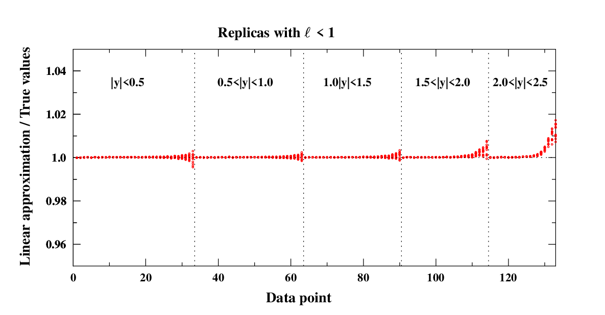
Let us first discuss the adequacy of the approximation in Eq. (52). To this end, we have prepared some random PDF replicas by Eq. (36) separating the cases $\ell=\sum_{i=1}^{N_{\rm eig}}R_{ik}^{2}<1$ and $\ell=\sum_{i=1}^{N_{\rm eig}}R_{ik}^{2}>1$. We compute the jet cross sections “exactly” (by constructing parametrizations corresponding to these PDF replicas and using them in FASTNLO computations) and, on the other hand, by the linear approximation of Eq. (52). Typical results from such an exercise are shown in Figure 8. First, if $\ell<1$, the linear approximation proves rather accurate, the deviations being normally much less than couple of percents. In the latter case, $\ell>1$, the linear approximation evidently breaks down. We conclude that if the reweighted PDFs end up sufficiently close to the original ones the linear approximation of Eq. (52), and thereby the linear Hessian reweighting, should be rather accurate. In the case of Bayesian reweighting, replicas with $\ell>1$ often occur, and, from the lower panel of Figure 8, we can consequently anticipate some differences whether the cross sections are evaluated using the replicas directly inside FASTNLO, or “on the fly” by the linear approximation of Eq. (52).

We account for the correlated systematic errors by constructing a covariance matrix. To be specific, we compute the elements of the covariance matrix $C$ by

$$C_{ij}=\delta_{ij}\left(\sigma_{i}^{\rm uncorr}\right)^{2}+\sum_{k}\beta_{i}^{k}\beta_{j}^{k},$$

(53)

where $\sigma_{i}^{\rm uncorr}$ is the uncorrelated error of data point $i$, and $\beta_{i}^{k}$ denotes the absolute shift of this data point corresponding to 1-sigma deviation of the systematic parameter $k$. In addition to the luminosity, unfolding and jet energy scale uncertainties, we also treat the quoted uncertainty in the multiplicative non-perturbative corrections (underlying event, hadronization) as a correlated systematic error. The uncorrelated errors $\sigma_{i}^{\rm uncorr}$ include the statistical and 1% uncorrelated systematic uncertainty added in quadrature. Calculating the $\chi^{2}$ using the covariance matrix $C$ is equivalent to (see e.g. [35, 36, 37]) minimizing

$$\chi^{2}=\sum_{i}\left[\frac{y_{i}^{\rm theory}-y_{i}^{\rm data}-\sum_{k}s_{k}\beta_{i}^{k}}{\sigma_{i}^{\rm uncorr}}\right]^{2}+\sum_{k}s_{k}^{2},$$

(54)

with respect to the systematic parameters $s_{k}$. This occurs with the parameter values

$$s_{k}^{\rm min}=\sum_{j}\left[\beta_{j}^{k}-\sum_{i,\ell,s}\beta_{i}^{k}C_{i\ell}^{-1}\beta_{\ell}^{s}\beta_{j}^{s}\right]\frac{y_{j}^{\rm theory}-y_{j}^{\rm data}}{(\sigma_{j}^{\rm uncorr})^{2}},$$

(55)

and $-\sum_{k}s^{\rm min}_{k}\beta_{i}^{k}$ is the net systematic shift for the data point $y_{i}^{\rm data}$. Figure 9 presents a comparison between the CMS data and the NLO predictions, including the 68% PDF error bands (obtained downscaling the original 90% errors by $1/1.645$ [11, 38]). The $\chi^{2}$ value for the central CTEQ6.6 set is $\chi^{2}/N_{\rm data}\approx 2.1$ accounting for the data correlations as discussed above. The calculation appears to overpredict the experimental cross section by some 5% which, however, gets still easily hidden under the systematic shifts as demonstrated in Figure 9.

It is a straightforward task to apply the reweighting methods on these jet data. For the needs of the Bayesian techniques we have generated $10^{4}$ PDF replicas using Eq. (36). As the data uncertainties correspond to one standard deviation, we have rescaled the random numbers in Eq. (36) by $R_{ik}\rightarrow R_{ik}/1.645$ which brings the PDF replicas to the 68% level as well. When computing the GK weights we divide the resulting values of $\chi^{2}$ by $\Delta\chi^{2}_{\rm CTEQ6.6}(68\%)=100/1.645^{2}\approx 37$, to appropriately modify the underlying likelihood. The chi-squared weights are always computed without rescaling the $\chi^{2}$ values. We stress that the rescaling of CTEQ6.6 replicas from 90% to 68% confidence level affects only the outcome of chi-squared reweighting as, by construction, the central result of GK reweighting would remain the same by simply using the 90% replicas and rescaling the $\chi^{2}$ values by $\Delta\chi^{2}_{\rm CTEQ6.6}(90\%)$. The Hessian reweighting has been performed directly with the original 90% error sets rescaling the uncertainties by $1/1.645$ only at the end. The resulting modifications in the gluon PDFs are presented in the upper panel of Figure 10 (as the jet production is predominantly sensitive to the gluons, we find it reasonable to present the results here only in terms of gluon PDFs). From this plot we find that, as expected, the Hessian technique and the Bayesian method with rescaled GK weights are in good agreement also here. The small mismatch at large $x$ originates mainly from Eq. (52) not being exact. As the reweighting penalty $P\approx 21$ is less than $\Delta\chi^{2}_{\rm CTEQ6.6}(68\%)$, we conclude that these data could have been added to the CTEQ6.6 fit without causing a significant disagreement with the original data. In this sense these data are compatible with the CTEQ6.6 PDFs despite the largish $\chi^{2}/N_{\rm data}\approx 1.75$ which could hint, however, that some tension between the Tevatron Run-1 jet data [39, 40] (used in CTEQ6.6 fit to constrain large-$x$ gluons) and these new LHC measurements exist.⁵⁵ 5 Indeed, the latest CTEQ fit [35] has abandoned the Tevatron Run-1 jet data as they do not completely agree with the Run-2 data. See Ref. [5] for a review and Ref. [41] for more discussions.

The line of red points in Figure 10 shows the spectrum of rescaled GK weights. For dividing the values of $\chi^{2}$ by the tolerance $\Delta\chi^{2}_{\rm CTEQ6.6}(68\%)\approx 37$, this distribution is rather flat and the final result is affected by replicas with a wide range of $\chi^{2}$ explaining also the rather large number of effective replicas, $N_{\rm eff}/N_{\rm rep}~\approx 0.72$. The chi-squared weights give rise to effects which are qualitatively alike but quantitatively much larger. The agreement with the new jet data is admittedly better, $\chi^{2}/N_{\rm data}\approx 1.15$ (the green points in Figure 10 indeed demonstrate that the chi-squared weights assign clearly larger weights to replicas with $\chi^{2}/N_{\rm data}<1.4$ than the rescaled GK weights), but at the cost of increasing the original $\chi^{2}$ by $P\approx 290$ which is way beyond the CTEQ6.6 tolerance (both 68% and 90%). The surviving number of replicas $N_{\rm eff}$ is also very low. That is, one could conclude that the jet data considered here were not in agreement with the CTEQ6.6 PDFs. However, as we have demonstrated in the previous sections, the result is misleading since the chi-squared weights do not appropriately account for the other data that were originally included in the global CTEQ6.6 fit. From Eq. (44) we can estimate the value of $\Delta\chi^{2}$ that would have brought the results of chi-squared reweighting close to the correct ones: using the original central value $\chi^{2}/N_{\rm data}\approx 2.1$ and $N_{\rm data}=133$ we obtain $\Delta\chi^{2}\approx 1.9$. This is much less than $\Delta\chi^{2}_{\rm CTEQ6.6}(68\%)=37$ and concretely explains why the chi-squared weights lead to a result which is so far from the correct one.

The new predictions for the cross-section are shown in Figure 11. The systematic shifts have been applied to the data and they depend significantly on which method of reweighting was used. The Hessian reweighting has caused a mild downward shift on the cross section which was to be expected given that the original central predictions somewhat overshoot the data (see Figure 9). In the case of Bayesian reweighting with chi-squared weights the induced changes with respect to the original CTEQ6.6 predictions are way too large.

References

- (1) J. C. Collins, D. E. Soper and G. F. Sterman, Adv. Ser. Direct. High Energy Phys. 5 (1988) 1 [hep-ph/0409313].
- (2) J. C. Collins, D. E. Soper and G. F. Sterman, Nucl. Phys. B 261 (1985) 104.
- (3) S. Forte and G. Watt, Ann. Rev. Nucl. Part. Sci. 63 (2013) 291 [arXiv:1301.6754 [hep-ph]].
- (4) H. -L. Lai, M. Guzzi, J. Huston, Z. Li, P. M. Nadolsky, J. Pumplin, C. -P. Yuan and , Phys. Rev. D 82 (2010) 074024 [arXiv:1007.2241 [hep-ph]].
- (5) A. D. Martin, W. J. Stirling, R. S. Thorne and G. Watt, Eur. Phys. J. C 63 (2009) 189 [arXiv:0901.0002 [hep-ph]].
- (6) R. D. Ball, V. Bertone, S. Carrazza, C. S. Deans, L. Del Debbio, S. Forte, A. Guffanti and N. P. Hartland et al., Nucl. Phys. B 867 (2013) 244 [arXiv:1207.1303 [hep-ph]].
- (7) W. T. Giele and S. Keller, Phys. Rev. D 58 (1998) 094023 [hep-ph/9803393].
- (8) R. D. Ball et al. [NNPDF Collaboration], Nucl. Phys. B 849 (2011) 112 [Erratum-ibid. B 854 (2012) 926] [Erratum-ibid. B 855 (2012) 927] [arXiv:1012.0836 [hep-ph]].
- (9) R. D. Ball, V. Bertone, F. Cerutti, L. Del Debbio, S. Forte, A. Guffanti, N. P. Hartland and J. I. Latorre et al., Nucl. Phys. B 855 (2012) 608 [arXiv:1108.1758 [hep-ph]].
- (10) S. Chatrchyan et al. [CMS Collaboration], Phys. Rev. D 90 (2014) 032004 [arXiv:1312.6283 [hep-ex]].
- (11) R. Gauld, JHEP 1402 (2014) 126 [arXiv:1311.1810 [hep-ph]].
- (12) M. Czakon, M. L. Mangano, A. Mitov and J. Rojo, JHEP 1307 (2013) 167 [arXiv:1303.7215 [hep-ph]].
- (13) L. Carminati, G. Costa, D. D’Enterria, I. Koletsou, G. Marchiori, J. Rojo, M. Stockton and F. Tartarelli, EPL 101 (2013) 61002 [Europhys. Lett. 101 (2013) 61002] [arXiv:1212.5511].
- (14) M. Beneke, P. Falgari, S. Klein, J. Piclum, C. Schwinn, M. Ubiali and F. Yan, JHEP 1207 (2012) 194 [arXiv:1206.2454 [hep-ph]].
- (15) D. d’Enterria and J. Rojo, Nucl. Phys. B 860 (2012) 311 [arXiv:1202.1762 [hep-ph]].
- (16) R. D. Ball et al. [NNPDF Collaboration], Nucl. Phys. B 877 (2013) 2, 290 [arXiv:1308.0598 [hep-ph]].
- (17) J. Pumplin, D. Stump, R. Brock, D. Casey, J. Huston, J. Kalk, H. L. Lai, W. K. Tung, Phys. Rev. D 65 (2001) 014013 [hep-ph/0101032].
- (18) G. Watt, R. S. Thorne, JHEP 1208 (2012) 052 [arXiv:1205.4024 [hep-ph]].
- (19) N. Sato, arXiv:1309.7995 [hep-ph].
- (20) N. Armesto, J. Rojo, C. A. Salgado and P. Zurita, JHEP 1311 (2013) 015 [arXiv:1309.5371 [hep-ph]].
- (21) B. J. A. Watt, P. Motylinski and R. S. Thorne, Eur. Phys. J. C 74 (2014) 2934 [arXiv:1311.5703 [hep-ph]].
- (22) H. Paukkunen and C. A. Salgado, Phys. Rev. Lett. 110 (2013) 212301 [arXiv:1302.2001 [hep-ph]].
- (23) N. Sato, J. F. Owens and H. Prosper, Phys. Rev. D 89 (2014) 114020 [arXiv:1310.1089 [hep-ph]].
- (24) A. M. Cooper-Sarkar [ZEUS and H1 Collaborations], PoS EPS -HEP2011 (2011) 320 [arXiv:1112.2107 [hep-ph]].
- (25) S. Alekhin, J. Blumlein and S. Moch, Phys. Rev. D 86 (2012) 054009 [arXiv:1202.2281 [hep-ph]].
- (26) J. F. Owens, A. Accardi and W. Melnitchouk, Phys. Rev. D 87 (2013) 094012 [arXiv:1212.1702 [hep-ph]].
- (27) J. Pumplin, D. R. Stump, J. Huston, H. L. Lai, P. M. Nadolsky and W. K. Tung, JHEP 0207 (2002) 012 [hep-ph/0201195].
- (28) J. Pumplin, Phys. Rev. D 82 (2010) 114020 [arXiv:0909.5176 [hep-ph]].
- (29) A. Glazov, S. Moch and V. Radescu, Phys. Lett. B 695 (2011) 238 [arXiv:1009.6170 [hep-ph]].
- (30) S. Chatrchyan et al. [CMS Collaboration], Phys. Rev. D 87 (2013) 112002 [arXiv:1212.6660 [hep-ex]].
- (31) T. Kluge, K. Rabbertz and M. Wobisch, hep-ph/0609285.
- (32) D. Britzger et al. [fastNLO Collaboration], arXiv:1208.3641 [hep-ph].
- (33) M. Wobisch et al. [fastNLO Collaboration], arXiv:1109.1310 [hep-ph].
- (34) P. M. Nadolsky, H. -L. Lai, Q. -H. Cao, J. Huston, J. Pumplin, D. Stump, W. -K. Tung and C. -P. Yuan, Phys. Rev. D 78 (2008) 013004 [arXiv:0802.0007 [hep-ph]].
- (35) J. Gao, M. Guzzi, J. Huston, H. -L. Lai, Z. Li, P. Nadolsky, J. Pumplin and D. Stump et al., arXiv:1302.6246 [hep-ph].
- (36) D. Stump, J. Pumplin, R. Brock, D. Casey, J. Huston, J. Kalk, H. L. Lai and W. K. Tung, Phys. Rev. D 65 (2001) 014012 [hep-ph/0101051].
- (37) S. Albino, B. A. Kniehl and G. Kramer, Nucl. Phys. B 803 (2008) 42 [arXiv:0803.2768 [hep-ph]].
- (38) S. Dulat, T. J. Hou, J. Gao, J. Huston, P. Nadolsky, J. Pumplin, C. Schmidt and D. Stump et al., Phys. Rev. D 89 (2014) 113002 [arXiv:1310.7601 [hep-ph]].
- (39) T. Affolder et al. [CDF Collaboration], Phys. Rev. D 64 (2001) 032001 [Erratum-ibid. D 65 (2002) 039903] [hep-ph/0102074].
- (40) B. Abbott et al. [D0 Collaboration], Phys. Rev. D 64 (2001) 032003 [hep-ex/0012046].
- (41) J. Pumplin, J. Huston, H. L. Lai, P. M. Nadolsky, W. -K. Tung and C. -P. Yuan, Phys. Rev. D 80 (2009) 014019 [arXiv:0904.2424 [hep-ph]].
- (42) G. Aad et al. [ATLAS Collaboration], Phys. Rev. D 86 (2012) 014022 [arXiv:1112.6297 [hep-ex]].