Error analysis of the transport properties of Metropolized schemesThanks: Funding from NEEDS “Milieux poreux” is gratefully acknowledged. We also benefited from the scientific environment of the Laboratoire International Associé between the Centre National de la Recherche Scientifique and the University of Illinois at Urbana-Champaign.Thanks: We thank Marie Jardat and Vincent Dahirel for fruitful discussions on the practical aspects of the numerical methods we study here.

Consider $N$ particles with positions $q=(q_{1},\dots,q_{N})$ in a cubic box of size $L>0$: $q\in\mathcal{M}=(L\mathbb{T})^{dN}$, $\mathbb{T}=\mathbb{R}/\mathbb{Z}$ being the standard one-dimensional torus and $d$ being the physical dimension (usually $d=3$). The positions of the particles evolve according to the following dynamics:

(1)

$$dq_{t}=-\beta\nabla V(q_{t})\,dt+\sqrt{2}\,dW_{t},$$

where $\beta=1/(k_{\rm B}T)$ is the inverse temperature ($k_{\rm B}$ being Boltzmann’s constant and $T$ being the temperature) and $W_{t}$ is a standard $dN$-dimensional Brownian motion. The function $V:\mathcal{M}\to\mathbb{R}$ is the potential energy, assumed to be smooth for the mathematical analysis. However, the numerical results presented in Section 3.2 correspond to a potential energy function with singularities.

Standard results (see for instance the references in [13, Section 2.2]) show that (1) admits the Boltzmann-Gibbs measure

(2)

$$\mu(dq)=Z^{-1}\,\mathrm{e}^{-\beta V(q)}\,dq,\qquad Z=\int_{\mathcal{M}}\mathrm{e}^{-\beta V},$$

as its unique invariant probability measure (note that $Z$ is finite since the position space $\mathcal{M}$ is compact and $V$ is smooth hence bounded). In fact, (1) is ergodic with respect to this measure, where ergodicity is understood both as (i) the long-time (almost-sure) convergence of averages along trajectories

$$\lim_{t\to+\infty}\frac{1}{t}\int_{0}^{t}f(q_{s})\,ds=\int_{\mathcal{M}}f(q)\,\mu(dq)\qquad\mathrm{a.s.}$$

for any initial condition $q_{0}\in\mathcal{M}$ and all observables $f\in L^{1}(\mu)$; or as (ii) the convergence of the law $\psi(t,q)\,dq$ of the process (1), happening here at an exponential rate, for instance in total variation: Denoting with some abuse of notation the measure $\psi(t,q)\,dq$ by $\psi(t)$, there exist $C,\lambda>0$ such that

$$\|\psi(t)-\mu\|_{\rm TV}\leqslant C\,\mathrm{e}^{-\lambda t},$$

where the total variation distance between two measures $\nu_{1},\nu_{2}$ is defined as

$$\|\nu_{1}-\nu_{2}\|_{\rm TV}=2\sup_{S\in\mathscr{B}(\mathcal{M})}\left|\nu_{1}(S)-\nu_{2}(S)\right|=\sup_{|\varphi|\leqslant 1}\left|\int_{\mathcal{M}}\varphi\,d\nu_{1}-\int_{\mathcal{M}}\varphi\,d\nu_{2}\right|,$$

the suprema being taken over all measurable sets of $\mathcal{M}$ for the first one, and over all bounded, measurable functions for the second one.

For further purposes, we introduce the generator of (1), namely the operator

(3)

$$\mathcal{L}=-\beta\nabla V\cdot\nabla+\Delta.$$

This operator (defined with domain $D(\mathcal{L})=H^{2}(\mu)$) is self-adjoint on the Hilbert space $L^{2}(\mu)$ endowed with the scalar product

$$\left\langle\varphi,\psi\right\rangle_{L^{2}(\mu)}=\int_{\mathcal{M}}\varphi\,\psi\,d\mu.$$

The operator $-\mathcal{L}$ moreover has a positive spectral gap (see for instance [13, Section 2] and references therein). Indeed, a simple computation shows that

(4)

$$-\left\langle\mathcal{L}\varphi,\varphi\right\rangle_{L^{2}(\mu)}=\frac{1}{\beta}\|\nabla\varphi\|^{2}_{L^{2}(\mu)}.$$

The Poincaré inequality $\|\varphi\|_{L^{2}(\mu)}\leqslant C_{\mathcal{M},V}\|\nabla\varphi\|_{L^{2}(\mu)}$, valid for any function belonging to

$$\widetilde{L}^{2}(\mu)=\left\{\varphi\in L^{2}(\mu)\,\left|\int_{\mathcal{M}}\varphi\,d\mu=0\right.\right\},$$

allows to conclude that

(5)

$$\forall\varphi\in\widetilde{L}^{2}(\mu),\qquad-\left\langle\mathcal{L}\varphi,\varphi\right\rangle_{L^{2}(\mu)}\geqslant\frac{1}{\beta C_{\mathcal{M},V}}\|\varphi\|_{L^{2}(\mu)}^{2},$$

which shows that the spectral gap is larger or equal to $C_{\mathcal{M},V}^{-1}$. In particular, the resolvent $\mathcal{L}^{-1}$ is a well-defined operator on $\widetilde{L}^{2}(\mu)$, and the following estimate holds:

(6)

$$\left\|\mathcal{L}^{-1}\right\|_{\mathcal{B}\left(\widetilde{L}^{2}(\mu)\right)}\leqslant\beta C_{\mathcal{M},V}.$$

Here and in the sequel, for a given Banach space $X$, we denote by $\mathcal{B}(X)$ the Banach space of bounded operators on $X$, endowed with the norm

$$\|A\|_{\mathcal{B}(X)}=\sup_{x\in X\backslash\{0\}}\frac{\|Ax\|_{X}}{\|x\|_{X}}.$$

The positions $q_{t}$ are restricted to the periodic domain $\mathcal{M}$ and are therefore uniformly bounded in time. To obtain a diffusive behavior from the evolution of $q_{t}$, we consider the following additive functional defined on the whole space $\mathbb{R}^{d}$: starting from $Q_{0}=q_{0}$,

(7)

$$Q_{t}=Q_{0}-\beta\int_{0}^{t}\nabla V(q_{s})\,ds+\sqrt{2}\,W_{t}.$$

The difference with $q_{t}$ is that $Q_{t}$ is not reprojected in $\mathcal{M}$ by the periodization procedure (By this, we mean that we do not choose among all the images of $Q_{t}$ by translations of the lattice $L\mathbb{Z}^{d}$ the one for which all components are in the interval $[0,L)$). The diffusion tensor is then given by the following limit (provided it exists):

(8)

$$\mathscr{D}=\lim_{t\to+\infty}\mathbb{E}\left(\frac{Q_{t}-Q_{0}}{\sqrt{t}}\otimes\frac{Q_{t}-Q_{0}}{\sqrt{t}}\right),$$

where the expectation is over all realizations of the continuous dynamics (1), starting from initial conditions distributed according to the Boltzmann-Gibbs measure (2). The following result shows that the diffusion tensor (8) is well defined, and naturally arises in a diffusive time-rescaling of the dynamics (1).

The proof of this statement is standard, and follows from arguments presented in [1, Chapter 3] for instance. We nonetheless provide a short proof in Section 5.1 since the proofs of the discrete counterparts of Theorem 1 rely on an appropriate extension of the argument used in the continuous case (see Section 5.5).

A straightforward consequence of Theorem 1 is that the self-diffusion constant $\mathcal{D}$, defined as the average mean-square displacement of the individual particles, is well defined and has two equivalent expressions:

(10)		$\displaystyle\mathcal{D}=\frac{1}{2dN}\mathrm{Tr}(\mathscr{D})$	$\displaystyle=\lim_{t\to+\infty}\mathbb{E}\left(\frac{1}{2dNt}\sum_{i=1}^{N}(Q_{i,t}-Q_{i,0})^{2}\right)$
(11)			$\displaystyle=1-\frac{\beta^{2}}{dN}\int_{0}^{+\infty}\mathbb{E}\Big[\nabla V(q_{t})^{T}\nabla V(q_{0})\Big]dt.$

The expression (10) is called the Einstein formula. The second expression (11) involves an integrated autocorrelation function. In accordance with the standard physics and chemistry nomenclature, we call (11) the Green-Kubo formula for the self-diffusion in the sequel.

In order to compute approximations of formulas such as (10) or (11), the first task is to numerically integrate realizations of the continuous dynamics (1). The most straightforward way would be to resort to a Euler-Maruyama scheme: given a time-step $\Delta t>0$ and denoting by $q^{n}$ an approximation of $q_{n\Delta t}$, this scheme reads

(12)

$$q^{n+1}=q^{n}-\beta{\Delta t}\,\nabla V(q^{n})+\sqrt{2{\Delta t}}\,G^{n},$$

where $(G^{n})_{n\geqslant 0}$ is a sequence of independent and identically distributed (i.i.d.) $dN$-dimensional standard Gaussian random variables. However, this simple scheme has been shown to fail to be ergodic when the dynamics is considered on unbounded spaces and the potential energy function is not globally Lipschitz [14]. In simulations of Brownian dynamics for ionic solutions, potential energy functions with Coulomb-type singularities are used and it has been observed that the energy blows up along trajectories of (12) (see Section 3.2).

A way to stabilize the Euler-Maruyama scheme is to consider the configuration (12) as a proposal move in a Metropolis-Hastings algorithm [15, 8]. This is precisely the Smart MC algorithm proposed in [19] which was later called Metropolis adjusted Langevin algorithm in the computational statistics literature [18]. More precisely, starting from a configuration $q^{n}\in\mathcal{M}$ (in fact seen as an element of $\mathbb{R}^{dN}$), a new configuration $\widetilde{q}^{n+1}\in\mathbb{R}^{dN}$ is proposed according to (12), and then accepted with probability

$$R_{\Delta t}\left(q^{n},\widetilde{q}^{n+1}\right)=\min\left(\frac{\mathrm{e}^{-\beta V(\widetilde{q}^{n+1})}T_{\Delta t}(\widetilde{q}^{n+1},q^{n})}{\mathrm{e}^{-\beta V(q^{n})}T_{\Delta t}(q^{n},\widetilde{q}^{n+1})},1\right),$$

where

$$T_{\Delta t}(q,q^{\prime})=\left(\frac{1}{4\pi{\Delta t}}\right)^{dN/2}\exp\left(-\frac{|q^{\prime}-q+\beta{\Delta t}\nabla V(q)|^{2}}{4{\Delta t}}\right)$$

is the probability transition of the Markov chain (12). When the proposition is accepted, we project $\widetilde{q}^{n+1}$ into the periodic simulation cell $\mathcal{M}$. If the proposal is rejected, the previous configuration is counted twice: $q^{n+1}=q^{n}$ (It is very important to count rejected configuration as many times as needed to ensure that the Boltzmann-Gibbs measure $\mu$ is invariant). In conclusion,

(13)

$$q^{n+1}=q^{n}+\mathbf{1}_{U^{n}\leqslant R_{\Delta t}\left(q^{n},\widetilde{q}^{n+1}\right)}\left(-\beta{\Delta t}\,\nabla V(q^{n})+\sqrt{2{\Delta t}}\,G^{n}\right),$$

where $U^{n}$ are i.i.d. uniform random variables in $[0,1]$, and $\mathbf{1}_{U^{n}\leqslant\alpha}$ is an indicator function whose value is 1 when $U^{n}\leqslant\alpha$ and 0 otherwise. The average rejection rate is

(14)

$$1-R_{\Delta t}\left(q^{n},\widetilde{q}^{n+1}\right)=1-\mathbb{E}_{U}\Big(\mathbf{1}_{U\leqslant R_{\Delta t}\left(q^{n},\widetilde{q}^{n+1}\right)}\Big).$$

In the formula (13), $q^{n+1}$ is considered as an element of the periodic box $\mathcal{M}$, while the proposed configuration $\widetilde{q}^{n+1}$ is not reprojected into the simulation cell $\mathcal{M}$ and is therefore considered as an element of $\mathbb{R}^{dN}$ (see the remark after (7)).

In order to avoid confusion, we call the scheme (13) “Metropolized Euler-Maruyama” in the sequel, and denote by $P_{\Delta t}$ its evolution operator:

$$P_{\Delta t}f(q)=\mathbb{E}\Big(f\left(q^{n+1}\right)\,\Big|\,q^{n}=q\Big).$$

By construction, the measure (2) is an invariant probability measure for this scheme, which is a reversible Markov chain. We refer to [4] for a study of the ergodic properties of the dynamics (in the more complicated case of dynamics on the full configuration space $\mathbb{R}^{dN}$, subjected to a confining potential).

Of course, the fact that some configurations are rejected destroys the trajectorial accuracy of the dynamics, see [5] for precise statements. The resulting strong errors and, as a consequence, errors on finite time correlation functions have been quantified in [5, 6], with prefactors which unfortunately depend on time. The estimates provided by these works therefore do not provide error estimates on diffusion coefficients, obtained either as infinite time integrals of correlation functions as in the Green-Kubo formula (11) or as the infinite time average mean square displacement as in Einstein’s formula (10).

The next section quantifies the errors in the approximation of (10) and (11) when the Metropolized Euler-Maruyama scheme is used. Although the formulas (10) and (11) are equivalent for continuous dynamics, they lead to different numerical methods. Let us already emphasize that the errors on the diffusion coefficients are in fact determined by the expansion of the evolution operator $P_{\Delta t}$. This expansion is the same as the one used to establish weak error estimates. From a technical viewpoint, the techniques used in the proofs of our main results are therefore quite different from the techniques of [5, 6], which are based on strong error estimates obtained with Gronwall’s lemma.

We first give error estimates on (11) by appropriately adapting the results from [12]. The result is stated for two smooth observables $\psi,\varphi$ with average 0 with respect to $\mu$. Define to this end

$$\widetilde{C}^{\infty}(\mathcal{M})=\left\{\psi\in C^{\infty}(\mathcal{M})\,\left|\int_{\mathcal{M}}\psi\,d\mu=0\right.\right\}\subset\widetilde{L}^{\infty}(\mathcal{M}).$$

Error estimates for (11) are obtained by setting $\psi=\varphi=\partial_{q_{i,\alpha}}V$, with $1\leqslant i\leqslant N$ and $1\leqslant\alpha\leqslant d$. Note indeed that a simple integration by parts shows that $\partial_{q_{i,\alpha}}V$ has average 0 with respect to $\mu$, so $\partial_{q_{i,\alpha}}V\in\widetilde{C}^{\infty}(\mathcal{M})$.

As a corollary, we obtain first order error bounds on the computation of the self-diffusion through (11):

(20)

$$\mathcal{D}=\mathcal{D}^{\rm GK}_{\Delta t}+{\Delta t}\,\widetilde{\mathcal{D}}^{{\rm GK},1}+{\Delta t}^{3/2}\,\widetilde{\mathcal{D}}^{\rm GK}_{\Delta t},$$

where $\widetilde{\mathcal{D}}^{\rm GK}_{\Delta t}$ is uniformly bounded for ${\Delta t}$ sufficiently small, and where the numerically computed self-diffusion reads

(21)

$$\mathcal{D}^{\rm GK}_{\Delta t}=\mathrm{Id}-\frac{\beta^{2}}{dN}{\Delta t}\sum_{n=0}^{+\infty}\mathbb{E}_{\Delta t}\left[\nabla V(q^{n})^{T}\nabla V(q^{0})\right].$$

The expression of the correction term is obtained by replacing the modified observable by its expression:

$$\widetilde{\mathcal{D}}^{{\rm GK},1}_{\Delta t}=-\frac{\beta^{2}}{dN}{\Delta t}\sum_{n=0}^{+\infty}\mathbb{E}_{\Delta t}\left[F(q^{n})^{T}\nabla V(q^{0})\right],\qquad F=A\mathcal{L}^{-1}\nabla V.$$

The appearance of subleading fractional correction term in (20) (here, of order ${\Delta t}^{3/2}$) is typical of Metropolis algorithms, and is usually not encountered for standard, un-Metropolized discretizations of SDEs (compare with the results of [12]).

In this section, we investigate the discretization error made when using the Metropolized Euler-Maruyama scheme to approximate the self-diffusion using (10). In accordance with the definition (7), we introduce a discrete additive functional allowing to keep track of the diffuse behavior of the Markov chain: Starting from $Q^{0}=q^{0}$,

$$Q^{n}=\sum_{k=0}^{n-1}\delta_{\Delta t}\left(q^{k},G^{k},U^{k}\right),$$

with

(22)

$$\delta_{\Delta t}\left(q^{k},G^{k},U^{k}\right)=\mathbf{1}_{U^{k}\leqslant R_{\Delta t}\left(q^{k},q^{k}-\beta{\Delta t}\,\nabla V(q^{k})+\sqrt{2{\Delta t}}\,G^{k}\right)}\left(-\beta{\Delta t}\,\nabla V(q^{k})+\sqrt{2{\Delta t}}\,G^{k}\right).$$

While the Markov chain $(q^{n})_{n\geqslant 0}$ defined by (13) remains in $\mathcal{M}$, the additive functional $(Q^{n})_{n\geqslant 0}$ has values in $\mathbb{R}^{dN}$. The diffusion tensor actually computed by the numerical scheme is

(23)

$$\mathscr{D}^{\rm Einstein}_{\Delta t}=\lim_{n\to+\infty}\mathbb{E}_{\Delta t}\left[\frac{Q^{n}-Q^{0}}{\sqrt{n{\Delta t}}}\otimes\frac{Q^{n}-Q^{0}}{\sqrt{n{\Delta t}}}\right],$$

where, as in Theorem 2, the expectation on the right hand side is with respect to initial conditions $Q^{0}=q^{0}\sim\mu$ and for all realizations of the Metropolized Euler-Maruyama scheme.

The proof of this result can be read in Section 5.5. In fact, a slight extension of our technique of proof would allow to show that the diffusively rescaled process generated by the Metropolized Euler-Maruyama scheme, namely $\varepsilon Q^{\lfloor t/({\Delta t}\,\varepsilon^{2})\rfloor}$ (where $\lfloor x\rfloor$ denote the unique integer such that $\lfloor x\rfloor\leqslant x<\lfloor x\rfloor+1$), weakly converges on finite time intervals to a Brownian motion with covariance matrix $\mathscr{D}_{\Delta t}$.

An immediate corollary of Theorem 3 is the following a priori error estimate on the self-diffusion:

(24)

$$\mathcal{D}=\mathcal{D}^{\rm Einstein}_{\Delta t}+{\Delta t}\,\widetilde{\mathcal{D}}^{\rm Einstein}_{\Delta t},\qquad\mathcal{D}^{\rm Einstein}_{\Delta t}=\frac{1}{2dN}\mathrm{Tr}\left(\mathscr{D}^{\rm Einstein}_{\Delta t}\right),$$

where $\widetilde{\mathcal{D}}^{\rm Einstein}_{\Delta t}$ is uniformly bounded for ${\Delta t}$ sufficiently small. Some more work would allow to prove that the subleading correction term is of order ${\Delta t}^{3/2}$, as in the Green-Kubo case (see Remark 4).

We start by considering a simple one-dimensional example ($N=d=1$): a single particle in the unit torus $\mathcal{M}=\mathbb{T}$, with the periodic potential $V(q)=\cos(2\pi q)$, at $\beta=1$. Computations are performed by approximating expectations by realizations over $M$ replicas evolving independently, denoted by $q^{m,n}$ with $1\leqslant m\leqslant M$ and where $n$ still is the step index. Initial conditions are prepared incrementally over the replicas. More precisely, starting from $q^{1,0}=0$, we obtain the initial condition $q^{m+1,0}$ for the replica number $m+1$ by evolving the initial condition $q^{m,0}$ over 10 steps of the Metropolized Euler-Maruyama scheme with step size ${\Delta t}_{\rm thm}=0.01$. We have checked that the equilibrium distribution is very well reproduced by the empirical measure produced by $\{q^{m,0}\}_{1\leqslant m\leqslant M}$ provided $M$ is reasonably large (say, $M\geqslant 10^{3}$).

The self-diffusion coefficient $\mathcal{D}_{\Delta t}^{\rm Einstein}$ for the Einstein approach is approximated by fitting the unnormalized self-diffusion

(25)

$$D^{M}_{n}=\frac{1}{M}\sum_{m=1}^{M}\left(Q^{m,n}-Q^{m,0}\right)^{2}$$

by a linear function $\mathcal{D}^{{\rm Einstein},M}_{\Delta t}\,n{\Delta t}$, the slope being the estimation of the self-diffusion for the time step under consideration. This is indeed confirmed by Figure 1 (Left), which presents the evolution of $D_{n}^{M}$ as a function of the physical time $n{\Delta t}$. The results produced in Figures 1 and 3 have been obtained with $M=10^{7}$ replicas and $n_{\rm Einstein}=3\times 10^{5}$ steps. Let us also note that, in accordance with (17), the rejection rate scales as ${\Delta t}^{3/2}$.

A numerical approximation of (21) requires both a discretization using finitely many replicas, but also a truncation of the integration in time with an upper bound $\tau$. We consider the following numerical estimation of the self-diffusion coefficient obtained with the Green-Kubo formula:

(26)

$$\mathcal{D}^{{\rm GK},M,\tau}_{\Delta t}=1-\frac{\beta^{2}{\Delta t}}{M}\sum_{m=1}^{M}\sum_{n=0}^{\lfloor\tau/{\Delta t}\rfloor}V^{\prime}(q^{m,n})V^{\prime}(q^{m,0}).$$

The correlation functions shown in Figure 2 suggest that the autocorrelation of $V^{\prime}$ is exponentially decreasing. It can be considered as negligible for times larger than 0.2. The numerical results reported in Figure 2 and 3 have been obtained with $M=2\times 10^{8}$ replicas and a time cut-off $\tau=0.3$.

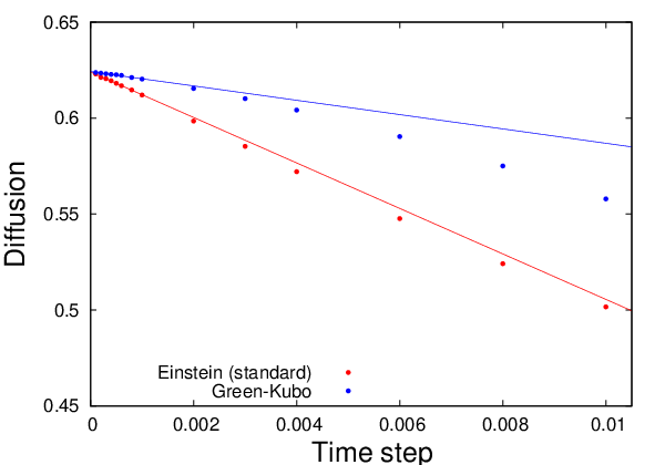
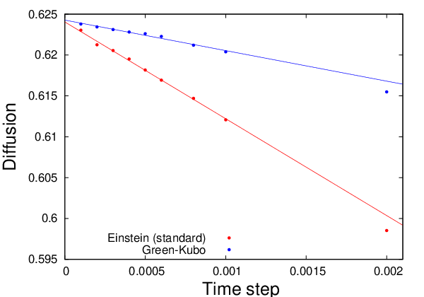
The results presented in Figure 3 indeed confirm that, for small time steps ${\Delta t}$, the error in the self-diffusion is of order ${\Delta t}$ for both methods. For larger time steps, nonlinearities appear. Note also that the errors on the coefficients computed with the Green-Kubo formula are smaller in this simple case. In any case, in accordance with the statements of Theorem 1, the self-diffusion is between 0 and 1 when ${\Delta t}\to 0$.

We consider in this section a more physically realistic system: a large, fixed ion interacting with smaller particles, typically smaller ions. The $N$ smaller particles evolve in a three-dimensional cubic simulation box of length $L$ with periodic boundary conditions. The smaller particles have the same mass $m$, and their positions are denoted by $q_{i}\in(L\mathbb{T})^{3}$. The potential energy functions are inspired by standard choices in the modeling of ionic solutions [10]. The interaction between small particles is governed by an appropriately truncated Lennard-Jones potential:

(27)

$$v(r)=4\varepsilon\left(\left(\frac{\sigma}{r}\right)^{12}-\left(\frac{\sigma}{r}\right)^{6}\right)-\varepsilon_{\mathrm{shift}}-f_{\mathrm{spline}}(r-r_{\rm cut}),\qquad\mathrm{when}\ r\leqslant r_{\rm cut},$$

and $v(r)=0$ for $r\geqslant r_{\rm cut}$. The parameter $\varepsilon>0$ is some reference energy, while $\sigma>0$ is some reference distance. The parameters $\varepsilon_{\mathrm{shift}}$ and $f_{\mathrm{spline}}$ ensure that $v$ is a $C^{1}$ function. When $r_{\rm cut}\to+\infty$, the minimal energy of $v$ converges to $-\varepsilon$, a value obtained at a distance $r_{\rm min}=2^{1/6}\sigma$.

We additionally consider a large ion, modeled as a fixed particle at position $q_{\rm ion}$ (the center of the simulation box), whose interaction with the solvent particles is described by an attractive Yukawa potential (screened Coulomb interaction) plus some repulsive potential preventing the small particles from coming too close to the ion. More precisely, for a solvent particle at position $q$, the interaction reads $v_{\rm ion}(|q-q_{\rm ion}|)$, with

(28)

$$v_{\rm ion}(r)=E_{\mathrm{min}}\left(1-\frac{1+\kappa\sigma}{24}\right)^{-1}\left(\frac{1+\kappa\sigma}{24}\left(\frac{\sigma}{r}\right)^{24}-\frac{\sigma}{r}\mathrm{e}^{-\kappa(r-\sigma)}\right)-\varepsilon_{\mathrm{shift}}^{\rm ion}-f_{\mathrm{spline}}^{\rm ion}(r-r_{\mathrm{cut}}^{\rm ion}),\qquad r\leqslant r_{\rm cut}^{\rm ion},$$

and $v_{\rm ion}(r)=0$ for $r\geqslant r_{\rm cut}^{\rm ion}$. The parameters $\varepsilon_{\mathrm{shift}}^{\rm ion}$ and $f_{\mathrm{spline}}^{\rm ion}$ ensure as above that $v_{\rm ion}$ is $C^{1}$. The energy $-E_{\mathrm{min}}\leqslant 0$ is the minimal value of the potential, obtained when $r=\sigma$ (in the limit when $r_{\rm cut}^{\rm ion}\to+\infty$ and $f_{\rm shift}^{\rm ion}=0$) while $\kappa$ is some inverse length. The total potential energy of the $N$ small particles finally reads

$$V(q_{1},\dots,q_{N})=\sum_{1\leqslant i<j\leqslant N}v(|q_{i}-q_{j}|)+\sum_{i=1}^{N}v_{\rm ion}(|q_{i}-q_{\rm ion}|).$$

The potentials $v$ and $v_{\rm ion}$ are plotted in Figure 4.

The results of this section are expressed in the reduced units obtained from the Lennard-Jones energy $\varepsilon$, the Lennard-Jones distance $\sigma$ and the mass $m$. In particular, the reference time is $t^{*}=\sigma\sqrt{m/\varepsilon}$. Simulations were performed using the following parameters: $N=20$, solvent density $\rho=N/L^{3}=0.4$, $E_{\mathrm{min}}=0.8347$, $\kappa=1.7025$, inverse temperature $\beta=1$, and $r_{\mathrm{cut}}=r_{\rm cut}^{\rm ion}=1.76$. For this choice of parameters, we have observed that the simulations blow up for time-steps ${\Delta t}$ of the order of $4\times 10^{-4}$ when using the Euler-Maruyama (un-Metropolized) scheme (12); whereas the Metropolized Euler scheme (13) allows for much larger time steps.

Expectations are approximated using $M$ trajectories of the system. We integrate trajectories one after the other, using the Metropolized Euler scheme (13), with initial conditions for the $(m+1)$th trajectory obtained by taking the last configuration of the $m$th trajectory. The self-diffusion coefficient calculated with the Green-Kubo formula is obtained as in the previous section, using the estimator (26) (upon introducing the correct normalization factor $1/(3N)$ in the autocorrelation and replacing $V^{\prime}$ by $\nabla V$). The values obtained by the Einstein formula are computed by dividing the unnormalized diffusion $D_{n}^{M}$ defined in (25) by the final time of the simulation: for a simulation time $\tau$,

(29)

$$D^{\mathrm{Einstein},M,\tau}_{\Delta t}=\frac{1}{6N\tau}D^{M}_{\lfloor\tau/{\Delta t}\rfloor}.$$

The results presented in Figure 5 show that the unnormalized mean squared displacement indeed grows linearly in time, as expected. Note also that, in accordance with (17), the rejection rate scales as ${\Delta t}^{3/2}$. The results of Figure 5 and (7) have been obtained with $M=10^{5}$ trajectories, with integrations performed up to $\tau=20$.

The results presented in Figure 6 suggest that the decay of the force autocorrelation cannot be represented by a single exponential function. The force autocorrelation can be considered to be small in relative value for times of the order of $0.1$. The numerical results reported in Figure 6 and 7 were obtained by averaging $M=10^{6}$ trajectories with an integration time $\tau=0.3$.

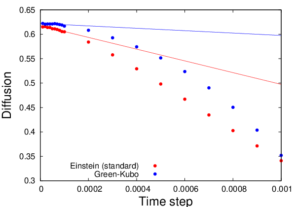
Error estimates for the diffusion coefficients are gathered in Figure 7. For small time steps $\Delta t$, the error in the self-diffusion is linear in $\Delta t$, while nonlinearities appear for larger time steps. The continuous lines are linear fits obtained over the values corresponding to the 10 smallest time steps. As in the simple example discussed in the previous section, estimates obtained with Green-Kubo’s formula seem more reliable than those obtained with Einstein’s formula. Note also that, in accordance with Theorem 1, the self-diffusion is between 0 and 1 in all cases for sufficiently small time-steps.

The idea is to rewrite the part of the additive functional involving $-\nabla V(q_{t})$ as an approximate martingale. To this end, we introduce the solutions $\Phi_{0}=(\Phi_{0,1},..,\Phi_{0,dN})$ of the following Poisson equations

(30)

$$\mathcal{L}\Phi_{0,j}=-\nabla_{q_{j}}V.$$

In view of the resolvent estimate (6), the functions $\Phi_{0,j}$ are well defined elements of $\widetilde{L}^{2}(\mu)$ since

$$\int_{\mathcal{M}}\nabla V\,d\mu=\frac{1}{Z}\int_{\mathcal{M}}\nabla V\,\mathrm{e}^{-\beta V}=-\frac{1}{Z}\int_{\mathcal{M}}\nabla\left(\mathrm{e}^{-\beta V}\right)=0.$$

In addition, by elliptic regularity, the functions $\Phi_{0,j}$ are smooth. By Ito’s lemma, we therefore obtain

$$d\Phi_{0,j}(q_{t})=\mathcal{L}\Phi_{0,j}(q_{t})dt+\sqrt{2}\nabla\Phi_{0,j}(q_{t})\cdot dW_{t},$$

so that the integrated displacement from the origin can be rewritten as

(31)

$$Q_{t}-Q_{0}=-\int_{0}^{t}\nabla V(q_{s})\,ds+\sqrt{2}\,W_{t}=\Phi_{0}(q_{t})-\Phi_{0}(q_{0})+\sqrt{2}\int_{0}^{t}\Big(\mathrm{Id}-\nabla\Phi_{0}(q_{s})\Big)dW_{s}.$$

Since $\Phi_{0}$ is bounded, $(\Phi_{0}(X_{t})-\Phi_{0}(X_{0}))/\sqrt{t}$ uniformly vanishes as $t$ goes to infinity. The long time behavior of the process $F^{T}(Q^{\varepsilon}_{t}-Q^{\varepsilon}_{0})/\sqrt{t}$ (for a given direction $F\in\mathbb{R}^{dN})$ is therefore determined by the martingale

$$\mathscr{M}^{F,\varepsilon}_{t}=\varepsilon\sqrt{\frac{2}{t}}\int_{0}^{t/\varepsilon^{2}}\Big(F-\nabla\left(F^{T}\Phi_{0}(q_{s})\right)\Big)\cdot dW_{s},$$

whose quadratic variation is

$$\left\langle\mathscr{M}^{F,\varepsilon}\right\rangle_{t}=\frac{2\varepsilon^{2}}{t}\int_{0}^{t/\varepsilon^{2}}|F|^{2}-2\nabla\left(F^{T}\Phi_{0}(q_{s})\right)\cdot F+\left|\nabla\left(F^{T}\Phi_{0}(q_{s})\right)\right|^{2}\,ds.$$

The ergodic properties of the diffusion process $q_{t}$ allow to prove that

	$\displaystyle F^{T}\mathscr{D}F=\lim_{t\to+\infty}\left\langle\mathscr{M}^{F,\varepsilon}\right\rangle_{t}$	$\displaystyle=2\int_{\mathcal{M}}|F|^{2}-2\nabla\left(F^{T}\Phi_{0}\right)\cdot F+\left|\nabla\left(F^{T}\Phi_{0}\right)\right|^{2}\,d\mu$
		$\displaystyle=2\int_{\mathcal{M}}|F|^{2}-2\left(F^{T}\Phi_{0}\right)\left(F^{T}\nabla V\right)+\mathcal{L}\left[\left(F^{T}\Phi_{0}\right)\right]\left(F^{T}\Phi_{0}\right)\,d\mu$
(32)			$\displaystyle=2\int_{\mathcal{M}}|F|^{2}-\left(F^{T}\Phi_{0}\right)\left(F^{T}\nabla V\right)\,d\mu=2F^{T}\left(\mathrm{Id}+\int_{\mathcal{M}}\mathcal{L}^{-1}\left(\nabla V\right)\otimes\nabla V\,d\mu\right)F$

where, to pass from the first to the second line, we have used an integration by parts to transform the second term in the integral and (4) for the third one, while the two last equalities follow from the definition of $\Phi_{0}$. At this stage, we note that $F^{T}\mathscr{D}F=0$ implies that the integrand of the first equality vanishes almost everywhere, which, by a Cauchy-Schwarz inequality, in turn implies that $\nabla\left(F^{T}\Phi_{0}\right)$ is proportional to $F$. This is however impossible since $F$ is not the gradient of a periodic function, and we therefore conclude that $\mathscr{D}$ is positive definite. In addition, the last expression shows that $\mathscr{D}\leqslant 2\mathrm{Id}$ since $-\mathcal{L}^{-1}$ is a positive operator (replace $\varphi$ by $\mathcal{L}^{-1}\phi$ in (5)).

Since $-\mathcal{L}$ has a positive spectral gap on $L^{2}(\mu)$ (see (5)), we can write the following operator equality on $\widetilde{L}^{2}(\mu)$ :

$$\mathcal{L}^{-1}=-\int_{0}^{+\infty}\mathrm{e}^{t\mathcal{L}}\,dt.$$

Therefore, for general functions $\psi,\varphi$ with vanishing average with respect to $\mu$,

(33)

$$\int_{0}^{+\infty}\mathbb{E}\Big[\psi(q_{t})\,\varphi(q_{0})\Big]dt=\int_{\mathcal{M}}\left(-\mathcal{L}^{-1}\psi\right)\varphi\,d\mu.$$

Combining this result with (32) leads to the expression (9) of the diffusion matrix $\mathscr{D}$. To prove the convergence of the processes, two arguments should be made precise (see [17] for an elementary account):

1. (i)

   the convergence of the finite-dimensional laws, which can be obtained very simply here by considering the exponential martingales

   $$\exp\left[\mathrm{i}\theta\left(\mathscr{M}_{t}^{F,\varepsilon}-\mathscr{M}_{s}^{F,\varepsilon}\right)+\frac{\theta^{2}}{2}\Big(\left\langle\mathscr{M}^{F,\varepsilon}\right\rangle_{t}-\left\langle\mathscr{M}^{F,\varepsilon}\right\rangle_{s}\Big)\right],$$

   which are such that the conditional expectations converge to those of a Brownian motion as $\varepsilon\to 0$:

   $$\lim_{\varepsilon\to 0}\mathbb{E}\left(\left.\exp\left[\mathrm{i}\theta\left(\mathscr{M}_{t}^{F,\varepsilon}-\mathscr{M}_{s}^{F,\varepsilon}\right)+\frac{\theta^{2}}{2}\Big(\left\langle\mathscr{M}^{F,\varepsilon}\right\rangle_{t}-\left\langle\mathscr{M}^{F,\varepsilon}\right\rangle_{s}\Big)\right]\right|\,\mathcal{F}_{s/\varepsilon^{2}}\right)=\exp\left(-\frac{\theta^{2}}{2}(t-s)F^{T}\mathscr{D}F\right),$$

   $\mathcal{F}_{s/\varepsilon^{2}}$ denoting the filtration of events until the time $s/\varepsilon^{2}$. Finite-dimensional laws are then obtained by a simple induction, as made precise in [1, 17] for instance.

2. (ii)

   the tightness of the process, proved using Prohorov’s criterion (see for instance [2]):

   $$\forall\alpha,\tau>0,\qquad\lim_{\delta\to 0}\limsup_{\varepsilon\to 0}\mathbb{P}\left(\sup_{\begin{subarray}{c}|t-s|<\delta\\ 0\leqslant s<t\leqslant\tau\end{subarray}}\left|F^{T}\Big(Q_{t}^{\varepsilon}-Q_{s}^{\varepsilon}\Big)\right|\geqslant\alpha\right)=0.$$

   This criterion is satisfied in view of the tightness of the martingale $\mathscr{M}^{F,\varepsilon}_{t}$, itself easily obtained using Doob’s inequality (see [17]).

We first determine the magnitude of the acceptance probability in the Metropolis algorithm, which reads

$$R_{\Delta t}(q^{n},\widetilde{q}^{n+1})=\min\left(1,\mathrm{e}^{-\alpha_{\Delta t}(q^{n},\widetilde{q}^{n+1})}\right),$$

with

	$\displaystyle\alpha_{\Delta t}(q,q^{\prime})$	$\displaystyle=V(q^{\prime})-V(q)+\frac{1}{4{\Delta t}}\left[\left(q-q^{\prime}+{\Delta t}\nabla V(q^{\prime})\right)^{2}-\left(q^{\prime}-q+{\Delta t}\nabla V(q)\right)^{2}\right]$
		$\displaystyle=V(q^{\prime})-V(q)-\frac{1}{2}\left\langle q^{\prime}-q,\nabla V(q^{\prime})+\nabla V(q)\right\rangle+\frac{{\Delta t}}{4}\left(|\nabla V(q^{\prime})|^{2}-|\nabla V(q)|^{2}\right).$

Using the following expansions (with integral remainders)

	$\displaystyle V(q^{\prime})-V(q)$	$\displaystyle=\left\langle\nabla V(q),q^{\prime}-q\right\rangle+\frac{1}{2}(q^{\prime}-q)^{T}\left[\nabla^{2}V(q)\right](q^{\prime}-q)+\frac{1}{6}D^{3}V(q)\Big((q^{\prime}-q)^{\otimes 3}\Big)$
(34)			$\displaystyle\ \ \ +\frac{1}{6}\int_{0}^{1}(1-t)^{3}D^{4}V\big((1-t)q+tq^{\prime}\big)\Big((q^{\prime}-q)^{\otimes 4}\Big)\,dt,$
	$\displaystyle\nabla V(q^{\prime})$	$\displaystyle=\nabla V(q)+\nabla^{2}V(q)(q^{\prime}-q)+\frac{1}{2}D^{3}V(q)\Big((q^{\prime}-q)^{\otimes 2}\Big)$
		$\displaystyle\ \ \ +\frac{1}{2}\int_{0}^{1}(1-t)^{2}D^{3}V\big((1-t)q+tq^{\prime}\big)\Big((q^{\prime}-q)^{\otimes 3}\Big)\,dt,$

a simple computation shows that

(35)

$$\alpha_{\Delta t}(q^{n},\widetilde{q}^{n+1})={\Delta t}^{3/2}\xi\left(q^{n},G^{n}\right)+{\Delta t}^{2}\widetilde{\xi}_{\Delta t}(q^{n},G^{n}),$$

where

(36)

$$\xi(q,G)=-\frac{\sqrt{2}}{6}D^{3}V(q)\Big(G^{\otimes 3}\Big)+\frac{\sqrt{2}}{2}\nabla V(q)^{T}\nabla^{2}V(q)G,$$

while there exists a constant $C>0$ such that $\left|\widetilde{\xi}_{\Delta t}(q,G)\right|\leqslant C(1+|G|^{6})$ for any $0\leqslant{\Delta t}\leqslant 1$. We next use the inequality

$$x_{+}-\frac{x_{+}^{2}}{2}\leqslant 1-\min(1,\mathrm{e}^{-x})\leqslant x_{+},\qquad x_{+}=\max(0,x),$$

obtained by distinguishing the cases $x\leqslant 0$ and $x\geqslant 0$. This shows that

(37)

$$R_{\Delta t}(q^{n},\widetilde{q}^{n+1})=1-{\Delta t}^{3/2}\xi_{+}\left(q^{n},G^{n}\right)+{\Delta t}^{2}\widehat{\xi}_{\Delta t}(q^{n},G^{n}),$$

with $\xi_{+}(q,G)=\max(0,\xi(q,G))$ and where $\left|\widehat{\xi}_{\Delta t}(q,G)\right|\leqslant C(1+|G|^{12})$. The estimate on the average acceptance rate (17) is obtained by taking the expectation over all possible realizations of $G^{n}$, with the definition

$$\overline{\xi}(q)=\mathbb{E}_{G}\Big(\xi_{+}(q,G)\Big).$$

References

• [1] A. Bensoussan, J.-L. Lions, and G. Papanicolaou. Asymptotic analysis for periodic structures. AMS Chelsea Publishing, 2011.
• [2] P. Billingsley. Convergence of Probability Measures. Wiley Series in Probability and Statistics, 1999.
• [3] N. Bou-Rabee, A. Donev, and E. Vanden-Eijnden. Metropolis integration schemes for self-adjoint diffusions. Multiscale Model. Sim., 12(2):781–831, 2014.
• [4] N. Bou-Rabee and M. Hairer. Nonasymptotic mixing of the MALA algorithm. IMA J. Numer. Anal., 33:80–110, 2013.
• [5] N. Bou-Rabee and E. Vanden-Eijnden. Pathwise accuracy and ergodicity of metropolized integrators for SDEs. Commun. Pure Appl. Math., 63(5):655–696, 2009.
• [6] N. Bou-Rabee and E. Vanden-Eijnden. A patch that imparts unconditional stability to explicit integrators for Langevin-like equations. J. Comput. Phys., 231:2565–2580, 2012.
• [7] M. Hairer and J. C. Mattingly. Yet another look at Harris’ ergodic theorem for Markov chains. In Seminar on Stochastic Analysis, Random Fields and Applications VI, volume 63 of Progr. Probab., pages 109–117. Birkhäuser/Springer, 2011.
• [8] W. K. Hastings. Monte Carlo sampling methods using Markov chains and their applications. Biometrika, 57:97–109, 1970.
• [9] D. M. Heyes and A. C. Brańka. Monte Carlo as Brownian dynamics. Mol. Phys., 94(3):447–454, 1998.
• [10] M. Jardat. Modélisation Brownienne des solutions. Habilitation thesis, 2005.
• [11] M. Jardat, O. Bernard, P. Turq, and G. R. Kneller. Transport coefficients of electrolyte solutions from Smart Brownian dynamics simulations. J. Chem. Phys., 110(16):7993–7999, 1999.
• [12] B. Leimkuhler, Ch. Matthews, and G. Stoltz. The computation of averages from equilibrium and nonequilibrium Langevin molecular dynamics. Accepted for publication in IMA J. Numer. Anal. (2014)
• [13] T. Lelièvre, M. Rousset, and G. Stoltz. Free-energy Computations: A Mathematical Perspective. Imperial College Press, 2010.
• [14] J. C. Mattingly, A. M. Stuart, and D. J. Higham. Ergodicity for SDEs and approximations: locally Lipschitz vector fields and degenerate noise. Stoch. Proc. Appl., 101(2):185–232, 2002.
• [15] N. Metropolis, A. W. Rosenbluth, M. N. Rosenbluth, A. H. Teller, and E. Teller. Equations of state calculations by fast computing machines. J. Chem. Phys., 21(6):1087–1091, 1953.
• [16] G. N. Milstein and M. V. Tretyakov. Stochastic Numerics for Mathematical Physics. Scientific Computation. Springer, 2004.
• [17] S. Olla. Homogenization of diffusion processes in random fields, 1994. Lecture notes from Ecole polytechnique, www.ceremade.dauphine.fr/∼\simolla/lho.ps.
• [18] G. O. Roberts and R. L. Tweedie. Exponential convergence of Langevin distributions and their discrete approximations. Bernoulli, 2(4):341–363, 1996.
• [19] P. J. Rossky, J. D. Doll, and H. L. Friedman. Brownian dynamics as smart Monte Carlo simulation. J. Chem. Phys., 69(10):4628–4633, 1978.