Fast prediction of deterministic functions using sparse grid experimental designs
Matthew Plumlee11footnotemark:
1
11footnotemark:
1
Georgia Institute of Technology, Atlanta, Georgia
(mplumlee@gatech.edu)
Matthew Plumlee is currently a Ph.D. candidate at the H. Milton Stewart School of Industrial and Systems Engineering at the Georgia Institute of Technology. This document is in-press at the Journal of the American Statistical Association. A MATLAB package released along with this document is available at http://www.mathworks.com/matlabcentral/fileexchange/45668-sparse-grid-designs.
Abstract
Random field models have been widely employed to develop a predictor of an expensive function based on observations from an experiment. The traditional framework for developing a predictor with random field models can fail due to the computational burden it requires. This problem is often seen in cases where the input of the expensive function is high dimensional. While many previous works have focused on developing an approximative predictor to resolve these issues, this article investigates a different solution mechanism. We demonstrate that when a general set of designs is employed, the resulting predictor is quick to compute and has reasonable accuracy. The fast computation of the predictor is made possible through an algorithm proposed by this work. This paper also demonstrates methods to quickly evaluate the likelihood of the observations and describes some fast maximum likelihood estimates for unknown parameters of the random field. The computational savings can be several orders of magnitude when the input is located in a high dimensional space. Beyond the fast computation of the predictor, existing research has demonstrated that a subset of these designs generate predictors that are asymptotically efficient. This work details some empirical comparisons to the more common space-filling designs that verify the designs are competitive in terms of resulting prediction accuracy.
Keywords: Computer experiment; Gaussian process; Simulation experiment; High dimensional input; Large-scale experiment
1 Predicting expensive functions
Consider a case where a deterministic output can be observed corresponding to a controllable input and the cost of an observation is expensive or at least non-negligible. Analysis that requires a huge number of evaluations of the expensive function for different inputs can prove impractical. This paper examines a method to avoid the impracticality problem with the creation of a function that behaves similarly to the function of interest with a relatively cheap evaluation cost. We term this cheap function a predictor as it can closely match the output for an untried input. The predictor can be used in place of the expensive function for subsequent analysis.
Beginning in the 1980s, research has emphasized the use of Gaussian process models to construct predictors of the expensive function (Sacks et al., 1989). This method, often referred to as kriging, sprouted in geostatistics (Matheron, 1963) and is considered the standard approach to study expensive, deterministic functions. A great deal of attention has been paid to this method and important variations over the last two decades because of the increased emphasis on computer simulation (Kennedy and O’Hagan, 2001, Santner et al., 2003, Higdon et al., 2008, Gramacy and Lee, 2008). The major objectives for analysis outlined in Sacks et al. (1989) have remained basically constant: predict the output given inputs, optimize the function, and adjust inputs of the function to match observed data. Recently, researchers have studied a fourth objective of computing the uncertainty of the output when inputs are uncertain, a topic in the broad field of uncertainty quantification. All of these objectives can be achieved through the use of a predictor, though sometimes under different names, e.g. emulator or interpolator.
1.1 Predictors and Gaussian process modeling
As summarized in Sacks et al. (1989), a predictor is constructed by assuming that the output, termed , is a realization of an unknown, random function of a dimensional input in a space . One notational comment: each element in an input is denoted , i.e. , while sequences of inputs are denoted with subscripts, e.g. . To construct a predictor, an experiment is performed by evaluating the function for a given experimental design (a sequence of inputs), , creating a vector of observations . The value of is known as the sample size of the experimental design. A smaller sample size represents a less expensive design.
After observing these input/output pairs, a predictor is then built by finding a representative function based on the observations. The often adopted approach treats the unknown function as the realization of a stochastic process. Specifically, is a realization of a random function which has the density of a Gaussian process. The capitalization of the output indicates a random output while the lower case indicates the observed realization. We denote the Gaussian process assumption on a random function as
where is the mean function and is a function such that for all possible .
A typical assumption on the covariance structure is a separable covariance, defined as for all . The functions are covariance functions defined when the input is one dimensional. The value of is proportional to the covariance between two outputs corresponding to inputs where only the th input differs from to . The results in this paper require this covariance structure to hold, but no other assumptions are needed for and . Section 5 discusses estimating the aforementioned mean and covariance functions using the observations when they are unknown. For now, we consider these functions known for simplicity of exposition.
Our goal is to predict an unobserved output at an untried input given . The commonly used predictor of is
| (1) |
where is a vector of weights and . In general, is given by the following relation
where and is the covariance matrix where the element in the th row and th column is . This predictor, , is commonly used because it is both the mean and median of the predictive distribution of given . This property implies is optimal among the class of both linear and nonlinear predictors of with respect to the quadratic and absolute loss functions.
1.2 Focus of the paper
The above approach, when applied in a direct manner, can become intractable because the inversion of the covariance matrix is an expensive operation in terms of both memory and processing. Direct inversion can also induce numerical errors due to limitations of floating point mathematical computations (Wendland, 2005, Haaland and Qian, 2011). Previous research has focused on changing the matrix to a matrix that is easier to invert, therefore making the computation of faster (Furrer et al., 2006, Cressie and Johannesson, 2008, Banerjee et al., 2008). We term this an approximation because this can degrade predictive performance, though sometimes only slightly.
In this work, we forgo approximations and investigate a new approach to resolve this problem: by restricting ourselves a general class of designs, accurate non-approximative predictors can be with found with significantly less computational expense. This class of experimental designs is termed sparse grid designs and is based on the structure of eponymic interpolation and quadrature rules. Sparse grid designs (Smolyak, 1963) have been used with in conjunction with polynomial rules (Wasilkowski and Woźniakowski, 1995, Barthelmann et al., 2000, Xiu and Hesthaven, 2006, Nobile et al., 2008, Xiu, 2010), but these designs have not gained popularity among users of random field models. Here, we encourage the use of sparse grid designs by demonstrating computational procedures to be used with these designs where the predictor can be computed very quickly.
Section 2 will briefly describe two broad types of existing designs and identify deficiencies of those existing types. Section 3 will explain the definition of sparse grid designs and then the following sections will discuss three important topics:
- •
Section 4 explains how we can exploit the structures used in building sparse grid designs to achieve extreme computational gains when building the predictor. Our algorithm computes by inverting several small matrices versus one large matrix. This algorithm is derived from the result that can be written as the tensor product of linear operators, see theorem 2 in appendix B.
- •
- •
Section 6 illustrates that sparse grid designs perform well even when the input is high dimensional. We conduct empirical comparisons that demonstrate good performance of these designs which supports the positive asymptotic arguments proven previously (Temlyakov, 1987).
Section 7 will offer some discussions on the role of these designs and the creation of optimal sparse grid designs.
2 Space-filling and lattice designs
This section will briefly discuss existing research on space-filling and lattice designs. The space-filling category includes the popular Latin hypercube designs. Lattice designs are a specific class of designs where each design is a Cartesian product of one dimensional designs. Visual examples are given in figure 1 and they are contrasted with an example of a sparse grid design which will be explained in section 3.

2.1 Space-filling designs: Efficient predictors but difficult computation
Current research has emphasized the design of points that are space-filling (see figure 1 (a) and (b)). Designs of this type are often scattered, meaning they are not necessarily located on a lattice. The major focus has been on Latin hypercube designs (McKay et al., 1979), seen in figure 1 (a), and research has produced a swell of variations, e.g. Tang (1993), Owen (1994), Morris and Mitchell (1995), Ye (1998), Joseph and Hung (2008). These designs have been shown to perform well in many prediction scenarios and are often considered the standard method of designing computer experiments for deterministic functions.
However, space-filling designs experience significant difficulties when the input is high dimensional, i.e. . In these cases, one requires a large sample size to develop an accurate predictor. This in turn makes the matrix very large, meaning is difficult to compute through inversion of . This has motivated the research into approximate predictors discussed in section 1.2 that can be used with space-filling designs.
2.2 Lattice designs: Easy computation but inefficient predictors
One of the simplest forms of an experimental design is a lattice design, also known as a grid. This is defined as where each is a set of one dimensional points we term a component design. For a set and , the Cartesian product, denoted , is defined as the set of all ordered pairs where and . If the number of elements in is , then the sample size of a lattice design is .
Let the covariance be as stated in section 1.1, . When a lattice design is used, the covariance matrix takes the form of a Kronecker product of matrices: , where is a matrix composed of elements for all . A useful property of Kronecker products can be derived using only the definition of matrix multiplication and the commutativity of scalar multiplication: if and then (when matrices are appropriately sized). This immediately implies that if and are both invertible matrices, . Thus, if a lattice design is used,
which is an extremely fast algorithm because are sized matrices. Many authors have noted the power of using lattice designs for fast inference for these types of models (O’Hagan, 1991, Bernardo et al., 1992). Say that we have a symmetric design where for all and . Computing requires inversion of sized matrices which are much smaller than the sized matrix . Because inversion of an size matrix requires arithmetic operations, inverting multiple small matrices versus one large one yields significant computational savings.
While lattice designs are extremely simple and result in fast-to-compute predictors, these are wholly impractical for use in high dimensions. First, lattices are grossly inefficient as experimental designs when the dimension is somewhat large (), which will be demonstrated in section 6. Also, the sample size of a lattices designs, , is extremely inflexible regardless of the choice of . At minimum , and then even for a reasonable number of dimensions the size of the design can become quite large. When the smallest possible design size is over .
3 Sparse grid designs
This section will discuss the construction of sparse grid experimental designs which are closely associated with sparse grid interpolation and quadrature rules. To build these designs first specify a nested sequence of one dimensional experimental designs for each denoted , where , and . Designs defined for a single dimension, e.g. , are termed component designs in this work. The nested feature of these sequences is important for our case. The general literature related to sparse grid rules does not require this property. Here, it is necessary for the stated results to hold.
Sparse grid designs are therefore defined as
| (2) |
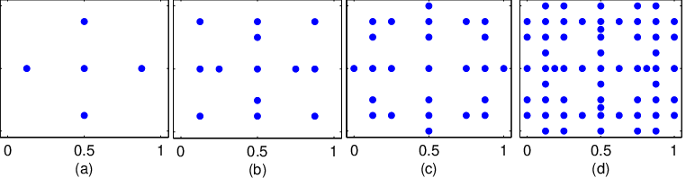
where is an integer that represents the level of the construction and . Here we use the overhead arrow to distinguish the vector of indices, from a scalar index. Increasing the value of results in denser designs. Figure 3 illustrates the construction of the two dimensional designs seen in figure 3. The details of the component designs can be seen in appendix A.

Unlike many other design alternatives, sparse grid designs are not defined via a given sample size. The sample size of the resulting sparse grid design is a complicated endeavor to compute a-priori. After the dimension and level of construction , a major contributing factor to the sample size, , is the sizes of the component designs. The sample size of a sparse grid design is given by
where . Table 1 presents some shortcut calculations of the sample size along with some bounds when for all and .
| Bound on | ||
|---|---|---|
| if | ||
The proper selection of the points in the component designs is essential to achieving good performance of the overall sparse grid design. Establishing good component designs can lead to a good sparse grid design, but interaction between dimensions is an important consideration.
4 Fast prediction with sparse grid designs
This section will propose an algorithm that shows the major advantage of sparse grid designs: the availability of fast predictors. Appendix B justifies the proposed algorithm by describing a predictor in the form of a tensor product of linear maps and then theorem 2 demonstrates that conjectured predictor is the same as .
Here we show how to build the weight vector, , by inverting covariance matrices associated with the component designs which are relativity small compared to . Therefore, our proposed method results in a faster computation of than a method that computes from direct inversion of when is large. This is the same mechanism that is used to construct fast predictors with lattice designs. But unlike lattice designs, we show sparse grid designs perform well in cases where the input is high dimensional in section 6.
Algorithm 1 lists the proposed algorithm for computing . In the algorithm, the matrices are composed of elements , for all . Also, the vectors , and denote subvectors of , and at indices corresponding to for all .
| Initialize |
| For all |
Another important feature of predictors in general is the presence of a predictive variance,
where the subscript on the expectation implies we condition on that case. As noted before, computation of is an undesirable operation. Luckily, this operation can be avoided by using sparse grid designs. As demonstrated in appendix C, when employing a sparse grid design the predictive variance is given by
| (3) |
where and is defined as the expected squared prediction error in one dimension with covariance and design . After substituting known relations, we have that
where the elements of the vector are for all .
Observation 1.
Some exact comparisons are helpful to understand how fast algorithm 1’s computation of is compared to the traditional method. Using the same settings as section 6.1 with and , the computation of took seconds with the proposed algorithm and the traditional method of computing by inverting took seconds. In a much larger example with ( and ), computing using the proposed algorithm took seconds. If we assume the cost of prediction scales at the rate of matrix inversion, , then computing using the traditional method of inverting with a design size of would take approximately 81 days to compute.
5 Fast prediction with unknown parameters
The previous section assumed that both mean, , and covariance, , are exactly known. This is often not assumed in practical situations. Instead, these functions are given general structures with unknown parameters which we denote . Two major paradigms exist for prediction when is unknown: (i) simply use an estimate for based on the observations and predict using (1) or (ii) Bayesian approaches (Santner et al., 2003). For either method, the typical formulae require computation of both the determinant and inverse of , which are costly when is large. This section develops the methods to avoid these computations. For expositional simplicity, this section will outline the first method and leave the full Bayesian method for future work.
The estimate of we consider will be the maximum likelihood estimate (MLE), which is denoted . We therefore term the predictor that uses this estimate as the MLE-predictor, which will be used for comparisons in section 6.2. We first explain the typical general structures of and in section 5.1 and then we describe the traditional forms of the estimate and problems with them in section 5.2. Section 5.3 then explains fast methods to find in this setting.
5.1 General setting
The structures of , and in this section are borrowed from Santner et al. (2003) and are widely employed. We assume that the mean is a linear combination of basis functions, , and the covariance function is scaled such that , where is a correlation function and represents the variance of . The parameter is a general parameter or group of parameters that can represent unknown aspects of that affect the lengthscale and differentiability of the realized response . We now have the following case
where is the set of unknown parameters.
5.2 Traditional computation of the MLE
The logarithm of the probability density of the observations with , called the log-likelihood, is given by (up to a constant)
where represents the determinant of a matrix , is the correlation matrix of when parameter is used, , and
Our goal is to solve the optimization problem
There are closed form maximum likelihood estimates for both and given which we denote and . They are
and
Then, is found by generic numerical maximization, i.e.
The problem with using these methods directly is that and require inversion of the matrix . Additionally, still contains the term , which is often as cumbersome as finding . The remainder section proposes alternatives to these methods that are faster. Specifically, we will be able to compute , and without ever storing or operating directly on .
5.3 Proposed fast computation of the MLE
To introduce our fast-to-compute maximum likelihood estimate, we first describe a generalization of algorithm 1 seen in algorithm 2. Algorithm 2 computes
where is any matrix and is any positive integer. The notation “” implies we have a separable covariance with each covariance function being represented by . The computations in algorithm 2 do not require the direct inversion of and therefore avoid the major computational problems of the traditional method. The validity of algorithm 2 is implied by the validity of algorithm 1.
| Initialize as an matrix with all entries. |
| For all |
| Output . |
Now we can establish our maximum likelihood estimates for and that do not require inversion of the matrix . For a given ,
and
The last step to find the MLE requires maximization of with respect to . This expression contains the term which, as mentioned before, is expensive to compute. Therefore, we demonstrate the following theorem related to the expression of the determinant that only involves determinants of component covariance matrices, . The proof lies in the appendix.
Theorem 1.
If , then
where for all .
By using as the covariance function in the formula in the above theorem, we gain an expression for without directly computing the determinant of an matrix. Once is found, this gives us .
6 Prediction performance comparisons
Thus far, this paper has established that we can build predictors quickly when sparse grid designs are used. However, an issue of critical importance is how well the resulting predictors perform. This section seeks to compare the predictive performance resulting from sparse grid designs to the more common designs discussed in section 2. Our core findings can be summarized as follows: (i) both sparse grid and space-filling designs outperform lattice designs, (ii) sparse grid designs appear competitive with space-filling designs for smooth functions and inferior to space-filling designs for very rough functions, and (iii) the time taken to find the MLE-predictor using sparse grid designs can be orders of magnitude less than the time taken using the traditional methods.
Before we begin numerical comparisons, it might be helpful to take a historical look at sparse grid designs. The prevalence of sparse grid designs in the numerical approximation literature can be owed to the demonstrated efficiency of the designs even when the input is of high dimension. It has been shown if , using sparse grid designs with component designs of the form is an asymptotically efficient design strategy under the symmetric separable covariance structure (Temlyakov, 1987, Woźniakowski, 1992, Ritter et al., 1995). These designs are also known as hyperbolic cross points. The key point discovered in the previous analysis is that sparse grid designs are asymptotically efficient regardless of dimension and lattice designs become increasingly inefficient as the dimension grows large. Therefore, we anticipate that sparse grid designs outperform lattices in high dimensions.
The sparse grid designs used in this section were constructed from component designs that are symmetric across dimensions and details of the component designs are in appendix A. These appeared to be at least competitive if not superior to hyperbolic cross points in a simulation study comparable to section 6.1. The space-filling designs were constructed by using the scrambled Sobol sequence described in Matoušek (1998). Maximin Latin hypercube designs that were generated via the R package hs produced inferior distance metrics for arge sample sizes but the same conclusions as the ones presented in this section. The lattice design designs used for comparison in section 6.1 were , , and .
6.1 Comparison via average prediction error
This subsection will investigate the mean square prediction error resulting from various experimental designs when the mean and covariance structures are known. This can be thought of as the average mean squared prediction error over all possible sample paths, , drawn from a Gaussian process with a specified covariance function. Furthermore, we seek to examine the impact of the smoothness of on the effectiveness of the design strategies. To allow for the introduction of varying levels of smoothness, this section will use the Matérn class of covariance functions,
| (4) |
where is the modified Bessel function of order and . The use of this covariance class allows us to independently adjust a smoothness parameter , where the sample paths are times differentiable (Handcock and Stein, 1993). For simplicity, this subsection uses homogenous covariance in every dimension. For the case when and , figure 4 compares the average root mean squared prediction error (RMSPE) resulting from the design strategies computed through Monte Carlo samples on . Note if , the RMSPEs for the space-filling designs were not recorded due to numerical instability when inverting the large covariance matrix.
Figure 4

indicates sparse grid designs yield superior performance to lattice designs. The results also demonstrate the similarity of the sparse grid designs and space-filling designs in cases of the existence of at least one derivative. However, sparse grid designs appear inferior to the space-filling designs if the sample path has almost surely no differentiability.
6.2 Comparison via deterministic functions
This section will compare the performance of sparse grid designs and space-filling designs on a set of deterministic test functions. For both methods, we assume the mean and covariance structures of the deterministic functions are unknown and use the MLE-predictor. For , we use a constant mean structure, , and for the covariance function we use a scaled Matérn with and single lengthscale parameter for all dimensions . This analysis will report the median absolute prediction error, which is more robust to extreme observations compared to the mean square prediction error. The median absolute prediction error will be estimated by the sample median of the absolute prediction error at randomly selected points in the input space. We consider the following functions: Franke’s function (Franke, 1982), the Borehole function (Morris et al., 1993), the product peak function given by , the corner peak function given by
and the Rosenbrock function given by
With the exception of the Borehole function, all domains are (the Borehole function was scaled to the unit cube). For the space-filling designs, designs sizes were restricted to cases where memory constraints in MATLAB were not violated on the author’s computer.
Figure 5

presents the results of the study. Most functions were similarly estimated using either design strategy. While Franke’s function has significantly more bumps and ridges compared to the other functions, making it more difficult to estimate, good prediction of Franke’s function based on few observations is possible because the input to the function is located in a dimensional space. At the other extreme, while the corner peak function is smooth, estimating the function when is a very challenging task. Using a space-filling design of size does not do an adequate job of estimating the function as it produces median absolute prediction error of about times more than the best that can be achieved using a sparse grid design with a much larger design size. Similar effects are seen when attempting to estimate the Rosenbrock function in dimensions.
Figure 6

compares the computational time needed to find both and the weights using both the traditional method and the proposed method for the MLE-predictors used to produce figure 5. The method to find the MLE-predictor was described in section 5. There was three cases where the cost of the traditional algorithm with a design size of less than was more than the proposed algorithm with a design size of nearly a million. While the design sizes attempted for the traditional algorithm were limited for memory and numerical stability reasons, some extrapolation emphasizes the problem with using the traditional algorithm on experiments with huge sample sizes. A sample size of a million points would require roughly seconds, or days, to find the MLE-predictor. By using a sparse grid design, we are able to compute the MLE-predictor based on a million observations in a fraction of that time, about 15 minutes ( seconds).
7 Discussion
The proposed sparse grid designs deviate from the traditional space-filling framework and utilize lattice structures to construct efficient designs. Sparse grid designs appear to be competitive with common space-filling designs in terms of prediction, but space-filling designs appear to outperform sparse grid designs in simulations where the underlying function has no differentiability. Based on the discussions at the end of section 6.1, these early results may extend to cases that can be classified as rough functions.
Sparse grid designs are an enormously flexible framework and this work has not yet realized their full potential. A topic not discussed at length in this work are optimal sparse grid designs, which might be able to close any small performance gaps between sparse grid and space-filling designs. Optimality is dictated by the choice of design criteria, which has previously focused on distance measures such as the minimum distance between any two design points. When the sample size grows large, this can become an expensive metric to compute as it requires arithmetic operations. Therefore, using the shortcut calculations for integrated prediction error, see equation (3), or maximum entropy, see theorem 1, might be faster criteria to compute (see Sacks et al. (1989) for more information on these criteria).
A problem not yet solved using the proposed designs occurs when the covariance function is not separable. The study of these situations merits more work. As an example, if the sample path contains distinct areas with differing behavior, the assumption of local separability might be a more apt modeling strategy. Using only local separability assumptions, methods similar to Gramacy and Lee (2008) could be employed with local sparse grid designs that study heterogeneous sections of the function.
Acknowledgments
Special thanks go to C.F.J. Wu, V.R. Joseph, R. Tuo, J. Lee, an anonymous associate editor, and anonymous reviewers for their inspirations and insights on this current revision. This work was partially supported by NSF grant CMMI-1030125 and the ORACLE summer fellowship from Oak Ridge National Laboratories.
Appendices
One notational difference between the body of the paper and these appendices: Since the proofs for theorems 1 and 2 are demonstrated through induction by treating the level of construction and the dimension as variables, we use the indexing for the design , the design size , the index sets and , and the covariance matrix . Also, the symbol means ‘set-minus’, i.e. is the elements in that are not in .
Appendix A Component designs used for the sparse grid designs in this work
The sparse grid design in figure 1, subplot c, was created where , and , and are and respectively for and .
The sparse grid design in figure 3 was created with component designs such that , , , , , , and are , , , , , and respectively for all . These component designs were chosen through an ad-hoc method, but are essentially based on maintaining good spread of points as increases.
Appendix B Proof that algorithm 1 produces correct
The correctness of produced by algorithm 1 is difficult to understand without the use of linear operators, therefore we will rephrase discussed in section 1.1 in terms of a linear operator. Let be a function space of functions that map to . Let be a predictor operator with respect to if where . The following definition explains an optimal predictor operator.
Definition 1.
A predictor operator is termed optimal with respect to and if and
A predictor operator is termed optimal because
is the best linear unbiased predictor of given the observations when is optimal with respect to and (Santner et al., 2003).
In general, the optimal predictor operator is when is the th element in . There are cases where the predictor operator is unique. Therefore, we only need to show a clever form of the optimal predictor operator that agrees with the produced by algorithm 1 to complete our argument.
Now we define a sequence, , of predictor operators, , for each dimension . These are the optimal predictor operators with respect to and when the dimension of the input is and the covariance function is .
To find the desired form of the optimal predictor operator with respect to sparse grid designs, one could guess that the quadrature rule of Smolyak (1963) will be of great use. In our terms, the Smolyak quadrature rule can be interpreted as the predictor operator
| (5) |
where the symbol for linear operators is the tensor product. .
While this form of is known, the optimality of in the situation discussed has not yet to been proved to the author’s knowledge. Wasilkowski and Woźniakowski (1995) study the case where for all and . They show an optimality property with respect to an norm, which they term worst case. Wasilkowski and Woźniakowski go on to state in passing that one could verify that (5) is mean of the predictive distribution and therefore optimal in our setting, but they do not demonstrate it in that work. Here, we formally state and demonstrate this result.
Theorem 2.
The predictor operator is optimal with respect to and . Furthermore, can be written in the form
| (6) |
where and .
The different statements of (5) and (6) are important to note. The predictor operator in (5) is theoretically intuitive as it geometrically explains how we maintain orthogonality as grows and allows for the subsequent proof. However, if we were to attempt to use (5) directly, each term in the sum would require us to sum terms after expansion, which may temper any computational advantages the lattice structure yields. Wasilkowski and Woźniakowski show that (5) can be written of the form (6). This result is simply an algebraic manipulation and requires no conditions regarding optimality, but the result allows us to easily use (5).
Proof of theorem 2
Proof.
Let
where and . We need to show that
Since , the objective function is minimized when the covariance between and values of at all points in is . Thus, we need to show that
for all .
If , the theorem is clearly true for all . Assume that the theorem is true for and all ; we will show that it is true for and . This demonstrates the result by an induction argument.
We have that
| (7) |
Observe that
| (8) |
Since is the optimal predictor operator with respect to and , if . Let
and let . Since sparse grid designs have nested component designs, if , then since . This implies if , then Then (8) can be rewritten as
| (9) |
Also, if then and
which implies
| (10) |
| (11) |
By the induction assumption, the theorem is true for , which means that for and , (7) is equal to zero. Therefore,
This gives us the desired result for ,
Inserting this into (7) yields the major result that (5) is the optimal predictor operator.
In Wasilkowski and Woźniakowski (1995), they demonstrate through combinatorial relations and algebraic manipulations that (5) can be simplified to (6). ∎
Appendix C Proof that (3) is the MSPE
Due to theorem 2,
Because is the optimal predictor operator in one dimension with respect to and , we have
where is defined in section 4.
Lastly, we have that since is an affine map from and follows a Gaussian process, and are jointly multivariate normal. By theorem 2, there is covariance between them. Therefore is independent of and we can condition the expectation on the left-hand-side on without affecting the right-hand-side.
Appendix D Proof of theorem 1
Proof.
If , the theorem is clearly true for all . We now prove this result by induction. Assume the theorem is true for and all .
To demonstrate this result, we require the use of the Schur complement. Let . The Schur complement of with respect to , expressed , is defined by (if is invertible). The determinant quotient property of the Schur complement is . The theorem can be rewritten as
We also require following result:
| (12) |
where and are and sized matrices, respectively.
We will use the notation to denote the submatrix of with respect to the elements which correspond to . Expanding the term with respect the quotient property
| (13) |
Let
Now, observe the elements of that correspond to ,
where is a covariance matrix corresponding to , is a covariance matrix corresponding to , and is the cross covariance. Since and ,
So,
which can be used with (13) to show
Iterating the expansion to yields,
The term outside of the product is the Schur complement of a positive definite matrix with itself, which is an empty matrix. By the Leibniz formula, the determinant is . Therefore,
References
- Banerjee et al. (2008) Banerjee, S., Gelfand, A., Finley, A., and Sang, H. (2008), “Gaussian predictive process models for large spatial data sets,” Journal of the Royal Statistical Society: Series B, 70, 825–848.
- Barthelmann et al. (2000) Barthelmann, V., Novak, E., and Ritter, K. (2000), “High dimensional polynomial interpolation on sparse grids,” Advances in Computational Mathematics, 12, 273–288.
- Bernardo et al. (1992) Bernardo, M. C., Buck, R., Liu, L., Nazaret, W. A., Sacks, J., and Welch, W. J. (1992), “Integrated circuit design optimization using a sequential strategy,” Computer-Aided Design of Integrated Circuits and Systems, IEEE Transactions on, 11, 361–372.
- Cressie and Johannesson (2008) Cressie, N. and Johannesson, G. (2008), “Fixed rank kriging for very large spatial data sets,” Journal of the Royal Statistical Society: Series B, 70, 209–226.
- Franke (1982) Franke, R. (1982), “Scattered data interpolation: tests of some methods,” Mathematics of Computation, 38, 181–200.
- Furrer et al. (2006) Furrer, R., Genton, M. G., and Nychka, D. (2006), “Covariance tapering for interpolation of large spatial datasets,” Journal of Computational and Graphical Statistics, 15.
- Gramacy and Lee (2008) Gramacy, R. B. and Lee, H. K. (2008), “Bayesian treed Gaussian process models with an application to computer modeling,” Journal of the American Statistical Association, 103.
- Haaland and Qian (2011) Haaland, B. and Qian, P. Z. (2011), “Accurate emulators for large-scale computer experiments,” The Annals of Statistics, 39, 2974–3002.
- Handcock and Stein (1993) Handcock, M. and Stein, M. (1993), “A Bayesian analysis of kriging,” Technometrics, 35, 403–410.
- Higdon et al. (2008) Higdon, D., Gattiker, J., Williams, B., and Rightley, M. (2008), “Computer model calibration using high-dimensional output,” Journal of the American Statistical Association, 103.
- Joseph and Hung (2008) Joseph, V. R. and Hung, Y. (2008), “Orthogonal-maximin Latin hypercube designs,” Statistica Sinica, 18, 171–186.
- Kennedy and O’Hagan (2001) Kennedy, M. C. and O’Hagan, A. (2001), “Bayesian calibration of computer models,” Journal of the Royal Statistical Society: Series B (Statistical Methodology), 63, 425–464.
- Matheron (1963) Matheron, G. (1963), “Principles of geostatistics,” Economic geology, 58, 1246–1266.
- Matoušek (1998) Matoušek, J. (1998), “On the -Discrepancy for Anchored Boxes,” Journal of Complexity, 14, 527–556.
- McKay et al. (1979) McKay, M. D., Beckman, R. J., and Conover, W. J. (1979), “Comparison of three methods for selecting values of input variables in the analysis of output from a computer code,” Technometrics, 21, 239–245.
- Morris and Mitchell (1995) Morris, M. D. and Mitchell, T. J. (1995), “Exploratory designs for computational experiments,” Journal of Statistical Planning and Inference, 43, 381–402.
- Morris et al. (1993) Morris, M. D., Mitchell, T. J., and Ylvisaker, D. (1993), “Bayesian design and analysis of computer experiments: use of derivatives in surface prediction,” Technometrics, 35, 243–255.
- Nobile et al. (2008) Nobile, F., Tempone, R., and Webster, C. G. (2008), “A sparse grid stochastic collocation method for partial differential equations with random input data,” SIAM Journal on Numerical Analysis, 46, 2309–2345.
- O’Hagan (1991) O’Hagan, A. (1991), “Bayes–Hermite quadrature,” Journal of Statistical Planning and Inference, 29, 245–260.
- Owen (1994) Owen, A. (1994), “Controlling correlations in Latin hypercube samples,” Journal of the American Statistical Association, 89, 1517–1522.
- Ritter et al. (1995) Ritter, K., Wasilkowski, G., and Woźniakowski, H. (1995), “Multivariate integration and approximation for random fields satisfying Sacks-Ylvisaker conditions,” The Annals of Applied Probability, 5, 518–540.
- Sacks et al. (1989) Sacks, J., Welch, W., Mitchell, T., and Wynn, H. (1989), “Design and analysis of computer experiments,” Statistical Science, 4, 409–423.
- Santner et al. (2003) Santner, T., Williams, B., and Notz, W. (2003), The design and analysis of computer experiments, Springer Verlag.
- Smolyak (1963) Smolyak, S. A. (1963), “Quadrature and interpolation formulas for tensor products of certain classes of functions,” Soviet Math Dokl., 4, 240–243.
- Tang (1993) Tang, B. (1993), “Orthogonal array-based Latin hypercubes,” Journal of the American Statistical Association, 88, 1392–1397.
- Temlyakov (1987) Temlyakov, V. (1987), “Approximate recovery of periodic functions of several variables,” Mathematics of the USSR-Sbornik, 56, 249.
- Wasilkowski and Woźniakowski (1995) Wasilkowski, G. and Woźniakowski, H. (1995), “Explicit cost bounds of algorithms for multivariate tensor product problems,” Journal of Complexity, 11, 1–56.
- Wendland (2005) Wendland, H. (2005), Scattered Data Approximation, Cambridge Monographs on Applied and Computational Mathematics.
- Woźniakowski (1992) Woźniakowski, H. (1992), “Average case complexity of linear multivariate problems I. Theory,” Journal of Complexity, 8, 337–372.
- Xiu (2010) Xiu, D. (2010), Numerical Methods for Stochastic Computations: a spectral method approach, Princeton Univ Pr.
- Xiu and Hesthaven (2006) Xiu, D. and Hesthaven, J. (2006), “High-order collocation methods for differential equations with random inputs,” SIAM Journal on Scientific Computing, 27, 1118.
- Ye (1998) Ye, K. Q. (1998), “Orthogonal column Latin hypercubes and their application in computer experiments,” Journal of the American Statistical Association, 93, 1430–1439.