Self-localized states in species competition
Abstract
We study the conditions under which species interaction, as described by continuous versions of the competitive Lotka-Volterra model (namely the nonlocal Kolmogorov-Fisher model, and its differential approximation), can support the existence of localized states, i.e. patches of species with enhanced population surrounded in niche space by species at smaller densities. These states would arise from species interaction, and not by any preferred niche location or better fitness. In contrast to previous works we include only quadratic nonlinearities, so that the localized patches appear on a background of homogeneously distributed species coexistence, instead than on top of the no-species empty state. For the differential model we find and describe in detail the stable localized states. For the full nonlocal model, however competitive interactions alone do not allow the conditions for the observation of self-localized states, and we show how the inclusion of additional facilitative interactions lead to the appearance of them.
I Introduction
The interactions among the biological entities integrating an ecosystem give rise to surprising emergent behaviors. Competition is one of the most important and ubiquitous of these interactions: if there is an increase in the population of one species, due to the consumption of common resources or shared predators [1], there is a decrease in the growth rate of the others. Because of this interaction it is usually argued that a given ecosystem can host only a limited number of species that should be sufficiently separated from each other in the so-called niche space. This is the -dimensional space whose coordinates (, , …) quantify the traits of the species relevant for the utilization of the resources distributed as a function of these coordinates. The competitive exclusion principle [2] is a formulation of this situation, in which species can not coexist too close in niche space (limiting similarity). Despite this reasoning, however, it should be said that even the most traditional mathematical model of competitive species, the Lotka-Volterra (LV) model [3], is known to allow solutions characterized by a continuous distribution of species [4] under some circumstances (see reviews in [5, 6]). More remarkable in this context are recent results on the LV model (or closely related ones) showing the existence of solutions that do not represent purely continuous coexistence, nor are typical of a limiting similarity situation [7, 8, 9, 5]: clusters of species around particular niche positions well separated from each other and filling out the niche space. For the competitive LV model, these lumped distributions appear due to pattern forming instabilities triggered by the shape of the interaction function [8, 9, 10, 11]. Besides these many-cluster species configurations, an ecologically relevant question is under which conditions solitary clusters of species may appear. These would arise from an evolutionary or random drift towards a particular niche position, or simply from an advantageous initial condition. In this Paper, we address this question in the context of pattern formation in continuous versions of the LV model, both in an integral formulation as in its differential approximation. Our focus is on competitive interactions, but we will be forced to consider also some facilitative (i.e. mutualistic or symbiotic) situations. Through the paper we will keep in mind the situation of species competition in niche space, but we stress that the concepts and type of models used here are equally valid to describe organisms randomly moving in physical space and nonlocally competing for resources with other individuals in their spatial neighborhood [12, 13], or rather in evolutionary situations [14, 15].
A pattern-forming instability or bifurcation is a source of great complexity, and many different scenarios may arise from it. One of the simplest cases is the formation of a periodic structure, that in two or higher dimensions can have different geometries depending on the nature of the nonlinearities. In some cases the bifurcation can be subcritical so that periodic patterns can coexist with homogeneous distributions. In this case localized solutions consisting of one or more isolated lumps on top of a homogeneous distribution might exist, being supported by the nonlinearity and the spatial coupling, as shown in general amplitude equations [16, 17]. If this mechanism turns out to be present in the context of biological competition, then a stable localized lump could be formed in a given stable ecosystem supporting a continuous coexistence of species. Such lumps can be formed at any position in niche space triggered by particular perturbations or initial conditions. This means that species with no special advantage with respect to their competitors might prevail at some point due to a particular initial condition. These high values of the population of certain species would be supported by the nonlinear dynamics and the spatial interaction, and not by a better fitness to the ecosystem.
The LV competition model in niche space turns out to be a nonlocal model, i.e., species interact with others not located closely in the niche axis. Population dynamics has revealed many different interesting phenomena due to nonlocal competition [18, 19, 20, 8, 21, 22], such as periodic patterns, discrete clusters, defects and fronts in space, etc. Self-localization has been broadly studied in physical systems [23, 24, 25] but much less in the context of population dynamics [26, 21, 22].
Previous works have already found self-localization of biological entities by inclusion of the Allee effect, i.e. a tendency to extinction when population numbers are too small, in nonlocal competition models [26, 21, 22] with cubic nonlinearity. The Allee effect naturally induces bistability between the empty or extinct state and the natural occupation determined by the carrying capacity. This bistability allows the existence of self-localized patches of densities close to the carrying capacity surrounded by empty space. In this case the bistability involves two different spatially homogeneous states [27]. In this Paper, in contrast, we address the situation involving coexistence of a spatially homogeneous state and a spatially periodic pattern [16, 17]. Also, we consider always positive linear growth rates, so that the Allee effect is absent and a small population will always grow, and we use only quadratic nonlinearities. In consequence, we are looking for localized structures on top of a non-zero homogeneous density, instead of the localization on top of an unpopulated background as described previously [26, 21, 22]. Thus, we are considering the possibility that the interaction enhances the density locally, but without driving to extinction the rest of the system.
The structure of this article is as follows: In Section II our nonlocal model for species competition is introduced. In section III we approximate this model by a partial differential equation (PDE) which reproduces the basic original results, and allows us to use methods for the analysis of self-localized solutions in PDEs. In Section IV we present the results of our analysis for this differential model showing under which conditions localized solutions can be found. Then, in Section V we discuss the features the nonlocal interaction kernel must have to observe localized states in the full nonlocal model. Finally, in Section VI we give some concluding remarks. The Appendix briefly summarizes details of the numerical methods.
II The nonlocal Kolmogorov-Fisher model for species competition
The classical Lotka-Volterra model of species in competition, each utilizing a common distributed resource is given by [4, 8, 7]
| (1) |
where the dot denotes temporal derivative, is the population of species , is the growth rate (that we assume the same for all species), and is the position of the species in the niche axis (for simplicity we work in one dimension). is the interaction kernel, which unless explicitly said will take positive values to model competitive interaction. We also assume to depend only on the modulus of the relative difference , meaning that resources are homogeneously distributed in niche space and interactions are isotropic there. sets the scale of the carrying capacity, which is then also the same for all niche positions. More complex situations are reviewed in [5].
If niche locations are considered to form a continuum (the infinite real line), we can write the former equation as:
| (2) |
where is now the population density (always positive), and is an integral operator describing the competition term:
| (3) |
A further step in the modeling is considering diffusion in niche space, that may account, for instance, for mutations in an evolutionary context, or random phenotypic changes [28, 11]:
| (4) |
where is the diffusion coefficient. Note that Eq. (4) is a type of nonlocal Kolmogorov-Fisher-like equation [29, 30, 18, 12, 31, 32]. This type of equation may also describe organisms randomly moving in physical space and nonlocally competing with other individuals for resources [12, 13]. In that case is a true diffusion coefficient modeling random dispersion in space.
It has been shown that arbitrarily small structural perturbations of this model away from having a constant may destroy the continuous all-positive solution for zero diffusion [6, 33]. The presence of diffusion in our case ensures, however, that the homogeneous solution only deforms continuously under small perturbations from a constant . In this case the existence and dynamical properties of self-localized states are not drastically altered, as shown, for instance, in a nonlinear optical system [25].
III Truncation of the nonlocal operator
In order to analyze the existence of localized states in Eq. (4), we first approximate the nonlocal operator (3) by a simpler differential operator. This will allow us to apply standard techniques for PDEs to find localized states. To do so we Taylor expand the function in the nonlocal operator to obtain a series of derivatives of :
| (5) |
where
| (6) |
Because of the assumed isotropy of , , all terms with odd values of are zero.
The -Fourier component of the convolution integral operator can be written as:
| (7) |
where the hat indicates Fourier transform. From Eq. (5), one can also find (for isotropic systems) that:
| (8) |
therefore
| (9) |

We illustrate the above manipulations with a relevant class of competition kernels widely discussed in [8, 9, 11]:
| (10) |
describes how steep the edge of the kernel is and is the range of the competition. Note that is the Gaussian kernel, and the exponential one. Species consuming very different resources, i.e. with a large distance between them in niche space () interact very weakly, while species which are close () compete significantly. Finally, accounts for the strength of the competition and sets the scale of the carrying capacity. In Figure 1 we plot examples of the typical kernel (10) for two different values of parameters, showing the important role of parameter . The Fourier transform of the function (10) is positive and tends to zero monotonously for when (see dash-dotted line), however for negative components appear in the Fourier transform (see solid line) [34]. This leads to a modulational instability of the homogeneous solution [8], as detailed later. Figure 1 also shows, for , how the Taylor decomposition approaches the full convolution kernel. The line marked by squares shows function (9) for a series of only three terms (, and ). The line marked by crosses shows the approximation with two more terms (), and circles show the approximation by terms up to . The major differences between Fourier transform of the full nonlocal operator and the approximation (9) occur at high values of . We keep however only three terms in the series and perform the analysis as an intermediate step towards understanding of the original model. In this approximation the operator becomes the Swift-Hohenberg operator or shifted diffusion, and Eq. (4) reduces to:
| (11) |
At difference with the original Swift-Hohenberg equation, however, in this model the spatial operator appears in nonlinear terms.
Within this approximation we interpret coefficients , , and , characterizing the kernel, as independent parameters. This allows us to analyze the solutions of this model more accurately and extract later the features a kernel must have to access a given region of this parameter space.
Truncating the nonlocal operator to obtain a local model can be a rough approximation, however, it describes appropriately stationary distributions provided tends to zero fast enough as tends to infinity. Actually, we find that a set of parameters close to the ones obtained from (6) gives a good qualitative agreement between the stationary solutions of the two models, as presented in Figure 2. The patterns are calculated by solving Eqs. (4) and (11), starting from slightly (randomly) perturbed unstable homogeneous solutions as initial conditions. In both cases we observe the formation of “lumps”, separated by less populated regions. The similarity of the results justifies the consideration of (11) in the following sections. One can note also that function (10) decays very fast for . This means that the more narrow is the kernel the more local is the system, and the validity of the truncation of the Taylor series is better. A quantitative evaluation of the effect of the truncation at a certain order can be obtained for each by comparing Eq. (7) with Eq. (8).

Equations (4) and (11) have two homogeneous solutions: and . The zero solution corresponds to the situation in which niche space is not occupied, and it is always unstable for positive growth rates . Any small number of individuals will be able to reproduce and the population will grow approaching the steady homogeneous state . In the absence of diffusion (), this solution is modulationally unstable for kernels whose Fourier transform contains negative components [13, 35, 8], and lumped distributions over niche space arise instead. For kernels given by Eq. (10) negative Fourier components appear when [34].
Adding diffusion , the stability condition is changed and a threshold value appears. In the case of Eq. (11), is stable for , with
| (12) |
For a pattern with periodicity determined by the critical wavenumber
| (13) |
appears. For , condition (12) is equivalent to the condition of appearance of negative components in the Fourier transform of the kernel.
Since localized solutions are usually found in parameter regions where a periodic pattern coexists with the homogeneous solution [16, 17], we look for the conditions in which the pattern-forming bifurcation is subcritical. The way to do it (a weakly nonlinear analysis) is described in [36, 37]. Introducing formally a small parameter , we write the solution and control parameter (we choose here ) as:
| (14) |
| (15) |
where is the homogeneous steady state. Substituting (14) and (15) into the stationary version of (11) and collecting terms at different orders of we obtain:
| (16) |
where
| (17) |
is the Jacobian of Eq. (11) evaluated at , and
| (18) |
| (19) |
At first order , which is the periodic solution bifurcating at . At second order, the solvability condition
| (20) |
leads to and , with , and .
Finally, the solvability condition at third order
| (21) |
leads to the following equation for the stationary amplitude of the critical mode found at the first order:
| (22) |
where
| (23) |
The transition from a super to a sub-critical bifurcation occurs when the coefficient changes sign (). This happens for
| (24) |
For the full nonlocal operator, this condition is equivalent to setting the coefficient of Eq. (28) in Ref. [13] to zero.
IV Self-localized solutions
In the following we study the existence of localized solutions in Eq. (11). This equation has only two independent parameters, so that by rescaling , , and we can consider , , and without loss of generality, and take and as control parameters. The condition for instability of the homogeneous solution (12) becomes then:
| (25) |
and the pattern appears subcritically if
| (26) |
To illustrate the change from a supercritical to a subcritical bifurcation we plot the bifurcation diagram of the stationary pattern solution of (11) arising at for two values of , one below and one above the critical value (See Fig. 3).

The codimension-2 point indicated by and is called in the spatial dynamics parlance a Degenerate Hamiltonian-Hopf bifurcation, and it is known to be the origin of the existence of localized states in pattern forming systems [16]. In the following we focus on the existence of self-localized states consisting on a number of stable lumps of the pattern solution on top of the homogeneous solution . For this we move well into the parameter region where the pattern forming bifurcation is subcritical by increasing .

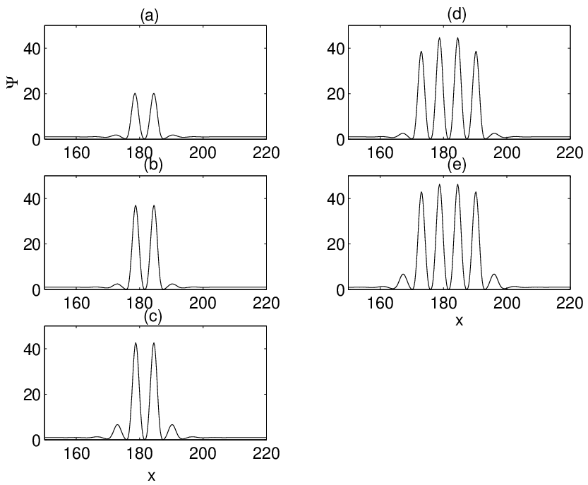
Using a shooting method (see Appendix) where the spatial coordinate is used as a dynamical variable in the stationary version of Eq. (11), we have found a self-localized solution. Taking it as an initial guess we have computed its branch by continuation techniques using a Newton method. Figure 4 shows the bifurcation diagram of localized states with an even number of peaks for . Another analogous curve for localized states with odd number of peaks (not shown) also exists. The curve shows a characteristic snaking structure. The branch follows a series of saddle-node bifurcations that transform unstable solutions into stable localized states, adding each time a peak at each side of the structure as one moves up. Typical localized states, indicated by bold dots in the inset of Figure 4, are presented in Figure 5. Solutions (b) and (d) in figure 5 are stable, while the rest are unstable. As can be seen from the inset in Figure 4, the region of existence of stable self-localized states is very narrow due to the proximity to the codimension-2 point. This region becomes larger as one moves away from this point in the direction of increasing the subcriticality of the pattern, i.e. increasing . However we can not go much further into that region, because the minimum of the population distribution approaches the trivial zero solution too much, and our simulations diverge. In this case further analysis is not possible and saturating terms should probably be included in Eq. (4) in order to observe stable localized states in wider parameter regions. We are unable to determine if the difficulties are only of numerical origin or if there is some more fundamental change of behavior or bifurcation when increasing subcriticality, perhaps associated to some spatial analog of the paradox of enrichment [38]. Further investigation is needed to clarify this point.
The localized solutions found (Fig. 5) consist on a few lumps of species, of a very high population density, which locally deplete close niche positions but do not make them completely empty. Further apart the effect of the lumps becomes unimportant and the density in the rest of the system consists on the stable homogeneous coexistence of species given by the homogeneous solution . The spacing between the lumps forming the localized patch is of the order of the periodicity of the extended pattern (Fig. 2). These regions can be then considered as portions of the periodic pattern embedded inside the stable homogeneous solution. To illustrate the stability of the self-localized states (b) and (d) in Fig. 5, we show in Figure 6 the switching dynamics of localized states starting from suitable initial conditions. The stability of the states has also been checked with respect to small additive noise.

V Localized states in the full nonlocal model
Once the precise conditions for the observation of subcritical patterns and localized structures have been determined for Eq. (11), we can discuss the implications for the kernel in the full nonlocal model (4). The main assumption is that we can apply to (4) the results of the previous section by using the values , , etc. arising from the expansion of the nonlocal kernel.
The necessary conditions for the existence of self-localized states were (for ) the subcriticality criterion (26), , and the instability condition (25), . In addition, the subcritical region increases with increasing , but as commented above our numerical results were unable to probe large values of without divergences. Figure (4) illustrate the situation for one of the largest values of attainable, , for which localized solutions appear for .
But it happens that this range of values of is far from what is achievable with an interaction kernel of competitive nature exclusively (i.e. one taking only positive values). To see this we note that a positively-defined and normalized () kernel can be interpreted as a probability density, so that and are its moments (see Eq. (6)): , . If , then . Applying the moment monotonicity inequality: , where , and using and , we have , or . This limiting value is well below the ones needed to observe self-localized solutions of Eq. (11) without encountering divergences. We can not completely discard in a rigorous manner the possibility of stable localized structures to exist for the nonlocal model at sufficiently large values of , nor the presence or other localized solution branches not captured within the differential approximation. But the fact is that we have been unable to find numerically self-localized solutions of (4) when using a purely competitive (i.e. positive) kernel .
A natural way to achieve the larger values of needed is to allow the kernel to take negative values close to or for large values of . This means the presence of facilitative interactions (mutualism, symbiosis, …) together with the competitive ones. We note that such combination of positive and negative interactions at different length scales was already proposed from biological reasoning in an early paper [29], an it is an important ingredient in the modeling of vegetation patterns [39]. Here we consider an integral kernel of the form:
| (27) |
were can take negative values modelling cooperative or facilitative interactions.
To find localized states in the full nonlocal model we perform then a continuation of the localized states from the differential to the integral kernel. The main difference between these two cases consists in the behavior of for : in the differential case, , while for the integral case , as illustrated in Fig. (1). Since the stability range of localized states is so small it is a challenge to find the parameters of the nonlocal kernel that support stable localized states. We show now, however, that at least for the lowest unstable localized state marked by a dashed red line in Figure (4) our continuation strategy is able to find them. To do so, we consider a linear combination of the integral kernel and the differential approximation in the truncated model (11) in the form:
| (28) |
where is a parameter characterizing how differential or how integral the resulting kernel is. So, for , the kernel is purely differential, while for , the kernel is purely integral.

We choose the parameters in such a way that the Fourier transform of is very close to the one of used in Fig. 4, except for high values of [see Figure 7(b)]. This implies that in real space the kernel takes negative values close to [ Figure 7(a)] . Now, using a continuation method we follow the self-localized solution from the differential case to the integral case . The corresponding modification of the kernel (28) and of the profile of the localized separatrix solution is shown in Fig. 7(c). In such a way we demonstrate the existence of localized states in the original model (4) for kernels fulfilling appropriate conditions.
VI Conclusions
By studying a differential truncation of the nonlocal Kolmogorov-Fisher model we have rigorously calculated the conditions by which periodic patterns are subcritical and we have demonstrated numerically the existence of the stable localized states in the differential approximation. These are patches of finite extent containing a number of lumps of species and arise on top of the homogeneous distribution. In contrast to other works, our results show that the necessary ingredient to observe stable self-localized states, namely the presence of subcritical patterns, is already present in systems with spatial coupling in the quadratic nonlinearity only, rather than nonlinearities of different orders being necessary. In consequence, the localized patches appear on a background of homogeneously distributed species coexistence, instead than on top of the no-species empty state. Extending the results obtained for the truncation to the full nonlocal model we find, however, that competitive interactions alone can not lead to the conditions for the observation of localized states, and facilitative interactions at or with distant locations in niche space, modeled by negative values of the kernel, are needed to observe this phenomenon.
From a biological point of view, the self-localization indicates that species with no particular advantage may predominate to competitors. A patch of species can be formed at any position of niche space by a particular initial condition or temporary perturbation. One should note that inhomogeneities in could increase or decrease the stability of the considered states. Although the results have been obtained in one dimensional space, and there are important differences with higher dimensional cases, we expect that the conditions for the observation of localized states will be qualitatively similar.
We acknowledge financial support from FEDER and MINECO (Spain) through grant FIS2012-30634 INTENSE@COSYP, and from Comunitat Autónoma de les Illes Balears. DG acknowledges support from CSIC (Spain) through grant number 201050I016.
Appendix: Numerical methods
To find the self-localized solution of (11) we write first the steady state condition :
| (29) |
introducing auxiliary quantities equation (29) is transformed to the system of ordinary differential equations:
| (30) |
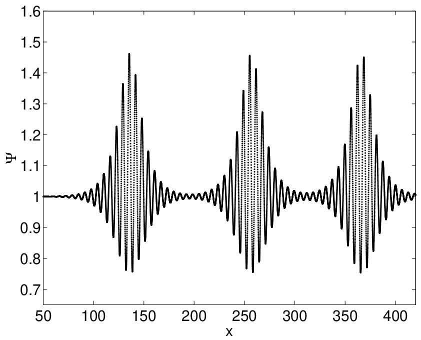
Interpreting now as a dynamical variable we solve the system (30) with initial conditions , , , and plus small perturbations. For parameters close to the subcritical bifurcation, trajectories showing localized pulses as the ones shown in Figure 8 are easily found. Taking one of the chirped pulses of this figure as a initial guess we can compute the branch shown in Fig. 4 using a Newton method and continuation techniques [40].
References
- [1] R. Holt, Theor. Popul. Biol. 12, 197 (1977).
- [2] P. Abrams, Ann. Rev. Ecol. Syst. 14, 359 (1983).
- [3] J. Murray, Mathematical Biology (Springer, Berlin, 1993).
- [4] J. Roughgarden, Theory of Population Genetics and Evolutionary Ecology: An Introduction (Macmillan Publishers, New York, 1979).
- [5] O. Leimar, A. Sasaki, M. Doebeli, and U. Dieckmann, J. Theor. Biol. 339, 3 (2013).
- [6] G. Barabás, S. Pigolotti, M. Gyllenberg, U. Dieckmann, and G. Meszéna, Evol. Ecol. Res. 14, 361 (2012).
- [7] M. Scheffer and E. H. van Nes, Proc. Natl. Acad. Sci. USA 103, 6230 (2006).
- [8] S. Pigolotti, C. López, and E. Hernández-García, Phys. Rev. Lett. 98, 258101 (2007).
- [9] E. Hernández-García, C. López, S. Pigolotti, and K. Andersen, Philosophical Transactions of the Royal Society A 367, 3183 (2009).
- [10] H. Fort, M. Scheffer, and E. van Nes, Theoretical Ecology 2, 171 (2009).
- [11] S. Pigolotti, C. Lopez, E. Hernandez-Garcia, and K. H. Andersen, Theoretical Ecology 3, 89 (2010).
- [12] E. Hernández-García and C. López, Phys. Rev. E 70, 016216 (2004).
- [13] C. López and E. Hernández-García, Physica D 199, 223 (2004).
- [14] M. Doebeli, H. Blok, O. Leimar, and U. Dieckmann, Proc. Royal Soc. B- Biol. Sci. 274, 347 (2007).
- [15] O. Leimar, M. Doebeli, and U. Dieckmann, Evolution 62, 807 (2008).
- [16] P. D. Woods and A. R. Champneys, Physica D 129, 147 (1999), ISSN 0167-2789.
- [17] P. Coullet, C. Riera, and C. Tresser, Phys. Rev. Lett. 84, 3069 (2000).
- [18] M. A. Fuentes, M. N. Kuperman, and V. M. Kenkre, Phys. Rev. Lett. 91, 158104 (2003).
- [19] Y. E. Maruvka and N. M. Shnerb, Phys. Rev. E 73, 011903 (2006).
- [20] E. M. Baptestini, M. A. de Aguiar, D. I. Bolnick, and M. S. Araújo, Journal of Theoretical Biology 259, 5 (2009).
- [21] M. G. Clerc, D. Escaff, and V. M. Kenkre, Phys. Rev. E 72, 056217 (2005).
- [22] M. G. Clerc, D. Escaff, and V. M. Kenkre, Phys. Rev. E 82, 036210 (2010).
- [23] O. Descalzi, M. Clerc, S. Residori, and G. Assanto, Localized States in Physics: Solitons and Patterns (Springer-Verlag, Berlin, Heidelberg, 2011).
- [24] N. Akhmediev and A. Ankiewicz, Dissipative Solitons: From Optics to Biology and Medicine (Springer-Verlag, Berlin Heidelberg, 2008).
- [25] A. Jacobo, D. Gomila, M.A. Matías, and P. Colet, Phys. Rev. A 78, 053821 (2008).
- [26] D. Escaff, Int. J. Bif. Chaos 19, 3509 (2009).
- [27] J. Burke and E. Knobloch, Phys. Rev. E 73, 056211 (2006).
- [28] D. Lawson and H. Jensen, Bulletin of Mathematical Biology 70, 1065 (2008).
- [29] N. Britton, Journal of Theoretical Biology 136, 57 (1989).
- [30] A. Sasaki, Journal of Theoretical Biology 186, 415 (1997), ISSN 0022-5193.
- [31] S. Genieys, V. Volpert, and P. Auger, Math. Model. Nat. Phenom. 1, 63 (2006).
- [32] B. Perthame and S. Génieys, Math. Model. Nat. Phenom. 2, 135 (2007).
- [33] G. Barabás, R. D’Andrea, G. Meszéna, and A. Ostling, Oikos 122, 1565 (2013).
- [34] S. Bochner, Duke Mathematical Journal 3, 726 (1937).
- [35] M. Fuentes, M. Kuperman, and V. Kenkre, J. Phys. Chem. B 108, 10505 (2004).
- [36] P. Becherer, A. N. Morozov, and W. van Saarloos, Physica D 238, 1827 (2009).
- [37] P. Manneville, Dissipative structures and weak turbulence (Academic Press Inc., San Diego, 1990).
- [38] M. L. Rosenzweig, Science 171, 385 (1971).
- [39] F. Borgogno, P. D’Odorico, F. Laio, and L. Ridolfi, Reviews of Geophysics 47, 136 (2009).
- [40] W. Press, S. Teukolsky, W. Vetterling, and B. Flannery, Numerical Recipes. The art of scientific computing (Cambridge University Press, New York, 2007).