Sparse Regularization: Convergence Of Iterative Jumping Thresholding Algorithm

Jinshan Zeng Shaobo Lin^∗ and Zongben Xu ^†^†thanks: J.S. Zeng is with the School of Computer and Information Engineering, Jiangxi Normal University, Nanchang 330022, and Beijing Center for Mathematics and Information Interdisciplinary Sciences (BCMIIS), Beijing, 100048, China. S.B. Lin is with the College of Mathematics and Information Science, Wenzhou University, Wenzhou 325035, Z.B. Xu is with the School of Mathematics and Statistics, Xi’an Jiaotong University, Xi’an 710049, P R China. (email: jsh.zeng@gmail.com, sblin1983@gmail.com, zbxu@mail.xjtu.edu.cn). $*$ Corresponding author: Shaobo Lin (sblin1983@gmail.com).

Abstract

In recent studies on sparse modeling, non-convex penalties have received considerable attentions due to their superiorities on sparsity-inducing over the convex counterparts. Compared with the convex optimization approaches, however, the non-convex approaches have more challenging convergence analysis. In this paper, we study the convergence of a non-convex iterative thresholding algorithm for solving sparse recovery problems with a certain class of non-convex penalties, whose corresponding thresholding functions are discontinuous with jump discontinuities. Therefore, we call the algorithm the iterative jumping thresholding (IJT) algorithm. The finite support and sign convergence of IJT algorithm is firstly verified via taking advantage of such jump discontinuity. Together with the assumption of the introduced restricted Kurdyka-Łojasiewicz (rKL) property, then the strong convergence of IJT algorithm can be proved. Furthermore, we can show that IJT algorithm converges to a local minimizer at an asymptotically linear rate under some additional conditions. Moreover, we derive a posteriori computable error estimate, which can be used to design practical terminal rules for the algorithm. It should be pointed out that the $l_{q}$ quasi-norm ( $0<q<1$ ) is an important subclass of the class of non-convex penalties studied in this paper. In particular, when applied to the $l_{q}$ regularization, IJT algorithm can converge to a local minimizer with an asymptotically linear rate under certain concentration conditions. We provide also a set of simulations to support the correctness of theoretical assertions and compare the time efficiency of IJT algorithm for the $l_{q}$ regularization ( $q=1/2,2/3$ ) with other known typical algorithms like the iterative reweighted least squares (IRLS) algorithm and the iterative reweighted $l_{1}$ minimization (IRL1) algorithm.

Index Terms:

Sparse regularization, non-convex optimization, iterative thresholding algorithm,

l_{q}

regularization (

0<q<1

), Kurdyka-Łojasiewicz inequality

I Introduction

The sparse vector recovery problems emerging in many areas of scientific research and engineering practice have attracted considerable attention in recent years ([1]-[4]). Typical applications include regression [5], visual coding [6], signal processing [7], compressed sensing [1], [2], machine learning [8], and microwave imaging [9]. These problems can be modeled as the following $l_{0}$ -norm regularized optimization problem

\min_{x\in\mathbf{R}^{N}}\left\{F(x)+\lambda\|x\|_{0}\right\},

(1)

where $F:\mathbf{R}^{N}\rightarrow[0,\infty)$ is a proper lower-semicontinuous function, $\|x\|_{0}$ , commonly called the $l_{0}$ -norm, denotes the number of nonzero components of $x$ and $\lambda>0$ is a regularization parameter. The $l_{0}$ regularized least squares problem is a special case of (1) where $F(x)=\frac{1}{2}\|Ax-y\|_{2}^{2}$ . Blumensath and Davies [10] proposed the iterative hard thresholding algorithm to solve this problem, and showed that the algorithm converges to a local minimizer. Recently, Lu and Zhang [11] proposed a penalty decomposition method for solving a more general class of $l_{0}$ regularized problems. In addition, Lu [12] proposed an iterative hard thresholding method and its variant for solving $l_{0}$ regularization over a conic constraint, and established its convergence as well as the iteration complexity.

Besides the $l_{0}$ regularized optimization problem, a more general class of problems are considered a lot in both practice and theory, that is,

\min_{x\in\mathbf{R}^{N}}\{F(x)+\lambda\Phi(x)\},

(2)

where $\Phi(x)$ is a certain separable, continuous penalty with $\Phi(x)=\sum_{i=1}^{N}\phi(|x_{i}|)$ , and $x=(x_{1},\cdots,x_{N})^{T}$ . One of the most important cases is the $l_{1}$ -norm with $\Phi(x)=\|x\|_{1}=\sum_{i=1}^{N}|x_{i}|$ . The $l_{1}$ -norm is convex and thus, the corresponding $l_{1}$ -norm regularized optimization problem can be efficiently solved. Because of this, the $l_{1}$ -norm becomes popular and has been accepted as a very useful tool for the modeling of the sparsity problems. Nevertheless, the $l_{1}$ -norm may not induce adequate sparsity when applied to certain applications [13], [14], [15], [16]. Alternatively, many non-convex penalties were proposed as relaxations of the $l_{0}$ -norm. Some typical non-convex examples are the $l_{q}$ -norm ( $0<q<1$ ) [14], [15], [16], Smoothly Clipped Absolute Deviation (SCAD) [17], Minimax Concave Penalty (MCP) [18] and Log-Sum Penalty (LSP) [13]. Compared with the $l_{1}$ -norm, the non-convex penalties can usually induce better sparsity while the corresponding non-convex regularized optimization problems are generally more difficult to solve.

There are mainly four classes of algorithms to solve the non-convex regularized optimization problem (2). The first one is the half-quadratic (HQ) algorithm [19], [20]. HQ algorithms can be efficient when both subproblems are easy to solve (particularly, when both subproblems have closed-form solutions). The second class is the iterative reweighted algorithm including iterative reweighted least squares (IRLS) minimization [21], [22], [23] and iterative reweighted $l_{1}$ -minimization (IRL1) [13] algorithms. Recently, Lu [24] extended some existing iterative reweighted methods and then proposed new variants for the general $l_{q}$ ( $0<q<1$ ) regularized unconstrained minimization problems. Nevertheless, the iterative reweighted algorithms can be only efficient when the corresponding non-convex penalty can be well approximated via the quadratic function or the weighted $l_{1}$ -norm function. The third class is the difference of convex functions algorithm (DC programming) [25], which is also called Multi-Stage (MS) convex relaxation [26]. The DC programming considers a proper decomposition of the objective function. Hence, it can be only applied to those non-convex penalties that can be decomposed as a difference of convex functions. The last class is the iterative thresholding algorithm, which fits the framework of the forward-backward splitting algorithm [27] and the generalized gradient projection algorithm [28] when applied to a separable non-convex penalty. Intuitively, the iterative thresholding algorithm can be viewed as a procedure of Landweber iteration projected by a certain thresholding operator. Thus, the thresholding operator plays a key role in the iterative thresholding algorithm. For some special non-convex penalties such as SCAD, MCP, LSP and $l_{q}$ -norms with $q=1/2,2/3$ , the associated thresholding operators can be expressed analytically [16], [29], [30]. Compared to the other types of non-convex algorithms such as the HQ, IRLS, IRL1 and DC programming algorithms, the iterative thresholding algorithm is easy to implement and has almost the least computational complexity for large scale problems [9], [31]. Consequently, the iterative thresholding algorithm becomes popular.

One of the significant differences between the convex and non-convex algorithms is that the convergence analysis of a non-convex algorithm is in general tricky. Although the effectiveness of the iterative thresholding algorithms for the non-convex regularized optimization problems has been verified in many applications, except for the iterative hard [12] and half [32] thresholding algorithms, the convergence of most of these algorithms has not been thoroughly investigated. More specifically, there are still three mainly open questions.

1.

When does the algorithm converge? Under what conditions, the iterative thresholding algorithm converges strongly in the sense that the whole sequence generated, regardless of the initial point, is convergent.
2.

Where does the algorithm converge? Does the algorithm converge to a global minimizer or more practically, a local minimizer due to the non-convexity of the optimization problem?
3.

What is the convergence rate of the algorithm?

I-A Main Contribution

In this paper, we give the convergence analysis for the iterative jumping thresholding algorithm (called IJT algorithm henceforth) for solving a certain class of non-convex regularized optimization problems. One of the most significant features of such non-convex problems is that the corresponding thresholding functions are discontinuous with jump discontinuities (see Fig. 1). Moreover, the corresponding thresholding functions are not nonexpansive in general. Among these non-convex penalties, the well-known $l_{q}$ -norm with $0<q<1$ is one of the most typical cases. The main contribution can be summarized as follows.

(a)

We prove that the supports and signs of any sequence generated by IJT algorithm can converge within finite iterations. Such property brings a possible way to construct a new sequence in a special subspace such that the new sequence has the same convergence behavior of the original sequence generated by IJT algorithm.
(b)

Under a further assumption that the objective function satisfies the so-called restricted Kurdyka-Łojasiewicz (rKL) property (see Definition 2) at some limit point, the strong convergence of IJT algorithm can be assuredly guaranteed (see Theorem 1). The introduced rKL property is generally weaker than the well-known Kurdyka-Łojasiewicz property that is widely used to study the convergence of nonconvex algorithms.
(c)

Under certain second-order conditions, we demonstrate that IJT algorithm converges to a local minimizer at an asymptotically linear rate (see Theorems 2-4). Such asymptotically linear convergence speed means that when the iterative vector is sufficiently close to the convergent point, the rate of convergence of IJT algorithm is linear. This implies that given a good initial guess, IJT algorithm can converge very fast.
(d)

As a typical case, we apply the developed convergence results to the $l_{q}$ regularization ( $0<q<1$ ). When applied to the $l_{q}$ regularization, IJT algorithm can converge to a local minimizer at an asymptotically linear rate as long as the matrix satisfies a certain concentration property (see Theorem 5).
(e)

We also provide simulations to support the correctness of theoretical assertions and compare the convergence speed of IJT algorithm for the $l_{q}$ regularization problems ( $q=1/2,2/3$ ) with other known typical algorithms like the iterative reweighted least squares (IRLS) algorithm and the iterative reweighted $l_{1}$ minimization (IRL1) algorithm.

I-B Notations and Organization

We denote $\mathbf{R}$ and $\mathbf{N}$ as the real number and natural number sets, respectively. For any vector $x\in\mathbf{R}^{N}$ , $x_{i}$ is its $i$ -th component, and for a given index set $I\subset I_{N}\triangleq\{1,2,\cdots,N\}$ , $x_{I}$ represents its subvector containing all the components restricted to $I$ . $I^{c}$ represents the complementary set of $I$ , i.e., $I^{c}=I_{N}\setminus I.$ $\|x\|_{2}$ represents the Euclidean norm of a vector $x$ . $Supp(x)$ is the support set of $x$ , i.e., $Supp(x)=\{i:|x_{i}|>0,i=1,\cdots,N\}$ . For any matrix $A\in\mathbf{R}^{N\times N}$ , $\sigma_{i}(A)$ and $\sigma_{\min}(A)$ ( $\lambda_{i}(A)$ and $\lambda_{\min}(A)$ ) denote as the $i$ -th and minimal singular values (eigenvalues) of $A$ , respectively. Similar to the vector case, for a given index set $I$ , $A_{I}$ represents the submatrix of $A$ containing all the columns restricted to $I$ . For any $z\in\mathbf{R}$ , $sign(z)$ denotes its sign function, i.e.,

sign(z)=\left\{\begin{array}[c]{ll}1,&\mbox{for}\ z>0\\ 0,&\mbox{for}\ z=0\\ -1,&\mbox{for}\ z<0\\ \end{array}\right..

The remainder of this paper is organized as follows. In section II, we give the problem settings and then introduce IJT algorithm with some basic properties. In section III, we give the convergence analysis of IJT algorithm. In section IV, we apply the established theoretical analysis to the $l_{q}$ ( $0<q<1$ ) regularization. In section V, we discuss some related work. In section VI, we conduct the simulations to substantiate the theoretical results. We conclude this paper in section VII.

II Iterative Jumping Thresholding Algorithm

In this section, we first present the basic settings of the considered non-convex regularized optimization problems, then introduce IJT algorithm for these problems. In the end of this section, we briefly review some basic properties of IJT algorithm obtained in [28].

II-A Problem Settings

We consider the following composite optimization problem

\min_{x\in\mathbf{R}^{N}}\{T_{\lambda}(x)=F(x)+\lambda\Phi(x)\},

(3)

where $\Phi(x)$ is assumed to be separable with $\Phi(x)=\sum_{i=1}^{N}\phi(|x_{i}|)$ . Moreover, we make several assumptions on the problem (3).

Assumption 1.

$F:\mathbf{R}^{N}\rightarrow[0,\infty)$ is weakly lower-semicontinuous and differentiable with Lipschitz continuous gradient, i.e., it holds that

\|\nabla F(u)-\nabla F(v)\|_{2}\leq L\|u-v\|_{2},\ \ \forall u,v\in\mathbf{R}^{N},

where $L>0$ is the Lipschitz constant.

It should be noted that Assumption 1 is a general assumption for $F$ . Many formulations in machine learning satisfy Assumption 1. For example, the following least squares and logistic loss functions are two commonly used functions which satisfy Assumption 1:

F(x)=\frac{1}{2M}\|Ux-y\|_{2}^{2}\ \ or\ \ \frac{1}{M}\sum_{i=1}^{M}\log(1+\exp(-y_{i}u_{i}^{T}x)),

where $u_{i}\in\mathbf{R}^{N}$ for $i=1,2,\cdots,M$ , $U=[u_{1},\cdots,u_{M}]^{T}\in\mathbf{R}^{M\times N}$ is a data matrix and $y=(y_{1},\cdots,y_{M})^{T}\in\mathbf{R}^{M}$ is a target vector. Moreover, in both signal and image processing, $F$ is commonly taken as the least squares of the observation model, that is,

F(x)=\|Ax-y\|_{2}^{2},

where $y\in\mathbf{R}^{M}$ is an observation vector and $A\in\mathbf{R}^{M\times N}$ is an observation matrix. It can be easily verified that such $F$ also satisfies Assumption 1.

In the following, we give some basic assumptions on $\phi$ , most of which were considered in [28].

Assumption 2.

$\phi:[0,\infty)\rightarrow[0,\infty)$ is continuous and satisfies the following assumptions:

(a)

$\phi$ is non-decreasing with $\phi(0)=0$ and $\phi(z)\rightarrow\infty$ when $z\rightarrow\infty$ .
(b)

For each $b>0$ , there exists an $a>0$ such that $\phi(z)\geq az^{2}$ for $z\in[0,b]$ .
(c)

$\phi$ is differentiable on $(0,\infty)$ and the derivative $\phi^{\prime}$ is strictly convex with $\phi^{\prime}(z)\rightarrow\infty$ for $z\rightarrow 0$ and $\phi^{\prime}(z)/z\rightarrow 0$ for $z\rightarrow\infty$ .
(d)

$\phi$ has a continuous second derivative $\phi^{\prime\prime}$ on $(0,\infty)$ .

In Assumption 2, (a) and (b) are taken from Assumption 3.1 in [28], while (c) and (d) are adapted from Assumption 3.2 in [28]. It can be observed that Assumption 2(a) ensures the coercivity of $\phi$ , and thus the existence of the minimizer of the optimization problem (3). Assumption 2(b) guarantees the weakly sequential lower semi-continuity of $\phi$ in $\l^{2}$ , and Assumption 2(c) induces the sparsity of the penalty $\Phi$ . In practice, there are many non-convex functions satisfying Assumption 2. Two of the most typical subclasses are $\phi(z)=z^{q}$ and $\phi(z)=\log(1+z^{q})$ with $q\in(0,1)$ as shown in Fig. 1.

Refer to caption — Fig. 1: Typical penalty functions $\phi$ satisfying Assumption 2 and the corresponding thresholding functions. More specifically, we plot the figures of the penalty functions $\phi(|z|)=|z|^{1/2},|z|^{2/3},\log(1+|z|^{1/3})$ , and their corresponding thresholding functions. For comparison, we also plot the figures of two well-known cases, i.e., $l_{0}$ -norm with $\phi(|z|)=\textsl{1}_{|z|>0}$ as the indicator function of $|z|>0$ , $l_{1}$ -norm with $\phi(|z|)=|z|$ , and their corresponding thresholding functions. (a) Typical penalty functions. (b) Thresholding functions.

II-B IJT Algorithm

In order to describe IJT algorithm, we need to generalize the proximity operator from the convex case to a non-convex penalty $\Phi$ , that is,

Prox_{\mu,\lambda\Phi}(x)=\arg\min_{u\in\mathbf{R}^{N}}\left\{\frac{\|x-u\|_{2}^{2}}{2\mu}+\lambda\Phi(u)\right\},

(4)

where $\mu>0$ is a parameter. Since $\Phi$ is separable, computing $Prox_{\mu,\lambda\Phi}$ is reduced to solve a one-dimensional minimization problem, that is,

prox_{\mu,\lambda\phi}(z)=\arg\min_{v\in\mathbf{R}}\left\{\frac{|z-v|^{2}}{2\mu}+\lambda\phi(|v|)\right\}.

(5)

Therefore,

Prox_{\mu,\lambda\Phi}(x)=(prox_{\mu,\lambda\phi}(x_{1}),\cdots,prox_{\mu,\lambda\phi}(x_{N}))^{T}.

(6)

As shown by (5), the proximity operator is defined through an optimization problem, which is commonly hard for computing and analysis. In order to present a simpler form of the proximity operator for analysis, we show a preparatory lemma in the following.

Lemma 1.

(Lemma 3.10 in [28]) Assume that $\phi$ satisfies Assumption 2, then

(a)

for each $\mu>0$ , the function $\rho_{\mu}:z\mapsto z+\lambda\mu\phi^{\prime}(z)$ is well defined on $\mathbf{R}_{+}$ and, moreover, it is strictly convex and attains a minimum at $z_{\mu}>0$ ;
(b)

the function $\psi:z\mapsto 2(\phi(z)-z\phi^{\prime}(z))/z^{2}$ is strictly decreasing and one-to-one on $(0,\infty)\rightarrow(0,\infty)$ ;
(c)

for any $z>0$ , it holds that $\phi^{\prime\prime}(z)<-\psi(z)<0$ ;
(d)

for any $z>0$ , $\phi^{\prime\prime}(z)$ is negative and monotonically increasing.

With Lemma 1, $prox_{\mu,\lambda\phi}$ can be expressed as follows.

Lemma 2.

(Lemma 3.12 in [28]) Assume that $\phi$ satisfies Assumption 2, then $prox_{\mu,\lambda\phi}$ is well defined and can be specified as

prox_{\mu,\lambda\phi}(z)=\left\{\begin{array}[c]{ll}sign(z)\rho_{\mu}^{-1}(|z|),&\mbox{for}\ |z|\geq\tau_{\mu}\\ 0,&\mbox{for}\ |z|\leq\tau_{\mu}\end{array}\right.,

(7)

for any $z\in\mathbf{R}$ with

\tau_{\mu}=\rho_{\mu}(\eta_{\mu})

(8)

and

\eta_{\mu}=\psi^{-1}((\lambda\mu)^{-1}).

(9)

Moreover, the range of $prox_{\mu,\lambda\phi}$ is $\{0\}\cup[\eta_{\mu},\infty)$ .

It can be observed that the proximity operator is discontinuous with a jump discontinuity, which is one of the most significant features of such a class of non-convex penalties studied in this paper. Moreover, it can be easily checked that the proximity operator is not nonexpansive in general. Due to these, the convergence analysis of the corresponding non-convex algorithm gets challenging. (Some specific proximity operators are shown in Fig. 1(b).)

With the definition of the proximity operator, IJT algorithm can be proposed to solve the non-convex regularized optimization problem (3). Formally, the iterative form of IJT algorithm can be expressed as follows

x^{n+1}\in Prox_{\mu,\lambda\Phi}(x^{n}-\mu\nabla F(x^{n})),

(10)

where $\mu>0$ is a step size parameter. For simplicity, we define

G_{\mu,\lambda\Phi}(x)=Prox_{\mu,\lambda\Phi}(x-\mu\nabla F(x))

for any $x\in\mathbf{R}^{N}$ . Henceforth, we call $prox_{\mu,\lambda\phi}$ the jumping thresholding function.

Remark 1.

For some specific $l_{q}$ -norm (say, $q=1/2,2/3$ ), the proximity operator can be expressed analytically [16], [29] (as shown in Fig. 1(b)).

Remark 2.

Although the $l_{0}$ -norm does not satisfy Assumption 2, the hard thresholding function is also discontinuous with jump discontinuities. Due to such discontinuity of the hard thresholding function, we will discuss that the convergence of the hard algorithm can be easily developed according to a similar analysis of IJT algorithm in Section III.

II-C Some Basic Properties of IJT Algorithm

In this subsection, we briefly review some basic properties of IJT algorithm, which serve as the basis of the further analysis in the next sections. Some of these properties can be found in [28].

Property 1.

(Proposition 2.1 and Corollary 2.2 in [28]) Let $\{x^{n}\}$ be a sequence generated by IJT algorithm with a bounded initialization. Assume that $0<\mu<\frac{1}{L}$ , then it holds

(a)

$T_{\lambda}(x^{n+1})\leq T_{\lambda}(x^{n})-\frac{1}{2}(\frac{1}{\mu}-L)\|x^{n+1}-x^{n}\|_{2}^{2}$ , and there exists a positive constant $T_{\lambda}^{*}$ such that $T_{\lambda}(x^{n})\rightarrow T_{\lambda}^{*}$ as $n\rightarrow\infty$ ;
(b)

$\|x^{n+1}-x^{n}\|_{2}\rightarrow 0$ as $n\rightarrow\infty$ .

Property 1(a) is commonly called the sufficient decrease property, which is a basic property desired for a descent method. With Property 1, the subsequential convergence of IJT algorithm can be easily claimed as the following property.

Property 2.

(Proposition 2.3 in [28]). Let $\{x^{n}\}$ be a sequence generated by IJT algorithm with a bounded initialization. Suppose that $0<\mu<\frac{1}{L}$ , then

(a)

each minimizer of $T_{\lambda}$ is a fixed point of $G_{\lambda\mu,\Phi}$ ;
(b)

there exists a convergent subsequence of $\{x^{n}\}$ and the limit point is a fixed point of $G_{\lambda\mu,\Phi}$ .

Besides Properties 1 and 2, we can derive the following property directly from the definition of the proximity operator.

Property 3.

Let $x^{*}$ be a fixed point of $G_{\lambda\mu,\Phi}$ and $\{x^{n}\}$ be a sequence generated by IJT algorithm, then it holds

(a)

$|x^{*}_{i}|\geq\tau_{\mu}/\mu$ and $[\nabla F(x^{*})]_{i}+\lambda sign(x_{i}^{*})\phi^{\prime}(|x_{i}^{*}|)=0$ for any $i\in Supp(x^{*})$ , and $|[\nabla F(x^{*})]_{i}|\leq\tau_{\mu}/\mu$ for any $i\in Supp(x^{*})^{c}$ ;
(b)

$x_{i}^{n+1}+\lambda\mu sign(x_{i}^{n+1})\phi^{\prime}(|x_{i}^{n+1}|)=x_{i}^{n}-\mu[\nabla F(x^{n})]_{i}$ for any $i\in Supp(x^{n+1})$ and $|x_{i}^{n}-\mu[\nabla F(x^{n})]_{i}|\leq\tau_{\mu}$ for any $i\in Supp(x^{n+1})^{c}$ , $n\in\mathbf{N}$ ,

where $[\nabla F(x^{*})]_{i}$ and $[\nabla F(x^{n+1})]_{i}$ represent the $i$ -th component of $\nabla F(x^{*})$ and $\nabla F(x^{n+1})$ respectively.

Actually, Property 3(a) is a certain type of optimality conditions of the non-convex regularized optimization problem (3). Moreover, we call $x^{*}$ a stationary point of (3) if $x^{*}$ satisfies Property 3(a), and we denote $\Omega_{\mu}$ the stationary point for a given $\mu$ .

III Convergence Analysis

In the last section, it can be only claimed that any sequence $\{x^{n}\}$ generated by IJT algorithm subsequentially converges to a stationary point. In this section, we will answer the open questions concerning IJT algorithm presented in the introduction, i.e., when, where and how fast does the algorithm converge? More specifically, we first prove that IJT algorithm converges to a stationary point under the so-called restricted Kurdyka-Łojasiewicz (rKL) property (see Definition 2), and then show that the stationary point is also a local minimizer of the optimization problem with some additional assumptions, and further demonstrate that the convergence rate of IJT algorithm is asymptotically linear.

III-A Restricted Kurdyka-Łojasiewicz Property

Kurdyka-Łojasiewicz (KL) property has been widely used to prove the convergence of the nonconvex algorithms (see, [27] for an instance). Specifically, the KL property is the following.

Definition 1.

([27]) The function $f:\mathbf{R}^{N}\rightarrow\mathbf{R}\cup\{+\infty\}$ is said to have the Kurdyka-Łojasiewicz property at $x^{*}\in$ dom $\partial f$ if there exist $\eta\in(0,+\infty]$ , a neighborhood $U$ of $x^{*}$ and a continuous concave function $\varphi:[0,\eta)\rightarrow\mathbf{R}_{+}$ such that:

(i)

$\varphi(0)=0$ ;
(ii)

$\varphi$ is ${\cal{C}}^{1}$ on $(0,\eta)$ ;
(iii)

for all $s\in(0,\eta)$ , $\varphi^{\prime}(s)>0$ ;
(iv)

for all $x$ in $U\cap\{x:f(x^{*})<f(x)<f(x^{*})+\eta\}$ , the Kurdyka-Łojasiewicz inequality holds

$\varphi^{\prime}(f(x)-f(x^{*}))dist(0,\partial f(x))\geq 1.$ (11)

Proper lower semi-continuous functions which satisfy the Kurdyka-Łojasiewicz inequality at each point of dom $\partial f$ are called KL functions.

Roughly speaking, KL inequality means that the function considered is sharp up to a reparametrization at a neighborhood of some point. From Definition 1, we can observe that KL inequality is actually certain type of first-order condition, which implies that the gradient (subgradient or subdifferential) of the transformed function via a concave function $\varphi$ is sharp and far away from zero. Functions satisfying the KL inequality include real analytic functions, semialgebraic functions and locally strongly convex functions (more information can be referred to Sec. 2.2 in [38] and references therein).

If further the objective function $T_{\lambda}$ in (3) is a KL function and the so-called relative error condition holds for the sequence $\{x^{n}\}$ generated by IJT algorithm, then according to Theorem 5.1 in [27], the strong convergence of IJT algorithm can naturally hold. However, on one hand, the relative error condition may be violated for $\{x^{n}\}$ . Actually, as justified in the consequent Lemma 5, such relative error condition only holds for the support sequence of $\{x^{n}\}$ . On the other hand, as listed in Appendix A, we can construct a one-dimensional function that satisfies Assumptions 1 and 2, but is not a KL function. This motivates us to introduce the following so-called restricted Kurdyka-Łojasiewicz (rKL) property to derive the convergence of IJT algorithm. To describe the definition of rKL property conveniently, we define a projection mapping associated with an index set $I\subset\{1,2,\cdots,N\}$ , that is,

P_{I}:\mathbf{R}^{N}\rightarrow\mathbf{R}^{K},P_{I}x=x_{I},\forall x\in\mathbf{R}^{N}.

We also denote $P_{I}^{T}$ as the transpose of $P_{I}$ , i.e.,

P_{I}^{T}:\mathbf{R}^{|I|}\rightarrow\mathbf{R}^{N},(P_{I}^{T}z)_{I}=z\ \text{and}\ (P_{I}^{T}z)_{I^{c}}=0,\forall z\in\mathbf{R}^{|I|},

where $|I|$ is the cardinality of $I$ and $I^{c}=\{1,2,\cdots,N\}\setminus I$ .

Definition 2.

A function $f:\mathbf{R}^{N}\rightarrow\mathbf{R}\cup\{+\infty\}$ is said to have the $I$ -restricted Kurdyka-Łojasiewicz property at $x^{*}\in$ dom $\partial f$ with $I$ being a given subset of $\{1,2,\cdots,N\}$ , if the function $g:\mathbf{R}^{|I|}\rightarrow\mathbf{R}\cup\{+\infty\},g(z)=f(P_{I}^{T}z)$ satisfies the KL inequality at $z^{*}=x_{I}^{*}.$

Obviously, the introduced rKL property is weaker than the KL property. If $I=\{1,2,\cdots,N\}$ , then rKL property is exactly equivalent to the KL property. From Definition 2, rKL property only requires the subdifferential of the function with respect to a part of variables can get sharp after certain a concave transform, while KL property requires such well property for all the variables around some point. It can be observed that rKL property is a natural extension of KL property. Assume that $f_{1}:\mathbf{R}^{n_{1}}\rightarrow\mathbf{R}$ is a KL function, and $f_{2}:\mathbf{R}^{n_{2}}\rightarrow\mathbf{R}$ is an arbitrary function. Let $f:\mathbf{R}^{n_{1}+n_{2}}\rightarrow\mathbf{R},f(u)=f_{1}(u_{I_{n_{1}}})+f_{2}(u_{I_{n_{1}}^{c}})$ , where $I_{n_{1}}=\{1,\cdots,n_{1}\}$ and $I_{n_{1}}^{c}=\{n_{1}+1,\cdots,n_{1}+n_{2}\}$ . Then obviously, $f$ is a $I_{n_{1}}$ -rKL function, but not a KL function. In the following, we will give a sufficient condition of the rKL property.

Lemma 3.

Given an index set $I\subset\{1,2,\cdots,N\}$ , consider the function $g(z)=f(P_{I}^{T}z)$ . Assume that $z^{*}$ is a stationary point of $g$ , and $g$ is twice continuously differentiable at a neighborhood of $z^{*}$ , i.e., $B(z^{*},\epsilon_{0})$ . Moreover, if $\nabla^{2}g(z^{*})$ is nonsingular, then $f$ satisfies $I$ -rKL property at the point $P_{I}^{T}z^{*}$ . Actually, it holds

|g(z)-g(z^{*})|\leq C^{*}\|\nabla g(z)\|_{2}^{2},\forall z\in B(z^{*},\epsilon),

for some $0<\epsilon<\epsilon_{0}$ and a positive constant $C^{*}>0$ .

The proof of this lemma is shown in Appendix B. From Lemma 3, $g$ actually satisfies the KL inequality at $z^{*}$ with a desingularizing function of the form $\varphi(s)=c\sqrt{s},$ where $c>0$ is a constant. Distinguished with the well-known KL inequality condition, the sufficient condition listed in the above lemma is some type of second-order condition, i.e., the Hessian of $g$ is nonsingular at some stationary point $z^{*}$ . The similar condition is also used to guarantee the convergence of the steepest descent method in [39] (Theorem 2, pp. 266). Obviously, if a stationary point $z^{*}$ is a strictly local minimizer (or maximizer), or a strict saddle point of $g$ , then the nonsingularity of $\nabla^{2}g(z^{*})$ holds naturally.

III-B Convergence To A Stationary Point

As analyzed in the section II, we have known that the sequence $\{x^{n}\}$ converges weakly. Let $\cal{X}$ be the limit point set of $\{x^{n}\}$ , $I^{n}=Supp(x^{n})$ . In the following, we first show that both the support and sign of the sequence will converge within finite iterations, and also any limit point $x^{*}\in\cal{X}$ has the same support and sign. These results are stated as the following lemma.

Lemma 4.

Let $\{x^{n}\}$ be a sequence generated by IJT algorithm. Assume that $0<\mu<\frac{1}{L}$ , then there exist a sufficiently large positive integer $n^{*}$ , an index set $I$ and a sign vector $S^{*}$ such that when $n>n^{*}$ , it holds

(a)

$I^{n}=I$ ;
(b)

$Supp(x^{*})=I,\forall x^{*}\in\cal{X}$ ;
(c)

$sign(x^{n})=S^{*}$ ;
(d)

$sign(x^{*})=S^{*},\forall x^{*}\in\cal{X}$ .

The proof of this lemma is presented in Appendix C. This lemma gives a possible way to construct a new sequence on a special subspace that has the same convergence behavior of $\{x^{n}\}$ . Thus, if we can prove the convergence of the new sequence, then the strong convergence of $\{x^{n}\}$ can naturally be claimed. Specifically, such new sequence can be constructed as follows. By Lemma 4, there exists a sufficiently large integer $n^{*}>0$ such that when $n>n^{*}$ ,

I^{n}=I\ \text{and}\ sign(x^{n})=sign(x^{*}).

Therefore, we can claim that $\{x^{n}\}$ converges to $x^{*}$ if the new sequence $\{x^{i+n^{*}}\}_{i\in\mathbf{N}}$ converges to $x^{*}$ , which is also equivalent to the convergence of the sequence $\{z^{i+n^{*}}\}_{i\in\mathbf{N}}$ , i.e.,

z^{i+n^{*}}\rightarrow z^{*}\ \text{as}\ i\rightarrow\infty

(12)

with $z^{i+n^{*}}=P_{I}x^{i+n^{*}}$ and $z^{*}=P_{I}x^{*}$ . Let $\hat{z}^{n}=z^{n+n^{*}}$ , then $\{\hat{z}^{n}\}$ has the same convergence behavior of $\{x^{n}\}$ .

For any $\epsilon>0$ , we define a one-dimensional real space

\mathbf{R}_{\epsilon}=\mathbf{R}\setminus(-\epsilon,\epsilon).

Particularly, let $\mathbf{R}_{0}=\mathbf{R}\setminus\{0\}$ . Denote ${\cal{Z}}^{*}=P_{I}{\cal{X}}=\{P_{I}x^{*}:x^{*}\in{\cal{X}}\}$ . We define two new functions $T:\mathbf{R}_{\eta_{\mu}/2}^{K}\rightarrow\mathbf{R}$ and $f:\mathbf{R}_{\eta_{\mu}/2}^{K}\rightarrow\mathbf{R}$ with

T(z)=T_{\lambda}(P_{I}^{T}z)\text{\ and\ }f(z)=F(P_{I}^{T}z),

(13)

for any $z\in\mathbf{R}_{\eta/2}^{K}$ , respectively. For any $z^{*}\in{\cal{Z}}^{*}$ , it can be observed that $z^{*}\in\mathbf{R}_{\eta_{\mu}}^{K}$ by Lemma 2, and $z^{*}$ is indeed a critical point of $T$ from Property 3(a). Moreover, we define a series of mappings $\phi_{1,m}:\mathbf{R}_{0}^{m}\rightarrow\mathbf{R}^{m}$ and $\phi_{2,m}:\mathbf{R}_{0}^{m}\rightarrow\mathbf{R}^{m\times m}$ as follows

\displaystyle\phi_{1,m}(z)=(sign(z_{1})\phi^{\prime}(|z_{1}|),\cdots,sign(z_{m})\phi^{\prime}(|z_{m}|))^{T},

(14)

\displaystyle\phi_{2,m}(z)=diag(\phi^{\prime\prime}(|z_{1}|),\cdots,\phi^{\prime\prime}(|z_{m}|)),

(15)

$m=1,\cdots,N$ , where $diag(z)$ represents the diagonal matrix generated by $z$ . For brevity, we will denote $\phi_{1,m}$ and $\phi_{2,m}$ as $\phi_{1}$ and $\phi_{2}$ respectively when $m$ is fixed and there is no confusion.

By Properties 1-3, we can easily justify that $\{\hat{z}^{n}\}$ satisfies the following so-called sufficient decrease, relative error and continuity conditions.

Lemma 5.

$\{\hat{z}^{n}\}$ satisfies the following conditions:

(a)

(Sufficient decrease condition). For each $n\in\mathbf{N}$ ,

$T(\hat{z}^{n+1})\leq T(\hat{z}^{n})-\frac{1}{2}(\frac{1}{\mu}-L)\|\hat{z}^{n+1}-\hat{z}^{n}\|_{2}^{2}.$
(b)

(Relative error condition). For each $n\in\mathbf{N}$ ,

$\|\nabla T(\hat{z}^{n+1})\|_{2}\leq(\frac{1}{\mu}+L)\|\hat{z}^{n+1}-\hat{z}^{n}\|_{2}.$
(c)

(Continuity condition). There exists a subsequence $\{\hat{z}^{n_{j}}\}_{j\in\mathbf{N}}$ and $z^{*}$ such that

$\hat{z}^{n_{j}}\rightarrow z^{*}\ \text{and}\ T(\hat{z}^{n_{j}})\rightarrow T(z^{*}),\ \text{as}\ j\rightarrow\infty.$

From this lemma, if $T$ further has the KL property at the limit point $z^{*}$ , then according to Theorem 2.9 in [27], $\{\hat{z}^{n}\}$ definitely converges to $z^{*}$ . Lemma 5(a) and (c) are obvious by Properties 1-2, the specific form of $T$ and the construction of $\{\hat{z}^{n}\}$ . Lemma 5(b) holds mainly due to Property 3(b) and Assumptions 1-2. Specifically, by Property 3(b), it can be easily checked that

\displaystyle\hat{z}^{n+1}+\lambda\mu\phi_{1}(\hat{z}^{n+1})=\hat{z}^{n}-\mu\nabla f(\hat{z}^{n}),

which implies

		$\displaystyle\mu(\nabla f(\hat{z}^{n+1})+\lambda\phi_{1}(\hat{z}^{n+1}))=$
		$\displaystyle(\hat{z}^{n}-\hat{z}^{n+1})+\mu(\nabla f(\hat{z}^{n+1})-\nabla f(\hat{z}^{n})).$

Thus,

\displaystyle\|\nabla T(\hat{z}^{n+1})\|_{2}=\frac{1}{\mu}\|(\hat{z}^{n}-\hat{z}^{n+1})+\mu(\nabla f(\hat{z}^{n+1})-\nabla f(\hat{z}^{n}))\|_{2}.

By Assumption 1, $\nabla F$ is Lipschitz continuous with the Lipschitz constant $L$ , then

		$\displaystyle\\|\nabla f(\hat{z}^{n+1})-\nabla f(\hat{z}^{n})\\|_{2}$
		$\displaystyle=\\|[\nabla F(P_{I}^{T}\hat{z}^{n+1})]_{I}-[\nabla F(P_{I}^{T}\hat{z}^{n})]_{I}\\|_{2}$
		$\displaystyle\leq\\|\nabla F(P_{I}^{T}\hat{z}^{n+1})-\nabla F(P_{I}^{T}\hat{z}^{n})\\|_{2}$
		$\displaystyle\leq L\\|P_{I}^{T}\hat{z}^{n+1}-P_{I}^{T}\hat{z}^{n}\\|_{2}=L\\|\hat{z}^{n+1}-\hat{z}^{n}\\|_{2}.$

Therefore,

\|\nabla T(\hat{z}^{n+1})\|_{2}\leq(\frac{1}{\mu}+L)\|\hat{z}^{n+1}-\hat{z}^{n}\|_{2}.

By Lemma 5 and the construction form of $\{\hat{z}^{n}\}$ , we can obtain the following convergence result of IJT algorithm.

Theorem 1.

Assume that $F$ and $\phi$ satisfy Assumptions 1 and 2, respectively. Consider any sequence $\{x^{n}\}$ generated by IJT algorithm with a bounded initialization. Suppose that $0<\mu<\frac{1}{L}$ , then $\{x^{n}\}$ converges subsequentially to a set $\cal{X}$ . If further $T_{\lambda}$ satisfies the $I$ -rKL property at some limit point $x^{*}\in{\cal{X}}$ with $I=Supp(x^{*})$ , then the whole sequence $\{x^{n}\}$ indeed converges to $x^{*}$ .

The first part of this theorem states that the sequence $\{x^{n}\}$ converges subsequentially to a limit point set $\cal{X}$ as long as the step size parameter $\mu$ is sufficiently small. The second part shows that the objective function further satisfies the introduced rKL property at some limit point $x^{*}$ , then the sequence $\{x^{n}\}$ converges to $x^{*}$ .

Furthermore, combining Lemma 3 and Theorem 1, we can obtain the following corollary.

Corollary 1.

Assume that $F$ and $\phi$ satisfy Assumptions 1 and 2, respectively. Consider any sequence $\{x^{n}\}$ generated by IJT algorithm with a bounded initialization. Suppose that $0<\mu<\frac{1}{L}$ , and if further there exists a limit point $x^{*}$ such that $F$ is twice continuously differentiable at $x^{*}$ and $\nabla^{2}T(P_{I}x^{*})$ is nonsingular, then the whole sequence $\{x^{n}\}$ indeed converges to $x^{*}$ .

III-C Convergence To A Local Minimizer

As shown in Corollary 1, if $\nabla^{2}T(P_{I}x^{*})$ is nonsingular at some limit point $x^{*}$ , then the sequence generated by IJT algorithm converges to $x^{*}$ , which is also a stationary point. In this subsection, we will justify that $x^{*}$ is also a local minimizer of the optimization problem if $\nabla^{2}T(P_{I}x^{*})$ is positive definite.

Theorem 2.

Suppose that $F$ and $\phi$ satisfy Assumptions 1 and 2, respectively. Assume that $0<\mu<\frac{1}{L}$ , and the sequence $\{x^{n}\}$ generated by IJT algorithm converges to $x^{*}$ . Then $x^{*}$ is a local minimizer of $T_{\lambda}$ provided that $F$ is twice continuously differentiable at $x^{*}$ and $\nabla^{2}T(P_{I}x^{*})$ is positive definite.

The proof of this theorem is rather intuitive. In the following, we will present some simple derivations. By Property 3(a) we have

[\nabla F(x^{*})]_{I}+\lambda\phi_{1}(x_{I}^{*})=0.

(16)

This together with the condition of the theorem

\nabla^{2}T(P_{I}x^{*})=\nabla_{II}^{2}F(x^{*})+\lambda\phi_{2}(x_{I}^{*})\succ 0

imply that the second-order optimality conditions hold at $x^{*}=(x_{I}^{*},0)$ , where $\nabla_{II}^{2}F(x^{*})={\frac{\partial^{2}F(x)}{\partial x_{I}^{2}}}{\big|}_{x=x^{*}}.$ For sufficiently small vector $h$ , we denote $x_{h}^{*}=(x_{I}^{*}+h_{I},0)$ . It then follows

F(x_{h}^{*})+\lambda\sum_{i\in I}\phi(|x_{i}^{*}+h_{i}|)\geq F(x^{*})+\lambda\sum_{i\in I}\phi(|x_{i}^{*}|).

(17)

Furthermore, by Assumption 2(c), it obviously holds that

\phi(t)>(\|[\nabla F(x^{*})]_{I^{c}}\|_{\infty}+2)t/\lambda,

for sufficiently small $t>0$ . By this fact and the differentiability of $F$ , one can observe that for sufficiently small $h$ , there hold

		$\displaystyle F(x^{}+h)-F(x_{h}^{})+\lambda\sum_{i\in I^{c}}\phi(\|h_{i}\|)$
		$\displaystyle=h_{I^{c}}^{T}[\nabla F(x^{*})]_{I^{c}}+\lambda\sum_{i\in I^{c}}\phi(\|h_{i}\|)+o(h_{I^{c}})$
		$\displaystyle\geq\sum_{i\in I^{c}}(\\|[\nabla F(x^{})]_{I^{c}}\\|_{\infty}-[\nabla F(x^{})]_{i}+1)\|h_{i}\|\geq 0.$		(18)

Summing up the above two inequalities (17)-(18), one has that for all sufficiently small $h$ ,

T_{\lambda}(x^{*}+h)-T_{\lambda}(x^{*})\geq 0,

(19)

and hence $x^{*}$ is a local minimizer.

Actually, we can observe that when $h\neq 0$ , then at least one of these two inequalities (17) and (18) will hold strictly, which implies that $x^{*}$ is a strictly local minimizer.

III-D Asymptotically Linear Convergence Rate

In order to derive the rate of convergence of IJT algorithm, we first show some observations on $\nabla F$ and $\phi^{\prime}$ in the neighborhood of $x^{*}$ . For any $0<\varepsilon<\eta_{\mu}$ , we define a neighborhood of $x^{*}$ as follows

{\cal{N}}(x^{*},\varepsilon)=\{x\in\mathbf{R}^{N}:\|x_{I}-x_{I}^{*}\|_{2}<\varepsilon,x_{I^{c}}=0\}.

If $F$ is twice continuously differentiable at $x^{*}$ and also $\lambda_{\min}(\nabla_{II}^{2}F(x^{*}))>0$ , then for any $x\in{\cal{N}}(x^{*},\varepsilon)$ , there exist two sufficiently small positive constants $c_{F}$ and $c_{\phi}$ (both $c_{F}$ and $c_{\phi}$ depending on $\varepsilon$ with $c_{F}\rightarrow 0$ and $c_{\phi}\rightarrow 0$ as $\varepsilon\rightarrow 0$ ) such that

		$\displaystyle\langle[\nabla F(x)]_{I}-[\nabla F(x^{})]_{I},x_{I}-x_{I}^{}\rangle$		(20)
		$\displaystyle\geq(\lambda_{\min}(\nabla_{II}^{2}F(x^{}))-c_{F})\\|x_{I}-x_{I}^{}\\|_{2}^{2},$

and

		$\displaystyle\langle\phi_{1}(x_{I})-\phi_{1}(x_{I}^{}),x_{I}-x_{I}^{}\rangle$		(21)
		$\displaystyle\geq(\phi^{\prime\prime}(e)-c_{\phi})\\|x_{I}-x_{I}^{*}\\|_{2}^{2},$

where (21) holds for $\phi^{\prime}$ being strictly convex on $(0,\infty)$ , and thus $\phi^{\prime\prime}$ being nondecreasing on $(0,\infty)$ , consequently, $\min_{i\in I}\phi^{\prime\prime}(|x_{i}^{*}|)=\phi^{\prime\prime}(\min_{i\in I}|x_{i}^{*}|)$ . With the observations (20) and (21), we obtain the following theorem.

Theorem 3.

Suppose that $F$ and $\phi$ satisfy Assumptions 1 and 2, respectively. Assume that the sequence $\{x^{n}\}$ generated by IJT algorithm converges to $x^{*}$ . Let $e=\min_{i\in I}|x_{i}^{*}|$ . Moreover, if $F$ is twice continuously differentiable at $x^{*}$ and the following conditions hold

(a)

$\lambda_{\min}(\nabla_{II}^{2}F(x^{*}))>0$ ;
(b)

$0<\lambda<-\frac{\lambda_{\min}(\nabla_{II}^{2}F(x^{*}))}{\phi^{\prime\prime}(e)},$
(c)

$0<\mu<\min\{\frac{2(\lambda_{\min}(\nabla_{II}^{2}F(x^{*}))+\lambda\phi^{\prime\prime}(e))}{L^{2}-(\lambda\phi^{\prime\prime}(e))^{2}},\frac{1}{L}\}$ ,

then there exists a sufficiently large positive integer $n_{0}$ and a constant $\rho^{\ast}\in(0,1)$ such that when $n>n_{0},$

\|x^{n+1}-x^{\ast}\|_{2}\leq\rho^{\ast}\|x^{n}-x^{\ast}\|_{2},

and

\|x^{n+1}-x^{*}\|_{2}\leq\frac{\rho^{*}}{1-\rho^{*}}\|x^{n+1}-x^{n}\|_{2}.

The proof of Theorem 3 is presented in Appendix D. This theorem states that IJT algorithm has asymptotically linear convergence rate under certain conditions. Let $z^{*}=P_{I}x^{*}$ . Conditions (a) and (b) in this theorem imply that the Hessian of $T$ at $z^{*}$ , $\nabla^{2}T(z^{*})$ is strongly positive definite, since $\lambda_{\min}(\nabla^{2}T(z^{*}))=\lambda_{\min}(\nabla^{2}f(z^{*})+\lambda\phi_{2}(z^{*}))\geq\lambda_{\min}(\nabla^{2}f(z^{*}))+\lambda\cdot\lambda_{\min}(\phi_{2}(z^{*}))=\lambda_{\min}(\nabla^{2}f(z^{*}))+\lambda\phi^{\prime\prime}(e)>0.$ Thus, $T$ is locally strongly convex at $z^{*}$ . Theorem 3 actually implies that the auxiliary sequence $\{\hat{z}^{n}\}$ converges linearly if $T$ is strongly convex at $z^{*}$ and the step size parameter $\mu$ is sufficiently small. As shown by this theorem, if we can fortunately obtain a sufficiently good initialization, then IJT algorithm may converge fast with a linear rate. On the other hand, Theorem 3 also provides a posteriori computable error estimation of the algorithm, which can be used to design an efficient terminal rule of IJT algorithm.

It can be observed that the conditions of Theorem 3 are slightly stricter than those of Corollary 1, and thus, $x^{*}$ is also a local minimizer under the conditions of Theorem 3. In the following, we will show that the condition on $\mu$ in Theorem 3 can be extended to $0<\mu<1/L$ if we add some additional assumptions on the higher order differentiability of $\phi$ in the neighborhood of the local minimizer $x^{*}$ . We state this as the following theorem.

Theorem 4.

Assume that $0<\mu<\frac{1}{L}$ . Let $\{x^{n}\}$ be a sequence generated by IJT algorithm and converge to $x^{*}$ . Let $e=\min_{i\in I}|x_{i}^{*}|$ . Moreover, if $F$ is twice continuously differentiable at $x^{*}$ and the following conditions hold

(a)

$\lambda_{\min}(\nabla_{II}^{2}F(x^{*}))>0$ ,
(b)

$0<\lambda<-\frac{\lambda_{\min}(\nabla_{II}^{2}F(x^{*}))}{\phi^{\prime\prime}(e)},$
(c)

for any sufficiently small $0<\varepsilon<\eta_{\mu}$ , the derivative of $\phi^{\prime\prime}$ , $\phi^{\prime\prime\prime}$ is well-defined, bounded and nonzero on the set $\cup_{i\in I}B(x_{i}^{*},\varepsilon)$ , where $B(x_{i}^{*},\varepsilon):=(x_{i}^{*}-\varepsilon,x_{i}^{*}+\varepsilon)$ ,

then there exists a sufficiently large positive integer $n_{0}>0$ and a constant $\rho\in(0,1)$ such that when $n>n_{0},$

\|x^{n+1}-x^{\ast}\|_{2}\leq\rho\|x^{n}-x^{\ast}\|_{2},

and

\|x^{n+1}-x^{*}\|_{2}\leq\frac{\rho}{1-\rho}\|x^{n+1}-x^{n}\|_{2}.

The proof of this theorem is given in Appendix E. Note that the condition (c) can be easily satisfied if the penalty $\phi$ has the continuous third-order derivative on $(0,\infty)$ . In the next section, we will show that the $l_{q}$ -norm ( $0<q<1$ ) is one of the most typical subclass of these non-convex penalties that satisfy the condition (c) in Theorem 4.

IV Application to $l_{q}$ Regularization ( $0<q<1$ )

In this section, we apply the established theoretical results to a typical case, $l_{q}$ regularization with $0<q<1$ .

Mathematically, $l_{q}$ $(0<q<1)$ regularization can be formulated as follows

\min_{x\in\mathbf{R}^{N}}\left\{T_{\lambda}(x)=\frac{1}{2}\|Ax-y\|_{2}^{2}+\lambda\|x\|_{q}^{q}\right\},

where $A\in\mathbf{R}^{M\times N}$ (commonly, $M<N$ ) is usually called the sensing matrix, $y\in\mathbf{R}^{M}$ is called the measurement vector, $x$ is commonly assumed to be sparse, i.e., $\|x\|_{0}\ll N$ , and $\|x\|_{q}^{q}=\sum_{i=1}^{N}|x_{i}|^{q}$ . Thus, in such special case, $F(x)=\frac{1}{2}\|Ax-y\|_{2}^{2}$ and $\Phi(x)=\|x\|_{q}^{q}$ with $\phi(x)=x^{q}$ defined on $(0,\infty)$ . In [28], Bredies and Lorenz demonstrated that the one-dimensional proximity operator $prox_{\mu,\lambda|\cdot|^{q}}$ of $l_{q}$ -norm can be expressed as

prox_{\mu,\lambda|\cdot|^{q}}(z)=\left\{\begin{array}[c]{ll}(\cdot+\lambda\mu qsign(\cdot)|\cdot|^{q-1})^{-1}(z),&|z|\geq\tau_{\mu,q}\\ 0,&|z|\leq\tau_{\mu,q}\end{array}\right.

(22)

for any $z\in\mathbf{R}$ with

\tau_{\mu,q}=\frac{2-q}{2-2q}(2\lambda\mu(1-q))^{\frac{1}{2-q}},

(23)

\eta_{\mu,q}=(2\lambda\mu(1-q))^{\frac{1}{2-q}},

(24)

and the range of $prox_{\mu,\lambda|\cdot|^{q}}$ is $\{0\}\cup[\eta_{\mu,q},\infty)$ . Furthermore, for some special $q$ (say, $q=1/2,2/3$ ), the corresponding proximity operators can be expressed analytically [16], [29].

According to [27] (See Example 5.4, page 122), the function $T_{\lambda}(x)=\frac{1}{2}\|Ax-y\|_{2}^{2}+\lambda\|x\|_{q}^{q}$ is a KL function and obviously satisfies the rKL propety at any limit point. By applying Theorem 1 to the $l_{q}$ regularization, we can obtain the following corollary directly.

Corollary 2.

Let $\{x^{n}\}$ be a sequence generated by IJT algorithm for $l_{q}$ regularization with $q\in(0,1)$ . Assume that $0<\mu<\frac{1}{\|A\|_{2}^{2}}$ , then $\{x^{n}\}$ converges to a stationary point of $l_{q}$ regularization.

In [27], Attouch et al. showed the convergence of the inexact forward-backward splitting algorithm for $l_{q}$ regularization (See Theorem 5.1, page 118) under exactly the same condition of Corollary 2 . Furthermore, it is easy to check that $F(x)=\frac{1}{2}\|Ax-y\|_{2}^{2}$ and $\phi(z)=z^{q}$ satisfy Assumptions 1 and 2, respectively. In addition, $\phi(z)=z^{q}$ also satisfies the condition (c) in Theorem 4 naturally. Therefore, as a direct corollary of Theorem 4, we show the asymptotically linear convergence rate of IJT algorithm for $l_{q}$ regularization as follows.

Corollary 3.

Assume that $0<\mu<\|A\|_{2}^{-2}$ . Let $\{x^{n}\}$ be a sequence generated by IJT algorithm for $l_{q}$ ( $0<q<1$ ) regularization and converge to $x^{*}$ . Let $I=Supp(x^{*})$ and $e=\min_{i\in I}|x_{i}^{*}|$ . Moreover, if the following conditions hold:

(a)

$\lambda_{\min}(A_{I}^{T}A_{I})>0$ ,
(b)

$0<\lambda<\frac{\lambda_{\min}(A_{I}^{T}A_{I})e^{2-q}}{q(1-q)},$

then there exists a sufficiently large positive integer $n_{0}$ and a constant $\rho\in(0,1)$ such that when $n>n_{0},$

\|x^{n+1}-x^{\ast}\|_{2}\leq\rho\|x^{n}-x^{\ast}\|_{2},

and

\|x^{n+1}-x^{*}\|_{2}\leq\frac{\rho}{1-\rho}\|x^{n+1}-x^{n}\|_{2}.

In addition, $x^{*}$ is also a local minimizer of $l_{q}$ regularization.

The condition (b) in Corollary 3 means that the regularization parameter should be sufficiently small to guarantee that the limit point is a local minimizer. Instead of adding the assumption on the regularization parameter $\lambda$ , we give another sufficient condition characterized by the matrix $A$ . Such condition is mainly derived via taking advantage of the specific form of the threshold value (24). More specifically, by (24), it holds

e\geq\eta_{\mu,q}=(2\lambda\mu(1-q))^{\frac{1}{2-q}}.

(25)

Then if $\frac{\lambda_{\min}(A_{I}^{T}A_{I})}{\|A\|_{2}^{2}}>\frac{q}{2}$ and

\frac{q}{2\lambda_{\min}(A_{I}^{T}A_{I})}<\mu<\frac{1}{\|A\|_{2}^{2}},

(26)

the conditions in Corollary 3 hold naturally. Therefore, we can obtain the following theorem on the asymptotically linear convergence rate of IJT algorithm applied to $l_{q}$ regularization.

Theorem 5.

(a)

$\frac{\lambda_{\min}(A_{I}^{T}A_{I})}{\|A\|_{2}^{2}}>\frac{q}{2}$ ,
(b)

$\frac{q}{2\lambda_{\min}(A_{I}^{T}A_{I})}<\mu<\frac{1}{\|A\|_{2}^{2}},$

then there exists a sufficiently large positive integer $n_{0}$ and a constant $\rho\in(0,1)$ such that when $n>n_{0},$

\|x^{n+1}-x^{\ast}\|_{2}\leq\rho\|x^{n}-x^{\ast}\|_{2},

and

\|x^{n+1}-x^{*}\|_{2}\leq\frac{\rho}{1-\rho}\|x^{n+1}-x^{n}\|_{2}.

In addition, $x^{*}$ is also a local minimizer of $l_{q}$ regularization.

From Theorem 5, it means that if the matrix $A$ satisfies a certain concentration property and the step size $\mu$ is chosen appropriately, then IJT algorithm can converge to a local minimizer at an asymptotically linear rate. Note that the condition (a) in Theorem 5 implies $\frac{q}{2\lambda_{\min}(A_{I}^{T}A_{I})}<\frac{1}{\|A\|_{2}^{2}}$ naturally. Thus, the condition (b) of Theorem 5 is a natural and reachable condition and, furthermore, whenever this condition is satisfied, the sequence $\{x^{n}\}$ is indeed convergent by Corollary 2. This shows that only the condition (a) is essential in Theorem 5. We notice that the condition (a) is a concentration condition on eigenvalues of the submatrix $A_{I}^{T}A_{I}$ , and, in particular, it implies

\lambda_{\min}(A_{I}^{T}A_{I})>q\lambda_{\max}(A_{I}^{T}A_{I})/2,

or equivalently

Cond(A_{I}^{T}A_{I}):=\frac{\lambda_{\max}(A_{I}^{T}A_{I})}{\lambda_{\min}(A_{I}^{T}A_{I})}<\frac{2}{q},

(27)

where $Cond(A_{I}^{T}A_{I})$ is the condition number of $A_{I}^{T}A_{I}$ . (27) thus shows that the submatrix $A_{I}^{T}A_{I}$ is well-conditioned with the condition number lower than $2/q$ .

In recent years, a property called the restricted isometry property (RIP) of a matrix $A$ was introduced to characterize the concentration degree of the eigenvalues of its submatrix with $k$ columns [45]. A matrix $A$ is said to be of the $k$ -order RIP (denoted then by $\delta_{k}$ -RIP) if there exists a $\delta_{k}\in(0,1)$ such that

(1-\delta_{k})\|x\|_{2}^{2}\leq\|Ax\|_{2}^{2}\leq(1+\delta_{k})\|x\|_{2}^{2},~\forall\|x\|_{0}\leq k.

(28)

In other words, the RIP ensures that all submatrices of $A$ with $k$ columns are close to an isometry, and therefore distance-preserving. Let $K=\|x^{\ast}\|_{0}$ . It can be seen from (28) that if $A$ possesses $\delta_{K}$ -RIP with $\delta_{K}<\frac{2-q}{2+q}$ , then

Cond(A_{I}^{T}A_{I})\leq\frac{1+\delta_{K}}{1-\delta_{K}}<\frac{2}{q}.

Thus, we can claim that when $A$ satisfies a certain RIP, the condition (a) in Theorem 5 can be satisfied. In particular, we have the following proposition.

Proposition 1.

Assume that $K<N/2$ and $A$ satisfies $\delta_{K}$ -RIP with $\delta_{K}<\frac{2-q}{2+2qN/K}$ or $\delta_{2K}$ -RIP with $\delta_{2K}<\frac{2-q}{2+qN/K}$ , then the condition (a) in Theorem 5 holds.

This can be directly checked by the facts that $\lambda_{\min}(A_{I}^{T}A_{I})\geq 1-\delta_{K}$ , $\lambda_{\min}(A_{I}^{T}A_{I})\geq 1-\delta_{2K}$ , $\lambda_{\max}(A^{T}A)\leq 1+\delta_{N}$ , $\delta_{N}\leq\frac{2N}{K}\delta_{K}$ and $\delta_{N}\leq\frac{N}{K}\delta_{2K}$ (c.f. Proposition 1 in [46]).

From Proposition 1, we can see, for instance, when $q=1/2,K/N=1/3$ and $A$ satisfies $\delta_{K}$ -RIP with $\delta_{K}<3/10$ or $\delta_{2K}$ -RIP with $\delta_{2K}<3/7$ , the condition (a) in Theorem 5 is satisfied, and therefore, by Theorem 5, IJT algorithm converges to a local minimizer of the $l_{q}$ regularization at an asymptotically linear rate. It is noted that in the condition of Proposition 1, we always have $\delta_{k}<\frac{2-q}{2+4q}$ and $\delta_{2k}<\frac{2-q}{2+2q}.$

Remark 3.

In a recent paper [32], Zeng et al. have justified the convergence of a specific iterative thresholding algorithm called the iterative half thresholding algorithm for $l_{1/2}$ regularization. It can be observed that the convergence results of the iterative half thresholding algorithm obtained in [32] is just a special case of the results presented in this section.

Remark 4.

Recently, Lu [12] proposed an iterative hard thresholding method and its variant for solving $l_{0}$ regularization over a conic constraint, and established its convergence as well as the iteration complexity. Although the $l_{0}$ -norm does not satisfies Assumption 2, it can be observed that the finite support and sign convergence property (i.e., Lemma 4) holds naturally for hard algorithm due to the hard thresholding function possesses the similar discontinuity of the jumping thresholding function. Furthermore, once the support of the sequence converges, the iterative form of hard algorithm is equal to the simple Landweber iteration, and thus the convergence and asymptotically linear convergence rate of hard algorithm can be directly claimed.

V Related Work

Recently, Attouch et al. [27] have justified the convergence of a family of descent methods by assuming the objective function has the KL property [36], [37], and also the generated sequence satisfies the sufficient decrease property, relative error condition and continuity condition (Sec. 2.3 in [27]). Instead of the well-known KL inequality condition, we introduce a weaker condition called the rKL property to check the convergence of IJT algorithm. Besides the strong convergence, we also justify the asymptotically linear convergence rate of IJT algorithm under certain second-order conditions. Compared with the other algorithms including HQ [35], FOCUSS [21], IRL1 [42] and DC programming [25] algorithms, we derive a sufficient condition instead of the direct assumption that the accumulation points are isolated, for the convergence of IJT algorithm. Furthermore, the convergence speed of IJT algorihtm is also demonstrated in this paper.

Besides the aforementioned non-convex algorithms, there are some other related algorithms. In the following, we will compare the obtained theoretical results of IJT algorithm with those of these algorithms. The first class of closely related algorithms are the iterative shrinkage and thresholding (IST) algorithms, which mainly refer to two generic algorithms and some specific algorithms. The first generic algorithm related to IJT algorithm is the generalized gradient projection (called GGP for short) algorithm [33], [28]. In [33], the GGP algorithm was proposed for the $l_{1}$ regularization problem. In such a convex setting, the finite support convergence and eventually linear convergence rate was given in [33]. In [28], Bredies and Lorenz extended the GGP algorithm to solve the following general non-convex optimization model in the infinite-dimensional Hilbert space

\min_{x\in\mathbf{X}}\left\{F(x)+\lambda\Phi(x)\right\},

(29)

where $\mathbf{X}$ is an infinite-dimensional Hilbert space, $F:\mathbf{X}\rightarrow[0,\infty)$ is assumed to be a proper lower-semicontinuous function with Lipschitz continuous gradient $\nabla F(x)$ , and $\Phi:\mathbf{X}\rightarrow[0,\infty)$ is weakly lower-semicontinuous (possibly non-smooth and non-convex). Furthermore, the iterative form of the GGP algorithm is specified as

x^{n+1}\in Prox_{\mu,\lambda\Phi}(x^{n}-\mu\nabla F(x^{n})),

where $Prox_{\mu,\lambda\Phi}$ represents the proximity operator of $\Phi$ as defined in (4). It can be observed that IJT algorithm is a special case of GGP algorithm when applied to a separable $\Phi$ in the finite-dimensional real space. Nevertheless, it was only justified that GGP algorithm can converge subsequentially to a stationary point [28] (that is, there is a subsequence that converges to a stationary point). However, as a specific case of GGP algorithm, we have justified that IJT algorithm can assuredly converge to a local minimizer at an asymptotically linear convergence rate under certain conditions.

Another closely related generic algorithm is the general iterative shrinkage and thresholding (GIST) algorithm suggested in [30]. The GIST algorithm is proposed for the following general non-convex regularized optimization problem

\min_{x\in\mathbf{R}^{N}}\{F(x)+\lambda R(x)\},

(30)

where $F$ is assumed to be continuously differentiable with Lipschitz continuous derivative, and $R(x)$ is a continuous function and can be rewritten as the difference of two different convex functions. As compared with Assumption 2, we can find that the optimization model considered in this paper is distinguished from the model (30) studied in [30]. Moreover, only the subsequential convergence of the GIST algorithm can be justified in [30], while the convergence of the whole sequence and further the asymptotically linear convergence rate of IJT algorithm are demonstrated in this paper.

Besides these two generic algorithms, there are some other specific iterative thresholding algorithms related to IJT algorithm. Among them, the hard algorithm and the soft algorithm are two representatives, which respectively solves the $l_{0}$ regularization and $l_{1}$ regularization [10], [40]. It was demonstrated in [10], [40] that when $\mu=1$ both $hard$ and $soft$ algorithms can converge to a stationary point whenever $\|A\|_{2}<1$ . These classical convergence results can be generalized when a step size parameter $\mu$ is incorporated with the IST procedures, and in this case, the convergence condition becomes

0<\mu<\|A\|_{2}^{-2}.

(31)

It can be seen from Corollary 2 that (31) is the exact condition of the convergence of IJT algorithm when applied to the $l_{q}$ regularization with $0<q<1$ , which then supports that the classical convergence results of IST has been extended to the non-convex $l_{q}$ ( $0<q<1$ ) regularization case. Furthermore, it was shown in [41] that when the measurement matrix $A$ satisfies the so-called finite basis injective (FBI) property and the stationary point possesses a strict sparsity pattern, the soft algorithm can converge to a global minimizer of $l_{1}$ regularization with a linear convergence rate. Such result is not surprising because of the convexity of $l_{1}$ regularization. As for convergence speed of the hard algorithm, it was demonstrated in [10] that under the condition $\mu=1$ and $\|A\|_{2}<1$ , hard algorithm will converge to a local minimizer with an asymptotically linear convergence rate. However, as algorithms for solving non-convex models, Corollary 3 and Theorem 5 reveal that IJT algorithm shares the same asymptotic convergence speed with hard algorithm.

VI Numerical Experiments

We conduct a set of numerical experiments in this section to substantiate the validity of the theoretical analysis on the convergence of IJT algorithm. While the effectiveness of IJT algorithm applied to large-scale applications such as the synthetic aperture radar (SAR) imaging and image processing can be referred to [9] and [29]. (The corresponding matlab code of IJT algorithm can be referred to https://github.com/JinshanZeng/IJT_Alg.)

VI-A Convergence Rate Justification

We start with an experiment to confirm the linear rate of asymptotic convergence. For this purpose, given a sparse signal $x$ with dimension $N=500$ and sparsity $k=15,$ shown as in Fig. 2(b), we considered the signal recovery problem through observation $y=Ax,$ where the measurement matrix $A$ is of dimension $M\times N=250\times 500$ with Gaussian $\mathcal{N}(0,1/250)$ i.i.d. entries. Such measurement matrix is known to satisfy (with high probability) the RIP with optimal bounds [43], [44]. We then applied IJT algorithm to the problem with two different non-convex penalties, that is, $\phi(|z|)=|z|^{1/2},|z|^{2/3}$ . In both cases, the jumping thresholding operators can be analytically expressed as shown in [16] and [29], respectively, and thus the corresponding IJT algorithms can be efficiently implemented. In both cases, we took $\lambda=0.001$ and $\mu=0.99\|A\|_{2}^{-2}$ . Moreover, we considered two different initial guesses including 0 and the solution of the $l_{1}$ -minimization problem to justify the effect on the convergence speed. The experiment results are reported in Fig. 2.

It can be seen from Fig. 2(a) how the iteration error ( $\|x^{(n)}-x^{\ast}\|_{2})$ varies. More specifically, when 0 was taken as the initial guess, after approximately $1300$ and $1700$ iterations, IJT algorithm converges to a stationary point with a linear decay rate for both penalties $\phi(|z|)=|z|^{1/2}$ and $\phi(|z|)=|z|^{2/3}$ , as shown by the blue and black lines in Fig. 2(a), respectively. While from the red and green lines in Fig. 2(a), if we took the solution of the $l_{1}$ -minimization problem as the initialization, the IJT algorithm converges to a stationary point with a linear convergence rate starting from almost the first iteration for both penalties. This indicates that the solution of the $l_{1}$ -minimization problem is a good initialization, which is sufficiently close to the stationary point. Moreover, Fig. 2(b) shows that the original sparse signal has been recovered by IJT algorithm with very high accuracy. This experiment clearly justifies the convergence properties of IJT algorithm we have verified, particularly the expected asymptotically linear convergence rate of IJT algorithm is substantiated.

VI-B On effect of $\mu$

As shown by the iterative form (10) of IJT algorithm, the step size parameter $\mu$ is a crucial parameter of IJT algorithm. In this subsection, we conducted a series of experiments to verify the effect of $\mu$ on both the recovery precision and convergence speed. The measurement matrix and the true sparse signal were set the same as in Subsection 6.1. We applied IJT algorithm for both $\phi(|z|)=|z|^{1/2}$ and $\phi(|z|)=|z|^{2/3}$ with different $\mu$ to recover the sparse signal from the given measurements. We varied $\mu$ uniformly in the interval $(0,\|A\|_{2}^{-2})$ for 100 times. The experimental results are shown in Fig. 3.

From Fig. 3(a), we can observe that $\mu$ has almost no effect on the recovery quality of IJT algorithm for both penalties. While the number of iterations required to attain the same terminal rule decreases monotonically as $\mu$ increasing as demonstrated by Fig. 3(b) and (c). This phenomenon coincides with the common sense. It demonstrates that when $\mu$ is larger, the algorithm converges faster, and thus fewer iterations are required to attain a given precision. More specifically, as shown by Fig. 3(b), the number of iterations decreases much sharper when $\mu<0.02$ . Accordingly, we recommend that in practical application of IJT algorithm, a larger step size $\mu$ should be taken. In addition, we found that the performance of IJT algorithm for $l_{1/2}$ regularization is slightly better than the performance for $l_{2/3}$ regularization in the perspectives of both recovery quality and iteration number, as shown in Fig. 3. The additional advantage of IJT algorithm for $l_{1/2}$ regularization in the perspective of cpu time was also demonstrated in the next subsection over IJT algorithm for $l_{2/3}$ regularization.

VI-C Comparisons with Reweighted Techniques

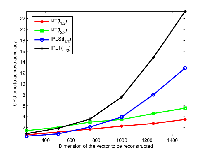
This set of experiments were conducted to compare the time costs of IJT algorithm, IRLS algorithm [23] and IRL1 algorithm [13] for solving the same signal recovery problem with different settings $\{k,M,N\},$ where, as in Subsection 8.2 in [23], we took $k=5$ , $N=\{250,500,750,1000,1250,1500\}$ and $M=N/5$ . We applied IJT algorithm for two different penalties, i.e., $\phi(|z|)=|z|^{1/2}$ and $\phi(|z|)=|z|^{2/3}$ . We implemented all algorithms using Matlab without any specific optimization. In particular, we used the CVX Matlab package by Michael Grant and Stephen Boyd (http://www.stanford.edu/ $\sim$ boyd/cvx/) to perform the weighted $l_{1}$ -minimization at each iteration step of IRL1 algorithm. Again, the measurement matrix $A$ was taken to be the $M\times N$ dimensional matrices with i.i.d. Gaussian $\mathcal{N}(0,\frac{1}{M})$ entries. The experiment results are shown in Fig. 4. As shown in Fig. 4(a), when $N$ is lower than $500$ , IRLS algorithm is slightly faster than IJT algorithm with $\phi(|z|)=|z|^{1/2}$ . This is due to that in the low-dimensional cases, the computational burden of solving a low-dimensional least squares problem in IRLS is relatively low. Nevertheless, when $N>500,$ it can be observed that IJT algorithm with $\phi(|z|)=|z|^{1/2}$ outperforms both IRLS and IRL1 algorithms in the perspective of CPU time. Furthermore, we can observe from Fig. 4(b) that as $N$ increases, the CPU times cost by IRL1 and IRLS algorithms increase much faster than IJT algorithm, that is to say, the outperformance of IJT algorithm in time cost can get more significant as dimension increases.

VII Conclusion

We have conducted a study of the convergence of IJT algorithm for a class of non-convex regularized optimization problems. One of the most significant features of such class of iterative thresholding algorithms is that the associated thresholding functions are discontinuous with jump discontinuities. Moreover, the corresponding thresholding functions are in general not nonexpansive due to the nonconvexity of the penalties. Among such class of non-convex optimization problems, the $l_{q}$ ( $0<q<1$ ) regularization problem is one of the most typical subclass.

The main contribution of this paper is the establishment of the convergence and rate-of-convergence results of IJT algorithm for a certain class of non-convex optimization problems. We first prove the finite support and sign convergence of IJT algorithm as long as $0<\mu<1/L,$ where $L$ is the Lipschitz constant of $\nabla F.$ Then we show the strong convergence of IJT algorithm under certain a rKL property. Furthermore, we demonstrate that IJT algorithm converges to a local minimizer at an asymptotically linear rate under certain second-order conditions. When applied to the $l_{q}$ regularization, IJT algorithm can converge to a local minimizer at an asymptotically linear rate as long as the matrix satisfies a certain concentration property. The obtained convergence results to a local minimizer generalize those known for the soft and hard algorithms. We have also provided a set of simulations to support the correctness of the established theoretical assertions. The efficiency of IJT algorithm is further compared through simulations with the known reweighted techniques, another type of typical non-convex regularization algorithms.

Appendix

VII-A A non-KL function

In the following, we give a specific one-dimensional function that satisfies Assumptions 1 and 2, but not a KL function. Given any function $\phi$ satisfying Assumption 2, let $g=f+\phi$ with $f$ being defined as follows

f(z)=\left\{\begin{array}[c]{ll}a_{1}(z-b_{1})^{2}+c_{1},&\mbox{for}\ z\leq 1/2\\ \exp\left(-\frac{1}{(z-1)^{2}}\right)-\phi(z)+C,&\mbox{for}\ 1/2<z<1\\ C-\phi(1),&\mbox{for}\ z=1\\ \exp\left(-\frac{1}{(z-1)^{2}}\right)-\phi(z)+C,&\mbox{for}\ 1<z<3/2\\ a_{2}(z-b_{2})^{2}+c_{1},&\mbox{for}\ z\geq 3/2\end{array}\right.,

(32)

where $e=exp(1)$ , $a_{1}=80e^{-4}-\frac{1}{2}\phi^{\prime\prime}(\frac{1}{2}),b_{1}=\frac{1}{2}+\frac{16e^{-4}+\phi^{\prime}(\frac{1}{2})}{160e^{-4}-\phi^{\prime\prime}(\frac{1}{2})},$ $a_{2}=80e^{-4}-\frac{1}{2}\phi^{\prime\prime}(3/2),b_{2}=\frac{3}{2}-\frac{16e^{-4}-\phi^{\prime}(\frac{3}{2})}{160e^{-4}-\phi^{\prime\prime}(\frac{3}{2})},$ $C=\phi(\frac{3}{2})+\max\left\{\phi(\frac{1}{2})+a_{1}(\frac{1}{2}-b_{1})^{2},\phi(\frac{3}{2})+a_{2}(\frac{3}{2}-b_{2})^{2}\right\}$ , $c_{1}=C+e^{-4}-\phi(\frac{1}{2})-a_{1}(\frac{1}{2}-b_{1})^{2},$ and $c_{2}=C+e^{-4}-\phi(\frac{3}{2})-a_{2}(\frac{3}{2}-b_{2})^{2}.$ Thus,

g(z)=\left\{\begin{array}[c]{ll}a_{1}(z-b_{1})^{2}+c_{1}+\phi(|z|),&\mbox{for}\ z\leq 1/2\\ \exp\left(-\frac{1}{(z-1)^{2}}\right)+C,&\mbox{for}\ 1/2<z<1\\ C,&\mbox{for}\ z=1\\ \exp\left(-\frac{1}{(z-1)^{2}}\right)+C,&\mbox{for}\ 1<z<3/2\\ a_{2}(z-b_{2})^{2}+c_{1}+\phi(z),&\mbox{for}\ z\geq 3/2\end{array}\right..

(33)

When $1/2<z<3/2$ , we define a function $h(z)$ as

h(z)=\left\{\begin{array}[c]{ll}\exp\left(-\frac{1}{(z-1)^{2}}\right),&\mbox{for}\ 1/2<z<1\\ 0,&\mbox{for}\ z=1\\ \exp\left(-\frac{1}{(z-1)^{2}}\right),&\mbox{for}\ 1<z<3/2\\ \end{array}\right..

It can be easily checked that $f$ satisfies Assumption 1 due to the function $h$ is ${\cal{C}}^{\infty}$ and $\phi$ is ${\cal{C}}^{2}$ in the interval $(1/2,3/2)$ . However, according to [36] (Sec. 1, page 1), it shows that $h$ fails to satisfy the KL inequality (11) at $z=1$ . Therefore, $g$ must be not a KL function. The figures of $f$ and $g$ are shown in Fig. 5 with $\phi(|z|)=|z|^{1/2}$ .

VII-B Proof of Lemma 3

Proof.

Note that $z^{*}$ is a stationary point of $g$ , i.e., $\nabla g(z^{*})=0$ , then

		$\displaystyle\|g(z)-g(z^{})\|=\|g(z)-g(z^{})-\nabla g(z^{})^{T}(z-z^{})\|$
		$\displaystyle\leq\int_{0}^{1}\\|\nabla g(z^{}+t(z-z^{}))-\nabla g(z^{})\\|_{2}\\|z-z^{}\\|_{2}dt.$		(34)

Since $g$ is twice continuously differentiable at $B(z^{*},\epsilon_{0})$ , then it obviously exists constants $L_{g}>0$ such that

\|\nabla g(z^{*}+t(z-z^{*}))-\nabla g(z^{*})\|_{2}\leq L_{g}t\|z-z^{*}\|_{2},

for any $z\in B(z^{*},\epsilon_{0})$ and $t\in(0,1)$ . Thus, it follows

|g(z)-g(z^{*})|\leq\frac{L_{g}}{2}\|z-z^{*}\|_{2}^{2},\forall z\in B(z^{*},\epsilon_{0}).

(35)

On the other hand, for any $z\in B(z^{*},\epsilon_{0})$ , there exists a $t_{0}\in(0,1)$ such that

	$\displaystyle\\|\nabla g(z)\\|_{2}=\\|\nabla g(z)-\nabla g(z^{*})\\|_{2}$		(36)
	$\displaystyle=\\|\nabla^{2}g(z^{}+t_{0}(z-z^{}))(z-z^{*})\\|_{2}.$

Since $\nabla^{2}g(z^{*})$ is nonsingular and by the continuity of $\nabla^{2}g(z)$ at $B(z^{*},\epsilon_{0})$ , then there exists $0<\epsilon<\epsilon_{0}$ such that for any $z\in B(z^{*},\epsilon),$

\sigma_{\min}(\nabla^{2}g(z^{*}+t_{0}(z-z^{*})))\geq\min_{z\in B(z^{*},\epsilon)}\sigma_{\min}(\nabla^{2}g(z))>0.

Denote $\sigma_{\epsilon,z^{*}}=\min_{z\in B(z^{*},\epsilon)}\sigma_{\min}(\nabla^{2}g(z)),$ then (36) becomes

\displaystyle\|\nabla g(z)\|_{2}\geq\sigma_{\epsilon,z^{*}}\|z-z^{*}\|_{2}.

(37)

Let $C^{*}=\frac{L_{g}}{2\sigma_{\epsilon,z^{*}}^{2}}.$ Combining (35) and (37), it implies

|g(z)-g(z^{*})|\leq C^{*}\|\nabla g(z)\|_{2}^{2}.

Thus, we complete the proof of the lemma.

∎

VII-C Proof of Lemma 4

Proof.

(i) By Property 1(b), there exists a sufficiently large positive integer $n_{0}$ such that $\|x^{n}-x^{n+1}\|_{2}<\eta_{\mu}$ when $n>n_{0}$ . We first show that

I^{n+1}=I^{n},\forall n>n_{0}

(38)

by contradiction. Assume this is not the case, that is, $I^{n_{1}+1}\neq I^{n_{1}}$ for some $n_{1}>n_{0}$ . Then it is easy to derive a contradiction through distinguishing the following two possible cases:

Case 1: $I^{n_{1}+1}\neq I^{n_{1}}$ and $(I^{n_{1}+1}\cap I^{n_{1}})\subset I^{n_{1}+1}.$ In this case, there exists an $i_{n_{1}}$ such that $i_{n_{1}}\in I^{n_{1}+1}\setminus I^{n_{1}}$ . By Lemma 2, it then implies

\|x^{n_{1}+1}-x^{n_{1}}\|_{2}\geq|x_{i_{n_{1}}}^{n_{1}+1}|\geq\min_{i\in I^{n_{1}+1}}|x_{i}^{n_{1}+1}|\geq\eta_{\mu},

which contradicts to $\|x^{n_{1}+1}-x^{n_{1}}\|_{2}<\eta_{\mu}.$

Case 2: $I^{n_{1}+1}\neq I^{n_{1}}$ and $(I^{n_{1}+1}\cap I^{n_{1}})=I^{n_{1}+1}.$ Under this circumstance, it is obvious that $I^{n_{1}+1}\subset I^{n_{1}}$ . Thus, there exists an $k_{n_{1}}$ such that $k_{n_{1}}\in I^{n_{1}}\setminus I^{n_{1}+1}$ . It then follows from Lemma 2 that

\|x^{n_{1}+1}-x^{n_{1}}\|_{2}\geq|x_{k_{n_{1}}}^{n_{1}}|\geq\min_{i\in I^{n_{1}}}|x_{i}^{n_{1}}|\geq\eta_{\mu},

and it contradicts to $\|x^{n_{1}+1}-x^{n_{1}}\|_{2}<\eta_{\mu}$ . Thus, (38) holds true. It also means that the support set sequence $\{I^{n}\}$ converges. We denote $I$ the limit of $I^{n}$ . Then for any $n>n_{0},$ $I^{n}=I$ .

(ii) For any limit point $x^{*}\in\cal{X}$ , there exits a subsequence $\{x^{n_{j}}\}$ converging to $x^{*}$ , i.e.,

x^{n_{j}}\rightarrow x^{*}\ \ \text{as}\ \ j\rightarrow\infty.

(39)

Thus, there exists a sufficiently large positive integer $j_{0}$ such that $n_{j_{0}}>n_{0}$ and $\|x^{n_{j}}-x^{*}\|_{2}<\eta_{\mu}$ when $j\geq j_{0}$ . Similar to the proof procedure (i), it can be also claimed that $I^{n_{j}}=Supp(x^{*})$ for any $j\geq j_{0}$ . On the other hand, by (38), $I^{n_{j}}=I$ . Thus, for any limit point $x^{*}$ , $Supp(x^{*})=I$ .

Taking $n^{*}=n_{j_{0}}$ , then by the above analysis, it is obvious that the claims (a) and (b) in Lemma 4 hold true.

(iii) As $I^{n}=I=Supp(x^{*})$ for any $n>n^{*}$ and $x^{*}\in{\cal{X}}$ , it suffices to show that $sign(x_{i}^{n+1})=sign(x_{i}^{n})$ and $sign(x_{i}^{n_{j}})=sign(x_{i}^{*})$ for any $i\in I$ , $j\geq j_{0}$ , $n>n^{*}$ . Similar to the first two parts of the proof, we will first check that $sign(x_{i}^{n+1})=sign(x_{i}^{n})$ , and then $sign(x_{i}^{n_{j}})=sign(x_{i}^{*})$ for any $i\in I$ by contradiction. We now prove $sign(x_{i}^{n+1})=sign(x_{i}^{n})$ for any $i\in I$ and $n>n^{*}$ . Assume this is not the case. Then there exists an $i^{\ast}\in I$ such that $sign(x_{i^{*}}^{n+1})\neq sign(x_{i^{*}}^{n})$ , and hence,

sign(x_{i^{*}}^{n+1})sign(x_{i^{*}}^{n})=-1.

From Lemma 2, it is easy to check

	$\displaystyle\\|x^{n+1}-x^{n}\\|_{2}$	$\displaystyle\geq\|x_{i^{\ast}}^{n+1}-x_{i^{\ast}}^{n}\|=\|x_{i^{\ast}}^{n+1}\|+\|x_{i^{\ast}}^{n}\|$
		$\displaystyle\geq\min_{i\in I}\{\|x_{i}^{n+1}\|+\|x_{i}^{n}\|\}\geq 2\eta_{\mu},$

which contradicts again to $\|x^{n+1}-x^{n}\|_{2}<\eta_{\mu}$ . This contradiction shows $sign(x^{n+1})=sign(x^{n})$ when $n>n^{*}$ . It follows that the sign sequence $\{sign(x^{n})\}$ is convergent. Let $S^{*}$ be the limit of the sign sequence $\{sign(x^{n})\}$ . Similarly, we can also show that $sign(x^{n_{j}})=sign(x^{*})$ whenever $j\geq j_{0}$ . Therefore, $sign(x^{n})=S^{*}=sign(x^{*})$ when $n>n^{*}$ and for any $x^{*}\in{\cal{X}}$ . This finishes the proof of Lemma 4. ∎

VII-D Proof of Theorem 3

Proof.

Let $C_{1}=1+\lambda\mu\phi^{\prime\prime}(e)$ and $C_{2}=\sqrt{1-2\mu\lambda_{\min}(\nabla_{II}^{2}F(x^{*}))+\mu^{2}L^{2}}.$ By the assumptions of Theorem 3, it is easy to check that

C_{1}>C_{2}>0.

Since both $c_{F}$ and $c_{\phi}$ approach to zero as $\varepsilon$ approaches zero, then we can take a sufficiently small $0<\varepsilon<\eta_{\mu}$ such that

0<c_{F}<\min\left\{\frac{(C_{1}-C_{2})(C_{1}+3C_{2})}{8\mu},\lambda_{\min}(\nabla_{II}^{2}F(x^{*}))\right\},

and

0<c_{\phi}<\frac{C_{1}-C_{2}}{2\lambda\mu}.

Furthermore, let

\alpha_{F,\varepsilon}=\lambda_{\min}(\nabla_{II}^{2}F(x^{*}))-c_{F}\ \text{and}\ \alpha_{\phi,\varepsilon}=-\phi^{\prime\prime}(e)+c_{\phi},

then under assumptions of Theorem 3, there hold $0<\alpha_{F,\varepsilon}<L$ and $\alpha_{\phi,\varepsilon}>0,$ and further

\displaystyle 1-\lambda\mu\alpha_{\phi,\varepsilon}=1+\lambda\mu\phi^{\prime\prime}(e)-\lambda\mu c_{\phi}>\frac{C_{1}+C_{2}}{2}>0,

(40)

\displaystyle 1-2\mu\alpha_{F,\varepsilon}+\mu^{2}L^{2}\geq 1-2\mu\alpha_{F,\varepsilon}+\mu^{2}\alpha_{F,\varepsilon}^{2}\geq 0,

(41)

		$\displaystyle 1-2\mu\alpha_{F,\varepsilon}+\mu^{2}L^{2}=C_{2}^{2}+2\mu c_{F}$		(42)
		$\displaystyle<C_{2}^{2}+\frac{(C_{1}-C_{2})(C_{1}+3C_{2})}{4}=\left(\frac{C_{1}+C_{2}}{2}\right)^{2}.$

Since $\{x^{n}\}$ converges to $x^{*}$ , then for any $0<\varepsilon<\eta_{\mu}$ , there exists a sufficiently large integer $n_{0}>n^{*}$ (where $n^{*}$ is specified as in Lemma 4) such that

\|x^{n}-x^{*}\|_{2}<\varepsilon

when $n>n_{0}$ . Let $I^{n}=Supp(x^{n})$ . By Lemma 4, it holds $I^{n}=I$ and $sign(x^{n})=sign(x^{*})$ when $n>n_{0}$ . Furthermore, by Property 3, for any $i\in I$ ,

x_{i}^{*}+\lambda\mu sign(|x_{i}^{*}|)\phi^{\prime}(|x_{i}^{*}|)=x_{i}^{*}-\mu[\nabla F(x^{*})]_{i},

and

x_{i}^{n+1}+\lambda\mu sign(|x_{i}^{n+1}|)\phi^{\prime}(|x_{i}^{n+1}|)=x_{i}^{n}-\mu[\nabla F(x^{n})]_{i},

when $n>n_{0}$ . Consequently,

		$\displaystyle(x_{I}^{n+1}-x_{I}^{})+\lambda\mu(\phi_{1}(x_{I}^{n+1})-\phi_{1}(x_{I}^{}))$
		$\displaystyle=(x_{I}^{n}-x_{I}^{})-\mu([\nabla F(x^{n})]_{I}-[\nabla F(x^{})]_{I}),$

and then

		$\displaystyle\\|x_{I}^{n+1}-x_{I}^{}\\|_{2}^{2}+\lambda\mu\langle\phi_{1}(x_{I}^{n+1})-\phi_{1}(x_{I}^{}),x_{I}^{n+1}-x_{I}^{*}\rangle=$
		$\displaystyle\langle x_{I}^{n+1}-x_{I}^{},(x_{I}^{n}-x_{I}^{})-\mu([\nabla F(x^{n})]_{I}-[\nabla F(x^{*})]_{I})\rangle.$		(43)

By (21), the left side of (43) satisfies

		$\displaystyle\\|x_{I}^{n+1}-x_{I}^{}\\|_{2}^{2}+\lambda\mu\langle\phi_{1}(x_{I}^{n+1})-\phi_{1}(x_{I}^{}),x_{I}^{n+1}-x_{I}^{*}\rangle$
		$\displaystyle\geq(1-\lambda\mu\alpha_{\phi,\varepsilon})\\|x_{I}^{n+1}-x_{I}^{*}\\|_{2}^{2},$

and the right side of (43) satisfies

		$\displaystyle\langle x_{I}^{n+1}-x_{I}^{},(x_{I}^{n}-x_{I}^{})-\mu([\nabla F(x^{n})]_{I}-[\nabla F(x^{*})]_{I})\rangle\leq$
		$\displaystyle\\|x_{I}^{n+1}-x_{I}^{}\\|_{2}\\|(x_{I}^{n}-x_{I}^{})-\mu([\nabla F(x^{n})]_{I}-[\nabla F(x^{*})]_{I})\\|_{2}.$

Without loss of generality, we assume that $\|x_{I}^{n+1}-x_{I}^{*}\|_{2}>0$ , otherwise, it demonstrates that IJT algorithm converges to $x^{*}$ in finite iterations. Thus, it becomes

		$\displaystyle(1-\lambda\mu\alpha_{\phi,\varepsilon})\\|x_{I}^{n+1}-x_{I}^{*}\\|_{2}$		(44)
		$\displaystyle\leq\\|(x_{I}^{n}-x_{I}^{})-\mu([\nabla F(x^{n})]_{I}-[\nabla F(x^{})]_{I})\\|_{2}.$

Furthermore, by (20), it follows

		$\displaystyle\\|(x_{I}^{n}-x_{I}^{})-\mu([\nabla F(x^{n})]_{I}-[\nabla F(x^{})]_{I})\\|_{2}^{2}$
		$\displaystyle=\\|x_{I}^{n}-x_{I}^{}\\|_{2}^{2}+\mu^{2}\\|[\nabla F(x^{n})]_{I}-[\nabla F(x^{})]_{I}\\|_{2}^{2}$
		$\displaystyle-2\mu\langle x_{I}^{n}-x_{I}^{},[\nabla F(x^{n})]_{I}-[\nabla F(x^{})]_{I}\rangle$
		$\displaystyle\leq(1-2\mu\alpha_{F,\varepsilon}+\mu^{2}L^{2})\\|x_{I}^{n}-x_{I}^{*}\\|_{2}^{2}.$		(45)

Combing (44) and (45), it implies

\displaystyle\|x_{I}^{n+1}-x_{I}^{*}\|_{2}\leq\frac{\sqrt{1-2\mu\alpha_{F,\varepsilon}+\mu^{2}L^{2}}}{1-\lambda\mu\alpha_{\phi,\varepsilon}}\|x_{I}^{n}-x_{I}^{*}\|_{2}.

Let

\rho^{*}=\frac{\sqrt{1-2\mu\alpha_{F,\varepsilon}+\mu^{2}L^{2}}}{1-\lambda\mu\alpha_{\phi,\varepsilon}}.

By (40)-(42), it is easy to check that

0<\rho^{*}<1.

Thus, when $n>n_{0}$

		$\displaystyle\\|x^{n+1}-x^{}\\|_{2}=\\|x_{I}^{n+1}-x_{I}^{}\\|_{2}$		(46)
		$\displaystyle\leq\rho^{}\\|x_{I}^{n}-x_{I}^{}\\|_{2}=\rho^{}\\|x^{n}-x^{}\\|_{2}.$

Consequently, the asymptotic convergence rate of IJT algorithm is linear.

Moreover, the posteriori error bound can be easily derived by the triangle inequality

\|x^{n}-x^{*}\|_{2}\leq\|x^{n+1}-x^{*}\|_{2}+\|x^{n+1}-x^{n}\|_{2}

and (46). Therefore, we have completed the proof of Theorem 3. ∎

VII-E Proof of Theorem 4

Proof.

Let

c_{1}=\frac{1-\mu\lambda_{min}(\nabla_{II}^{2}F(x^{*}))}{1+\lambda\mu\phi^{\prime\prime}(e)}.

(47)

By the assumptions of Theorem 4, it holds $0<c_{1}<1$ . For any $0<c<1$ , let

g(c)=\max_{i\in I}\max_{\{x_{i}:|x_{i}-x_{i}^{*}|<c\eta_{\mu}\}}\left\{\frac{\lambda\mu|\phi^{\prime\prime\prime}(|x_{i}|)|}{2|1+\lambda\mu\phi^{\prime\prime}(|x_{i}^{*}|)|}\right\},

(48)

and

c_{\epsilon}(c)=\frac{1-c_{1}-\epsilon}{g(c)\eta_{\mu}},

(49)

for some $0<\epsilon<1-c_{1}.$ Since $g(c)$ is non-decreasing with respective to $c$ , and thus $c_{\epsilon}(c)$ is non-increasing with respect to $c$ . Therefore, there exists a positive constant $c^{*}$ such that

0<c^{*}<1\ \text{and}\ c^{*}<c_{\epsilon}(c^{*}).

(50)

Since $\{x^{n}\}$ converges to $x^{*}$ , then there exists an $n^{**}>n^{*}$ (where $n^{*}$ is specified as in Lemma 4), when $n>n^{**}$ , it holds

\|x^{n}-x^{*}\|_{2}<c^{*}\eta_{\mu}.

By Lemma 4, when $n>n^{**}$ , it holds $I^{n}=I$ and $sign(x^{n})=sign(x^{*})$ , and thus $\|x^{n}-x^{*}\|_{2}=\|x_{I}^{n}-x_{I}^{*}\|_{2}$ . By Property 3, for any $i\in I$ ,

		$\displaystyle(x_{i}^{n}-x_{i}^{})-\mu([\nabla F(x^{n})]_{i}-[\nabla F(x^{})]_{i})$
		$\displaystyle=(x_{i}^{n+1}-x_{i}^{})+sign(x_{i}^{})\lambda\mu(\phi^{\prime}(\|x_{i}^{n+1}\|)-\phi^{\prime}(\|x_{i}^{*}\|)).$

By Taylor expansion, for any $i\in I$ , there exists an $\xi_{i}\in(0,1)$ , such that

		$\displaystyle\phi^{\prime}(\|x_{i}^{n+1}\|)-\phi^{\prime}(\|x_{i}^{*}\|)=$
		$\displaystyle sign(x_{i}^{})\phi^{\prime\prime}(\|x_{i}^{}\|)(x_{i}^{n+1}-x_{i}^{})+\frac{1}{2}\phi^{\prime\prime\prime}(\|x_{i}^{\xi}\|)(x_{i}^{n+1}-x_{i}^{})^{2},$

where $x_{i}^{\xi}=x_{i}^{*}+\xi_{i}(x_{i}^{n+1}-x_{i}^{*})$ . Let $h^{n}=x^{n}-x^{*}$ , then by the above two inequalities, it follows

\Lambda_{1}h_{I}^{n+1}+\Lambda_{2}(h_{I}^{n+1}\odot h_{I}^{n+1})=h_{I}^{n}-\mu([\nabla F(x^{n})]_{I}-[\nabla F(x^{*})]_{I}),

(51)

where $\odot$ denotes the Hadamard product or elementwise product, $\Lambda_{1}$ and $\Lambda_{2}$ are two different diagonal matrices with

		$\displaystyle\Lambda_{1}(i,i)=1+\lambda\mu\phi^{\prime\prime}(\|x_{i}^{*}\|),$		(52)
		$\displaystyle\Lambda_{2}(i,i)=\frac{1}{2}sign(x_{i}^{*})\lambda\mu\phi^{\prime\prime\prime}(x_{i}^{\xi}).$

Moreover, by the twice differentiability of $F$ at $x^{*}$ , we have

[\nabla F(x^{n})]_{I}-[\nabla F(x^{*})]_{I}=\nabla_{II}^{2}F(x^{*})h_{I}^{n}+o(\|h_{I}^{n}\|_{2}).

(53)

Plugging (53) into (51), it becomes

\Lambda_{1}h_{I}^{n+1}+\Lambda_{2}(h_{I}^{n+1}\odot h_{I}^{n+1})=(\mathbf{I}-\mu\nabla_{II}^{2}F(x^{*}))h_{I}^{n}+o(\|h_{I}^{n}\|_{2}),

where $\mathbf{I}$ denotes as the identity matrix with the size $|I|\times|I|$ with $|I|$ being the cardinality of the set $I$ . By the assumptions of Theorem 4, for any $i\in I$ ,

		$\displaystyle\Lambda_{1}(i,i)=1+\lambda\mu\phi^{\prime\prime}(\|x_{i}^{*}\|)$
		$\displaystyle\geq 1+\lambda\mu\phi^{\prime\prime}(e)>1-\mu\lambda_{\min}(\nabla^{2}_{II}F(x^{*}))\geq 0,$

thus, $\Lambda_{1}$ is invertible. Then it follows

		$\displaystyle h_{I}^{n+1}=\Lambda_{1}^{-1}(\mathbf{I}-\mu\nabla_{II}^{2}F(x^{*}))h_{I}^{n}$		(54)
		$\displaystyle-\Lambda_{1}^{-1}\Lambda_{2}(h_{I}^{n+1}\odot h_{I}^{n+1})+o(\\|h_{I}^{n}\\|_{2}).$

By the definition of $o(\|h_{I}^{n}\|_{2})$ , there exists a constant $c_{\epsilon}^{*}$ (depending on $\epsilon$ ) such that

|o(\|h_{I}^{n}\|_{2})|\leq\epsilon\|h_{I}^{n}\|_{2}

when $\|h_{I}^{n}\|_{2}<c_{\epsilon}^{*}\eta_{\mu}$ . Thus, we can take $c_{0}=\min\{c^{*},c_{\epsilon}^{*}\}<1$ and $n_{0}>n^{**}$ such that when $n>n_{0}$ ,

\|x^{n}-x^{*}\|_{2}<c_{0}\eta_{\mu}.

Then (54) implies that

	$\displaystyle\\|h_{I}^{n+1}\\|_{2}$	$\displaystyle\leq\\|\Lambda_{1}^{-1}(I-\mu\nabla_{II}^{2}F(x^{*}))h_{I}^{n}\\|_{2}$
		$\displaystyle+\epsilon\\|h_{I}^{n}\\|_{2}+\\|\Lambda_{1}^{-1}\Lambda_{2}(h_{I}^{n+1}\odot h_{I}^{n+1})\\|_{2}$
		$\displaystyle\leq\\|\Lambda_{1}^{-1}(I-\mu\nabla_{II}^{2}F(x^{*}))\\|_{2}\\|h_{I}^{n}\\|_{2}$
		$\displaystyle+\epsilon\\|h_{I}^{n}\\|_{2}+g(c^{*})\\|h_{I}^{n+1}\\|_{2}^{2}$
		$\displaystyle\leq\left(\frac{1-\mu\lambda_{min}(\nabla_{II}^{2}F(x^{*}))}{1+\lambda\mu\phi^{\prime\prime}(e)}+\epsilon\right)\\|h_{I}^{n}\\|_{2}$
		$\displaystyle+g(c^{*})\\|h_{I}^{n+1}\\|_{2}^{2}$
		$\displaystyle\leq(c_{1}+\epsilon)\\|h_{I}^{n}\\|_{2}+g(c^{})c^{}\eta_{\mu}\\|h_{I}^{n+1}\\|_{2},$

where the second inequality holds for the definition of $g(c^{*})$ as specified in (48) and $c^{*}\geq c_{0}$ , the third inequality holds for $\lambda_{\max}(I-\mu\nabla_{II}^{2}F(x^{*}))\leq 1-\mu\lambda_{min}(\nabla_{II}^{2}F(x^{*}))$ and $\min_{i\in I}|\Lambda_{1}(i,i)|\geq 1+\lambda\mu\phi^{\prime\prime}(e)>0$ , the last inequality holds for $\|h_{I}^{n+1}\|_{2}<c^{*}\eta_{\mu}$ and the definition of $c_{1}$ as specified in (47). Furthermore, by (49) and (50), it holds

1-c^{*}g(c^{*})\eta_{\mu}>c_{1}+\varepsilon>0.

Therefore, it implies that

\|h_{I}^{n+1}\|_{2}\leq\frac{c_{1}+\epsilon}{1-c^{*}g(c^{*})\eta_{\mu}}{\|h_{I}^{n}\|_{2}},

and then

\|x^{n+1}-x^{*}\|_{2}\leq\frac{c_{1}+\epsilon}{1-c^{*}g(c^{*})\eta_{\mu}}{\|x^{n}-x^{*}\|_{2}}.

Let $\rho=\frac{c_{1}+\epsilon}{1-c^{*}g(c^{*})\eta_{\mu}},$ then $0<\rho<1.$ Thus, the asymptotic convergence rate of IJT algorithm is linear.

Moreover, the error bound can be easily derived by the asymptotic convergence rate and the triangle inequality.

∎

References

[1] D. L. Donoho, Compressed sensing. IEEE Transactions on Information Theory, 52(4): 1289-1306, 2006.
[2] E. J. Cand $\grave{e}$ s, J. Romberg, and T. Tao, Robust uncertainty principles: exact signal reconstruction from highly incomplete frequency information, IEEE Transactions on Information Theory, 52(2): 489-509, 2006.
[3] M. Lustig, D. L. Donoho, J. M. Santos, and J. M. Pauly, Compressed sensing MRI, IEEE Signal Processing Magazine, 25: 72-82, 2008.
[4] M. F. Duarte and Y. C. Eldar, Structured compressed sensing: From theory to applications, IEEE Transactions on Signal Processing, 59: 4053-4085, 2011.
[5] R. Tibshirani, Regression shrinkage and selection via the lasso, J. Royal Stat. Soc. Ser. B, 58: 267-288, 1996.
[6] B. A. Olshausen and D. J. Field, Emergence of simple-cell receptive field properties by learning a sparse code for natural images, Nature, 381: 607-609, 1996.
[7] P. Combettes and V. Wajs, Signal recovery by proximal forward-backward splitting, Multiscale Model. Simul., 4: 1168-1200, 2005.
[8] J. Zhu, S. Rosset, T. Hastie, and R. Tibshirani, 1-norm support vector machines, Neural Information Processing Systems (NIPS), 2003.
[9] J. S. Zeng, J. Fang, and Z. B. Xu, Sparse SAR imaging based on $L_{1/2}$ regularization, Science China Series F-Information Science, 55: 1755-1775, 2012.
[10] T. Blumensath and M. E. Davies, Iterative thresholding for sparse approximation, Journal of Fourier Analysis and Application, 14(5): 629-654, 2008.
[11] Z. Lu, and Y. Zhang, Sparse approximation via penalty decomposition methods, SIAM Journal on Optimization, 23(4): 2448-2478, 2013.
[12] Z. Lu, Iterative Hard thresholding methods for $l_{0}$ regularized convex cone programming, Mathematical Programming, 147: 125-154, 2014.
[13] E. J. Cand $\grave{e}$ s, M. B. Wakin, and S. P. Boyd, Enhancing sparsity by reweighted $l_{1}$ minimization, Journal of Fourier Analysis and Applications, 14 (5): 877-905, 2008.
[14] R. Chartrand, Exact reconstruction of sparse signals via nonconvex minimization, IEEE Signal Processing Letters, 14 (10): 707-710, 2007.
[15] R. Chartrand and V. Staneva, Restricted isometry properties and nonconvex compressive sensing, Inverse Problems, 24: 1-14, 2008.
[16] Z. B. Xu, X. Y. Chang, F. M. Xu, and H. Zhang, $L_{1/2}$ regularization: a thresholding representation theory and a fast solver, IEEE Transactions on Neural Networks and Learning Systems, 23: 1013-1027, 2012.
[17] J. Q. Fan and R. Z. Li, Variable selection via nonconcave penalized likelihood and its oracle properties, Journal of the American Statistical Association, 96: 1348-1360, 2001.
[18] C. H. Zhang, Nearly unbiased variable selection under minimax concave penalty, The Annals of Statistics, 38 (2): 894-942, 2010.
[19] D. Geman and G. Reynolds, Constrained restoration and the recovery of discontinuities, IEEE Transactions on Pattern Analysis and Machine Intelligence, 14 (3): 367-383, 1992.
[20] D. Geman and C. Yang, Nonlinear image recovery with Half-Quadratic regularization, IEEE Transactions on Image Processing, 4 (7): 932 - 946, 1995.
[21] I. F. Gorodnitsky and B. D. Rao, Sparse signal reconstruction from limited data using FOCUSS: a re-weighted minimum norm algorithm, IEEE Transactions on Signal Processing, 45 (3): 600-616, 1997.
[22] R. Chartrand and W.T. Yin, Iterative reweighted algorithms for compressed sensing, IEEE international conference on Acoustics, speech and signal processing (ICASSP), 3869-3872, 2008.
[23] I. Daubechies, R. Devore, M. Fornasier, and C. S. Gunturk, Iteratively reweighted least squares minimization for sparse recovery, Communications on Pure and Applied Mathematics, 63: 1-38, 2010.
[24] Z. Lu, Iterative reweighted minimization methods for $l_{p}$ regularized unconstrained nonlinear programming, To appear in Mathematical Programming, 2014.
[25] G. Gasso, A. Rakotomamonjy, and S. Canu, Recovering sparse signals with a certain family of nonconvex penalties and dc programming, IEEE Transactions on Signal Processing, 57(12): 4686 - 4698, 2009.
[26] T. Zhang, Analysis of multi-stage convex relaxation for sparse regularization, Journal of Machine Learning Research, 11: 1081-1107, 2010.
[27] H. Attouch, J. Bolte, and B. F. Svaiter, Convergence of descent methods for semi-algebraic and tame problems: proximal algorithms, forward-backward splitting, and regularized Gauss-Seidel methods, Math. Program., Ser. A, 137: 91-129, 2013.
[28] K. Bredies and D. A. Lorenz, Minimization of non-smooth, non-convex functionals by iterative thresholding, http://citeseerx.ist.psu.edu/viewdoc/summary?doi=10.1.1.156.9058, 2009.
[29] W. F. Cao, J. Sun, and Z. B. Xu, Fast image deconvolution using closed-form thresholding formulas of $L_{q}$ ( $q=1/2,2/3$ ) regularization, Journal of Visual Communication and Image Representation, 24(1): 1529-1542, 2013.
[30] P. H. Gong, C. S. Zhang, Z. S. Lu, J. H. Huang, and J. P. Ye, A general iteartive shrinkage and thresholding algorithm for non-convex regularized optimization problems, In Proceedings of the 30th International Conference on Machine Learning (ICML), Atlanta, Georgia, USA, 2013.
[31] Y. T. Qian, S. Jia, J. Zhou, and A. Robles-Kelly, Hyperspectral unmixing via $L_{1/2}$ sparsity-constrained nonnegative matrix factorization, IEEE Transactions on Geoscience and Remote Sensing, 49 (11): 4282-4297, 2011.
[32] J. S. Zeng, S. B. Lin, Y. Wang, and Z. B. Xu, $L_{1/2}$ Regularization: convergence of iterative half thresholding algorithm, IEEE Transactions on Signal Processing, 62(9): 2317-2329, 2014.
[33] ET. Hale, W.T. Yin, and Y. Zhang, A fixed-point continuation method for $l_{1}$ -regularized minimization with applications to compressed sensing, http://www.caam.rice.edu/ yzhang/ reports/tr0707.pdf, 2007.
[34] K. Bredies, D. A. Lorenz, and S. Reiterer, Minimization of non-smooth, non-convex functionals by iterative thresholding, Journal of Optimization Theory and Applications, 165: 78-122, 2015.
[35] M. Allain, J. Idier, and Y. Goussard, On global and local convergence of Half-Quadratic algorithms, IEEE Transactions on Image Processing, 15(5): 1130-1142, 2006.
[36] J. Bolte, A. Daniilidis, and A. Lewis, The $\L$ ojasiewicz inequality for nonsmooth subanalytic functions with applications to subgradient dynamical systems, SIAM Journal on Optimization, 17(4): 1205-1223, 2006.
[37] J. Bolte, A. Daniilidis, A. Lewis, and M. Shiota, Clarke subgradients of stratifiable functions, SIAM Journal on Optimization, 18(2), 556-572, 2007.
[38] Y.Y. Xu, and W.T. Yin, A block coordinate descent method for regularized multiconvex optimization with applications to nonnegative tensor factorization and completion, SIAM Journal on Imaging Sciences, 6(3): 1758-1789, 2013.
[39] A.M. Ostrowski, Constributions to the theory of the method of steepest descent, Arch. Rational Mech. Anal., 26: 257-280, 1967.
[40] I. Duabechies, M. Defrise, and C. Mol, An iterative thresholding algorithm for linear inverse problems with a sparse constraint, Communications on Pure and Applied Mathematics, 57: 1413-1457, 2004.
[41] K. Bredies and D. A. Lorenz, Linear convergence of iterative soft-thresholding, Journal of Fourier Analysis and Applications, 14: 813-837, 2008.
[42] X. Chen and W. Zhou, Convergence of the reweighted $l_{1}$ minimization algorithm for $l_{2}$ - $l_{p}$ minimization, Comput. Optim. Appl., 59: 47-61, 2014.
[43] M. Rudelson and R. Vershynin, On sparse reconstruction from Fourier and Gaussian measurements, Comm. Pure Appl. Math., 61: 1025-1045, 2008.
[44] R. Baraniuk, M. Davenport, R. DeVore, and M. B. Wakin, A simple proof of the restricted isometry property for random matrices, Constr. Approx., 28: 253-263, 2008.
[45] E. J. Cand $\grave{e}$ s and T. Tao, Decoding by linear programming, IEEE Transactions on Information Theory, 51(12): 4203-4215, 2005.
[46] S. Foucart, Sparse recovery algorithms: sufficient conditions in terms of restricted isometry constants. Approximation Theory XIII: San Antonio, Springer Proceedings in Mathematics, 13: 65-77, 2010.

		$\displaystyle\\|\nabla f(\hat{z}^{n+1})-\nabla f(\hat{z}^{n})\\|_{2}$
		$\displaystyle=\\|[\nabla F(P_{I}^{T}\hat{z}^{n+1})]_{I}-[\nabla F(P_{I}^{T}\hat{z}^{n})]_{I}\\|_{2}$
		$\displaystyle\leq\\|\nabla F(P_{I}^{T}\hat{z}^{n+1})-\nabla F(P_{I}^{T}\hat{z}^{n})\\|_{2}$
		$\displaystyle\leq L\\|P_{I}^{T}\hat{z}^{n+1}-P_{I}^{T}\hat{z}^{n}\\|_{2}=L\\|\hat{z}^{n+1}-\hat{z}^{n}\\|_{2}.$

		$\displaystyle F(x^{}+h)-F(x_{h}^{})+\lambda\sum_{i\in I^{c}}\phi(\|h_{i}\|)$
		$\displaystyle=h_{I^{c}}^{T}[\nabla F(x^{*})]_{I^{c}}+\lambda\sum_{i\in I^{c}}\phi(\|h_{i}\|)+o(h_{I^{c}})$
		$\displaystyle\geq\sum_{i\in I^{c}}(\\|[\nabla F(x^{})]_{I^{c}}\\|_{\infty}-[\nabla F(x^{})]_{i}+1)\|h_{i}\|\geq 0.$		(18)

		$\displaystyle\\|(x_{I}^{n}-x_{I}^{})-\mu([\nabla F(x^{n})]_{I}-[\nabla F(x^{})]_{I})\\|_{2}^{2}$
		$\displaystyle=\\|x_{I}^{n}-x_{I}^{}\\|_{2}^{2}+\mu^{2}\\|[\nabla F(x^{n})]_{I}-[\nabla F(x^{})]_{I}\\|_{2}^{2}$
		$\displaystyle-2\mu\langle x_{I}^{n}-x_{I}^{},[\nabla F(x^{n})]_{I}-[\nabla F(x^{})]_{I}\rangle$
		$\displaystyle\leq(1-2\mu\alpha_{F,\varepsilon}+\mu^{2}L^{2})\\|x_{I}^{n}-x_{I}^{*}\\|_{2}^{2}.$		(45)

	$\displaystyle\\|h_{I}^{n+1}\\|_{2}$	$\displaystyle\leq\\|\Lambda_{1}^{-1}(I-\mu\nabla_{II}^{2}F(x^{*}))h_{I}^{n}\\|_{2}$
		$\displaystyle+\epsilon\\|h_{I}^{n}\\|_{2}+\\|\Lambda_{1}^{-1}\Lambda_{2}(h_{I}^{n+1}\odot h_{I}^{n+1})\\|_{2}$
		$\displaystyle\leq\\|\Lambda_{1}^{-1}(I-\mu\nabla_{II}^{2}F(x^{*}))\\|_{2}\\|h_{I}^{n}\\|_{2}$
		$\displaystyle+\epsilon\\|h_{I}^{n}\\|_{2}+g(c^{*})\\|h_{I}^{n+1}\\|_{2}^{2}$
		$\displaystyle\leq\left(\frac{1-\mu\lambda_{min}(\nabla_{II}^{2}F(x^{*}))}{1+\lambda\mu\phi^{\prime\prime}(e)}+\epsilon\right)\\|h_{I}^{n}\\|_{2}$
		$\displaystyle+g(c^{*})\\|h_{I}^{n+1}\\|_{2}^{2}$
		$\displaystyle\leq(c_{1}+\epsilon)\\|h_{I}^{n}\\|_{2}+g(c^{})c^{}\eta_{\mu}\\|h_{I}^{n+1}\\|_{2},$

Sparse Regularization: Convergence Of Iterative Jumping Thresholding Algorithm

Abstract

Index Terms:

I Introduction

I-A Main Contribution

I-B Notations and Organization

II Iterative Jumping Thresholding Algorithm

II-A Problem Settings

Assumption 1.

Assumption 2.

II-B IJT Algorithm

Lemma 1.

Lemma 2.

Remark 1.

Remark 2.

II-C Some Basic Properties of IJT Algorithm

Property 1.

Property 2.

Property 3.

III Convergence Analysis

III-A Restricted Kurdyka-Łojasiewicz Property

Definition 1.

Definition 2.

Lemma 3.

III-B Convergence To A Stationary Point

Lemma 4.

Lemma 5.

Theorem 1.

Corollary 1.

III-C Convergence To A Local Minimizer

Theorem 2.

III-D Asymptotically Linear Convergence Rate

Theorem 3.

Theorem 4.

IV Application to lql_{q} Regularization (0<q<10<q<1)

Corollary 2.

Corollary 3.

Theorem 5.

Proposition 1.

Remark 3.

Remark 4.

V Related Work

VI Numerical Experiments

VI-A Convergence Rate Justification

VI-B On effect of μ\mu

VI-C Comparisons with Reweighted Techniques

VII Conclusion

Appendix

VII-A A non-KL function

VII-B Proof of Lemma 3

Proof.

VII-C Proof of Lemma 4

Proof.

VII-D Proof of Theorem 3

Proof.

VII-E Proof of Theorem 4

Proof.

References

IV Application to $l_{q}$ Regularization ( $0<q<1$ )

VI-B On effect of $\mu$