Intercusp geodesics and the invariant trace field of hyperbolic 3-manifolds

The invariant trace field is one of the most used tools in the study of hyperbolic manifolds from the number-theoretical point of view. In this note, we discuss how this arithmetic invariant is related to the intrinsic geometry of the manifold, and to intercusp geodesics in particular. This geometric perspective allows one to compute the invariant trace field of many hyperbolic link complements from their diagrams.

$\displaystyle M$ will always denote a complete orientable hyperbolic $\displaystyle 3$-manifold of finite volume. If $\displaystyle\Gamma$ is the image of a discrete faithful representation of the fundamental group of $\displaystyle M$ into $\displaystyle\operatorname{Isom}^{+}(\mathbb{H}^{3})$, then $\displaystyle M$ can be regarded as the quotient $\displaystyle\mathbb{H}^{3}/\Gamma$. After picking upper half space coordinates $\displaystyle\mathbb{C}\times\mathbb{R}_{+}$ on $\displaystyle\mathbb{H}^{3}$ we can identify $\displaystyle\operatorname{Isom}^{+}(\mathbb{H}^{3})$ with $\displaystyle\operatorname{PSL}_{2}(\mathbb{C})$ acting so that its action on the sphere at infinity $\displaystyle\mathbb{C}\cup\{\infty\}$ is by Möbius transformations. This identification is only determined up to conjugacy, since it depends on the coordinate choice. Nevertheless, for an element $\displaystyle\gamma\in\Gamma$ we can speak of the trace $\displaystyle\operatorname{tr}(\gamma)$ (determined only up to sign), since the trace of a matrix is invariant under conjugacy.

The field $\displaystyle\operatorname{tr}(\Gamma)$ generated by the traces of elements of $\displaystyle\Gamma$ is called the trace field of $\displaystyle M$. In view of the Mostow-Prasad rigidity, $\displaystyle\operatorname{tr}(\Gamma)$ is a finite extension of $\displaystyle\mathbb{Q}$ (the proof can be found in [7]). It is an invariant of the group $\displaystyle\Gamma$ and thus is a topological invariant of the manifold, but in general it is not an invariant of its commensurability class in $\displaystyle\operatorname{PSL}_{2}(\mathbb{C})$ (see [2, 10, 12] for counterexamples).

Consider the subgroup $\displaystyle\Gamma^{2}=\langle\gamma^{2}~|~\gamma\in\Gamma\rangle$ of $\displaystyle\Gamma$. The invariant trace field is the field generated over $\displaystyle\mathbb{Q}$ by the traces of $\displaystyle\Gamma^{2}$. Often denoted by $\displaystyle k(\Gamma)$ or $\displaystyle k(M)$, the invariant trace field is a topological and commensurability invariant of the manifold ([12]). Clearly, it is a subfield of the trace field. If $\displaystyle M$ is a link complement, it actually coincides with the trace field (this was proven in [12] for knots, and in [10] for links).

In [10], it is shown that the invariant trace field contains useful geometric information about the hyperbolic manifold. In particular, if $\displaystyle\Gamma$ contains parabolic elements, the invariant trace field is equal to the field generated by shapes of all tetrahedra of any ideal triangulation of $\displaystyle M$ (by “shape” of an ideal tetrahedron we mean the cross-ratio of the vertices as elements of $\displaystyle\mathbb{C}\cup\{\infty\}$; it is determined up to a three-fold ambiguity, depending on an orientation-compatible choice of ordering of the vertices). Here we show that the invariant trace field also contains certain complex “intercusp parameters” that measure distances and angles between cusps (more precisely, between preimages in $\displaystyle\mathbb{H}^{3}$ of cusp cross-sections), as well as “translation parameters” which measure displacement between ends of intercusp geodesic arcs.

With the ideas described in [14] this enables one to compute generators of the invariant trace field of a hyperbolic link directly from a link diagram in many cases. For example, for $\displaystyle 2$-bridge links, we demonstrate that a single intercusp parameter suffices, with a polynomial which can be constructed combinatorially from the diagram. Previously known methods included finding decimal approximations of simplex shapes, and then making an intelligent guess of the corresponding polynomial for the field using the LLL algorithm (see [3]).

In this section, we assume our hyperbolic $\displaystyle 3$-manifold $\displaystyle M$ has at least one cusp. We introduce a complex parameter that captures geometric information about distances and angles between preimages of cusp cross-sections in $\displaystyle M$. Later we will use it to compute invariant trace fields of links from their diagrams. The idea of such a parameter appeared in [14] for intercusp geodesics that correspond to crossings of a link diagram. Here we will consider it in a more general setting. Our definition also dovetails with a notion of “complex length” of a geodesic that was introduced in [10].

We will speak loosely of the sphere at infinity as the “boundary” of $\displaystyle\mathbb{H}^{3}$. Each horospherical cusp cross-section of $\displaystyle M$ is a torus which lifts to a set of horospheres tangent to the boundary of $\displaystyle\mathbb{H}^{3}$. The point of tangency of such a horosphere $\displaystyle H_{i}$ will be referred to as the center of $\displaystyle H_{i}$ and will be denoted by $\displaystyle P_{i}$.

For each cusp of $\displaystyle M$ we choose an essential simple closed curve in a horospherical section of the cusp, which we call the meridian. (If $\displaystyle M$ is the complement of an oriented link in $\displaystyle S^{3}$ we choose the standard meridians, which are oriented using the right hand screw rule.) Henceforth we will assume that the horospherical torus cross-section of each cusp of $\displaystyle M$ has been chosen so that the (geodesic) meridian curve on this torus has length $\displaystyle 1$. Such choice guarantees that the horoballs have disjoint interiors. The horoballs are in fact disjoint in every case except for the figure-eight knot complement in $\displaystyle S^{3}$ (as was proved [1]). For the figure-eight, the corresponding cross-sectional torus touches itself in two points.

In the following we only consider horospheres in $\displaystyle\mathbb{H}^{3}$ which are lifts of cusp cross-sections of $\displaystyle M$ as above. Each such horosphere can be regarded as the complex plane, with coordinates specified (up to translation) by declaring that the meridional translation corresponds to the real number one. If we position $\displaystyle H_{i}$ to be the Euclidean plane $\displaystyle z=1$ centered at $\displaystyle\infty$ (which we denote by $\displaystyle H_{\infty}$), then the meridional translation on $\displaystyle H_{i}$ is represented by the matrix $\displaystyle\footnotesize\begin{pmatrix}1&1\\ 0&1\end{pmatrix}$. For convenience we will often abuse the distinction between $\displaystyle\operatorname{Isom}^{+}(\mathbb{H}^{3})=\operatorname{PSL}_{2}(\mathbb{C})$ and $\displaystyle\operatorname{SL}_{2}(\mathbb{C})$ and simply work with matrices. Since $\displaystyle\operatorname{PSL}_{2}(\mathbb{C})=\operatorname{PGL}_{2}(\mathbb{C})$ we sometimes use matrices in $\displaystyle\operatorname{GL}_{2}(\mathbb{C})$ (but note that the $\displaystyle\operatorname{PSL}$ trace $\displaystyle\operatorname{tr}(A)$ of such a matrix $\displaystyle A$ is $\displaystyle\frac{\pm\operatorname{trace}(A)}{\sqrt{\det(A)}}$).

Let $\displaystyle\gamma(H_{1},H_{2})$ be the shortest geodesic arc connecting two horospheres $\displaystyle H_{1}$ and $\displaystyle H_{2}$ in $\displaystyle\mathbb{H}^{3}$. If it has length $\displaystyle d$, we can parallel translate along $\displaystyle\gamma(H_{1},H_{2})$ and then rotate by an angle $\displaystyle\theta$ in $\displaystyle H_{2}$ to take the meridional direction on $\displaystyle H_{1}$ to the the meridional direction on $\displaystyle H_{2}$. We call the complex number

the complex distance between $\displaystyle H_{1}$ and $\displaystyle H_{2}$ and we call

the intercusp parameter¹¹ 1 In [14] certain intercusp parameters, with opposite sign, are called “crossing labels”.. Fig. 1 illustrates a complex intercusp distance with argument $\displaystyle\theta$ between $\displaystyle 0$ and $\displaystyle\pi$.

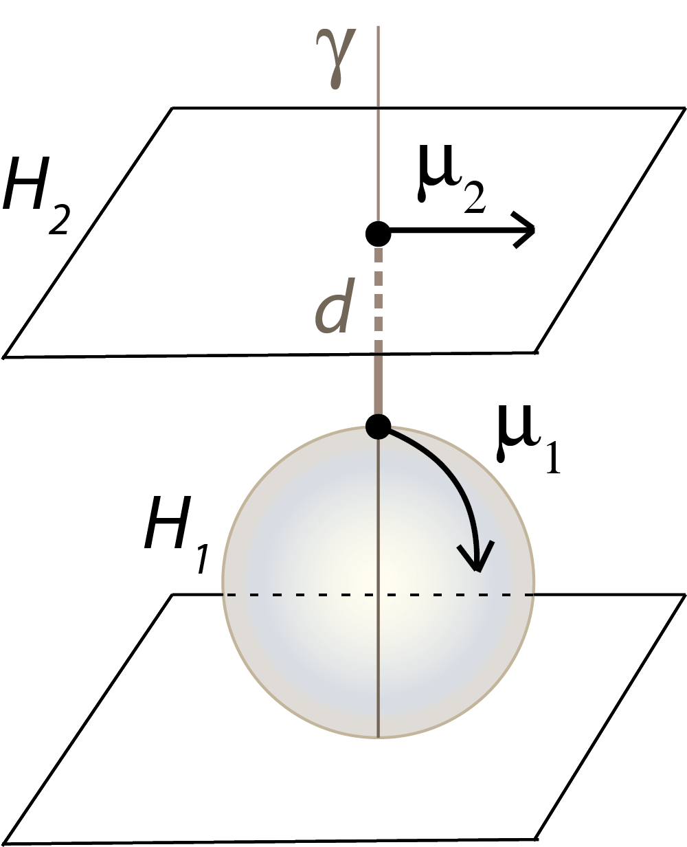
Observe that if we position one of $\displaystyle H_{1}$ and $\displaystyle H_{2}$ as $\displaystyle H_{\infty}$ and the other with center at $\displaystyle 0$ then the matrix

exchanges $\displaystyle H_{1}$ and $\displaystyle H_{2}$ taking meridian direction of $\displaystyle H_{1}$ to that of $\displaystyle H_{2}$.

We will also use another complex parameter defined as follows. Suppose we have three horospheres $\displaystyle H_{1}\neq H_{2}\neq H_{3}$, and $\displaystyle P_{i}$ is the center of a horosphere $\displaystyle H_{i}$ for $\displaystyle i=1,2,3$. Suppose $\displaystyle H_{2}$ intersects the geodesics $\displaystyle P_{1}P_{2}$ and $\displaystyle P_{2}P_{3}$ in points $\displaystyle N$ and $\displaystyle M$ respectively (see Fig. 2). Using the affine complex structure on $\displaystyle H_{2}$ there is a complex number determining a translation mapping $\displaystyle N$ to $\displaystyle M$. We call this complex number the translation parameter²² 2 In [14] certain translation parameters, sometimes with sign changed, are called “edge labels”. $\displaystyle u(H_{1},H_{2},H_{3})$. Note that if we position $\displaystyle H_{2}$ as $\displaystyle H_{\infty}$ then $\displaystyle u(H_{1},H_{2},H_{3})$ will be the complex number that corresponds to the translation between the centers $\displaystyle P_{1},P_{3}$ of $\displaystyle H_{1},H_{3}$. Then the matrix

gives a translation of $\displaystyle H_{2}$ taking $\displaystyle N$ to $\displaystyle M$.

We first give versions of Theorems 4.1 and 4.2 of [14] adapted to the orientation conventions of this paper, along with quick proofs of both. Let $\displaystyle H_{1},\dots,H_{n}$ be horospheres with $\displaystyle H_{i}\neq H_{i+1}$ for $\displaystyle i=1,\dots,n-1$ and $\displaystyle H_{n}\neq H_{1}$. We use the notation of equations (1) and (2),

As in [14] we use the shape parameter given by the cross ratio

which gives the parameter associated to the edge $\displaystyle P_{i}P_{i+1}$. In the literature this $\displaystyle\zeta$ is often associated with the vertex ordering $\displaystyle P_{i},P_{i+1},P_{i+2},P_{i-1}$.

If the image $\displaystyle\gamma_{ij}$ in $\displaystyle M$ of an intercusp geodesic arc $\displaystyle\gamma(H_{i},H_{j})$ is embedded we call $\displaystyle\gamma_{ij}$ an intercusp arc of $\displaystyle M$ and if the line segment in an $\displaystyle H_{j}$ joining the endpoints of a $\displaystyle\gamma(H_{i},H_{j})$ and a $\displaystyle\gamma(H_{j},H_{k})$ has embedded image $\displaystyle\gamma_{ijk}$ in $\displaystyle M$ we call $\displaystyle\gamma_{ijk}$ a cusp arc of $\displaystyle M$.

References

- [1] C. C. Adams, Waist size for cusps in hyperbolic 3-manifolds, Topology 41 (2002), no. 2, 257–270.
- [2] A. Borel, Commensurability classes and volumes of hyperbolic 3-manifolds, Ann. Scuola Norm. Sup. Pisa 8 (1981), 1–33.
- [3] D. Coulson; O. Goodman, C. Hodgson, W. D. Neumann, Computing arithmetic invariants of 3–manifolds, Experiment. Math. 9 (2000), no. 1, 127–152.
- [4] D. B. A. Epstein, R. C. Penner, Euclidean decompositions of noncompact hyperbolic manifolds, J. Diff. Geom. 27 (1988), 67–80.
- [5] H. M. Hilden, M. T. Lozano, J. M. Montesinos-Amilibia, A characterization of arithmetic subgroups of SL(2,R) and SL(2,C), Math. Nachr. 159 (1992), 245–270.
- [6] M. L. Macasieb, K. L. Petersen, R. M. van Luijk, On character varieties of two-bridge knot groups, Proc. Lond. Math. Soc. (3) 103 (2011), no. 3, 473–507.
- [7] C. Maclachlan, A. W. Reid, The arithmetic of hyperbolic 3-manifolds, Grad. Texts in Math., 219, Berlin, New York: Springer-Verlag (2003), 463 pp.
- [8] W. W. Menasco, Polyhedra representation of link complements, Low-dimensional topology (San Francisco, Calif., 1981), 305–325, Contemp. Math., 20, Amer. Math. Soc., Providence, RI, 1983.
- [9] D. Mostow, Quasi-conformal mappings in n-space and the rigidity of the hyperbolic space forms, Publ. Math. IHES 34 (1968), 53–104.
- [10] W. D. Neumann, A. W. Reid, Arithmetic of hyperbolic manifolds, in Topology ’90, Ohio State Univ. Math. Res. Inst. Publ. 1, de Gruyter, Berlin, (1992), 273–310.
- [11] G. Prasad, Strong rigidity of Q-rank 1 lattices, Invent. Math. 21 (1973), 255–286.
- [12] A. W. Reid, A note on trace-fields of Kleinian groups, Bull. London Math. Soc. 22 (1990), 349–352.
- [13] R. Riley, Parabolic representations of knot groups, I. Proc. London Math. Soc. (3) 24 (1972), 217–242.
- [14] M. Thistethwaite, A. Tsvietkova, An alternative approach to hyperbolic structures on link complements, to appear in Algebr. Geom. Topol., ArXiv: math.GT/1108.0510v1.
- [15] W. P. Thurston, The geometry and Topology of Three-Manifolds, Electronic Version 1.1 (March 2002), http://www.msri.org/publications/books/gt3m/
- [16] A. Tsvietkova, Hyperbolic links complements, Ph. D. Thesis, University of Tennessee, 2012.
- [17] A. Tsvietkova, Exact volume of hyperbolic 2-bridged links, to appear in Comm. Anal. Geom., ArXiv: math.GT/1211.5089
- [18] C. K. Zickert, The volume and Chern-Simons invariant of a representation, Duke Math. J. 150 (2009), no. 3, 489–532.