Collective oscillation period of inter-coupled biological negative cyclic feedback oscillators

We first consider the dynamics of a single negative cyclic feedback oscillator [20]:

Here $[\mathsf{P}_{m}]\in\mathbb{R}^{1}$ is the concentration of the product $\mathsf{P}_{m}$ (e.g., mRNA, protein, metabolite) in the $m$th reaction ($1\leq m\leq M$); $\rho_{m}$ ($0\leq m\leq M-1$) are the rates of synthesis; $k_{m}$ ($1\leq m\leq M$) are degradation rates; $1/K_{0}$ is the binding constant of the end product to the transcription factor; and $p$ is the Hill coefficient, which describes the cooperativity of end product repression.

The negative cyclic feedback oscillator in (1) can be transformed into a dimension-less form

by $\varsigma=\sqrt[M]{(\prod_{i=0}^{M-1}\rho_{i})/K_{0}},\>\>\nu_{M}=\frac{1}{K_{0}},\>\>\nu_{j-1}=\frac{\rho_{j-1}\nu_{i}}{\varsigma},\>\>x_{m}=\nu_{m}[\mathsf{P}_{m}],\>\>t=\varsigma T,$ and $b_{i}=\frac{\rho_{i}}{\varsigma}$ [20].

Transformation from (2) to (1) reduces parameters and thus facilitates an analytical treatment.

Next we consider a network of $N$ oscillators with each oscillator described by (2) (cf. Fig. 1). Following [22], we assume that one synchronizing factor (the $k$th reaction product $x_{k}$ ($2\leq k\leq M$)) connects the oscillators by diffusion. Then the network dynamics is given by

where $i=1,2,\ldots,N$ denotes the index of oscillator $i$, and $a_{i,j}\geq 0$ denotes the coupling strength between oscillators $i$ and $j$. If $a_{i,j}=0$, then there is no interaction between oscillators $i$ and $j$.

For convenience in analysis, we can recast (3) in the following matrix form:

Since $A$ is symmetric and has zero row-sums, it can be diagonalized by some matrix $P$:

where $0=\upsilon_{1}<\upsilon_{2}\leq\ldots\leq\upsilon_{N}$. The eigenvalue $0$ is associated with eigenvector $[1\>\>1\>\,\ldots\>\>1]^{T}$ [24]. $\upsilon_{2}$ measures the connectivity of interaction. It is positive when interaction is connected, and is greater when the interaction is stronger [24].

We are interested in the condition for oscillatory dynamics of the oscillator network in (4), so it is necessary to analyze its equilibrium. Next we show that (4) has one unique equilibrium.

At the equilibrium point, we have $dX_{m}^{\ast}/dt=0,\>m=\{1,2,\ldots,M\}$, which yields

Since the interaction is bi-directional, i.e., $a_{i,j}=a_{j,i}$, it follows

Next, we prove that (9) holds by proving that both $\max\limits_{i}\{g(x_{M,i}^{\ast})\}$ and $\min\limits_{i}\{g(x_{M,i}^{\ast})\}$ are zero:

Suppose to the contrary that (9) does not hold, then $\max\limits_{i}\{g(x_{M,i}^{\ast})\}>0$ since $\sum_{i=1}^{N}g(x_{M,i}^{\ast})=0$ holds according to (8). Represent the index of the largest $g(x_{M,i}^{\ast})$ among all $1\leq i\leq N$ as $q$. Then $x_{M,q}^{\ast}$ should be the smallest among $x_{M,1}^{\ast},\,x_{M,2}^{\ast},\ldots,x_{M,N}^{\ast}$ because $f(\bullet)$ and hence $g(\bullet)$ is a decreasing function (cf. definition in (7)). Therefore, the rightmost hand side of (7) should be non-positive, and hence $g(x_{M,q}^{\ast})<0$. This contradicts the fact that $g(x_{M,q}^{\ast})$ is the largest among $g(x_{M,i}^{\ast})$ and is positive (due to the constraint in (8)). Hence $\max\limits_{i}\{g(x_{M,i}^{\ast})\}=0$ holds. Similarly, we can prove $\min\limits_{i}\{g(x_{M,i}^{\ast})\}=0$. Therefore, we have (9), which further leads to

Since $f(x)$ is monotonic decreasing for $x\geq 0$, the solution to (10) is unique and it satisfies

Therefore the solution to (7) is unique, thus the equilibrium point is unique.

An oscillatory solution of (4) needs unstable dynamics near the equilibrium. To check the dynamics of (4) near the equilibrium, we linearize the nonlinear item $\vec{f}(X_{M})$ in (4) around $X_{M}^{\ast}$

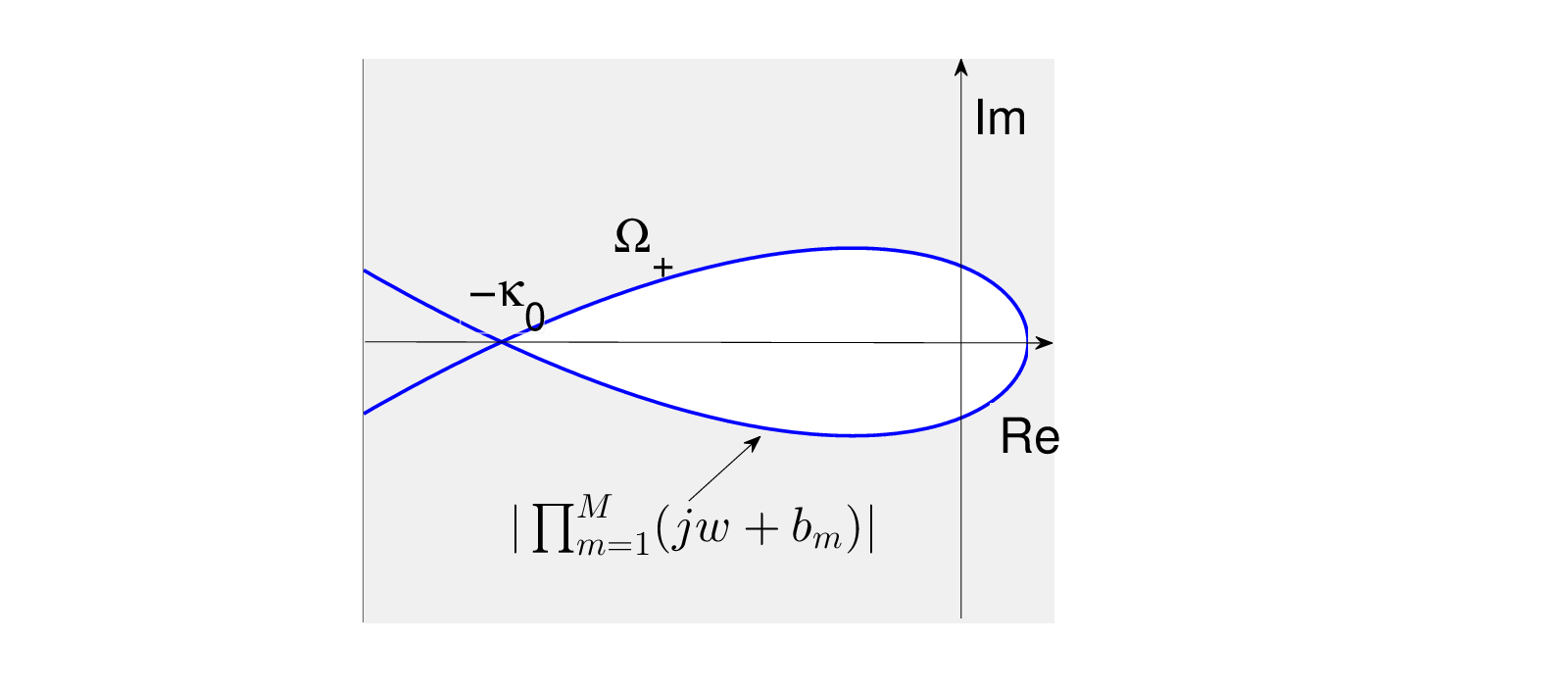
Then the overall dynamics of (4) can be represented in the frequency domain, as in Fig. 3, where

and the matrix $L\in\mathbb{R}^{N\times N}$ denotes the influence of the nonlinear term after linearization.

For a general matrix $L$, it is difficult to give an analytical treatment of the dynamics in Fig. 3. Fortunately, under the matrix formulation in (4), we can diagonalize the system and reduce it to multiple scalar subsystems. This is the key to derive the analytical results in this paper.

Using (4) and (12), we can get $L=\sigma I\in\mathbb{R}^{N\times N}$, and hence the overall dynamics in Fig. 3:

Substituting (6) into (13), we have

where $\lambda_{j}(s)=\frac{1}{(\prod_{m=1,m\neq k}^{M}(s+b_{m}))(s+b_{k}+\upsilon_{j})}$ for $j=1,2,\ldots,N.$ Substituting (15) into (14) yields

So far, we have decomposed the network dynamics into multiple scalar subsystems, which, as will be shown later, greatly facilitates an analytical treatment of the network dynamics.

To study the collective period, we need to guarantee that the $X_{m}$ in (4) oscillate, and furthermore, oscillate in synchrony. We consider the Y-oscillation, which is defined below [16]:

To prove that (4) is Y-oscillatory, we introduce Lemma 1:

The result follows from these considerations: To get Y oscillations, we need to guarantee that 1) the linearized systems near the equilibrium points do not converge to constant values; 2) the solutions are bounded; and, 3) there exists a homeomorphism between solutions of the nonlinear system and its linearization. All of these can be obtained following Theorem 1 in [25] and the discussion below its proof which shows that the hyperbolicity condition can be relaxed.

It can be verified that for $M\geq 2$, $R$ in (18) increases with $M$, the length of the cyclic feedback. Given that a larger $R$ makes (18) easier to satisfy, a longer cyclic feedback loop (i.e., a larger $M$, meaning involving more serial reactions) makes oscillation easier. Moreover, recalling the positive correlation between the averaged value of distributed delay and the length of feedback loop (cf. Remark 2), we can infer that a larger delay also makes oscillation easier.

From (21), we can see that with an increase in $z_{0}$, a larger $\upsilon_{2}$ (i.e., a stronger intercellular interaction) is required to achieve synchronization. Given that for $p>1$, $z_{0}$ can be verified an increasing function of the Hill coefficient $p$, we know that a system having a higher Hill coefficient (i.e., a higher cooperativity of end product repression) requires stronger coupling to maintain synchronization. Furthermore, we can also verify that a longer feedback chain makes the right hand side of the inequality in (21) lower, and thus makes (21) harder to satisfy. Given the positive correlation between the feedback loop length and the averaged distributed delay (cf. Remark 2), we can infer that a larger delay makes synchronization more difficult to maintain.

We reformulate the problem of oscillation analysis using a multivariable harmonic balance technique. This is motivated by the observation that $H(s)$ is a low pass filter thus higher order harmonics of oscillations in the closed-loop system can be safely neglected. Hence $x_{M,i}$ can be approximated by its zero-order and first-order harmonic components [16, 27]:

where $\alpha_{i}$ and $\beta_{i}$ denote the amplitudes of the zero-order and the first-order harmonic components, respectively, and $w$ and $\phi_{i}$ denote the oscillation frequency and phase, respectively.

Since $f(\bullet)$ is a static nonlinear function, it can be approximated by describing functions [27]:

The describing function $\xi_{i}$ is the gain of $f(\bullet)$ when the input is a constant $\alpha_{i}$ and the output is approximated by the zero-order harmonic component. The describing function $\eta_{i}$ is the gain of $f(\bullet)$ when the input is a sinusoid of amplitude $\beta_{i}$ and the output is approximated by the first-order harmonic component [27].

Consequently, $\alpha_{i}$ and $\beta_{i}$ are expected to satisfy [16]:

where $\Xi=\textrm{diag}\{\xi_{1},\,\ldots,\xi_{N}\}\in\mathbb{R}^{N\times N}$, $\Pi=\textrm{diag}\{\eta_{1},\,\ldots,\eta_{N}\}\in\mathbb{R}^{N\times N}$, and

Note that (29) are referred to as harmonic balance equations.

Let $\Xi^{\ast}$ and $\Pi^{\ast}$ be matrices satisfying (29). Define two linear systems $G_{0}(s)$ and $G_{1}(s)$ as

$G_{0}(s)$ and $G_{1}(s)$ are obtained by replacing the nonlinearity $f(\bullet)$ with the constant gain computed from the describing functions. To ensure that the predicted oscillation frequency is biologically significant, oscillations at the estimated frequency must be stable, which, according to [28], can be ensured if both $G_{0}(s)$ and $G_{1}(s)$ are marginally stable (the only unstable poles are $s=0$ and $s=\pm jw$, respectively). Therefore, estimating the collective period can be reduced to:

Eqn (29) is very difficult to solve since in general $\Xi$ and $\Pi$ depend on $\vec{\alpha}$ and $\vec{\beta}$. Keeping in mind that we are interested in the collective period, we concentrate on solutions that describe synchronized oscillations. According to Definition 2, synchrony means that $x_{M,i}$ are identical, i.e., 1) the phases $\phi_{i}$ are identical; 2) the amplitudes $\alpha_{i}$ and $\beta_{i}$ are respectively identical. Given that $\xi_{i}$ and $\eta_{i}$ are determined by $\alpha_{i}$ and $\beta_{i}$, we further have the equality of all $\xi_{i}$ and all $\eta_{i}$:

where $\alpha$, $\beta$, $\xi$, and $\eta$ are constants. Hence (29) reduces to

which further means that $\frac{1}{\xi}$ and $\frac{1}{\eta}$ are the respective eigenvalues of $H(0)$ and $H(jw)$ corresponding to the eigenvector with identical elements.

From (15), we know the eigenvalues of $H(0)$ are $\lambda_{j}=\frac{1}{(b_{k}+\upsilon_{j})(\prod_{m=1,m\neq k}^{M}b_{m})}$ for $j=1,2,\ldots,N$. Since only $\lambda_{1}$ corresponds to eigenvectors with identical elements, we have (note $\upsilon_{1}=0$)

Similarly, we can get that the eigenvalues of $H(jw)$ are $\lambda_{j}(jw)=\frac{1}{(jw+b_{k}+\upsilon_{j})\prod_{m=1,m\neq k}^{M}(jw+b_{m})}$ for $j=1,2,\ldots,N$. Since only $\lambda_{1}$ corresponds to eigenvectors with identical elements, we have

According to (28), $\eta$ is real, thus the right hand side of (34) must be real. Given that $\mu$ is the minimal frequency that makes $\prod_{m=1}^{M}(jw+b_{m})$ have zero imaginary part (angular $\pi$), the collective frequency is determined by $\mu$ in (19) and

To solve Problem 1, it remains to prove that $G_{0}(s)$ and $G_{1}(s)$ in (30) are marginally stable [28], or in other words: (1) $G_{0}(s)$ has one pole of $s=0$ and the rest in the open left half plane and, (2) $G_{1}(s)$ has imaginary poles $s=\pm jw$ and the rest in the open left half plane.

Substituting $\Xi$ and $\Pi$ in (31) into (30) yields

with $\xi$ and $\eta$ given in (33) and (35), respectively.

First consider $G_{0}(s)$. From (16)-(17), we know that the eigenvalues of $G_{0}(s)$ are given by

Substituting $\xi$ in (33) into (37), we know that the poles of $G_{0}(s)$ in (36) are the roots of

For $j=1$, since $\upsilon_{1}=0$, (38) has one root $s=0$. It can also be derived that all the rest of the roots have negative real parts since for all $s$ with a positive real part, the modulus of $\prod_{m=1}^{M}b_{m}$ is less than $\prod_{m=1}^{M}(s+b_{m})$, which makes equality in (38) impossible. Similarly, we can get that for $j\neq 1$, all roots of (38) have negative real parts. Hence $G_{0}(s)$ is marginally stable.

Following the same line of reasoning, we can prove that the eigenvalues of $G_{1}(s)$ are

with $\eta$ given in (35). And hence its poles are determined by the roots of

where $\mu$ is given in (19).

For $j=1$, we can verify that $s=\pm jw$ are roots of (39). We can also verify that all the other roots of (39) are stable, since for all $s$ with a positive real part, the intersection of $\prod_{m=1}^{M}(s+b_{m})$ and the negative real axis is less than $-\kappa_{0}\hskip-2.84544pt=\hskip-2.84544pt-\hskip-2.84544pt\prod\limits_{m=1}^{M}\hskip-4.26773pt\sqrt{\mu^{2}+b_{m}^{2}}$, which makes the equality in (39) impossible. Similarly, for $j\neq 1$, we can derive that all roots of (39) are in the open left half plane. So $G_{1}(s)$ is marginally stable. Hence oscillations at the derived frequency $\mu$ are stable.

From the above derivation, we can see that the collective oscillation period is expected to be

The collective period in (40) is given in terms of the dimensionless parameters in (2). The actual collective frequency in dimensional parameters are given by $\Omega=\varsigma\mu$ where $\mu$ is the minimal positive solution to $\sum\limits_{m=1}^{M}\arctan\frac{\mu}{b_{m}}=\sum\limits_{m=1}^{M}\arctan\frac{\mu}{k_{m}/\varsigma}=\pi.$ So the actual collective frequency is the minimal positive solution to $\sum\limits_{m=1}^{M}\arctan\frac{\Omega}{k_{m}}=\pi$. This means that the collective frequency $\Omega$ increases with an increase in the degradation rate of each component ($k_{m}$), but it is independent of the rates of transcription, translation, and synthesis. These give insights into the basic determination mechanism of the collective period in coupled biological oscillators, and may further provide guidance in synthetic biology design.

From the above derivation, we can see that under interaction (3), the collective period is only determined by $k_{m}$ ($m=1,2,\ldots,M$), and it is independent of intercellular coupling. The results are obtained based on analytical treatment of a network of coupled gene regulatory oscillators and they corroborate the results in [15], which are obtained using the phenomenological single-variable phase model and state that the strength of intercellular coupling does not affect the collective period of circadian rhythm oscillator networks. In fact, this is reasonable since the coupling is similar to the linear consensus protocol [29], which only affects the process to synchronization. Moreover, when the degradation rate is fixed, it can be inferred that $\Omega$ decreases with an increase in the length of the feedback loop $M$. Therefore, a longer feedback loop corresponds to a longer collective period. Furthermore, recall that the effect of distributed delay amounts to increasing the length of the feedback loop and the increased length is proportional to the averaged delay, hence, a larger delay in individual loops means a longer collective period.

References

- [1] Y. Q. Wang, Y. Hori, S. Hara, and F. J. Doyle III. The collective oscillation period of inter-coupled goodwin oscillators. In Proc. 51th IEEE Conf. Decision Control, pages 1627–1632, Maui, USA, 2012.
- [2] O. V. Popovych and P. A. Tass. Macroscopic entrainment of periodically forced oscillatory ensembles. Prog. Biophys. Mol. Biol., 105:98–108, 2011.
- [3] H Wünsche, S Bauer, J Kreissl, O Ushakov, N Korneyev, F Henneberger, E Wille, H Erzgräber, M Peil, W Elsäßer, and I Fischer. Synchronization of delay-coupled oscillators: a study of semiconductor lasers. Phys. Rev. Lett., 94:163901, 2005.
- [4] L. Herrgen, S. Ares, L. G. Morelli, C. Schröter, F. Jülicher, and A. C. Oates. Intercellular coupling regulates the period of the segmentation clock. Curr. Biol., 20:1244–1253, 2010.
- [5] B. Novák and J. J. Tyson. Design principles of biochemical oscillators. Nat. Rev. Mol. Cell Biol., 9:981–991, 2008.
- [6] C. Fall, E. Marland, J. Wagner, and J. J. Tyson, editors. Computational Cell Biology. Springer, New York, 2005.
- [7] N. Stephanopoulos, A. Aristidou, and J. Nielsen, editors. Metabolic engineering principles and methodologies. Academic Press, San Diego, 1998.
- [8] J. Griffith. Mathematics of cellular control processes: negative feedback to one gene. J. Theoret. Biol., 20:202–208, 1968.
- [9] A. Hunding. Limit-cycles in enzyme-systems with nonlinear negative feedback. Biophys Struct Mech., 1:47–54, 1974.
- [10] J. Tyson. On the existence of oscillatory solutions in negative feedback cellular control processes. J. Math. Biol., 1:311–315, 1975.
- [11] Y. Hori, T. Kim, and S. Hara. Existence criteria of periodic oscillations in cyclic gene regulatory networks. Automatica, 47:1203–1209, 2011.
- [12] A. Hamadeh, G. Stan, R. Sepulchre, and J. Goncalves. Global state synchronization in networks of cyclic feedback systems. IEEE Trans. Autom Control, 57:478–483, 2012.
- [13] P. Papp. Analysis of biochemical phase shift oscillators by a harmonic balancing technique. Math Biol, 25:203–224, 1976.
- [14] Y. Hori, M. Takada, and S. Hara. Biochemical oscillations in delayed negative cyclic feedback: Existence and profiles. Automatica, 49:2581–2590, 2013.
- [15] C. Liu, D. Weaver, S. H. Strogatz, and S. M. Reppert. Cellular construction of a circadian clock: period determination in the Suprachiasmatic Neuclei. Cell, 91:855–860, 1997.
- [16] T. Iwasaki. Multivariable harmonic balance for central pattern generators. Automatica, 44:3061–3069, 2008.
- [17] A. Turing. The chemical basis of morphogenesis. Phil. Trans. R. Soc. B, 237:37–72, 1952.
- [18] Y. Q. Wang, Y. Hori, S. Hara, and F. J. Doyle III. Intercellular delay regulates the collective period of repressively coupled gene regulatory oscillator networks. IEEE Trans. Autom. Control, 59:211–216, 2014.
- [19] N. MacDonald. Time lags in biological models. Springer, Berlin, 1978.
- [20] J. Tyson and H. Othmer. The dynamics of feedback control circuits in biochemical pathways. Prog. Theo. Biol., 5:1–62, 1978.
- [21] J. J. Tyson. Periodic enzyme synthesis reconsideration of the theory of oscillatory repression. J. Theor. Biol., 80:27–38, 1979.
- [22] N. Bagheri, S. Taylor, K. Meeker, L. Petzold, and F. J. Doyle III. Synchrony and entrainment properties of robust circadian oscillators. J. R. Soc. Interface, 5:S17–S28, 2008.
- [23] T. To, M. A. Henson, E. Herzog, and F. J. Doyle. A molecular model for intercellular synchronization in the mammalian circadian clock. Biophys. J., 92:3792–3803, 2007.
- [24] R. Horn and C. Johnson. Matrix analysis. Cambridge University Press, London, 1985.
- [25] A. Pogromsky, T. Glad, and H. Nijmeijer. On diffusion driven oscillations in coupled dynamical systems. Int. J. Bifurcation Chaos, 9:629–644, 1999.
- [26] H. El Samad, D. Del Vecchio, and M. Khammash. Repressilators and promotilators: loop dynamics in synthetic gene networks. In Proc. 2005 American Contr. Conf., pages 4405–4410, Portland, USA, 2005.
- [27] H. K. Khalil. Nonlinear systems. Prentice Hall, New Jersey, 2002.
- [28] T. Glad and L. Ljung. Control theory - multivariable and nonlinear methods. Taylor & Francis, 2000.
- [29] R. Olfati-Saber, J. A. Fax, and R. M. Murray. Consensus and cooperation in networked multi-agent systems. Proc. IEEE, 95:215–233, 2007.