An efficient numerical method for acoustic wave scattering in random media

Xiaobing Feng ^†^†thanks: Department of Mathematics, The University of Tennessee, Knoxville, TN 37996, U.S.A. (xfeng@math.utk.edu) The work of this author was partially supported by the NSF grants DMS-1016173 and DMS-1318486. Junshan Lin ^†^†thanks: Department of Mathematics and Statistics, Auburn University, Auburn, AL 36849, U.S.A. (jzl0097@auburn.edu) Cody Lorton ^†^†thanks: Department of Mathematics, The University of Tennessee, Knoxville, TN 37996, U.S.A. (lorton@math.utk.edu) The work of this author was partially supported by the NSF grants DMS-1016173 and DMS-1318486.

Abstract

This paper is concerned with developing efficient numerical methods for acoustic wave scattering in random media which can be expressed as random perturbations of homogeneous media. We first analyze the random Helmholtz problem by deriving some wave-number-explicit solution estimates. We then establish a multi-modes representation of the solution as a power series of the perturbation parameter and analyze its finite modes approximations. Based on this multi-modes representation, we develop a Monte Carlo interior penalty discontinuous Galerkin (MCIP-DG) method for approximating the mode functions, which are governed by recursively defined nearly deterministic Helmholtz equations. Optimal order error estimates are derived for the method and an efficient algorithm, which is based on the LU direct solver, is also designed for efficiently implementing the proposed multi-modes MCIP-DG method. It is proved that the computational complexity of the whole algorithm is comparable to that of solving one deterministic Helmholtz problem using the LU director solver. Numerical experiments are provided to validate the theoretical results and to gauge the performance of the proposed numerical method and algorithm.

keywords

Helmholtz equation, random media, Rellich identity, discontinuous Galerkin method, error estimate, LU decomposition, Monte Carlo method.

AMS

65N12, 65N15, 65N30,

1 Introduction

Partial differential equations with random coefficients arise naturally in the modeling of many physical phenomena. This is due to the fact that some level of uncertainty is usually involved if the knowledge of the physical behavior is not complete or when noise is present in the experimental measurements. In recent years, substantial progress has been made in the numerical approximation of such PDEs due to the significant development in computational resources. We refer to [1, 2, 3, 15, 16] and references therein for more details.

In this paper, we consider the propagation of the acoustic wave in a medium where the wave velocity is characterized by a random process. More precisely, we study the approximation of the solution to the following Helmholtz problem:

(1)		$\displaystyle-\Delta u(\omega,\cdot)-k^{2}\alpha(\omega,\cdot)^{2}u(\omega,\cdot)$	$\displaystyle=f(\omega,\cdot)$		$\displaystyle\qquad\mbox{in }D,$
(2)		$\displaystyle\partial_{\nu}u(\omega,\cdot)+{\rm\mathbf{i}}k\alpha(\omega,\cdot)u(\omega,\cdot)$	$\displaystyle=0$		$\displaystyle\qquad\mbox{on }\partial D,$

where $k$ is the wavenumber, and $D\subset\mathbb{R}^{d}\,(d=1,2,3)$ is a convex bounded polygonal domain with boundary $\partial D$ . Let $(\Omega,\mathcal{F},P)$ be a probability space with sample space $\Omega$ , $\sigma-$ algebra $\mathcal{F}$ and probability measure $P$ . For each fixed $x\in D$ , the refractive index $\alpha(\cdot,x)$ is a real-valued random variable defined over $\Omega$ . We assume that the medium is a small random perturbation of a uniform background medium in the sense that

(3)

\displaystyle\alpha(\omega,\cdot):=1+\varepsilon\eta(\omega,\cdot).

Here $\varepsilon$ represents the magnitude of the random fluctuation, and $\eta\in L^{2}(\Omega,L^{\infty}(D))$ is some random process satisfying

P\left\{\omega\in\Omega;\,\left\|\eta(\omega,\cdot)\right\|_{L^{\infty}(D)}\leq 1\right\}=1.

For notation brevity we only consider the case that $\eta$ is real-valued. However, we note that the results of this paper are also valid for complex-valued $\eta$ . On the boundary $\partial D$ , a radiation boundary condition is imposed to absorb incoming waves [6]. Here $\nu$ denotes the unit outward normal to $\partial D$ , and $\partial_{\nu}u$ stands for the normal derivative of $u$ . The boundary value problem (1)–(2) arises in the modeling of the wave propagation in complex environments, such as composite materials, oil reservoir and geological basins [9, 12]. In such instances, it is of practical interest to characterize the uncertainty of the wave energy transport when the medium contains some randomness. In particular, we are interested in the computation of some statistics of the wave field, e.g, the mean value of the solution $u$ .

To solve stochastic (or random) partial differential equations (SPDEs) numerically, the simplest and most natural approach is to use the Monte Carlo method, where a set of independent identically distributed (i.i.d.) solutions are obtained by sampling the PDE coefficients, and the mean of the solution is calculated via a statistical average over all the sampling in the probability space [3]. An alternative is the stochastic Galerkin method, where the SPDE is reduced to a high dimensional deterministic equation by expanding the random field in the equation using the Karhunen-Loève or Wiener Chaos expansions. We refer the reader to [1, 2, 5, 15, 16] for detailed discussions. However, it is known that a brute-force Monte Carlo or stochastic Galerkin method applied directly to the Helmholtz equation with random coefficients is computationally prohibitive even for a moderate wavenumber $k$ , since a large number of degrees of freedom is involved in the spatial discretization. It is apparent that in such cases, the Monte Carlo method requires solving a PDE with many sampled coefficients, while the high dimensional deterministic equation associated with the stochastic Galerkin method will be too expensive to be solved.

In this paper, we propose an efficient numerical method for solving the Helmholtz problem (1)–(2) when the medium is weakly random defined by (3). A multi-modes representation of the solution is derived, where each mode is governed by a Helmholtz equation with deterministic coefficients and a random source. We develop a Monte Carlo interior penalty discontinuous Galerkin (MCIP-DG) method for approximating the mode functions. In particular, we take the advantage that the coefficients of the Helmholtz equation for all the modes are identical, hence the associated discretized equations share the same constant coefficient matrix. Using this crucial fact, it is observed that an LU direct solver for the discretized equations leads to a tremendous saving in the computational costs, since the LU decomposition matrices can be used repeatedly, and the solutions for all modes and all samples can be obtained in an efficient way by performing simple forward and backward substitutions. Indeed, it turns out that the computational complexity of the proposed algorithm is comparable to that of solving one deterministic Helmholtz problem using the LU direct solver.

The rest of the paper is organized as follow. A wave-number-explicit estimate for the solution of the random Helmholtz equation is established in Section 2. In Section 3, we introduce the multi-modes expansion of the solution as a power series of $\varepsilon$ and analyze the error estimation for its finite-modes approximation. The Monte Carlo interior penalty discontinuous Galerkin method is presented in Section 4, where the error estimates for the approximation of each mode function is also obtained. In Section 5, a numerical procedure for solving (1)–(2) is described and its computational complexity is analyzed in detail. In addition, we derive an optimal order error estimates for the proposed procedure. Several numerical experiments are provided in Section 6 to demonstrate the efficiency of the method and to validate the theoretical results.

2 PDE analysis

2.1 Preliminaries

Standard function and space notations are adopted in this paper. For example, $H^{s}(D)$ denotes the complex-valued Sobolev space and $L^{2}(D)=H^{0}(D)$ . $(\cdot,\cdot)_{S}$ stands for the standard inner product on the complex-valued $L^{2}(S)$ space for any subset $S$ of $D$ . $\,C$ and $c$ denote generic constants which are independent of $k$ and the mesh parameter $h$ . We also define spaces

(4)		$\displaystyle H^{1}_{+}(D)$	$\displaystyle:=\bigl\{v\in H^{1}(D);\,\|\nabla v\|\bigr\|_{\Gamma}\in L^{2}(\partial D)\bigr\},$
(5)		$\displaystyle V$	$\displaystyle:=\big\{v\in H^{1}(D);\,\Delta v\in L^{2}(D)\bigr\}.$

Without loss of generality, we assume that the domain $D\subset B_{R}(0)$ . Throughout this paper we also assume that $D$ is a star-shaped domain with respect to the origin in the sense that there exists a positive constant $c_{0}$ such that

x\cdot\nu\geq c_{0}\quad\mbox{on }\partial D,

Let $(\Omega,\mathcal{F},P)$ be a probability space on which all the random variables of this paper are defined. $\mathbb{E}(\cdot)$ denotes the expectation operator. The abbreviation a.s. stands for almost surely.

As it will be needed in the late sections of the paper, in this section we analyze the boundary value problem for the Helmholtz equation (1) with the following slightly more general nonhomogeneous boundary condition:

(6)

\partial_{\nu}u(\omega,\cdot)+{\rm\mathbf{i}}k\alpha(\omega,\cdot)u(\omega,\cdot)=g(\omega,\cdot).

Definition 1.

Let $f\in L^{2}(\Omega,L^{2}(D))$ and $g\in L^{2}(\Omega,L^{2}(\partial D))$ . A function $u\in L^{2}(\Omega,H^{1}(D))$ is called a weak solution to problem (1),(6) if it satisfies the following identity:

(7)

\int_{\Omega}a(u,v)\,dP=\int_{\Omega}\big((f,v)_{D}+\langle g,v\rangle_{\partial D}\big)\,dP\qquad\forall v\in L^{2}(\Omega,H^{1}(D)),

where

(8)

\displaystyle a(w,v)

\displaystyle:=\bigl(\nabla w,\nabla v\bigr)_{D}-k^{2}\bigl(\alpha^{2}w,v\bigr)_{D}+{\rm\mathbf{i}}k\left\langle\alpha w,v\right\rangle_{\partial D}.

Remark 2.1.

Using (10) below, it is easy to show that any solution $u$ of (1),(6) satisfies $u\in L^{2}(\Omega,H^{1}_{+}(D)\cap V)$ .

2.2 Wave-number-explicit solution estimates

In this subsection we shall derive stability estimates for the solution of problem (1),(6) which is defined in Definition 1. Our focus is to obtain explicit dependence of the stability constants on the wave number $k$ , such wave-number-explicit stability estimates will play a vital role in our convergence analysis in the later sections. We note that wave-number-explicit stability estimates also play a pivotal role in the development of numerical methods, such as finite element and discontinuous Galerkin methods, for deterministic reduced wave equations (cf. [7, 8]). As a byproduct of the stability estimates, the existence and uniqueness of solutions to problem (1),(6) can be conveniently established.

Lemma 2.

Let $u\in L^{2}(\Omega,H^{1}(D))$ be a solution of (1),(6), then for any $\delta_{1},\delta_{2}>0$ and $\varepsilon<1$ there hold

(9)	$\displaystyle\mathbb{E}(\left\\|\nabla u\right\\|_{L^{2}(D)}^{2})$	$\displaystyle\leq\Bigl(k^{2}(1+\varepsilon)^{2}+\delta_{1}\Bigr)\mathbb{E}(\left\\|u\right\\|_{L^{2}(D)}^{2})$
	$\displaystyle\qquad+\left(\frac{\delta_{1}}{2k^{2}(1-\varepsilon)^{2}}+\frac{1}{2\delta_{1}}\right)\left(\mathbb{E}(\left\\|f\right\\|_{L^{2}(D)}^{2})+\mathbb{E}(\left\\|g\right\\|_{L^{2}(\partial D)}^{2})\right),$
(10)	$\displaystyle\mathbb{E}(\left\\|u\right\\|_{L^{2}(\partial D)}^{2})$	$\displaystyle\leq\frac{\delta_{2}}{k(1-\varepsilon)}\mathbb{E}(\left\\|u\right\\|_{L^{2}(D)}^{2})+\frac{1}{\delta_{2}k(1-\varepsilon)}\mathbb{E}(\left\\|f\right\\|_{L^{2}(D)}^{2})$
	$\displaystyle\qquad+\frac{1}{k^{2}(1-\varepsilon)^{2}}\mathbb{E}(\left\\|g\right\\|_{L^{2}(\partial D)}^{2}).$

Proof.

Setting $v=u$ in (7) yields

\int_{\Omega}a(u,u)\,dP=\int_{\Omega}\big((f,u)_{D}+\langle g,v\rangle_{\partial D}\big)\,dP

Taking the real and imaginary parts and using the definition of $a(\cdot,\cdot)$ , we get

(11)		$\displaystyle\int_{\Omega}\Bigl(\\|\nabla u\\|_{L^{2}(D)}^{2}-k^{2}(1+\varepsilon\eta)^{2}\\|u\\|_{L^{2}(D)}^{2}\Bigr)\,dP$	$\displaystyle={\rm Re}\int_{\Omega}\big((f,u)_{D}+\langle g,v\rangle_{\partial D}\big)\,dP,$
(12)		$\displaystyle k\int_{\Omega}\langle 1+\varepsilon\eta,\|u\|^{2}\rangle_{\partial D}\,dP$	$\displaystyle={\rm Im}\int_{\Omega}\big((f,u)_{D}+\langle g,v\rangle_{\partial D}\big)\,dP.$

Applying the Cauchy-Schwarz inequality to (12) produces

	$\displaystyle k(1-\varepsilon)\mathbb{E}(\\|u\\|_{L^{2}(\partial D)}^{2})$	$\displaystyle\leq\frac{\delta_{2}}{2}\mathbb{E}(\\|u\\|_{L^{2}(D)}^{2})+\frac{1}{2\delta_{2}}\mathbb{E}(\\|f\\|_{L^{2}(D)}^{2})$
		$\displaystyle\qquad+\frac{k(1-\varepsilon)}{2}\mathbb{E}(\\|u\\|_{L^{2}(\partial D)}^{2})+\frac{1}{2k(1-\varepsilon)}\mathbb{E}(\\|g\\|_{L^{2}(\partial D)}^{2})$

Thus, (10) holds. Applying Cauchy-Schwarz to (11) yields

	$\displaystyle\mathbb{E}(\\|\nabla u\\|_{L^{2}(D)}^{2})$	$\displaystyle\leq\left(k^{2}(1+\varepsilon)^{2}+\frac{\delta_{1}}{2}\right)\mathbb{E}(\\|u\\|_{L^{2}(D)}^{2})+\frac{1}{2\delta_{1}}\mathbb{E}(\\|f\\|_{L^{2}(D)}^{2})$
		$\displaystyle\qquad+\frac{\delta_{1}}{2}\mathbb{E}(\\|u\\|_{L^{2}(\partial D)}^{2})+\frac{1}{2\delta_{1}}\mathbb{E}(\\|g\\|_{L^{2}(\partial D)}^{2}).$

To this one can apply (10) with $\delta_{2}=k(1-\varepsilon)$ and obtain (9). The proof is complete. ∎

Lemma 3.

Let $u\in L^{2}(\Omega,H^{2}(D))$ , then there hold

(13)	$\displaystyle{\rm Re}\int_{\Omega}\bigl(u,x\cdot\nabla u\bigr)_{D}\,dP$	$\displaystyle=-\frac{d}{2}\int_{\Omega}\\|u\\|_{L^{2}(D)}^{2}\,dP+\frac{1}{2}\int_{\Omega}\langle x\cdot\nu,\|u\|^{2}\rangle_{\partial D}\,dP,$
(14)	$\displaystyle{\rm Re}\int_{\Omega}\bigl(\nabla u,\nabla(x\cdot\nabla u)\bigr)_{D}\,dP$	$\displaystyle=\frac{2-d}{2}\int_{\Omega}\\|\nabla u\\|_{L^{2}(D)}^{2}\,dP$
	$\displaystyle\hskip 57.81621pt+\frac{1}{2}\int_{\Omega}\left\langle x\cdot\nu,\|\nabla u\|^{2}\right\rangle_{\partial D}\,dP.$

Proof.

(13) follows immediately from applying the divergence theorem to

\int_{\Omega}\bigl({\rm div}(x|u|^{2}),1\bigr)_{D}\,dP,

and the fact that ${\rm div}(x)=d$ . To show (14), we first recall the following differential identities [4]:

	$\displaystyle\nabla\cdot(x\|\nabla u\|^{2})$	$\displaystyle=d\|\nabla u\|^{2}+x\cdot\nabla(\|\nabla u\|^{2}),$
	$\displaystyle x\cdot\nabla(\|\nabla u\|^{2})$	$\displaystyle=2{\rm Re}\Bigl(\nabla\cdot(\nabla u(\overline{x\cdot\nabla u}))-\Delta u(\overline{x\cdot\nabla u})\Bigr)-2\|\nabla u\|^{2}$
		$\displaystyle=2{\rm Re}\bigl(\,\nabla u\cdot\overline{\nabla(x\cdot\nabla u)}\,\bigr)-2\|\nabla u\|^{2}.$

Then (14) follows from adding the above two identities, integrating the sum over $D\times\Omega$ and applying the divergence theorem on the left-hand side of the resulting equation. ∎

Remark 2.2.

(14) could be called a stochastic Rellich identity for the Laplacian.

We are now ready to state and prove our wave-number-explicit estimate for solutions of problem (1),(6) defined in Definition 1.

Theorem 4.

Let $u\in L^{2}(\Omega,H^{1}(D))$ be a solution of (1),(6) and $R$ be the smallest number such that $B_{R}(0)$ contains the domain $D$ . Then there hold the following estimates:

(15)		$\displaystyle\mathbb{E}\Bigl(\left\\|u\right\\|_{L^{2}(D)}^{2}+\left\\|u\right\\|_{L^{2}(\partial D)}^{2}+c_{0}\left\\|\nabla u\right\\|_{L^{2}(\partial D)}^{2}\Bigr)$	$\displaystyle\leq C_{0}\Bigl(\frac{1}{k}+\frac{1}{k^{2}}\Bigr)^{2}M(f,g),$
(16)		$\displaystyle\mathbb{E}(\left\\|u\right\\|_{H^{1}(D)}^{2})$	$\displaystyle\leq C_{0}\Bigl(1+\dfrac{1}{k^{2}}\Bigr)^{2}M(f,g),$

provided that $\varepsilon(2+\varepsilon)<\gamma_{0}:=\min\bigl\{1,\frac{13-2d}{2(4d-7)+25kR}\bigr\}$ . Where $C_{0}$ is some positive constant independent of $k$ and $u$ , and

(17)

M(f,g):=\mathbb{E}\Bigl(\left\|f\right\|_{L^{2}(D)}^{2}+\left\|g\right\|_{L^{2}(\partial D)}^{2}\Bigr).

Moreover, if $g\in L^{2}(\Omega,H^{\frac{1}{2}}(D))$ and $u\in L^{2}(\Omega,H^{2}(D))$ , there also holds

(18)

\displaystyle\mathbb{E}(\left\|u\right\|_{H^{2}(D)}^{2})\leq C\Bigl(k+\dfrac{1}{k^{2}}\Bigr)^{2}\mathbb{E}\Bigl(\left\|f\right\|_{L^{2}(D)}^{2}+\left\|g\right\|_{H^{\frac{1}{2}}(\partial D)}^{2}\Bigr).

Proof.

To avoid some technicalities, below we only give a proof for the case $u\in L^{2}(\Omega,H^{2}(D))$ . For the general case, $u$ needs be replaced by its mollification $u_{\rho}$ at the beginning of the proof and followed by taking the limit $\rho\to 0$ after the integration by parts is done.

Setting $v=x\cdot\nabla u$ in (7) yields

(19)

\int_{\Omega}\Bigl((\nabla u,\nabla v)_{D}-k^{2}(\alpha^{2}u,v)_{D}+{\rm\mathbf{i}}k\langle\alpha u,v\rangle_{\partial D}\Bigr)\,dP=\int_{\Omega}\left((f,v)_{D}+\langle g,v\rangle_{\partial D}\right)\,dP.

Using (13) and (14) after taking the real part of (19) and regrouping we get

		$\displaystyle\dfrac{dk^{2}}{2}\int_{\Omega}\\|u\\|_{L^{2}(D)}^{2}\,dP=\int_{\Omega}\Bigl(\frac{d-2}{2}\\|\nabla u\\|_{L^{2}(D)}^{2}+k^{2}\varepsilon\,{\rm Re}\bigl(\eta(2+\varepsilon\eta),v\bigr)_{D}\Bigr)\,dP$
		$\displaystyle\hskip 43.36243pt-\int_{\Omega}\Bigl(k{\rm Im}\langle(1+\varepsilon\eta)u,v\rangle_{\partial D}+\frac{1}{2}\left\langle x\cdot\nu,\|\nabla u\|^{2}\right\rangle_{\partial D}-\frac{k^{2}}{2}\left\langle x\cdot\nu,\|u\|^{2}\right\rangle_{\partial D}\Bigr)\,dP$
		$\displaystyle\hskip 43.36243pt+\int_{\Omega}\left({\rm Re}(f,v)_{D}+{\rm Re}\langle g,v\rangle_{\partial D}\right)\,dP$

It then follows from Schwarz inequality and the “star-shape” condition and the facts that $|x|\leq R$ for $x\in D$ and $\|\eta\|_{L^{\infty}(D)}\leq 1$ a.s. that

	$\displaystyle\frac{dk^{2}}{2}\mathbb{E}(\left\\|u\right\\|_{L^{2}(D)}^{2})$	$\displaystyle\leq\frac{d-2}{2}\mathbb{E}(\left\\|\nabla u\right\\|_{L^{2}(D)}^{2})+k^{2}\varepsilon R(2+\varepsilon)\Bigl(\frac{1}{2\delta_{1}}\mathbb{E}(\left\\|u\right\\|_{L^{2}(D)}^{2})$
		$\displaystyle\qquad+\frac{\delta_{1}}{2}\mathbb{E}(\left\\|\nabla u\right\\|_{L^{2}(D)}^{2})\Bigr)+\frac{R}{2\delta_{2}}\mathbb{E}(\left\\|f\right\\|_{L^{2}(D)}^{2})+\frac{R\delta_{2}}{2}\mathbb{E}(\left\\|\nabla u\right\\|_{L^{2}(D)}^{2})$
		$\displaystyle\qquad+\frac{R}{2\delta_{3}}\mathbb{E}(\left\\|g\right\\|_{L^{2}(\partial D)}^{2})+\frac{R\delta_{3}}{2}\mathbb{E}(\left\\|\nabla u\right\\|_{L^{2}(\partial D)}^{2})$
		$\displaystyle\qquad+\frac{kR}{\delta_{4}}\mathbb{E}(\left\\|u\right\\|_{L^{2}(\partial D)}^{2})+kR\delta_{4}\mathbb{E}(\left\\|\nabla u\right\\|_{L^{2}(\partial D)}^{2})$
		$\displaystyle\qquad-\frac{c_{0}}{2}\mathbb{E}\bigl(\left\\|\nabla u\right\\|_{L^{2}(\partial D)}^{2}\bigr)+\frac{k^{2}R}{2}\mathbb{E}\bigl(\left\\|u\right\\|_{L^{2}(\partial D)}^{2}\bigr).$

At this point, we note that $\varepsilon(2+\varepsilon)\leq 1$ implies $\varepsilon\leq\frac{1}{2}$ . Setting $\delta_{3}=\frac{c_{0}}{4R}$ , $\delta_{4}=\frac{c_{0}}{8kR}$ and denoting $\gamma=\varepsilon(2+\varepsilon)$ , using Lemma 2 we can bound right-hand side as follows:

		$\displaystyle\frac{dk^{2}}{2}\mathbb{E}(\left\\|u\right\\|_{L^{2}(D)}^{2})\leq\Bigl(\frac{d-2}{2}+\frac{k^{2}R\gamma\delta_{1}}{2}+\frac{R\delta_{2}}{2}\Bigr)\mathbb{E}(\left\\|\nabla u\right\\|_{L^{2}(D)}^{2})+\frac{k^{2}R\gamma}{2\delta_{1}}\mathbb{E}(\left\\|u\right\\|_{L^{2}(D)}^{2})$
		$\displaystyle\qquad\qquad+\Bigl(\frac{8k^{2}R^{2}}{c_{0}}+\frac{k^{2}R}{2}\Bigr)\mathbb{E}(\left\\|u\right\\|_{L^{2}(\partial D)}^{2})-\frac{c_{0}}{4}\mathbb{E}\bigl(\left\\|\nabla u\right\\|_{L^{2}(\partial D)}^{2}\bigr)$
		$\displaystyle\qquad\qquad+\frac{R}{2\delta_{2}}\mathbb{E}(\left\\|f\right\\|_{L^{2}(D)}^{2})+\frac{2R^{2}}{c_{0}}\mathbb{E}(\left\\|g\right\\|_{L^{2}(\partial D)}^{2})$
		$\displaystyle\qquad\leq\Bigl(\frac{d-2}{2}+\frac{k^{2}R\gamma\delta_{1}}{2}+\frac{R\delta_{2}}{2}\Bigr)\left(k^{2}(1+\gamma)+\delta_{5}\right)\mathbb{E}(\left\\|u\right\\|_{L^{2}(D)}^{2})$
		$\displaystyle\qquad\qquad+\Bigl(\frac{d-2}{2}+\frac{k^{2}R\gamma\delta_{1}}{2}+\frac{R\delta_{2}}{2}\Bigr)\Bigl(\frac{2\delta_{5}}{k^{2}}+\frac{1}{2\delta_{5}}\Bigr)\left(\mathbb{E}(\left\\|f\right\\|_{L^{2}(D)}^{2})+\mathbb{E}(\left\\|g\right\\|_{L^{2}(\partial D)}^{2})\right)$
		$\displaystyle\qquad\qquad+\Bigl(\frac{8k^{2}R^{2}}{c_{0}}+\frac{k^{2}R}{2}\Bigr)\Bigl(2\delta_{6}\mathbb{E}(\left\\|u\right\\|_{L^{2}(D)}^{2})+\frac{2}{k^{2}\delta_{6}}\mathbb{E}(\left\\|f\right\\|_{L^{2}(D)}^{2})+\frac{4}{k^{2}}\mathbb{E}(\left\\|g\right\\|_{L^{2}(\partial D)}^{2})\Bigr)$
		$\displaystyle\qquad\qquad+\frac{k^{2}R\gamma}{2\delta_{1}}\mathbb{E}(\left\\|u\right\\|_{L^{2}(D)}^{2})+\frac{R}{2\delta_{2}}\mathbb{E}(\left\\|f\right\\|_{L^{2}(D)}^{2})+\frac{2R^{2}}{c_{0}}\mathbb{E}(\left\\|g\right\\|_{L^{2}(\partial D)}^{2})-\frac{c_{0}}{4}\mathbb{E}\bigl(\left\\|\nabla u\right\\|_{L^{2}(\partial D)}^{2}\bigr),$

which is equivalent to

(20)

c_{1}\mathbb{E}(\left\|u\right\|_{L^{2}(D)}^{2})+\frac{c_{0}}{4}\mathbb{E}(\left\|\nabla u\right\|_{L^{2}(\partial D)}^{2})\leq c_{2}\mathbb{E}(\left\|f\right\|_{L^{2}(D)}^{2}),

where

	$\displaystyle c_{1}$	$\displaystyle:=k^{2}-\frac{d-2}{2}\Bigl(k^{2}\gamma+\delta_{5}\Bigr)-\Bigl(\frac{k^{2}R\gamma\delta_{1}}{2}+\frac{R\delta_{2}}{2}\Bigr)\Bigl(k^{2}(1+\gamma)+\delta_{5}\Bigr)$
		$\displaystyle\qquad\quad-\Bigl(\frac{16k^{2}R^{2}}{c_{0}}+k^{2}R\Bigr)\delta_{6}-\frac{k^{2}R\gamma}{2\delta_{1}},$
	$\displaystyle c_{2}$	$\displaystyle:=\Bigl(\frac{d-2}{2}+\frac{k^{2}R\gamma\delta_{1}}{2}+\frac{R\delta_{2}}{2}\Bigr)\Bigl(\frac{2\delta_{5}}{k^{2}}+\frac{1}{2\delta_{5}}\Bigr)$
		$\displaystyle\qquad\qquad+\Bigl(\frac{32k^{2}R^{2}}{c_{0}}+2k^{2}R\Bigr)\Bigl(\frac{2}{k^{2}\delta_{6}}+\frac{4}{k^{2}}\Bigr)+\frac{R}{2\delta_{2}}+\frac{2R^{2}}{c_{0}}.$

Let $\delta_{1}=\frac{1}{2k}$ , $\delta_{2}=\frac{1}{4R}$ , $\delta_{5}=\frac{k^{2}}{4}$ , and $\delta_{6}=\frac{1}{4\bigl(\frac{16R^{2}}{c_{0}}+R\bigr)}$ , then

	$\displaystyle c_{1}$	$\displaystyle=k^{2}\Bigl[\frac{27-4d}{32}-\Bigl(\frac{4d-7}{8}+\frac{(21+4\gamma)Rk}{16}\Bigr)\gamma\Bigr],$
	$\displaystyle c_{2}$	$\displaystyle=\Bigl(\frac{d-2}{2}+\frac{kR\gamma}{4}+\frac{1}{8}\Bigr)\Bigl(\frac{1}{2}+\frac{1}{8k^{2}}\Bigr)+2R^{2}(1+c_{0})$
		$\displaystyle\qquad+8\Bigl(\frac{16R^{2}}{c_{0}}+R\Bigr)\Bigl(\frac{16R^{2}}{c_{0}}+R+1\Bigr)$

If $\gamma<\gamma_{0}$ , it is easy to check that $c_{1}\geq\frac{k^{2}}{32}$ . Thus, (20) infers that

(21)

\mathbb{E}(\left\|u\right\|_{0,D}^{2})+c_{0}\mathbb{E}(\|\nabla u\|_{L^{2}(\partial D)}^{2})\leq\frac{C}{k^{2}}\Bigl(1+\frac{1}{k^{2}}\Bigr)\left(\mathbb{E}(\left\|f\right\|_{L^{2}(D)}^{2})+\mathbb{E}(\left\|g\right\|_{L^{2}(\partial D)}^{2})\right)

for some constant $C>0$ independent of $k$ and $u$ . This then proves (15).

By (9) with $\delta_{1}=k^{2}$ and (21) we get

	$\displaystyle\mathbb{E}(\left\\|u\right\\|_{H^{1}(D)}^{2})$	$\displaystyle=\mathbb{E}(\left\\|u\right\\|_{L^{2}(D)}^{2})+\mathbb{E}(\left\\|\nabla u\right\\|_{L^{2}(D)}^{2})$
		$\displaystyle\leq\frac{C}{k^{2}}\Bigl(1+\frac{1}{k^{2}}\Bigr)\Bigl(\mathbb{E}(\left\\|f\right\\|_{L^{2}(D)}^{2})+\mathbb{E}(\left\\|g\right\\|_{L^{2}(\partial D)}^{2})\Bigr)$
		$\displaystyle\qquad\qquad+\left(k^{2}(1+\varepsilon)^{4}+k^{2}\right)\mathbb{E}(\left\\|u\right\\|_{L^{2}(D)}^{2})$
		$\displaystyle\qquad\qquad+\Bigl(1+\frac{1}{2k^{2}}\Bigr)\Bigl(\mathbb{E}(\left\\|f\right\\|_{L^{2}(D)}^{2})+\mathbb{E}(\left\\|g\right\\|_{L^{2}(\partial D)}^{2})\Bigr)$
		$\displaystyle\leq C\Bigl(1+\frac{1}{k^{2}}\Bigr)^{2}\Bigl(\mathbb{E}(\left\\|f\right\\|_{L^{2}(D)}^{2})+\mathbb{E}(\left\\|g\right\\|_{L^{2}(\partial D)}^{2})\Bigr).$

Hence, (16) holds.

Finally, it follows from the standard elliptic regularity theory for Poisson equation and the trace inequality (cf. [11]) that

	$\displaystyle\mathbb{E}(\left\\|u\right\\|_{H^{2}(D)}^{2})$	$\displaystyle\leq C\Bigl(\mathbb{E}(\left\\|k^{2}u\right\\|_{L^{2}(D)}^{2})+\mathbb{E}(\left\\|f\right\\|_{L^{2}(D)}^{2})+\mathbb{E}(\left\\|g\right\\|_{H^{\frac{1}{2}}(\partial D)}^{2})$
		$\displaystyle\qquad\qquad+\mathbb{E}(\left\\|ku\right\\|_{H^{\frac{1}{2}}(\partial D)}^{2}+\mathbb{E}(\left\\|u\right\\|_{L^{2}(D)}^{2})\Bigr)$
		$\displaystyle\leq C\mathbb{E}\Bigl(k^{4}\left\\|u\right\\|_{L^{2}(D)}^{2}+\left\\|f\right\\|_{L^{2}(D)}^{2}+\left\\|g\right\\|_{H^{\frac{1}{2}}(\partial D)}^{2}\Bigr)$
		$\displaystyle\qquad\qquad+C\mathbb{E}\Bigl(k^{2}\left\\|\nabla u\right\\|_{L^{2}(D)}^{2}+\left\\|u\right\\|_{L^{2}(D)}^{2}\Bigr)$
		$\displaystyle\leq C\Bigl(k+\frac{1}{k^{2}}\Bigr)^{2}\mathbb{E}\Bigl(\left\\|f\right\\|_{L^{2}(D)}^{2}+\left\\|g\right\\|_{H^{\frac{1}{2}}(\partial D)}^{2}\Bigr).$

Hence (18) holds. The proof is complete. ∎

Remark 2.3.

By the definition of $\gamma_{0}$ , we see that $\gamma_{0}=O\bigl(\frac{1}{kR}\bigr)$ . In practice, this is not a restrictive condition because $R$ is often taken to be proportional to the wave length. Hence, $kR=O(1)$ .

As a non-trivial byproduct, the above stability estimates can be used conveniently to establish the existence and uniqueness of solutions to problem (7)–(8) as defined in Definition 1.

Theorem 5.

Let $f\in L^{2}(\Omega,L^{2}(D))$ and $g\in L^{2}(\Omega,L^{2}(\partial D)$ . For each fixed pair of positive number $k$ and $\varepsilon$ such that $\varepsilon(2+\varepsilon)<\gamma_{0}$ , there exists a unique solution $u\in L^{2}(\Omega,H^{1}_{+}(D)\cap V)$ to problem (7)–(8).

Proof.

The proof is based on the well known Fredholm Alternative Principle (cf. [11]). First, it is easy to check that the sesquilinear form on the right-hand side of (7) satisfies a Gärding’s inequality on the space $L^{2}(\Omega,H^{1}(D))$ . Second, to apply the Fredholm Alternative Principle we need to prove that solutions to the adjoint problem of (7)–(8) is unique. It is easy to verify that the adjoint problem is associated with the sesquilinear form

\widehat{a}(w,v):=\bigl(\nabla w,\nabla v\bigr)_{D}-k^{2}\bigl(\alpha^{2}w,v\bigr)_{D}-{\rm\mathbf{i}}k\left\langle\alpha w,v\right\rangle_{\partial D},

which differs from $a(\cdot,\cdot)$ only in the sign of the last term. As a result, all the stability estimates for problem (7)–(8) still hold for its adjoint problem. Since the adjoint problem is a linear problem (so is problem (7)–(8)), the stability estimates immediately infers the uniqueness. Finally, the Fredholm Alternative Principle then implies that problem (7)–(8) has a unique solution $u\in L^{2}(\Omega,H^{1}(D))$ . The proof is complete. ∎

Remark 2.4.

The uniqueness of the adjoint problem can also be proved using the classical unique continuation argument (cf. [13]).

3 Multi-modes representation of the solution and its finite modes approximations

The first goal of this section is to develop a multi-modes representation for the solution to problem (1)–(2) in terms of powers of the parameter $\varepsilon$ . We first postulate such a representation and then prove its validity by establishing some energy estimates for all the mode functions. The second goal of this section is to establish an error estimate for finite modes approximations of the solution. Both the multi-modes representation and its finite modes approximations play a pivotal role in our overall solution procedure for solving problem (1)–(2) as they provide the theoretical foundation for the solution procedure. Throughout this section, we use $u^{\varepsilon}$ to denote the solution to problem (1)–(2) which is proved in Theorem 5.

We start by postulating that the solution $u^{\varepsilon}$ has the following multi-modes expansion:

(22)

u^{\varepsilon}=\sum_{n=0}^{\infty}\varepsilon^{n}u_{n},

whose validity will be justified later. Without loss of the generality, we assume that $k\geq 1$ and $D\subset B_{1}(0)$ . Otherwise, the problem can be rescaled to this regime by a suitable change of variable. We note that the normalization $D\subset B_{1}(0)$ implies that $R=1$ .

Substituting the above expansion into the Helmholtz equation (1) and matching the coefficients of $\varepsilon^{n}$ order terms for $n=0,1,2,\cdots$ , we obtain

(23)	$\displaystyle u_{-1}$	$\displaystyle:\equiv 0,$
(24)	$\displaystyle-\Delta u_{0}-k^{2}u_{0}$	$\displaystyle=f,$
(25)	$\displaystyle-\Delta u_{n}-k^{2}u_{n}$	$\displaystyle=2k^{2}\eta u_{n-1}+k^{2}\eta^{2}u_{n-2}\qquad\mbox{for }n\geq 1.$

Similarly, the boundary condition (2) translates to each mode function $u_{n}$ as follows:

(26)

\partial_{\nu}u_{n}+{\rm\mathbf{i}}ku_{n}=-{\rm\mathbf{i}}k\eta u_{n-1}\qquad\mbox{for }n\geq 0.

A remarkable feature of the above multi-modes expansion is that all the mode functions satisfy the same type (nearly deterministic) Helmholtz equation and the same boundary condition. The only difference is that the Helmholtz equations have different right-hand side source terms (all of them except one are random variables), and each pair of consecutive mode functions supply the source term for the Helmholtz equation satisfied by the next mode function. This remarkable feature will be crucially utilized in Section 5 to construct our overall numerical methodology for solving problem (1)–(2).

Next, we address the existence and uniqueness of each mode function $u_{n}$ .

Theorem 6.

Let $f\in L^{2}(\Omega,L^{2}(D))$ . Then for each $n\geq 0$ , there exists a unique solution $u_{n}\in L^{2}(\Omega,H^{1}(D))$ (understood in the sense of Definition 1) to problem (24),(26) for $n=0$ and problem (25),(26) for $n\geq 1$ . Moreover, for $n\geq 0$ , $u_{n}$ satisfies

(27)	$\displaystyle\mathbb{E}\Bigl(\left\\|u_{n}\right\\|_{L^{2}(D)}^{2}+\left\\|u_{n}\right\\|_{L^{2}(\partial D)}^{2}$	$\displaystyle+c_{0}\left\\|\nabla u_{n}\right\\|_{L^{2}(\partial D)}^{2}\Bigr)$
	$\displaystyle\leq\Bigl(\frac{1}{k}+\frac{1}{k^{2}}\Bigr)^{2}C(n,k)\mathbb{E}(\left\\|f\right\\|_{L^{2}(D)}^{2}),$
(28)	$\displaystyle\mathbb{E}\bigl(\left\\|u_{n}\right\\|_{H^{1}(D)}^{2}\bigr)$	$\displaystyle\leq\Bigl(1+\frac{1}{k^{2}}\Bigr)^{2}C(n,k)\mathbb{E}(\left\\|f\right\\|_{L^{2}(D)}^{2}),$

where

(29)

C(0,k):=C_{0},\qquad C(n,k):=4^{2n-1}C_{0}^{n+1}(1+k)^{2n}\quad\mbox{for }n\geq 1.

Moreover, if $u_{n}\in L^{2}(\Omega,H^{2}(D))$ , there also holds

(30)

\displaystyle\mathbb{E}(\left\|u_{n}\right\|_{H^{2}(D)}^{2})\leq\frac{1}{\overline{c}_{0}}\Bigl(k+\frac{1}{k^{2}}\Bigr)^{2}C(n,k)\mathbb{E}(\left\|f\right\|_{L^{2}(D)}^{2}),

where $\overline{c}_{0}:=\min\{1,kc_{0}\}$ .

Proof.

For each $n\geq 0$ , the PDE problem associated with $u_{n}$ is the same type Helmholtz problem as the original problem (1)–(2) (with $\varepsilon=0$ in the left-hand side of the PDE). Hence, all a priori estimates of Theorem 4 hold for each $u_{n}$ (with its respective right-hand source side function). First, we have

(31)	$\displaystyle\mathbb{E}\Bigl(\left\\|u_{0}\right\\|_{L^{2}(D)}^{2}+\left\\|u_{0}\right\\|_{L^{2}(\partial D)}^{2}$	$\displaystyle+c_{0}\left\\|\nabla u_{0}\right\\|_{L^{2}(\partial D)}^{2}\Bigr)$
	$\displaystyle\leq C_{0}\Bigl(\frac{1}{k}+\frac{1}{k^{2}}\Bigr)^{2}\mathbb{E}(\left\\|f\right\\|_{L^{2}(D)}^{2}),$
(32)	$\displaystyle\mathbb{E}(\left\\|u_{0}\right\\|_{H^{1}(D)}^{2})$	$\displaystyle\leq C_{0}\Bigl(1+\frac{1}{k^{2}}\Bigr)^{2}\mathbb{E}(\left\\|f\right\\|_{L^{2}(D)}^{2}).$

Thus, (27) and (28) hold for $n=0$ .

Next, we use induction to prove that (27) and (28) hold for all $n>0$ . Assume that (27) and (28) hold for all $0\leq n\leq\ell-1$ , then

		$\displaystyle\mathbb{E}\Bigl(\left\\|u_{\ell}\right\\|_{L^{2}(D)}^{2}+\left\\|u_{\ell}\right\\|_{L^{2}(\partial D)}^{2}+c_{0}\left\\|\nabla u_{\ell}\right\\|_{L^{2}(\partial D)}^{2}\Bigr)$
		$\displaystyle\,\leq 2C_{0}\Bigl(\frac{1}{k}+\frac{1}{k^{2}}\Bigr)^{2}\mathbb{E}\Bigl(\left\\|2k^{2}\eta u_{\ell-1}\right\\|_{L^{2}(D)}^{2}+\overline{\delta}_{1\ell}\left\\|k^{2}\eta^{2}u_{\ell-2}\right\\|_{L^{2}(D)}^{2}+\left\\|k\eta u_{\ell-1}\right\\|_{L^{2}(\partial D)}^{2}\Bigr)$
		$\displaystyle\,\leq 2C_{0}\Bigl(\frac{1}{k}+\frac{1}{k^{2}}\Bigr)^{2}(1+k)^{2}\Bigl(4C(\ell-1,k)+C(\ell-2,k)\Bigr)\mathbb{E}(\left\\|f\right\\|_{L^{2}(D)}^{2})$
		$\displaystyle\,\leq\Bigl(\frac{1}{k}+\frac{1}{k^{2}}\Bigr)^{2}\,8C_{0}(1+k)^{2}C(\ell-1,k)\left(1+\frac{C(\ell-2,k)}{C(\ell-1,k)}\right)\mathbb{E}(\left\\|f\right\\|_{L^{2}(D)}^{2})$
		$\displaystyle\,\leq\Bigl(\frac{1}{k}+\frac{1}{k^{2}}\Bigr)^{2}C(\ell,k)\mathbb{E}(\left\\|f\right\\|_{L^{2}(D)}^{2}),$

where $\overline{\delta}_{1\ell}=1-\delta_{1\ell}$ and $\delta_{1\ell}$ denotes the Kronecker delta, and we have used the fact that $k\geq 1$ and

8C_{0}(1+k)^{2}C(\ell-1,k)\left(1+\frac{C(\ell-2,k)}{C(\ell-1,k)}\right)\leq C(\ell,k).

Similarly, for we have

		$\displaystyle\mathbb{E}\bigl(\left\\|u_{\ell}\right\\|_{H^{1}(\partial D)}^{2}\bigr)\leq 2C_{0}\Bigl(1+\frac{1}{k^{2}}\Bigr)^{2}\mathbb{E}\Bigl(\left\\|2k^{2}\eta u_{\ell-1}\right\\|_{L^{2}(D)}^{2}+\overline{\delta}_{1\ell}\left\\|k^{2}\eta^{2}u_{\ell-2}\right\\|_{L^{2}(D)}^{2}$
		$\displaystyle\hskip 244.69386pt+\left\\|k\eta u_{\ell-1}\right\\|_{L^{2}(\partial D)}^{2}\Bigr)$
		$\displaystyle\hskip 28.90755pt\leq 2C_{0}\Bigl(1+\frac{1}{k^{2}}\Bigr)^{2}(1+k)^{2}\Bigl(4C(\ell-1,k)+C(\ell-2,k)\Bigr)\mathbb{E}\bigl(\left\\|f\right\\|_{L^{2}(D)}^{2}\bigr)$
		$\displaystyle\hskip 28.90755pt\leq\Bigl(1+\frac{1}{k^{2}}\Bigr)^{2}C(\ell,k)\mathbb{E}\bigl(\left\\|f\right\\|_{L^{2}(D)}^{2}\bigr).$

Hence, (27) and (28) hold for $n=\ell$ . So the induction argument is complete.

We now use (27) and the elliptic theory for Possion problems directly to verify estimate (30).

		$\displaystyle\mathbb{E}\bigl(\left\\|u_{n}\right\\|_{H^{2}(\partial D)}^{2}\bigr)\leq 2C_{0}\Bigl(k+\frac{1}{k^{2}}\Bigr)^{2}\mathbb{E}\Bigl(\left\\|2k^{2}\eta u_{n-1}\right\\|_{L^{2}(D)}^{2}+\left\\|k^{2}\eta^{2}u_{n-2}\right\\|_{L^{2}(D)}^{2}$
		$\displaystyle\hskip 187.78836pt+\left\\|k\eta u_{n-1}\right\\|_{H^{\frac{1}{2}}(\partial D)}^{2}\Bigr)$
		$\displaystyle\hskip 28.90755pt\leq 2C_{0}\Bigl(k+\frac{1}{k^{2}}\Bigr)^{2}k^{2}\mathbb{E}\Bigl(4\left\\|u_{n-1}\right\\|_{L^{2}(D)}^{2}+\left\\|u_{n-2}\right\\|_{L^{2}(D)}^{2}$
		$\displaystyle\hskip 187.78836pt+\frac{c_{0}}{kc_{0}}\left\\|\nabla u_{n-1}\right\\|_{L^{2}(\partial D)}^{2}\Bigr)$
		$\displaystyle\hskip 28.90755pt\leq\frac{2}{\overline{c}_{0}}C_{0}\Bigl(k+\frac{1}{k^{2}}\Bigr)^{2}(1+k)^{2}\Bigl(4C(n-1,k)+C(n-2,k)\Bigr)\mathbb{E}\bigl(\left\\|f\right\\|_{L^{2}(D)}^{2}\bigr)$
		$\displaystyle\hskip 28.90755pt\leq\frac{1}{\overline{c}_{0}}\Bigl(k+\frac{1}{k^{2}}\Bigr)^{2}C(n,k)\mathbb{E}\bigl(\left\\|f\right\\|_{L^{2}(D)}^{2}\bigr).$

Hence, (30) holds for all $n\geq 0$ .

With a priori estimates (27) and (28) in hand, the proof of existence and uniqueness of each $u_{n}$ follows verbatim the proof of Theorem 5, which we leave to the interested reader to verify. The proof is complete. ∎

Now we are ready to justify the multi-modes representation (22) for the solution $u^{\varepsilon}$ of problem (1)–(2).

Theorem 7.

Let $\{u_{n}\}$ be the same as in Theorem 6. Then (22) is valid in $L^{2}(\Omega,H^{1}(D))$ provided that $\sigma:=4\varepsilon C_{0}^{\frac{1}{2}}(1+k)<1$ .

Proof.

The proof consists of two parts: (i) the infinite series on the right-hand side of (22) converges in $L^{2}(\Omega,H^{1}(D))$ ; (ii) the limit coincides with the solution $u^{\varepsilon}$ . To prove (i), we define the partial sum

(33)

U^{\varepsilon}_{N}:=\sum_{n=0}^{N-1}\varepsilon^{n}u_{n}.

Then for any fixed positive integer $p$ we have

U^{\varepsilon}_{N+p}-U^{\varepsilon}_{N}=\sum_{n=N}^{N+p-1}\varepsilon^{n}u_{n}

It follows from Schwarz inequality and (27) that for $j=0,1$

		$\displaystyle\mathbb{E}\bigl(\\|U^{\varepsilon}_{N+p}-U^{\varepsilon}_{N}\\|_{H^{j}(D)}^{2}\bigr)\leq p\sum_{n=N}^{N+p-1}\varepsilon^{2n}\mathbb{E}(\\|u_{n}\\|_{H^{j}(D)}^{2})$
		$\displaystyle\hskip 36.135pt\leq p\Bigl(k^{j-1}+\frac{1}{k^{2}}\Bigr)^{2}\mathbb{E}(\left\\|f\right\\|_{L^{2}(D)}^{2})\sum_{n=N}^{N+p-1}\varepsilon^{2n}C(n,k)$
		$\displaystyle\hskip 36.135pt\leq C_{0}p\Bigl(k^{j-1}+\frac{1}{k^{2}}\Bigr)^{2}\mathbb{E}(\left\\|f\right\\|_{L^{2}(D)}^{2})\sum_{n=N}^{N+p-1}\sigma^{2n}$
		$\displaystyle\hskip 36.135pt\leq C_{0}p\Bigl(k^{j-1}+\frac{1}{k^{2}}\Bigr)^{2}\mathbb{E}(\left\\|f\right\\|_{L^{2}(D)}^{2})\cdot\frac{\sigma^{2N}\bigl(1-\sigma^{2p}\bigr)}{1-\sigma^{2}}.$

Thus, if $\sigma<1$ we have

\lim_{N\to\infty}\mathbb{E}\bigl(\|U^{\varepsilon}_{N+p}-U^{\varepsilon}_{N}\|_{H^{1}(D)}^{2}\bigr)=0.

Therefore, $\{U^{\varepsilon}_{N}\}$ is a Cauchy sequence in $L^{2}(\Omega,H^{1}(D))$ . Since $L^{2}(\Omega,H^{1}(D))$ is a Banach space, then there exists a function $U^{\varepsilon}\in L^{2}(\Omega,H^{1}(D))$ such that

\lim_{N\to\infty}U^{\varepsilon}_{N}=U^{\varepsilon}\qquad\mbox{in }L^{2}(\Omega,H^{1}(D)).

To show (ii), we first notice that by the definitions of $u_{n}$ and $U^{\varepsilon}_{N}$ , it is easy to check that $U^{\varepsilon}_{N}$ satisfies

(34)		$\displaystyle\int_{\Omega}\Bigl(\bigl(\nabla U^{\varepsilon}_{N},\nabla v\bigr)_{D}-k^{2}\bigl(\alpha^{2}U^{\varepsilon}_{N},v\bigr)_{D}+{\rm\mathbf{i}}k\left\langle\alpha U^{\varepsilon}_{N},v\right\rangle_{\partial D}\Bigr)\,dP$
	$\displaystyle\hskip 36.135pt=\int_{\Omega}(f,v)_{D}\,dP-k^{2}\varepsilon^{N}\int_{\Omega}\bigl(\eta(2+\varepsilon\eta)u_{N-1}+\eta^{2}u_{N-2},\,v\bigr)_{D}\,dP$
	$\displaystyle\hskip 72.26999pt+{\rm\mathbf{i}}k\varepsilon^{N}\int_{\Omega}\langle\eta u_{N-1},v\rangle_{\partial D}\,dP$

for all $v\in L^{2}(\Omega,H^{1}(D))$ . Where $\alpha=1+\varepsilon\eta$ . In other words, $U_{N}^{\varepsilon}$ solves the following Helmholtz problem:

	$\displaystyle-\Delta U^{\varepsilon}_{N}-k^{2}\alpha^{2}U^{\varepsilon}_{N}$	$\displaystyle=f-k^{2}\varepsilon^{N}\bigl(\eta(2+\varepsilon\eta)u_{N-1}+\eta^{2}u_{N-2}\bigr)$		$\displaystyle\qquad\mbox{in }D,$
	$\displaystyle\partial_{\nu}U^{\varepsilon}_{N}+{\rm\mathbf{i}}k\alpha U^{\varepsilon}_{N}$	$\displaystyle=-{\rm\mathbf{i}}k\varepsilon^{N}\eta u_{N-1}$		$\displaystyle\qquad\mbox{on }\partial D.$

By (27) and Schwarz inequality we have

		$\displaystyle k^{2}\varepsilon^{N}\left\|\int_{\Omega}\bigl(\eta(2+\varepsilon\eta)u_{N-1}+\eta^{2}u_{N-2},\,v\bigr)_{D}\,dP\right\|$
		$\displaystyle\qquad\leq 3k^{2}\varepsilon^{N}\Bigl(\bigl(\mathbb{E}(\\|u_{N-1}\\|_{L^{2}(D)}^{2})\bigr)^{\frac{1}{2}}+\bigl(\mathbb{E}(\\|u_{N-2}\\|_{L^{2}(D)}^{2})\bigr)^{\frac{1}{2}}\Bigr)\bigl(\mathbb{E}(\\|v\\|_{L^{2}(D)}^{2})\bigr)^{\frac{1}{2}}$
		$\displaystyle\qquad\leq 6k^{2}\varepsilon^{N}\Bigl(\frac{1}{k}+\frac{1}{k^{2}}\Bigr)C(N-1,k)^{\frac{1}{2}}\bigl(\mathbb{E}(\\|f\\|_{L^{2}(D)}^{2})\bigr)^{\frac{1}{2}}\bigl(\mathbb{E}(\\|v\\|_{L^{2}(D)}^{2})\bigr)^{\frac{1}{2}}$
		$\displaystyle\qquad\leq 3\varepsilon(k+1)C_{0}^{\frac{1}{2}}\sigma^{N-1}\bigl(\mathbb{E}(\\|f\\|_{L^{2}(D)}^{2})\bigr)^{\frac{1}{2}}\bigl(\mathbb{E}(\\|v\\|_{L^{2}(D)}^{2})\bigr)^{\frac{1}{2}}$
		$\displaystyle\qquad\longrightarrow 0\quad\mbox{as }N\to\infty\quad\mbox{provided that }\sigma<1.$

Similarly we get

		$\displaystyle k\varepsilon^{N}\left\|\int_{\Omega}\langle\eta u_{N-1},v\rangle_{\partial D}\,dP\right\|$
		$\displaystyle\qquad\leq k\varepsilon^{N}\bigl(\mathbb{E}(\\|u_{N-1}\\|^{2}_{L^{2}(\partial D)})\bigr)^{\frac{1}{2}}\bigl(\mathbb{E}(\\|v\\|^{2}_{L^{2}(\partial D)})\bigr)^{\frac{1}{2}}$
		$\displaystyle\qquad\leq k\varepsilon^{N}\Bigl(\frac{1}{k}+\frac{1}{k^{2}}\Bigr)C(N-1,k)\bigl(\mathbb{E}(\\|f\\|^{2}_{L^{2}(D)})\bigr)^{\frac{1}{2}}\bigl(\mathbb{E}(\\|v\\|^{2}_{L^{2}(\partial D)})\bigr)^{\frac{1}{2}}$
		$\displaystyle\qquad\leq\frac{\varepsilon}{2}\Bigl(1+\frac{1}{k}\Bigr)C_{0}^{\frac{1}{2}}\sigma^{N-1}\bigl(\mathbb{E}(\\|f\\|^{2}_{L^{2}(D)})\bigr)^{\frac{1}{2}}\bigl(\mathbb{E}(\\|v\\|^{2}_{L^{2}(\partial D)})\bigr)^{\frac{1}{2}}$
		$\displaystyle\qquad\longrightarrow 0\quad\mbox{as }N\to\infty\quad\mbox{provided that }\sigma<1.$

Setting $N\to\infty$ in (34) immediately yields

(35)		$\displaystyle\int_{\Omega}\Bigl(\bigl(\nabla U^{\varepsilon},\nabla v\bigr)_{D}$	$\displaystyle-k^{2}\bigl(\alpha^{2}U^{\varepsilon},v\bigr)_{D}+{\rm\mathbf{i}}k\left\langle\alpha U^{\varepsilon},v\right\rangle_{\partial D}\Bigr)\,dP$
		$\displaystyle\quad=\int_{\Omega}(f,v)_{D}\,dP\qquad\forall v\in L^{2}(\Omega,H^{1}(D)).$

Thus, $U^{\varepsilon}$ is a solution to problem (1)–(2). By the uniqueness of the solution, we conclude that $U^{\varepsilon}=u^{\varepsilon}$ . Therefore, (22) holds in $L^{2}(\Omega,H^{1}(D))$ . The proof is complete. ∎

The above proof also infers an upper bound for the error $u^{\varepsilon}-U^{\varepsilon}_{N}$ as stated in the next theorem.

Theorem 8.

Let $U^{\varepsilon}_{N}$ be the same as above and $u^{\varepsilon}$ denote the solution to problem (1)–(2) and $\sigma:=4\varepsilon C_{0}^{\frac{1}{2}}(1+k)$ . Then there holds for $\varepsilon(2\varepsilon+1)<\gamma_{0}$

(36)

\mathbb{E}(\left\|u^{\varepsilon}-U^{\varepsilon}_{N}\right\|_{H^{j}(D)}^{2})\leq\frac{9C_{0}\sigma^{2N}}{32(1+k)^{2}}\Bigl(k^{j}+\frac{1}{k}\Bigr)^{4}\mathbb{E}(\|f\|_{L^{2}(D)}^{2}),\quad j=0,1,

provided that $\sigma<1$ . Where $C$ is a positive constant independent of $k$ and $\varepsilon$ .

Proof.

Let $E^{\varepsilon}_{N}:=u^{\varepsilon}-U^{\varepsilon}_{N}$ , subtracting (34) from (35) we get

(37)		$\displaystyle\int_{\Omega}\Bigl(\bigl(\nabla E^{\varepsilon}_{N},\nabla v\bigr)_{D}-k^{2}\bigl(\alpha^{2}E^{\varepsilon}_{N},v\bigr)_{D}+{\rm\mathbf{i}}k\left\langle\alpha E^{\varepsilon}_{N},v\right\rangle_{\partial D}\Bigr)\,dP$
	$\displaystyle\qquad=k^{2}\varepsilon^{N}\int_{\Omega}\bigl(\eta(2+\varepsilon\eta)u_{N-1}+\eta^{2}u_{N-2},\,v\bigr)_{D}\,dP$
	$\displaystyle\qquad\qquad-{\rm\mathbf{i}}k\varepsilon^{N}\int_{\Omega}\langle\eta u_{N-1},v\rangle_{\partial D}\,dP\qquad\forall v\in L^{2}(\Omega,H^{1}(D)).$

In other words, $E^{\varepsilon}_{N}$ solves the following Helmholtz problem:

	$\displaystyle-\Delta E^{\varepsilon}_{N}-k^{2}\alpha^{2}E^{\varepsilon}_{N}$	$\displaystyle=k^{2}\varepsilon^{N}\bigl(\eta(2+\varepsilon\eta)u_{N-1}+\eta^{2}u_{N-2}\bigr)$		$\displaystyle\qquad\mbox{in }D,$
	$\displaystyle\partial_{\nu}E^{\varepsilon}_{N}+{\rm\mathbf{i}}k\alpha E^{\varepsilon}_{N}$	$\displaystyle=-{\rm\mathbf{i}}k\varepsilon^{N}\eta u_{N-1}$		$\displaystyle\qquad\mbox{on }\partial D.$

By Theorem 4 and (27) we obtain for $j=0,1$

	$\displaystyle\mathbb{E}(\\|E^{\varepsilon}_{N}\\|_{H^{j}(D)}^{2})$	$\displaystyle\leq 18C_{0}\Bigl(k^{j-1}+\frac{1}{k^{2}}\Bigr)^{2}\,\Bigl[k^{4}\varepsilon^{2N}\Bigl(\mathbb{E}(\\|u_{N-1}\\|_{L^{2}(D)}^{2})+\mathbb{E}(\\|u_{N-2}\\|_{L^{2}(D)}^{2})\Bigr)$
		$\displaystyle\hskip 113.81102pt+k^{2}\varepsilon^{2N}\mathbb{E}(\\|u_{N-1}\\|^{2}_{L^{2}(\partial D)})\Bigr]$
		$\displaystyle\leq 18C_{0}k^{4}\varepsilon^{2N}\Bigl(k^{j-1}+\frac{1}{k^{2}}\Bigr)^{4}C(N-1,k)\,\mathbb{E}(\\|f\\|_{L^{2}(D)}^{2})$
		$\displaystyle\leq\frac{18C_{0}\sigma^{2N}}{64(1+k)^{2}}\Bigl(k^{j}+\frac{1}{k}\Bigr)^{4}\mathbb{E}(\\|f\\|_{L^{2}(D)}^{2}).$

The proof is complete. ∎

4 Monte Carlo discontinuous Galerkin approximations of the mode functions $\mathbf{\{u_{n}\}}$

In the previous section, we present a multi-modes representation of the solution $u^{\varepsilon}$ and a convergence rate estimate for its finite approximations. These results will serve as the theoretical foundation for our overall numerical methodology for approximating the solution $u^{\varepsilon}$ of problem (1)–(2). To compute $\mathbb{E}(u^{\varepsilon})$ following this approach, we need to compute the expectations $\{\mathbb{E}(u_{n})\}$ of the first $N$ mode functions $\{u_{n}\}_{n=0}^{N-1}$ . This requires the construction of an accurate and robust numerical (discretization) method to compute the expectations of the solutions to the “nearly” deterministic Helmholtz problems (24),(26) and (25),(26) satisfied by the mode functions $\{u_{n}\}$ . The construction of such a numerical method is exactly our focus in this section. We note that due to the multiplicative structure of the right-hand side of (25), $\mathbb{E}(u_{n})$ can not be computed directly for $n\geq 1$ . On the other hand, $\mathbb{E}(u_{0})$ can be computed directly because it satisfies the deterministic Helmholtz equation with the source term $\mathbb{E}(f)$ and homogeneous boundary condition.

The goal of this section is to develop some Monte Carlo interior penalty discontinuous Galerkin (MCIP-DG) methods for the above mentioned Helmholtz problems. Our MCIP-DG methods are the direct generalizations of the deterministic IP-DG methods proposed in [7, 8] for the related deterministic Helmholtz problems. It should be noted that although various numerical methods (such as finite difference, finite element and spectral methods) can be used for the job, the IP-DG methods to be presented below are the only general purpose discretization methods which are unconditionally stable (i.e., stable without mesh constraint) and optimally convergent. This is indeed the primary reason why we choose the IP-DG methods as our spatial discretization methods.

4.1 DG notations

Let $\mathcal{T}_{h}$ be a quasi-uniform partition of $D$ such that $\overline{D}=\bigcup_{K\in\mathcal{T}_{h}}\overline{K}$ . Let $h_{K}$ denote the diameter of $K\in\mathcal{T}_{h}$ and $h:=\mbox{max}\{h_{K};K\in\mathcal{T}_{h}\}$ . $H^{s}(\mathcal{T}_{h})$ denotes the standard broken Sobolev space and $V^{h}_{r}$ denotes the DG finite element space which are defined as

H^{s}(\mathcal{T}_{h}):=\prod_{K\in\mathcal{T}_{h}}H^{s}(K),\qquad V^{h}_{r}:=\prod_{K\in\mathcal{T}_{h}}P_{r}(K),

where $P_{r}(K)$ is the set of all polynomials whose degrees do not exceed a given positive integer $r$ . Let $\mathcal{E}^{I}$ denote the set of all interior faces/edges of $\mathcal{T}_{h}$ , $\mathcal{E}^{B}$ denote the set of all boundary faces/edges of $\mathcal{T}_{h}$ , and $\mathcal{E}:=\mathcal{E}^{I}\cup\mathcal{E}^{B}$ . The $L^{2}$ -inner product for piecewise functions over the mesh $\mathcal{T}_{h}$ is naturally defined by

(v,w)_{\mathcal{T}_{h}}:=\sum_{K\in\mathcal{T}_{h}}\int_{K}vw\,dx,

and for any set $\mathcal{S}_{h}\subset\mathcal{E}$ , the $L^{2}$ -inner product over $\mathcal{S}_{h}$ is defined by

\displaystyle\left\langle v,w\right\rangle_{\mathcal{S}_{h}}:=\sum_{e\in\mathcal{S}_{h}}\int_{e}vw\,dS.

Let $K,K^{\prime}\in\mathcal{T}_{h}$ and $e=\partial K\cap\partial K^{\prime}$ and assume global labeling number of $K$ is smaller than that of $K^{\prime}$ . We choose $n_{e}:=n_{K}|_{e}=-n_{K^{\prime}}|_{e}$ as the unit normal on $e$ outward to $K$ and define the following standard jump and average notations across the face/edge $e$ :

	$\displaystyle[v]$	$\displaystyle:=v\|_{K}-v\|_{K^{\prime}}\quad$		$\displaystyle\mbox{on }e\in\mathcal{E}^{I},\qquad$		$\displaystyle[v]:=v\quad$		$\displaystyle\mbox{on }e\in\mathcal{E}^{B},$
	$\displaystyle\{v\}$	$\displaystyle:=\frac{1}{2}\bigl(v\|_{K}+v\|_{K^{\prime}}\bigr)\quad$		$\displaystyle\mbox{on }e\in\mathcal{E}^{I},\qquad$		$\displaystyle\{v\}:=v\quad$		$\displaystyle\mbox{on }e\in\mathcal{E}^{B}$

for $v\in V^{h}_{r}$ . We also define the following semi-norms on $H^{s}(\mathcal{T}_{h})$ :

	$\displaystyle\left\|v\right\|_{1,h,D}$	$\displaystyle:=\left\\|\nabla v\right\\|_{L^{2}(\mathcal{T}_{h})},$
	$\displaystyle\left\\|v\right\\|_{1,h,D}$	$\displaystyle:=\left(\left\|v\right\|_{1,h,D}^{2}+\sum_{e\in\mathcal{E}_{h}^{I}}\left(\frac{\gamma_{0,e}\,r}{h_{e}}\left\\|[v]\right\\|_{L^{2}(e)}^{2}+\sum_{\ell=1}^{d-1}\frac{\beta_{1,e}r}{h_{e}}\left\\|[\partial_{\tau_{e}^{\ell}}v]\right\\|_{L^{2}(e)}^{2}\right)\right.$
		$\displaystyle\hskip 53.4802pt\left.+\sum_{j=1}^{r}\sum_{e\in\mathcal{E}_{h}^{I}}\gamma_{j,e}\Bigl(\frac{h_{e}}{r}\Bigr)^{2j-1}\left\\|[\partial^{j}_{n_{e}}v]\right\\|_{L^{2}(e)}^{2}\right)^{\frac{1}{2}},$
	$\displaystyle\|\|\|v\|\|\|_{1,h,D}$	$\displaystyle:=\left(\left\\|v\right\\|_{1,h,D}^{2}+\sum_{e\in\mathcal{E}_{h}^{I}}\frac{h_{e}}{\gamma_{0,e}r}\left\\|\{\partial_{n_{e}}v\}\right\\|_{L^{2}(e)}^{2}\right)^{\frac{1}{2}}.$

4.2 IP-DG method for deterministic Helmholtz problem

In this subsection we consider following deterministic Helmholtz problem and its IP-DG approximations proposed in [7, 8].

(38)		$\displaystyle-\Delta\Phi_{0}-k^{2}\Phi_{0}$	$\displaystyle=F_{0}$		$\displaystyle\qquad\mbox{in }D,$
(39)		$\displaystyle\partial_{\nu}\Phi_{0}+{\rm\mathbf{i}}k\Phi_{0}$	$\displaystyle=G_{0}$		$\displaystyle\qquad\mbox{on }\partial D.$

We note that $\Phi_{0}=\mathbb{E}(u_{0})$ satisfies the above equations with $F_{0}=\mathbb{E}(f)$ and $G_{0}=0$ . As an interesting byproduct, all the results to be presented in this subsection apply to $\mathbb{E}(u_{0})$ .

The IP-DG weak formulation for (38)–(39) is defined by (cf. [7, 8]) seeking $\Phi_{0}\in H^{1}(D)\cap H^{r+1}_{\mbox{\tiny loc}}(D)$ such that

(40)

a_{h}(\Phi_{0},\psi)=(F_{0},\psi)_{D}+\langle G_{0},\psi\rangle_{\partial D}\quad\qquad\forall\psi\in H^{1}(D)\cap H^{r+1}(\mathcal{T}_{h}),

where

(41)		$\displaystyle a_{h}(\phi,\psi)$	$\displaystyle:=b_{h}(\phi,\psi)-k^{2}(\phi,\psi)_{\mathcal{T}_{h}}+{\rm\mathbf{i}}k\langle\phi,\psi\rangle_{\mathcal{E}^{B}_{h}}+{\rm\mathbf{i}}\Bigl(L_{1}(\phi,\psi)+\sum_{j=0}^{r}J_{j}(\phi,\psi)\Bigr),$
	$\displaystyle b_{h}(\phi,\psi)$	$\displaystyle:=(\nabla\phi,\nabla\psi)_{\mathcal{T}_{h}}-\Bigl(\left\langle\{\partial_{n}\phi\},[\psi]\right\rangle_{\mathcal{E}^{I}_{h}}+\left\langle[\phi],\{\partial_{n}\psi\}\right\rangle_{\mathcal{E}_{h}^{I}}\Bigr),$
	$\displaystyle L_{1}(\phi,\psi)$	$\displaystyle:=\sum_{e\in\mathcal{E}_{h}^{I}}\sum_{\ell=1}^{d-1}\beta_{1,e}{h_{e}}^{-1}\left\langle[\partial_{\tau^{\ell}}\phi],[\partial_{\tau^{\ell}}\psi]\right\rangle_{e},$
	$\displaystyle J_{j}(\phi,\psi)$	$\displaystyle:=\sum_{e\in\mathcal{E}_{h}^{I}}\gamma_{j,e}h_{e}^{2j-1}\left\langle[\partial_{n}^{j}\phi],[\partial_{n}^{j}\psi]\right\rangle_{e},\qquad j=0,1,\cdots,r.$

$\{\beta_{1,e}\}$ and $\{\gamma_{j,e}\}$ are piecewise constant nonnegative functions defined on $\mathcal{E}_{h}^{I}$ . $\{\tau^{\ell}\}_{\ell=1}^{d-1}$ denotes an orthonormal basis of the edge and $\partial_{\tau^{\ell}}$ denotes the tangential derivative in the direction of $\tau^{\ell}$ .

Remark 4.1.

$L_{1}$ and $\{J_{j}\}$ terms are called interior penalty terms, $\{\beta_{1,e}\}$ and $\{\gamma_{j,e}\}$ are called penalty parameters. The two distinct features of the DG sesquilinear form $a_{h}(\cdot,\cdot)$ are: (i) it penalizes not only the jumps of the function values but also penalizes the jumps of the tangential derivatives as well the jumps of all normal derivatives up to $r$ th order; (ii) the penalty parameters are pure imaginary numbers with nonnegative imaginary parts.

Following [7, 8] and based on the DG weak formulation (40), our IP-DG method for problem (38)–(39) is defined by seeking $\Phi_{0}^{h}\in V^{h}_{r}$ such that

(42)

a_{h}(\Phi_{0}^{h},\psi^{h})=(F_{0},\psi^{h})_{D}+\langle G_{0},\psi^{h}\rangle_{\partial D}\quad\qquad\forall\psi^{h}\in V^{h}_{r}.

For the above IP-DG method, it was proved in [7, 8] that the method is unconditionally stable and its solutions satisfy some wave-number-explicit stability estimates. Its solutions also satisfy optimal order (in $h$ ) error estimates, which are described below.

Theorem 9.

Let $\Phi_{0}^{h}\in V^{h}_{r}$ be a solution to scheme (42), then there hold

(i) For all $h,k>0$ , there exists a positive constant $\hat{C}_{0}$ independent of $\varepsilon$ and $h$ such that

(43)

\displaystyle\|\Phi_{0}^{h}\|_{L^{2}(D)}+\frac{1}{k}\left\|\Phi_{0}^{h}\right\|_{1,h,D}+\|\Phi_{0}^{h}\|_{L^{2}(\partial D)}\leq\hat{C}_{0}C_{s}\,\hat{M}(F_{0},G_{0}),

where

(44)		$\displaystyle C_{s}:=\frac{d-2}{k}+\frac{1}{k^{2}}+\frac{1}{k^{2}}\max_{e\in\mathcal{E}_{h}^{I}}\Bigl(\,\frac{r\,k^{2}h_{e}^{2}+r^{5}}{\gamma_{0,e}\,h_{e}^{2}}+\frac{r}{h_{e}}\max_{0\leq j\leq r-1}\sqrt{\frac{\gamma_{j,e}}{\gamma_{j+1,e}}}$
	$\displaystyle\hskip 79.49744pt+\frac{r^{2}}{h_{e}}+\frac{r^{3}}{h_{e}^{2}}\sqrt{\frac{\beta_{1,e}}{\gamma_{1,e}}}\,\Bigr),$
(45)		$\displaystyle\hat{M}(F_{0},G_{0}):=\\|F_{0}\\|_{L^{2}(D)}+\\|G_{0}\\|_{L^{2}(\partial D)}.$

(ii) If $k^{3}h^{2}r^{-2}=O(1)$ , then there exists a positive constant $\hat{C}_{0}$ independent of $k$ and $h$ such that

(46)

\|\Phi_{0}^{h}\|_{L^{2}(D)}+\|\Phi_{0}^{h}\|_{L^{2}(\partial D)}+\frac{1}{k}\|\Phi_{0}^{h}\|_{1,h,D}\leq\hat{C}_{0}\Bigl(\frac{1}{k}+\frac{1}{k^{2}}\Bigr)\hat{M}(F_{0},G_{0}).

An immediate consequence of (43) is the following unconditional solvability and uniqueness result.

Corollary 10.

There exists a unique solution to scheme (42) for all $k,h>0$ .

Theorem 11.

Let $\Phi_{0}^{h}\in V^{h}$ solve (42), $\Phi_{0}\in H^{s}(\Omega)$ be the solution of (38)–(39), and $\mu=\min\{r+1,s\}$ . Suppose $\gamma_{j,e},\beta_{1,e}>0$ . Let $\gamma_{j}=\max_{e\in\mathcal{E}^{I}}\gamma_{j,e}$ and $\lambda=1+\frac{1}{\gamma_{0}}$ .

(i) For all $h,k>0$ , there exists a positive constant $\tilde{C}_{0}$ independent of $\varepsilon$ and $h$ such that

(47)			$\displaystyle\\|\Phi_{0}-\Phi_{0}^{h}\\|_{1,h,D}\leq\tilde{C}_{0}\Bigl(C_{r}+\frac{k^{3}h}{r}\,C_{s}\hat{C}_{r}\Bigr)\,\frac{h^{\mu-1}}{r^{s-1}}\\|\Phi_{0}\\|_{H^{s}(D)},$
(48)			$\displaystyle\\|\Phi_{0}-\Phi_{0}^{h}\\|_{L^{2}(D)}+\\|\Phi_{0}-\Phi_{0}^{h}\\|_{L^{2}(\partial D)}\leq\tilde{C}_{0}\hat{C}_{r}\,\Bigl(1+k^{2}C_{s}\Bigr)\,\frac{h^{\mu}}{r^{s}}\\|\Phi_{0}\\|_{H^{s}(D)},$

where

	$\displaystyle C_{r}$	$\displaystyle:=\lambda\Big(1+\frac{r}{\gamma_{0}}+\sum_{j=1}^{r}r^{2j-1}\gamma_{j}+\frac{kh}{\lambda r}\Big)^{\frac{1}{2}},$
	$\displaystyle\hat{C}_{r}$	$\displaystyle:=\Big(1+\frac{r}{\gamma_{0}}+r\,\gamma_{1}+\sum_{j=2}^{r}r^{2j-2}\gamma_{j}+\frac{kh}{\lambda r}\Big)^{\frac{1}{2}}\,C_{r}.$

(ii) If $k^{3}h^{2}r^{-2}=O(1)$ , then there exists a positive constant $\tilde{C}_{0}$ independent of $k$ and $h$ such that

(49)			$\displaystyle\left\\|\Phi_{0}-\Phi_{0}^{h}\right\\|_{1,h,D}\leq\frac{\tilde{C}_{0}(r+k^{2}h)h^{\mu-1}}{r^{s}}\,\left\\|\Phi_{0}\right\\|_{H^{s}(D)},$
(50)			$\displaystyle\left\\|\Phi_{0}-\Phi_{0}^{h}\right\\|_{L^{2}(D)}+\left\\|\Phi_{0}-\Phi_{0}^{h}\right\\|_{L^{2}(\partial D)}\leq\frac{\tilde{C}_{0}kh^{\mu}}{r^{s}}\left\\|\Phi_{0}\right\\|_{H^{s}(D)}.$

Remark 4.2.

It was proved in [4] (also by Theorem 4 with $\varepsilon=0$ ) that

\|\Phi_{0}\|_{H^{s}(D)}\leq\tilde{C}_{0}\Bigl(k^{s-1}+\frac{1}{k}\Bigr)\hat{M}(F_{0},G_{0}),\qquad s=0,1,2.

It is expected that the following higher order norm estimates also hold (cf. [7] for an explanation):

(51)

\|\Phi_{0}\|_{H^{s}(D)}\leq\tilde{C}_{0}\Bigl(k^{s-1}+\frac{1}{k}\Bigr)\Bigl(\|F_{0}\|_{H^{s-2}(D)}+\|G_{0}\|_{H^{s-\frac{5}{2}}(\partial D))}\Bigr),\qquad s\geq 3

provided that $F_{0}$ , $G_{0}$ and $D$ are sufficiently smooth. In such a case, $\left\|\Phi_{0}\right\|_{H^{s}(D)}$ in (47)–(50) can be replaced by the above bound so explicit constants can be obtained in these estimates.

4.3 MCIP-DG method for approximating $\mathbf{\mathbb{E}(u_{n})}$ for $\mathbf{n\geq 0}$

We recall that each mode function $u_{n}$ satisfies the following Helmholtz problem:

(52)		$\displaystyle-\Delta u_{n}-k^{2}u_{n}$	$\displaystyle=S_{n}$		$\displaystyle\qquad\mbox{in }D,$
(53)		$\displaystyle\partial_{\nu}u_{n}+{\rm\mathbf{i}}ku_{n}$	$\displaystyle=Q_{n}$		$\displaystyle\qquad\mbox{on }\partial D,$

where

u_{-1}:=0,\,S_{0}:=f,\,Q_{0}:=0,\,S_{n}:=2k^{2}\eta u_{n-1}+k^{2}\eta^{2}u_{n-2},\,Q_{n}:=-{\rm\mathbf{i}}k\eta u_{n-1},\,n\geq 1.

Clearly, $S_{n}(x,\cdot)$ and $Q_{n}$ are random variables for $a.e.\,x\in D$ , $S_{n}\in L^{2}(\Omega,L^{2}(D))$ and $Q_{n}\in L^{2}(\Omega,L^{2}(\partial D))$ . We remark again that due to its multiplicative structure $\mathbb{E}(S_{n})$ and $\mathbb{E}(Q_{n})$ can not be computed directly for $n\geq 1$ . Otherwise, (52) and (53) would be easily converted into deterministic equations for $\mathbb{E}(u_{n})$ , as we did early for $\mathbb{E}(u_{0})$ . In other words, (52)–(53) is a genuine random PDE problem. On the other hand, since all the coefficients of the equations are constants, then the problem is nearly deterministic. Such a remarkable property will be fully exploited in our overall numerical methodology which will be described in the next section.

Several numerical methodologies are well known in the literature for discretizing random PDEs, Monte Carlo Galerkin and stochastic Galerkin (or polynomial chaos) methods and stochastic collocation methods are three of well-known methods (cf. [2, 1] and the references therein). Due to the nearly deterministic structure of (52)–(53), we propose to discretize it using the Monte Carlo IP-DG approach which combines the classical Monte Carlo method for stochastic variable and the IP-DG method, which is presented in the proceeding subsection, for the spatial variable.

Following the standard formulation of the Monte Carlo method (cf. [2]), let $M$ be a (large) positive integer which will be used to denote the number of realizations and $V^{h}_{r}$ be the DG space defined in Section 4.1. For each $j=1,2,\cdots,M$ , we sample i.i.d. realizations of the source term $f(\omega_{j},\cdot)$ and random medium coefficient $\eta(\omega_{j},\cdot)$ , and recursively find corresponding approximation $u_{n}^{h}(\omega_{j},\cdot)\in V^{h}_{r}$ such that

(54)

\displaystyle a_{h}\bigl(u_{n}^{h}(\omega_{j},\cdot),\psi^{h}\bigr)=\bigl(S^{h}_{n}(\omega_{j},\cdot),\psi^{h}\bigr)_{D}+\langle Q^{h}_{n}(\omega_{j},\cdot),\psi^{h}\rangle_{\partial D}\qquad\forall\psi^{h}\in V^{h}_{r}

for $n=0,1,2,\cdots,N-1$ . Where

(55)	$\displaystyle S^{h}_{0}(\omega_{j},\cdot)$	$\displaystyle:=f(\omega_{j},\cdot),\quad Q^{h}_{0}:=0,$
(56)	$\displaystyle u^{h}_{-1}(\omega_{j},\cdot)$	$\displaystyle:=0,$
(57)	$\displaystyle S^{h}_{n}(\omega_{j},\cdot)$	$\displaystyle:=2k^{2}\eta u^{h}_{n-1}(\omega_{j},\cdot)+k^{2}\eta^{2}u^{h}_{n-2}(\omega_{j},\cdot),\qquad n=1,2,\cdots,N-1,$
(58)	$\displaystyle Q^{h}_{n}(\omega_{j},\cdot)$	$\displaystyle:=-{\rm\mathbf{i}}k\eta u^{h}_{n-1}(\omega_{j},\cdot),\qquad n=1,2,\cdots,N-1.$

We point out that in order for $u^{h}_{n}$ to be computable, $S^{h}_{n}$ and $Q^{h}_{n}$ , not $S_{n}$ and $Q_{n}$ , are used on the right-hand side of (54). This (small) perturbation on the right-hand side will result in an additional discretization error which must be accounted later, see Section 5.

Next, we approximate $\mathbb{E}(u_{n})$ by the following sample average

(59)

\displaystyle\Phi^{h}_{n}:=\frac{1}{M}\sum_{j=1}^{M}u_{n}^{h}(\omega_{j},\cdot).

The following lemma is well known (cf. [2, 14]).

Lemma 12.

There hold the following estimates for $n\geq 0$

(60)		$\displaystyle\mathbb{E}\bigl(\\|\mathbb{E}(u^{h}_{n})-\Phi^{h}_{n}\\|_{L^{2}(D)}^{2}\bigr)$	$\displaystyle\leq\frac{1}{M}\mathbb{E}(\\|u^{h}_{n}\\|_{L^{2}(D)}^{2}),$
(61)		$\displaystyle\mathbb{E}\bigl(\\|\mathbb{E}(u^{h}_{n})-\Phi^{h}_{n}\\|_{1,h,D}^{2}\bigr)$	$\displaystyle\leq\frac{1}{M}\mathbb{E}(\\|u^{h}_{n}\\|_{1,h,D}^{2}).$

To bound $\mathbb{E}(\|u^{h}_{n}\|_{1,h,D}^{2})$ , we once again use the induction argument. To avoid some technicalities, we only provide a proof for the case when the mesh size is in pre-asymptotic regime, i.e., $k^{3}h^{2}r^{-2}=O(1)$ .

Lemma 13.

Assume $k^{3}h^{2}r^{-2}=O(1)$ . Then there hold for $n\geq 0$

(62)			$\displaystyle\mathbb{E}\bigl(\\|u^{h}_{n}\\|_{L^{2}(D)}^{2}+\\|u^{h}_{n}\\|_{L^{2}(\partial D)}^{2}\bigr)\leq\Bigl(\frac{1}{k}+\frac{1}{k^{2}}\Bigr)^{2}\hat{C}(n,k)\,\mathbb{E}(\\|f\\|_{L^{2}(D)}^{2}),$
(63)			$\displaystyle\mathbb{E}(\\|u^{h}_{n}\\|_{1,h,D}^{2})\leq\Bigl(1+\frac{1}{k}\Bigr)^{2}\hat{C}(n,k)\,\mathbb{E}(\\|f\\|_{L^{2}(D)}^{2}),$

where

(64)

\hat{C}(0,k):=\hat{C}_{0}^{2},\quad\hat{C}(n,k):=4^{2n-1}\hat{C}_{0}^{2n+2}(1+k)^{2n}\quad\mbox{for }n\geq 1.

Proof.

By (54) and estimate (46) we immediately get

	$\displaystyle\mathbb{E}\bigl(\\|u^{h}_{0}\\|_{L^{2}(D)}^{2}$	$\displaystyle+\\|u^{h}_{0}\\|_{L^{2}(\partial D)}^{2}\bigr)$
		$\displaystyle\leq\hat{C}_{0}^{2}\Bigl(\frac{1}{k}+\frac{1}{k^{2}}\Bigr)^{2}\mathbb{E}(\\|S^{h}_{0}\\|_{L^{2}(D)}^{2})\leq\hat{C}_{0}^{2}\Bigl(\frac{1}{k}+\frac{1}{k^{2}}\Bigr)^{2}\mathbb{E}(\\|f\\|_{L^{2}(D)}^{2}),$
	$\displaystyle\mathbb{E}\bigl(\\|u^{h}_{0}\\|_{1,h,D}^{2}\bigr)$	$\displaystyle\leq\hat{C}_{0}^{2}\Bigl(1+\frac{1}{k}\Bigr)^{2}\mathbb{E}(\\|S^{h}_{0}\\|_{L^{2}(D)}^{2})\leq\hat{C}_{0}^{2}\Bigl(1+\frac{1}{k}\Bigr)^{2}\mathbb{E}(\\|f\\|_{L^{2}(D)}^{2}),$

which verifies (62) and (63) for $n=0$ . Suppose (62) and (63) hold for all $n=0,1,2,\cdots,\ell-1$ , we now prove that they also hold for $n=\ell$ .

Again, by (54) with $n=\ell-1$ and estimate (46) we have

		$\displaystyle\mathbb{E}\bigl(\\|u^{h}_{\ell}\\|_{L^{2}(D)}^{2}+\\|u^{h}_{\ell}\\|_{L^{2}(\partial D)}^{2}\bigr)\leq\hat{C}_{0}^{2}\Bigl(\frac{1}{k}+\frac{1}{k^{2}}\Bigr)^{2}\mathbb{E}\Bigl(\\|S^{h}_{\ell}\\|_{L^{2}(D)}^{2}+\\|Q^{h}_{n}\\|_{L^{2}(\partial D)}^{2}\Bigr)$
		$\displaystyle\quad\leq 2\hat{C}_{0}^{2}\Bigl(\frac{1}{k}+\frac{1}{k^{2}}\Bigr)^{2}k^{4}E\Bigl(4\\|u^{h}_{\ell-1}\\|_{L^{2}(D)}^{2}+\\|u^{h}_{\ell-2}\\|_{L^{2}(D)}^{2}+\frac{1}{k^{2}}\\|u^{h}_{\ell-1}\\|_{L^{2}(\partial D)}^{2}\Bigr)$
		$\displaystyle\quad\leq 2\hat{C}_{0}^{2}\Bigl(\frac{1}{k}+\frac{1}{k^{2}}\Bigr)^{2}(1+k)^{2}\Bigl(4\hat{C}(\ell-1,k)+\hat{C}(\ell-2,k)\Bigr)\mathbb{E}(\\|f\\|_{L^{2}(D)}^{2})$
		$\displaystyle\quad\leq 8\hat{C}_{0}^{2}\Bigl(\frac{1}{k}+\frac{1}{k^{2}}\Bigr)^{2}(1+k)^{2}\hat{C}(\ell-1,k)\left(1+\frac{\hat{C}(\ell-2,k)}{4\hat{C}(\ell-1,k)}\right)\mathbb{E}(\\|f\\|_{L^{2}(D)}^{2})$
		$\displaystyle\quad\leq\Bigl(\frac{1}{k}+\frac{1}{k^{2}}\Bigr)^{2}\hat{C}(\ell,k)\mathbb{E}(\\|f\\|_{L^{2}(D)}^{2}),$

here we have used the fact that

8\hat{C}_{0}^{2}(1+k)^{2}\hat{C}(\ell-1,k)\left(1+\frac{\hat{C}(\ell-2,k)}{4\hat{C}(\ell-1,k)}\right)\leq\hat{C}(\ell,k).

Similarly, we have

	$\displaystyle\mathbb{E}(\\|u^{h}_{\ell}\\|_{1,h,D}^{2})$	$\displaystyle\leq\hat{C}_{0}^{2}\Bigl(1+\frac{1}{k}\Bigr)^{2}\mathbb{E}\Bigl(\\|S^{h}_{\ell}\\|_{L^{2}(D)}^{2}+\\|Q^{h}_{n}\\|_{L^{2}(\partial D)}^{2}\Bigr)$
		$\displaystyle\leq 2\hat{C}_{0}^{2}\Bigl(1+\frac{1}{k}\Bigr)^{2}k^{4}E\Bigl(4\\|u^{h}_{\ell-1}\\|_{L^{2}(D)}^{2}+\mathbb{E}(\\|u^{h}_{\ell-2}\\|_{L^{2}(D)}^{2}+\frac{1}{k^{2}}\\|u^{h}_{\ell-1}\\|_{L^{2}(\partial D)}^{2}\Bigr)$
		$\displaystyle\leq 2\hat{C}_{0}^{2}\Bigl(1+\frac{1}{k}\Bigr)^{2}(1+k)^{2}\Bigl(4\hat{C}(\ell-1,k)+\hat{C}(\ell-2,k)\Bigr)\mathbb{E}(\\|f\\|_{L^{2}(D)}^{2})$
		$\displaystyle\leq\Bigl(1+\frac{1}{k}\Bigr)^{2}\hat{C}(\ell,k)\mathbb{E}(\\|f\\|_{L^{2}(D)}^{2}).$

This completes the induction argument and the proof. ∎

Combining Lemmas 12 and 13, we have

Theorem 14.

Suppose $k^{3}h^{2}r^{-2}=O(1)$ . Then there hold

(65)		$\displaystyle\mathbb{E}\bigl(\\|\mathbb{E}(u^{h}_{n})-\Phi^{h}_{n}\\|_{L^{2}(D)}^{2}\bigr)$	$\displaystyle\leq\frac{1}{M}\Bigl(\frac{1}{k}+\frac{1}{k^{2}}\Bigr)^{2}\hat{C}(n,k)\,\mathbb{E}(\\|f\\|_{L^{2}(D)}^{2}),$
(66)		$\displaystyle\mathbb{E}\bigl(\\|\mathbb{E}(u^{h}_{n})-\Phi^{h}_{n}\\|_{1,h,D}^{2}\bigr)$	$\displaystyle\leq\frac{1}{M}\Bigl(1+\frac{1}{k}\Bigr)^{2}\hat{C}(n,k)\,\mathbb{E}(\\|f\\|_{L^{2}(D)}^{2}),$

Remark 4.3.

Estimates (65) and (66) show that for each fixed $n\geq 0$ the statistical error due to sampling is controlled by the number of realizations of $u^{h}_{n}$ . Indeed, it can be easily proved by using Markov’s inequality and Borel-Cantelli lemma that the statistical error converges to zero as $M$ tends to infinity, see [2, Proposition 4.1] and [14, Theorem 3.2].

5 The overall numerical procedure

5.1 The numerical algorithm, linear solver and computational complexity

We are now ready to introduce our overall numerical procedure for approximating the solution of the original random Helmholtz problem (1)–(2). Our numerical procedure consists of three main ingredients. First, it is based on the multi-modes representation (22) and its finite modes approximation (33). Second, it uses the classical Monte Carlo method for sampling the probability space and for computing the expectations of the numerical solutions. Finally, at each realization an IP-DG method is employed to solve all the involved deterministic Helmholtz problems. The precise description of this procedure is given by the following algorithm.

Main Algorithm

Inputs: $f,\eta,\varepsilon,k,h,M,N.$

Set $\Psi^{h}_{N}(\cdot)=0$ (initializing).

For $j=1,2,\cdots,M$

Set $S^{h}_{0}(\omega_{j},\cdot)=f(\omega_{j},\cdot)$ .

Set $Q^{h}_{0}(\omega_{j},\cdot)=0$ .

Set $u^{h}_{-1}(\omega_{j},\cdot)=0$ .

Set $U^{h}_{N}(\omega_{j},\cdot)=0$ (initializing).

For $n=0,1,\cdots,N-1$

Solve for $u^{h}_{n}(\omega_{j},\cdot)\in V^{h}_{r}$ such that

a_{h}\bigl(u^{h}_{n}(\omega_{j},\cdot),v_{h}\bigr)=\bigl(S^{h}_{n}(\omega_{j},\cdot),v_{h}\bigr)_{D}+\big\langle Q^{h}_{n}(\omega_{j},\cdot),v_{h}\big\rangle_{\partial D}\qquad\forall v_{h}\in V^{h}_{r}.

Set $U^{h}_{N}(\omega_{j},\cdot)\leftarrow U^{h}_{N}(\omega_{j},\cdot)+\varepsilon^{n}u^{h}_{n}(\omega_{j},\cdot)$ .

Set $S^{h}_{n+1}(\omega_{j},\cdot)=2k^{2}\eta(\omega_{j},\cdot)u^{h}_{n}(\omega_{j},\cdot)+k^{2}\eta(\omega_{j},\cdot)^{2}u^{h}_{n-1}(\omega_{j},\cdot)$ .

Set $Q^{h}_{n+1}(\omega_{j},\cdot)=-{\rm\mathbf{i}}k\eta(\omega_{j},\cdot)u^{h}_{n}(\omega_{j},\cdot)$ .

Endfor

Set $\Psi^{h}_{N}(\cdot)\leftarrow\Psi^{h}_{N}(\cdot)+\frac{1}{M}U^{h}_{N}(\omega_{j},\cdot)$ .

Endfor

Output $\Psi^{h}_{N}(\cdot)$ .

We remark that $\Phi^{h}_{n}$ , defined in (59), does not appear in the algorithm. But it is easy to see that

(67)

\Psi^{h}_{N}=\Phi^{h}_{0}+\varepsilon\Phi^{h}_{1}+\varepsilon^{2}\Phi^{h}_{2}+\cdots+\varepsilon^{N-1}\Phi^{h}_{N-1}.

It is also easy to see that computationally the most expensive steps in the above algorithm are those in the inside loop. In each step of the loop, one is required to solve a large (especially for large $k$ ), ill-conditioned, indefinite and non-Hermitian complex linear system. It is well-known that none of iterative methods works well for solving such a linear system (cf. [10]). Moreover, the algorithm requires one to solve a total of $MN$ numbers of such complex linear systems. Such a task is not feasible on most of present day computers. But, instead of using such a brute force approach, we notice that all these $MN$ complex linear systems share the same constant coefficient matrix. The systems only differ in their right-hand side vectors! This is an ideal setup for using the LU direct solver. Namely, we only need to perform one LU decomposition of the coefficient matrix and save it. The decomposition can be re-used to solve the remaining $MN-1$ complex linear systems by performing $MN-1$ sets of forward and backward substitutions. This indeed is the main advantage of the numerical procedure proposed in this paper.

The computational complexity of the above algorithm can be calculated as follows. Let $h$ denote the mesh size of $\mathcal{T}_{h}$ and $K:=\frac{1}{h}$ (assume it is a positive integer). Then the (common) coefficient matrix appeared in the algorithm has the size $O(K^{d}\times K^{d})$ , where $d$ denotes the spatial dimension of the domain $D$ . Thus, one LU decomposition requires $O(\frac{3K^{3d}}{2})$ multiplications/divisions. All $(MN-1)$ sets of forward and backward substitutions contribute $O(MNK^{d})$ multiplications/divisions. Since $N$ is a relatively small number in practice, it can be treated as a constant. If we set $M=K^{d}$ , which means that the number of realizations is proportional to the number of mesh points in $\mathcal{T}_{h}$ , then $O(MNK^{d})=O(K^{2d})$ , which is still a lower order term compared to $O(\frac{3K^{3d}}{2})$ . In such a practical scenario, the total cost for implementing the above Main Algorithm is still comparable to that of solving one deterministic Helmholtz problem by the LU direct solver. Even if extremely large number of realizations $M=K^{2d}$ is used, the total cost for implementing the above Main Algorithm only amounts to solving a few deterministic Helmholtz problem by the LU direct solver. As a comparison, we note that if a brute force Monte Carlo method is used to solve (1)–(2), it requires $O(\frac{3K^{3d}M}{2})$ many multiplications/divisions. Finally, we remark that the outer loop of the Main Algorithm can be naturally implemented in parallel.

5.2 Convergence analysis

In this subsection, we shall combine the error estimates which we have derived in the previous subsections for various steps in the Main Algorithm to obtain error estimates for the global error $\mathbb{E}(u^{\varepsilon})-\Psi^{h}_{N}$ . To this end, we notice that $\mathbb{E}(u^{\varepsilon})-\Psi^{h}_{N}$ can be decomposed as

\mathbb{E}(u^{\varepsilon})-\Psi^{h}_{N}=\bigl(\mathbb{E}(u^{\varepsilon})-\mathbb{E}(U^{\varepsilon}_{N})\bigr)+\bigl(\mathbb{E}(U^{\varepsilon}_{N})-\mathbb{E}(U^{h}_{N})\bigr)+\bigl(\mathbb{E}(U^{h}_{N})-\Psi^{h}_{N}\bigr).

Clearly, the first term on the right-hand side measures the finite modes representation error, the second term measures the spatial discretization error, and the third term represents the statistical error due to the Monte Carlo method.

First, by (36) the finite modes representation error can be bounded as follows:

(68)

\mathbb{E}(\left\|u^{\varepsilon}-U^{\varepsilon}_{N}\right\|_{H^{j}(D)}^{2})\leq\frac{C_{0}\sigma^{2N}}{4(1+k)^{2}}\Bigl(k^{j}+\frac{1}{k}\Bigr)^{4}\mathbb{E}(\|f\|_{L^{2}(D)}^{2}),\quad j=0,1.

Where $\sigma:=4\varepsilon C_{0}^{\frac{1}{2}}(1+k)$ .

Next, we note that

U^{h}_{N}-\Psi^{h}_{N}=\sum_{n=0}^{N-1}\varepsilon^{n}\bigl(u^{h}_{n}-\Phi^{h}_{n}\bigr).

Then by (65) we bound the statistical error as follows:

(69)		$\displaystyle\mathbb{E}\bigl(\left\\|E(U^{h}_{N})-\Psi^{h}_{N}\right\\|_{L^{2}(D)}\bigr)\leq\sum_{n=0}^{N-1}\varepsilon^{n}\mathbb{E}\bigl(\\|E(u^{h}_{n})-\Phi^{h}_{n}\\|_{L^{2}(D)}\bigr)$
	$\displaystyle\hskip 72.26999pt\leq\frac{1}{\sqrt{M}}\Bigl(\frac{1}{k}+\frac{1}{k^{2}}\Bigr)\\|f\\|_{L^{2}(\Omega,L^{2}(D)}\sum_{n=0}^{N-1}\varepsilon^{n}\hat{C}(n,k)^{\frac{1}{2}}$
	$\displaystyle\hskip 72.26999pt\leq\frac{\hat{C}_{0}}{2\sqrt{M}}\Bigl(\frac{1}{k}+\frac{1}{k^{2}}\Bigr)\\|f\\|_{L^{2}(\Omega,L^{2}(D)}\sum_{n=0}^{N-1}4^{n}\varepsilon^{n}\hat{C}_{0}^{n}(1+k)^{n}$
	$\displaystyle\hskip 72.26999pt\leq\frac{\hat{C}_{0}}{2\sqrt{M}}\Bigl(\frac{1}{k}+\frac{1}{k^{2}}\Bigr)\\|f\\|_{L^{2}(\Omega,L^{2}(D)}\cdot\frac{1}{1-\hat{\sigma}},$

where $\hat{\sigma}:=4\varepsilon\hat{C}_{0}(1+k)<1$ .

Similarly, by (66) we get

(70)		$\displaystyle\mathbb{E}\bigl(\left\\|E(U^{h}_{N})-\Psi^{h}_{N}\right\\|_{1,h,D}\bigr)$	$\displaystyle\leq\sum_{n=0}^{N-1}\varepsilon^{n}\mathbb{E}\bigl(\\|E(u^{h}_{n})-\Phi^{h}_{n}\\|_{1,h,D}\bigr)$
		$\displaystyle\leq\frac{\hat{C}_{0}}{2\sqrt{M}}\Bigl(1+\frac{1}{k}\Bigr)\\|f\\|_{L^{2}(\Omega,L^{2}(D)}\cdot\frac{1}{1-\hat{\sigma}}.$

Finally, to bound the spatial discretization error, we recall that $u^{h}_{n}\in V^{h}_{r}$ is defined by (cf. (54))

(71)

a_{h}\bigl(u^{h}_{n},\psi^{h}\bigr)=\bigl(S^{h}_{n},\psi^{h}\bigr)_{D}+\langle Q^{h}_{n},\psi^{h}\rangle_{\partial D}\qquad\forall v_{h}\in V^{h}_{r},\,\mbox{ a.s.}

for $n\geq 0$ . We also define $\tilde{u}^{h}_{n}\in V^{h}_{r}$ for $n\geq 0$ by

(72)

a_{h}\bigl(\tilde{u}^{h}_{n},\psi^{h}\bigr)=\bigl(S_{n},\psi^{h}\bigr)_{D}+\langle Q_{n},\psi^{h}\rangle_{\partial D}\qquad\forall\psi^{h}\in V^{h}_{r},\,\mbox{ a.s.}

Notice that the difference between $u^{h}_{n}$ and $\tilde{u}^{h}_{n}$ is that $S^{h}_{n}$ and $Q^{h}_{n}$ are used in (71) while $S_{n}$ and $Q_{n}$ are used in (72). Corollary 10 guarantees that $\{u^{h}_{n}\}$ and $\{\tilde{u}^{h}_{n}\}$ are uniquely defined.

It follows from Theorem 11 (ii) that for $k^{3}h^{2}r^{-2}=O(1)$ there hold

(73)			$\displaystyle\mathbb{E}\bigl(\left\\|u_{n}-\tilde{u}^{h}_{n}\right\\|_{1,h,D}\bigr)\leq\frac{\tilde{C}_{0}(r+k^{2}h)h^{\mu-1}}{r^{s}}\,\mathbb{E}\bigl(\left\\|u_{n}\right\\|_{H^{s}(D)}\bigr),$
(74)			$\displaystyle\mathbb{E}\bigl(\left\\|u_{n}-\tilde{u}^{h}_{n}\right\\|_{L^{2}(D)}+\left\\|u_{n}-\tilde{u}^{h}_{n}\right\\|_{L^{2}(\partial D)}\bigr)\leq\frac{\tilde{C}_{0}kh^{\mu}}{r^{s}}\mathbb{E}\bigl(\left\\|u_{n}\right\\|_{H^{s}(D)}\bigr).$

Where $\mu=\min\{r+1,s\}$ .

To bound $\tilde{u}^{h}_{n}-u^{h}_{n}$ , we subtract (71) from (72) to get

a_{h}\bigl(\tilde{u}^{h}_{n}-u^{h}_{n},\psi^{h}\bigr)=\bigl(S_{n}-S^{h}_{n},\psi^{h}\bigr)_{D}+\langle Q_{n}-Q^{h}_{n},\psi^{h}\rangle_{\partial D}\qquad\forall\psi^{h}\in V^{h}_{r},\,\mbox{ a.s.}

Then by Theorem 9 (ii) we get

(75)		$\displaystyle\mathbb{E}\Bigl(k\\|\tilde{u}^{h}_{n}-u^{h}_{n}\\|_{L^{2}(D)}+k\\|\tilde{u}^{h}_{n}-u^{h}_{n}\\|_{L^{2}(\partial D)}+\\|\tilde{u}^{h}_{n}-u^{h}_{n}\\|_{1,h,D}\Bigr)$
	$\displaystyle\hskip 50.58878pt\leq\hat{C}_{0}\Bigl(1+\frac{1}{k}\Bigr)\mathbb{E}\Bigl(\\|S_{n}-S^{h}_{n}\\|_{L^{2}(D)}+\\|Q_{n}-Q^{h}_{n}\\|_{L^{2}(\partial D)}\Bigr)$
	$\displaystyle\hskip 50.58878pt\leq 2\tilde{C}_{0}k(k+1)E\Bigl(2\\|u_{n-1}-u^{h}_{n-1}\\|_{L^{2}(D)}+\\|u_{n-2}-u^{h}_{n-2}\\|_{L^{2}(D)}$
	$\displaystyle\hskip 130.08621pt+\frac{1}{k}\\|u_{n-1}-u^{h}_{n-1}\\|_{L^{2}(\partial D)}\Bigr).$

It follows from the triangle inequality, (73)-(75) and the inverse inequality that

(76)		$\displaystyle\mathbb{E}\bigl(\\|u_{n}-u^{h}_{n}\\|_{L^{2}(D)}+\\|u_{n}-u^{h}_{n}\\|_{L^{2}(\partial D)}\bigr)$
	$\displaystyle\qquad\leq\mathbb{E}\Bigl(\\|\tilde{u}^{h}_{n}-u^{h}_{n}\\|_{L^{2}(D)}+\\|\tilde{u}^{h}_{n}-u^{h}_{n}\\|_{L^{2}(\partial D)}+\\|u_{n}-\tilde{u}^{h}_{n}\\|_{L^{2}(D)}$
	$\displaystyle\hskip 115.63243pt+\\|u_{n}-\tilde{u}^{h}_{n}\\|_{L^{2}(\partial D)}\Bigr)$
	$\displaystyle\qquad\leq 2\tilde{C}_{0}(k+1)E\Bigl(2\\|u_{n-1}-u^{h}_{n-1}\\|_{L^{2}(D)}+\\|u_{n-2}-u^{h}_{n-2}\\|_{L^{2}(D)}$
	$\displaystyle\hskip 65.04256pt+\frac{1}{k}\\|u_{n-1}-u^{h}_{n-1}\\|_{L^{2}(\partial D)}\Bigr)+\frac{\tilde{C}_{0}kh^{\mu}}{r^{s}}\mathbb{E}\bigl(\left\\|u_{n}\right\\|_{H^{s}(D)}\bigr),$
(77)		$\displaystyle\mathbb{E}\bigl(\\|u_{n}-u^{h}_{n}\\|_{1,h,D}\bigr)\leq\mathbb{E}\bigl(\\|\tilde{u}^{h}_{n}-u^{h}_{n}\\|_{1,h,D}+\\|u_{n}-\tilde{u}^{h}_{n}\\|_{1,h,D}\bigr)$
	$\displaystyle\qquad\leq Ch^{-1}\mathbb{E}\bigl(\\|\tilde{u}^{h}_{n}-u^{h}_{n}\\|_{L^{2}(D)}\bigr)+\mathbb{E}\bigl(\\|u_{n}-\tilde{u}^{h}_{n}\\|_{1,h,D}\bigr)$
	$\displaystyle\qquad\leq C\tilde{C}_{0}h^{-1}(k+1)E\Bigl(2\\|u_{n-1}-u^{h}_{n-1}\\|_{L^{2}(D)}+\\|u_{n-2}-u^{h}_{n-2}\\|_{L^{2}(D)}$
	$\displaystyle\qquad\qquad+\frac{1}{k}\\|u_{n-1}-u^{h}_{n-1}\\|_{L^{2}(\partial D)}\Bigr)+\frac{\tilde{C}_{0}(r+k^{2}h)h^{\mu-1}}{r^{s}}\,\mathbb{E}\bigl(\left\\|u_{n}\right\\|_{H^{s}(D)}\bigr)$

for $n\geq 1$ .

So we obtain two recursive relations between the spatial errors of consecutive mode functions. Then we want to derive some estimates for the spatial error of each mode function. To this end, we first notice that

(78)			$\displaystyle\mathbb{E}\bigl(\\|u_{-1}-u^{h}_{-1}\\|_{L^{2}(D)}\bigr)=\mathbb{E}\bigl(\\|u_{-1}-u^{h}_{-1}\\|_{1,h,D}\bigr)=0.$
(79)			$\displaystyle\mathbb{E}\bigl(\\|u_{0}-u^{h}_{0}\\|_{L^{2}(D)}+\\|u_{0}-u^{h}_{0}\\|_{L^{2}(\partial D)}\bigr)\leq\frac{\tilde{C}_{0}kh^{\mu}}{r^{s}}\mathbb{E}\bigl(\left\\|u_{0}\right\\|_{H^{s}(D)}\bigr)$
(80)			$\displaystyle\mathbb{E}\bigl(\\|u_{0}-u^{h}_{0}\\|_{1,h,D}\bigr)\leq\frac{\tilde{C}_{0}(r+k^{2}h)h^{\mu-1}}{r^{s}}\,\mathbb{E}\bigl(\left\\|u_{0}\right\\|_{H^{s}(D)}\bigr).$

The last two inequalities hold because $S_{0}=S^{h}_{0}$ , $Q_{0}=0$ and $\tilde{u}^{h}_{0}=u^{h}_{0}$ . The above estimates for the spatial errors of the approximations of the two starting mode functions allow us to derive the desired estimates from (76) and (77) for all mode functions, which will be based on the following simple lemma.

Lemma 15.

Let $\gamma,\beta>0$ be two real numbers, $\{c_{n}\}_{n\geq 0}$ and $\{\alpha_{n}\}_{n\geq 0}$ be two sequences of nonnegative numbers such that

(81)

c_{0}\leq\gamma\alpha_{0},\quad c_{n}\leq\beta c_{n-1}+\gamma\alpha_{n}\quad\mbox{for }n\geq 1.

Then there holds

(82)

c_{n}\leq\gamma\sum_{j=0}^{n}\beta^{n-j}\alpha_{j}\qquad\mbox{for }n\geq 1.

We omit the proof because it is trivial.

Lemma 16.

Suppose $\sigma,\hat{\sigma}<1$ and $k^{3}h^{2}r^{-2}=O(1)$ . Then there hold

(83)		$\displaystyle\mathbb{E}\bigl(\\|u_{n}-u^{h}_{n}\\|_{L^{2}(D)}+\\|u_{n}-u^{h}_{n}\\|_{L^{2}(\partial D)}\bigr)$
	$\displaystyle\hskip 86.72377pt\leq\frac{\tilde{C}_{0}kh^{\mu}}{r^{s}}\sum_{j=0}^{n}(2k+3)^{n-j}\mathbb{E}\bigl(\left\\|u_{j}\right\\|_{H^{s}(D)}\bigr).$
(84)		$\displaystyle\mathbb{E}\bigl(\\|u_{n}-u^{h}_{n}\\|_{1,h,D}\bigr)\leq\frac{C\tilde{C}_{0}^{2}k(1+k)h^{\mu-1}}{r^{s}}\,\sum_{j=0}^{n}(2k+3)^{n-j}\mathbb{E}\bigl(\left\\|u_{j}\right\\|_{H^{s}(D)}\bigr).$

Proof.

Define

		$\displaystyle u_{-2}=u_{-1}=u^{h}_{-2}=u^{h}_{-1}=0,$
		$\displaystyle c_{n}:=\mathbb{E}\bigl(\\|u_{n}-u^{h}_{n}\\|_{L^{2}(D)}+\\|u_{n-1}-u^{h}_{n-1}\\|_{L^{2}(D)}\bigr)$
		$\displaystyle\hskip 50.58878pt+\mathbb{E}\bigl(\\|u_{n}-u^{h}_{n}\\|_{L^{2}(\partial D)}+\\|u_{n-1}-u^{h}_{n-1}\\|_{L^{2}(\partial D)}\bigr),$
		$\displaystyle\beta:=2k+3,\quad\gamma:=\frac{\tilde{C}_{0}kh^{\mu}}{r^{s}},\quad\alpha_{n}:=\mathbb{E}\bigl(\left\\|u_{n}\right\\|_{H^{s}(D)}\bigr).$

Then by (76) we obtain (81). Hence (83) holds. (84) follows from combing (77) and (83). The proof is complete. ∎

Finally, by the definitions of $U^{\varepsilon}_{N}$ and $U^{h}_{n}$ , (83) and (84), we immediately have

Theorem 17.

Assume that $u_{n}\in L^{2}(\Omega,H^{s}(D))$ for $n\geq 0$ . Then the spatial error $U^{\varepsilon}_{N}-U^{h}_{N}$ satisfies the following estimates:

(85)		$\displaystyle\mathbb{E}\bigl(\\|U^{\varepsilon}_{N}-U^{h}_{N}\\|_{L^{2}(D)}\bigr)\leq\frac{\tilde{C}_{0}kh^{\mu}}{r^{s}}\sum_{n=0}^{N-1}\sum_{j=0}^{n}\varepsilon^{n}(2k+3)^{n-j}\mathbb{E}\bigl(\left\\|u_{j}\right\\|_{H^{s}(D)}\bigr).$
(86)		$\displaystyle\mathbb{E}\bigl(\\|U^{\varepsilon}_{N}-U^{h}_{N}\\|_{1,h,D}\bigr)$
	$\displaystyle\qquad\quad\leq\frac{C\tilde{C}_{0}^{2}k(1+k)h^{\mu-1}}{r^{s}}\,\sum_{n=0}^{N-1}\sum_{j=0}^{n}\varepsilon^{n}(2k+3)^{n-j}\mathbb{E}\bigl(\left\\|u_{j}\right\\|_{H^{s}(D)}\bigr).$

To simplify the above spatial error estimates, we need to bound $\mathbb{E}(\left\|u_{n}\right\|_{H^{s}(D)})$ in terms of higher order norms of $f$ . This is achievable using (51) and the three-term recursive relation for $\{u_{n}\}$ . Below we only consider the case when $s=2$ and leave the general case to the interested reader to explore.

When $s=2$ , the required estimates have been obtained in (30). Consequently, we have

Theorem 18.

Let $s=2$ . Assume that $u_{n}\in L^{2}(\Omega,H^{2}(D))$ for $n\geq 0$ and $\varepsilon=O(k^{-1})$ . Then there hold

(87)		$\displaystyle\mathbb{E}\bigl(\\|U^{\varepsilon}_{N}-U^{h}_{N}\\|_{L^{2}(D)}\bigr)$	$\displaystyle\leq C_{3}(N,k,\varepsilon)\,h^{2}\\|f\\|_{L^{2}(\Omega,L^{2}(D))},$
(88)		$\displaystyle\mathbb{E}\bigl(\\|U^{\varepsilon}_{N}-U^{h}_{N}\\|_{1,h,D}\bigr)$	$\displaystyle\leq C_{4}(N,k,\varepsilon)\,h\\|f\\|_{L^{2}(\Omega,L^{2}(D))},$

where

(89)			$\displaystyle C_{3}(N,k,\varepsilon):=\frac{\tilde{C}_{0}k}{r^{2}}\cdot\frac{C_{0}(k^{3}+1)}{k^{2}(2\sqrt{C_{0}}-1)}\cdot\frac{1-\bigl(2\sqrt{C_{0}}(2k+3)\varepsilon\bigr)^{N}}{1-2\sqrt{C_{0}}(2k+3)\varepsilon},$
(90)			$\displaystyle C_{4}(N,k,\varepsilon):=\frac{C\tilde{C}_{0}^{2}k(1+k)}{r^{2}}\cdot\frac{C_{0}(k^{3}+1)}{k^{2}(2\sqrt{C_{0}}-1)}\cdot\frac{1-\bigl(2\sqrt{C_{0}}(2k+3)\varepsilon\bigr)^{N}}{1-2\sqrt{C_{0}}(2k+3)\varepsilon}.$

Proof.

By (30) and the definition of $C(j,k)$ we get

		$\displaystyle\sum_{n=0}^{N-1}\sum_{j=0}^{n}\varepsilon^{n}(2k+3)^{n-j}\mathbb{E}\bigl(\left\\|u_{j}\right\\|_{H^{s}(D)}\bigr)$
		$\displaystyle\quad\leq\Bigl(k+\frac{1}{k^{2}}\Bigr)\\|f\\|_{L^{2}(\Omega,L^{2}(D))}\sum_{n=0}^{N-1}\sum_{j=0}^{n}\varepsilon^{n}(2k+3)^{n-j}C(j,k)^{\frac{1}{2}}$
		$\displaystyle\quad=\frac{C_{0}^{\frac{1}{2}}(k^{3}+1)}{2k^{2}}\\|f\\|_{L^{2}(\Omega,L^{2}(D))}\sum_{n=0}^{N-1}\sum_{j=0}^{n}\varepsilon^{n}4^{j}C_{0}^{\frac{j}{2}}(1+k)^{j}(2k+3)^{n-j}$
		$\displaystyle\quad\leq\frac{C_{0}(k^{3}+1)}{k^{2}(2\sqrt{C_{0}}-1)}\cdot\frac{1-\bigl(2\sqrt{C_{0}}(2k+3)\varepsilon\bigr)^{N}}{1-2\sqrt{C_{0}}(2k+3)\varepsilon}\\|f\\|_{L^{2}(\Omega,L^{2}(D))}.$

The above inequality and (85) yield (87). Similarly, the above inequality and (86) give (88). The proof is complete. ∎

Combining (68)–(70), (87), (88), (65) and (66) we get

Theorem 19.

Under the assumptions that $u_{n}\in L^{2}(\Omega,H^{2}(D))$ for $n\geq 0$ , $k^{3}h^{2}r^{-2}=O(1)$ and $\varepsilon=O(k^{-1})$ , there hold

(91)		$\displaystyle\mathbb{E}\bigl(\\|\mathbb{E}(u^{\varepsilon})-\Psi_{N}^{h}\\|_{L^{2}(D)})\leq C_{1}\varepsilon^{N}+C_{2}h^{2}+C_{3}M^{-\frac{1}{2}},$
(92)		$\displaystyle\mathbb{E}\bigl(\\|\mathbb{E}(u^{\varepsilon})-\Psi_{N}^{h}\\|_{H^{1}(D)})\leq C_{4}\varepsilon^{N}+C_{5}h+C_{6}M^{-\frac{1}{2}},$

where $C_{j}=C_{j}(C_{0},\hat{C}_{0},k,\varepsilon)$ are positive constants for $j=1,2,\cdots,6$ .

6 Numerical experiments

In this section we present a series of numerical experiments in order to accomplish the following:

•

compare our MCIP-DG method using the multi-modes expansion to a classical MCIP-DG method,
•

illustrate examples using our MCIP-DG method in which the perturbation parameter $\varepsilon$ satisfies the constraint required by the convergence theory,
•

illustrate examples using our MCIP-DG method in which the perturbation parameter constraint is violated,
•

illustrate examples using our MCIP-DG method in which we allow $\eta$ to be large in magnitude.

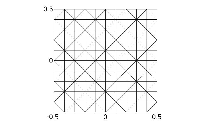
In all our numerical experiments we use the spatial domain $D=(-0.5,0.5)^{2}$ . To partition $D$ we use a uniform triangulation $\mathcal{T}_{h}$ . For a positive integer $n$ , $\mathcal{T}_{1/n}$ denotes the triangulation of $D$ consisting of $2n^{2}$ congruent isosceles triangles with side lengths $1/n,1/n,$ and $\sqrt{2}/n$ . Figure 1 gives the sample triangulation $\mathcal{T}_{1/10}$ .

Refer to caption — Figure 1: Triangulation $\mathcal{T}_{1/10}$

To implement the random noise $\eta$ , we note that $\eta$ only appears in the integration component of our computations. Therefore, we made the choice to implement $\eta$ only at quadrature points of the triangulation. To simulate the random media, we let $\eta$ be an independent random number chosen from a uniform distribution on some closed interval at each quadrature point. Figure 2 shows an example of such random media.

6.1 MCIP-DG with multi-modes expansion compared to classical MCIP-DG

The goal of this subsection is to verify the accuracy and efficiency of the proposed MCIP-DG with the multi-modes expansion. As a benchmark we compare this method to the classical MCIP-DG (i.e. without utilizing the multi-modes expansion). Throughout this section $\tilde{\Psi}^{h}$ is used to denote the computed approximation to $\mathbb{E}(u)$ using the classical MCIP-DG.

In this subsection we set $f=1$ , $k=5$ , $1/h=50$ , $M=1000$ , and $\varepsilon=1/(k+1)$ . Here $\varepsilon$ is chosen with the intent of satisfying the constraint set by the convergence theory in the preceding section. $\eta$ is sampled as described above from a uniform distribution on the interval $[0,1]$ . $\Psi^{h}_{N}$ is computed for $N=1,2,3,4,5$ .

In our first test we compute $\|\Psi^{h}_{N}-\tilde{\Psi}^{h}\|_{L^{2}(D)}$ . The results are displayed in Figure 3. As expected, we find that the difference between $\Psi^{h}_{N}$ and $\tilde{\Psi}^{h}$ is very small. We also observe that we are benefited more by the first couple modes while the help from the later modes is relatively small.

To test the efficiency of our MCIP-DG method with multi-modes expansion, we compare the CPU time for computing $\Psi^{h}_{N}$ and $\tilde{\Psi}^{h}$ . Both methods are implemented on the same computer using Matlab. Matlab’s built-in LU factorization is called to solve the linear systems. The results of this test are shown in Table 1. As expected, we find that the use of the multi-modes expansion improves the CPU time for the computation considerably. In fact, the table shows that this improvement is an order of magnitude. Also, as expected, as the number of modes used is increased the CPU time increases in a linear fashion.

Approximation	CPU Time (s)
$\tilde{\Psi}^{h}$	$3.4954\times 10^{5}$
$\Psi^{h}_{1}$	$1.0198\times 10^{4}$
$\Psi^{h}_{2}$	$2.0307\times 10^{4}$
$\Psi^{h}_{3}$	$3.0037\times 10^{4}$
$\Psi^{h}_{4}$	$3.9589\times 10^{4}$
$\Psi^{h}_{5}$	$4.9011\times 10^{4}$

Table 1: CPU times required to compute the MCIP-DG multi-modes approximation

\Psi^{h}_{N}

and classical MCIP-DG approximation

\tilde{\Psi}^{h}

6.2 More numerical tests

The goal of this subsection is to demonstrate the approximations obtained by our MCIP-DG method with multi-modes expansion using different magnitudes of parameter $\varepsilon$ and different magnitudes of the random noise $\eta$ . We only consider the case $0<\varepsilon<1$ in order to legitimize the series expansion $u^{\varepsilon}$ . With this in mind, we then increase the magnitude of $\eta$ to simulate examples with large noise. Similar to the numerical experiments from [7], we choose the function $f=\sin\big(k\alpha(\omega,\cdot)r\big)/r$ , where $r$ is the radial distance from the origin and $\alpha(\omega,\cdot)$ is implemented as described in the beginning of this section. Since our intention is to observe what happens as we vary $\varepsilon$ and $\eta$ , we fix $k=50$ , $h=1/100$ , and $M=1000$ .

In Figures 4 and 5, we set $\varepsilon=0.02$ and $|\eta|\leq 1$ with the intent of observing the constraints set in the convergence theory from the preceding section. In Figure 4 we present plots of the magnitude of the computed mean ${\rm Re}\big(\Psi^{h}_{3}\big)$ and a computed sample ${\rm Re}\big(U^{h}_{3}\big)$ , respectively, over the whole domain $D$ . Figure 5 gives the plots of a cross section of the computed mean ${\rm Re}\big(\Psi^{h}_{3}\big)$ and a computed sample ${\rm Re}\big(U^{h}_{3}\big)$ , respectively, over the line $y=x$ . In this first example we observe that the computed sample does not differ greatly from the computed mean because $\varepsilon$ is very small.

In Figures 6–11, we fix $|\eta|\leq 1$ and increase $\varepsilon$ past the constraint established in the preceding convergence theory. As expected, we see that as $\varepsilon$ increases the computed sample differs more from the computed mean. We also observe that as $\varepsilon$ increases the phase of the wave remains relatively intact but the magnitude of the wave becomes more uniform.

In Table 2 the relative error (measured in the $L^{2}$ -norm) between the multi-modes approximation $\Psi^{h}_{N}$ and the classical Monte Carlo approximation $\Psi^{h}$ is given for $\varepsilon=0.02,0.1,0.5,0.8$ . In this table only three modes (i.e., $N=3$ ) are used. Recall that the convergence theory in this case only holds for $\varepsilon$ on the order of the first value $0.02$ . That being said, we observe that the approximations corresponding to $\varepsilon=0.1$ and $\varepsilon=0.5$ are relatively close to those obtained using the classical Monte Carlo method. Another observation that can be made from Table 2 is that as $\varepsilon$ increases the relative error increases. This is expected from the convergence theory.

Recall that the error predicted in the convergence theory can be bounded by a term with the factor $\varepsilon^{N}$ . Thus for $\varepsilon$ relatively large, one must use more modes to decrease the error. Keeping this in mind, Table 3 records the relative error (measured in the $L^{2}$ -norm) between the multi-modes approximation $\Psi^{h}_{N}$ and the classical Monte Carlo approximation $\Psi^{h}$ is given for $\varepsilon=0.5,0.8$ and $N=4,5,6,7$ . At this point, we observe that the relative error decreases as N increases when $\varepsilon=0.5$ . On the other hand, the relative error increases as $N$ increases when $\varepsilon=0.8$ . From Tables 2 and 3 we observe that multi-modes expansion $\Psi^{h}_{N}$ is relatively accurate (measured against an approximation from the classical Monte Carlo method) even in cases when $\varepsilon$ does not satisfy the constraint set forth in the convergence theory. We also observe that when $\varepsilon$ becomes too large, the multi-modes expansion no longer agrees with the classical Monte Carlo method.

$\varepsilon$	$0.02$	$0.1$	$0.5$	$0.8$
Relative $L^{2}$ Error	$3.0125\times 10^{-4}$	$6.0073\times 10^{-4}$	$0.2865$	$1.6979$

Table 2:

L^{2}

-norm relative error between the multimodes expansion approximation

\Psi^{h}_{3}

and the classical Monte Carlo approximation

\tilde{\Psi}^{h}

$\varepsilon$	$N=4$	$N=5$	$N=6$	$N=7$
$0.5$	$0.2866$	$0.1125$	$0.1137$	$0.0554$
$0.8$	$1.7036$	$1.6713$	$1.6839$	$1.7887$

Table 3:

L^{2}

-norm relative error between the multimodes expansion approximation

\Psi^{h}_{N}

and the classical Monte Carlo approximation

\tilde{\Psi}^{h}

In Figures 12–19, we fix $\varepsilon=0.9$ and increase the magnitude of $\eta$ . We observe that as the magnitude of random noise increases the difference between computed sample and computed mean increases. We also observe that the phase of the computed wave remains intact until the random noise becomes too large (see Figures 18 and 19). At this point we believe that increasing the number of samples is necessary in order to capture the mean of the large noise.

Acknowledgments. This project was initiated while both the first and second authors were long-term visitors (as a new direction professor and a postdoc, respectively) of IMA at University of Minnesota in the spring of 2013. Both authors are grateful for the financial support and the visiting opportunity provided by IMA.

References

[1] I. Babuška, F. Nobile and R. Tempone. A stochastic collocation method for elliptic partial differential equations with random input data. SIAM Rev., 52:317–355, 2010.
[2] I. Babuška, R. Tempone and G. E. Zouraris. Galerkin finite element approximations of stochastic elliptic partial differential equations. SIAM J. Numer. Anal., 42:800–825, 2004.
[3] R. Caflisch, Monte Carlo and quasi-Monte Carlo methods. Acta Numerica, 7:1–49, 1998.
[4] P. Cummings and X. Feng. Sharp regularity coefficient estimates for complex-valued acoustic and elastic Helmholtz equations. M³AS, 16:139–160, 2006.
[5] M. Eiermann, O. Ernst, and E. Ullmann, Computational aspects of the stochastic finite element method. Proceedings of ALGORITMY, 1-10, 2005.
[6] B. Engquist and A. Majda. Radiation boundary conditions for acoustic and elastic wave calculations. Comm. Pure Appl. Math., 32(3):314–358, 1979.
[7] X. Feng and H. Wu. Discontinuous Galerkin methods for the Helmholtz equation with large wave numbers. SIAM J. Numer. Anal., 47:2872–2896, 2009.
[8] X. Feng and H. Wu. $hp$ -Discontinuous Galerkin methods for the Helmholtz equation with large wave numbers. Math. Comp., 80:1997–2024, 2011.
[9] J. Fouque, J. Garnier, G. Papanicolaou and K. Solna, Wave Propagation and Time Reversal in Randomly Layered Media. Stochastic Modeling and Applied Probability, Vol. 56, Springer, 2007.
[10] O. Ernst and M. Gander. Why it is difficult to solve Helmholtz problems with classical iterative methods? in Numerical Analysis of Multiscale Problems, I. Graham, T. Hou, O. Lakkis and R. Scheichl, Editors, pp. 325-363, Springer Verlag, 2012.
[11] D. Gilbarg, N. S. Trudinger. Elliptic Partial Differential Equations of Second Order, Classics in Mathematics. Springer-Verlag, Berlin, 2001, reprint of the 1998 edition.
[12] A. Ishimaru, Wave Propagation and Scattering in Random Media. IEEE Press, New York, 1997.
[13] R. Leis, Initial-Boundary Value Problems in Mathematical Physics. Tübner, 1986.
[14] K. Liu and B. Rivière. Discontinuous Galerkin methods for elliptic partial differential equations with random coefficients. Int. J. Computer Math., DOI: 10.1080/00207160.2013.784280.
[15] L. Roman and M. Sarkis, Stochastic Galerkin method for elliptic SPDEs: A white noise approach, Discret. Contin. Dyn. S., 6:941-955, 2006.
[16] D. Xiu and G. Karniadakis, The Wiener-Askey polynomial chaos for stochastic differential equations. SIAM J. Sci. Comput., 24:619-644, 2002.

(9)	$\displaystyle\mathbb{E}(\left\\|\nabla u\right\\|_{L^{2}(D)}^{2})$	$\displaystyle\leq\Bigl(k^{2}(1+\varepsilon)^{2}+\delta_{1}\Bigr)\mathbb{E}(\left\\|u\right\\|_{L^{2}(D)}^{2})$
	$\displaystyle\qquad+\left(\frac{\delta_{1}}{2k^{2}(1-\varepsilon)^{2}}+\frac{1}{2\delta_{1}}\right)\left(\mathbb{E}(\left\\|f\right\\|_{L^{2}(D)}^{2})+\mathbb{E}(\left\\|g\right\\|_{L^{2}(\partial D)}^{2})\right),$
(10)	$\displaystyle\mathbb{E}(\left\\|u\right\\|_{L^{2}(\partial D)}^{2})$	$\displaystyle\leq\frac{\delta_{2}}{k(1-\varepsilon)}\mathbb{E}(\left\\|u\right\\|_{L^{2}(D)}^{2})+\frac{1}{\delta_{2}k(1-\varepsilon)}\mathbb{E}(\left\\|f\right\\|_{L^{2}(D)}^{2})$
	$\displaystyle\qquad+\frac{1}{k^{2}(1-\varepsilon)^{2}}\mathbb{E}(\left\\|g\right\\|_{L^{2}(\partial D)}^{2}).$

	$\displaystyle\nabla\cdot(x\|\nabla u\|^{2})$	$\displaystyle=d\|\nabla u\|^{2}+x\cdot\nabla(\|\nabla u\|^{2}),$
	$\displaystyle x\cdot\nabla(\|\nabla u\|^{2})$	$\displaystyle=2{\rm Re}\Bigl(\nabla\cdot(\nabla u(\overline{x\cdot\nabla u}))-\Delta u(\overline{x\cdot\nabla u})\Bigr)-2\|\nabla u\|^{2}$
		$\displaystyle=2{\rm Re}\bigl(\,\nabla u\cdot\overline{\nabla(x\cdot\nabla u)}\,\bigr)-2\|\nabla u\|^{2}.$

	$\displaystyle\frac{dk^{2}}{2}\mathbb{E}(\left\\|u\right\\|_{L^{2}(D)}^{2})$	$\displaystyle\leq\frac{d-2}{2}\mathbb{E}(\left\\|\nabla u\right\\|_{L^{2}(D)}^{2})+k^{2}\varepsilon R(2+\varepsilon)\Bigl(\frac{1}{2\delta_{1}}\mathbb{E}(\left\\|u\right\\|_{L^{2}(D)}^{2})$
		$\displaystyle\qquad+\frac{\delta_{1}}{2}\mathbb{E}(\left\\|\nabla u\right\\|_{L^{2}(D)}^{2})\Bigr)+\frac{R}{2\delta_{2}}\mathbb{E}(\left\\|f\right\\|_{L^{2}(D)}^{2})+\frac{R\delta_{2}}{2}\mathbb{E}(\left\\|\nabla u\right\\|_{L^{2}(D)}^{2})$
		$\displaystyle\qquad+\frac{R}{2\delta_{3}}\mathbb{E}(\left\\|g\right\\|_{L^{2}(\partial D)}^{2})+\frac{R\delta_{3}}{2}\mathbb{E}(\left\\|\nabla u\right\\|_{L^{2}(\partial D)}^{2})$
		$\displaystyle\qquad+\frac{kR}{\delta_{4}}\mathbb{E}(\left\\|u\right\\|_{L^{2}(\partial D)}^{2})+kR\delta_{4}\mathbb{E}(\left\\|\nabla u\right\\|_{L^{2}(\partial D)}^{2})$
		$\displaystyle\qquad-\frac{c_{0}}{2}\mathbb{E}\bigl(\left\\|\nabla u\right\\|_{L^{2}(\partial D)}^{2}\bigr)+\frac{k^{2}R}{2}\mathbb{E}\bigl(\left\\|u\right\\|_{L^{2}(\partial D)}^{2}\bigr).$

		$\displaystyle\frac{dk^{2}}{2}\mathbb{E}(\left\\|u\right\\|_{L^{2}(D)}^{2})\leq\Bigl(\frac{d-2}{2}+\frac{k^{2}R\gamma\delta_{1}}{2}+\frac{R\delta_{2}}{2}\Bigr)\mathbb{E}(\left\\|\nabla u\right\\|_{L^{2}(D)}^{2})+\frac{k^{2}R\gamma}{2\delta_{1}}\mathbb{E}(\left\\|u\right\\|_{L^{2}(D)}^{2})$
		$\displaystyle\qquad\qquad+\Bigl(\frac{8k^{2}R^{2}}{c_{0}}+\frac{k^{2}R}{2}\Bigr)\mathbb{E}(\left\\|u\right\\|_{L^{2}(\partial D)}^{2})-\frac{c_{0}}{4}\mathbb{E}\bigl(\left\\|\nabla u\right\\|_{L^{2}(\partial D)}^{2}\bigr)$
		$\displaystyle\qquad\qquad+\frac{R}{2\delta_{2}}\mathbb{E}(\left\\|f\right\\|_{L^{2}(D)}^{2})+\frac{2R^{2}}{c_{0}}\mathbb{E}(\left\\|g\right\\|_{L^{2}(\partial D)}^{2})$
		$\displaystyle\qquad\leq\Bigl(\frac{d-2}{2}+\frac{k^{2}R\gamma\delta_{1}}{2}+\frac{R\delta_{2}}{2}\Bigr)\left(k^{2}(1+\gamma)+\delta_{5}\right)\mathbb{E}(\left\\|u\right\\|_{L^{2}(D)}^{2})$
		$\displaystyle\qquad\qquad+\Bigl(\frac{d-2}{2}+\frac{k^{2}R\gamma\delta_{1}}{2}+\frac{R\delta_{2}}{2}\Bigr)\Bigl(\frac{2\delta_{5}}{k^{2}}+\frac{1}{2\delta_{5}}\Bigr)\left(\mathbb{E}(\left\\|f\right\\|_{L^{2}(D)}^{2})+\mathbb{E}(\left\\|g\right\\|_{L^{2}(\partial D)}^{2})\right)$
		$\displaystyle\qquad\qquad+\Bigl(\frac{8k^{2}R^{2}}{c_{0}}+\frac{k^{2}R}{2}\Bigr)\Bigl(2\delta_{6}\mathbb{E}(\left\\|u\right\\|_{L^{2}(D)}^{2})+\frac{2}{k^{2}\delta_{6}}\mathbb{E}(\left\\|f\right\\|_{L^{2}(D)}^{2})+\frac{4}{k^{2}}\mathbb{E}(\left\\|g\right\\|_{L^{2}(\partial D)}^{2})\Bigr)$
		$\displaystyle\qquad\qquad+\frac{k^{2}R\gamma}{2\delta_{1}}\mathbb{E}(\left\\|u\right\\|_{L^{2}(D)}^{2})+\frac{R}{2\delta_{2}}\mathbb{E}(\left\\|f\right\\|_{L^{2}(D)}^{2})+\frac{2R^{2}}{c_{0}}\mathbb{E}(\left\\|g\right\\|_{L^{2}(\partial D)}^{2})-\frac{c_{0}}{4}\mathbb{E}\bigl(\left\\|\nabla u\right\\|_{L^{2}(\partial D)}^{2}\bigr),$

	$\displaystyle\mathbb{E}(\left\\|u\right\\|_{H^{1}(D)}^{2})$	$\displaystyle=\mathbb{E}(\left\\|u\right\\|_{L^{2}(D)}^{2})+\mathbb{E}(\left\\|\nabla u\right\\|_{L^{2}(D)}^{2})$
		$\displaystyle\leq\frac{C}{k^{2}}\Bigl(1+\frac{1}{k^{2}}\Bigr)\Bigl(\mathbb{E}(\left\\|f\right\\|_{L^{2}(D)}^{2})+\mathbb{E}(\left\\|g\right\\|_{L^{2}(\partial D)}^{2})\Bigr)$
		$\displaystyle\qquad\qquad+\left(k^{2}(1+\varepsilon)^{4}+k^{2}\right)\mathbb{E}(\left\\|u\right\\|_{L^{2}(D)}^{2})$
		$\displaystyle\qquad\qquad+\Bigl(1+\frac{1}{2k^{2}}\Bigr)\Bigl(\mathbb{E}(\left\\|f\right\\|_{L^{2}(D)}^{2})+\mathbb{E}(\left\\|g\right\\|_{L^{2}(\partial D)}^{2})\Bigr)$
		$\displaystyle\leq C\Bigl(1+\frac{1}{k^{2}}\Bigr)^{2}\Bigl(\mathbb{E}(\left\\|f\right\\|_{L^{2}(D)}^{2})+\mathbb{E}(\left\\|g\right\\|_{L^{2}(\partial D)}^{2})\Bigr).$

An efficient numerical method for acoustic wave scattering in random media

Abstract

keywords

AMS

1 Introduction

2 PDE analysis

2.1 Preliminaries

Definition 1.

Remark 2.1.

2.2 Wave-number-explicit solution estimates

Lemma 2.

Proof.

Lemma 3.

Proof.

Remark 2.2.

Theorem 4.

Proof.

Remark 2.3.

Theorem 5.

Proof.

Remark 2.4.

3 Multi-modes representation of the solution and its finite modes approximations

Theorem 6.

Proof.

Theorem 7.

Proof.

Theorem 8.

Proof.

4 Monte Carlo discontinuous Galerkin approximations of the mode functions {𝐮𝐧}\mathbf{\{u_{n}\}}

4.1 DG notations

4.2 IP-DG method for deterministic Helmholtz problem

Remark 4.1.

Theorem 9.

Corollary 10.

Theorem 11.

Remark 4.2.

4.3 MCIP-DG method for approximating 𝔼⁡(𝐮𝐧)\mathbf{\mathbb{E}(u_{n})} for 𝐧≥𝟎\mathbf{n\geq 0}

Lemma 12.

Lemma 13.

Proof.

Theorem 14.

Remark 4.3.

5 The overall numerical procedure

5.1 The numerical algorithm, linear solver and computational complexity

5.2 Convergence analysis

Lemma 15.

Lemma 16.

Proof.

Theorem 17.

Theorem 18.

Proof.

Theorem 19.

6 Numerical experiments

6.1 MCIP-DG with multi-modes expansion compared to classical MCIP-DG

6.2 More numerical tests

References

4 Monte Carlo discontinuous Galerkin approximations of the mode functions $\mathbf{\{u_{n}\}}$

4.3 MCIP-DG method for approximating $\mathbf{\mathbb{E}(u_{n})}$ for $\mathbf{n\geq 0}$