Electroweak precision measurements in supersymmetric models with a lepton number
Abstract
As experimental constraints on the parameter space of the MSSM and close variations thereof become stronger, the motivation to explore supersymmetric models that challenge some of the standard assumptions of the MSSM also become stronger. For example, models where the gauginos are Dirac instead of Majorana have recently received more attention. Beside allowing for a supersoft SUSY breaking mechanism where the gauginos only provide finite threshold corrections to scalar masses, the cross section for the production of a squark pairs is reduced. In addition, Dirac gauginos can be used to build models that possess a symmetry. This symmetry can then be identified with a lepton number, leading to models that are quite different from conventional scenarios. The sneutrinos in these models can acquire a vev and give mass to the leptons and the down-type squark. The phenomenology is novel, combining signatures that are typical of R-parity violating scenarios with signatures arising from leptoquarks. Correspondingly the constraints from electroweak precision data are also different. In these models, one of the leptons mixes with gauginos and superpotential Yukawa couplings can contribute to EWPM at tree level. In addition, lepton universality is broken. In this paper we adapt the operators analysis of Han and Skiba [1] to include the relevant violation of lepton universality, and do a global fit of the model to electroweak precision data, including all relevant tree-level and loop-level effects. We obtain bounds on the vev of the sneutrino and on the superpotential couplings of the model.
1 Introduction
Supersymmetry (SUSY) as a solution to the hierarchy problem is now, after two years of LHC data, under severe tension. This has motivated the exploration of a wide range of supersymmetric models, relaxing several assumptions built into the conventional Minimal Supersymmetric Standard Model (MSSM). One possibility put forward is to have models where the gauginos are Dirac instead of Majorana [2, 3, 4, 5, 6, 7, 8, 9, 10, 11, 12, 13, 14, 15, 16, 17, 18]. While this requires an enlarged field content, it could also be less constrained by LHC data due to the fact that gluinos could be heavier with the same fine-tuning if SUSY breaking is supersoft [5] and that squark pair production has a smaller cross-section when the gluinos are Dirac [19, 20]. Also, with Dirac gauginos, one can impose an approximate symmetry on the model and this was shown to alleviate flavor constraints on the squark mass matrices [7]. Furthermore, the symmetry can be identified with a lepton number [21, 22, 23] (see [24, 25, 26, 27] for earlier work) . This allows for reduction of the Higgs sector of the model (which would otherwise need four doublets [7]), by allowing the sneutrino to get a vacuum expectation value (vev) and play the role of the down-type Higgs. In this setup, the constraints on the vev of the sneutrino are much milder than in traditional supersymmetric models because the sneutrino does not carry lepton number and giving it a vev does not introduce unacceptably large neutrino masses. The down-type quarks and the leptons then acquire a mass through -parity violating coupling (where here -parity means the conventional -parity, not the subgroup of the full we are imposing on the model). It is well known that such couplings will lead to deviations to electroweak precision observables (see [28] for a review), and it is the goal of this paper to study more in depth the constraints that electroweak precision observables put on the model. A preliminary study of such constraints was performed in [22, 23], and LHC phenomenology was studied in [29]. In [22, 23], the constraints were estimated by looking at the tree-level effect of the new couplings which were considered in isolation. In this paper, we analyze the constraints more thoroughly by considering loop effects as well and fitting to all relevant electroweak data. We adopt the operator method of [1] to analyze the constraints on the parameter space of the model. However, because our model leads to deviations from flavor universality in the lepton sector, we need to generalize the analysis of [1, 30] to take these effects into account.
2 The Model
In this section, we present a review of the model which was described in details in [22, 23]. In addition to the usual matter chiral superfields, , the model has two doublet chiral superfields:
| (1) |
with hypercharge and respectively, and a set of chiral superfields that are in the adjoint representation of the Standard Model gauge group:
| (2) |
where is an adjoint of color, an adjoint of and a singlet.
The superfield has the same quantum numbers as the down-type Higgs superfield of the MSSM, but we do not use the name as in our model this field does not acquire a vev. Its scalar component is an inert doublet. The adjoint chiral superfields are added to give Dirac masses to gauginos. These masses occur through a superpotential term of the form [5] (shown here for the winos):
| (3) |
where is a real superfield that acts as a spurion with a non-zero term: . In addition to a mass term of the form
| (4) |
the superpotential term above also leads, once the classical equations of motion are solved, to a non-standard expression for :
| (5) | ||||
where and are respectively the generators of the two and three dimensional representations of .
As mentioned above, it is the sneutrino and not which acquires a vev providing masses to down-type fermions in this model. Therefore, the part of the superpotential responsible for the masses of the standard model particles will be of the form:
| (6) |
The subscript on the lepton chiral superfield denotes the flavor of the sneutrino that acquires a vev. The two other lepton flavors are labeled and . This superpotential is invariant under a symmetry where the superfields and have R-charge 0, while have -charge 1 and and have -charge 2. The and terms are the standard R-parity violating terms, which in the literature have coefficients called and respectively. Here they are the Yukawa couplings. We also include in the superpotential terms of the form:
| (7) |
where , which respect all the symmetries of the model and can contribute to raising the Higgs mass at loop level [31]. We take the soft SUSY breaking terms, in addition to the Dirac gaugino masses (see eq. (4)), to be:
| (8) |
where the sum runs over all scalars. We see here that because doesn’t have a -term, it will not get a vev, as long as its mass squared is positive. On the other hand, due to the presence of the term, the sneutrino will acquire one.
3 Contributions to electroweak precision measurements
In this section, the corrections to the electroweak precision measurements (EWPM) coming from the new physics are presented. Since all new particles are experimentally constrained to be rather heavy, their contributions can be parametrized to a good approximation in terms of dimension six effective operators respecting the Standard Model gauge symmetries. We use the same basis as in [1] but do not assume a full flavor symmetry, which is not present in our model since only one flavour of sneutrino gets a vev. However, we do not consider operators that lead to FCNC in the lepton or quark sector as those would be much more strongly constrained, and can be avoided in our model by appropriate assumptions on the flavour sector. The operators containing only gauge bosons and Higgs particles are [1]
| (9) |
The four-fermion operators that are relevant to EWPM, where we explicitly show the lepton flavor indices, are [1]
| (10) | ||||||
The operators that modify the coupling between fermions and gauge bosons are [1] 11 1 Because this is a two Higgs doublets model, one could also write operators with the second doublet. However, the effects of those on precision observables can be absorbed in the operators of (11). :
| (11) | ||||||
Finally, there is one operator affecting only gauge boson self-interactions [1]
| (12) |
The total effective Lagrangian is therefore the sum of the Lagrangian of the SM and a linear combination of the different dimension six operators:
| (13) |
where represent the operators, and are coefficients with dimension of inverse mass squared.
In the following sections, we present the contributions to the different operators. We first compute the coefficients of operators related to oblique corrections. Then, the four-fermion operators coming from scalar exchange and box diagrams are presented. Operators that modify gauge boson vertices coming from loop diagrams and mixing are shown. Finally, the contributions to the operator are discussed.
3.1 Oblique parameters
A standard and convenient way of parametrizing deviations to EWPM is through the so-called oblique parameters [32, 33], which are defined to be modifications to two point functions of the electroweak gauge bosons. Coefficients of some of the higher dimensional operators mentioned above can in turn be written as a function of the oblique parameters. In this section, we present these relationships and the computation of the oblique parameters in our model due to a vev of the third component of the triplet and loops of scalars and fermions. We use the definitions of [34] for the definitions of the oblique parameters , , and (see also [35]):
| (14) |
Following [34], we compute loop-level contributions to these parameters by considering diagrams of the form shown in figure 1, where the vevs are treated as perturbations. The first two parameters are linked to and by
| (15) |
The two others are related to operators which are not listed in (9):
| (16) |
However, using the equations of motions, these operators can be written in terms of the operators shown in (9), (10) and (11) (plus additional operators that do not contribute to EWPM). Only eliminating leads to additional contribution to the operators of (9). More precisely it gives rise to an operator, amongst others, of the form
| (17) |
This operator can then be related to and terms irrelevant to EWPM. The net effect on due to is:
| (18) |
In practice, this contribution is overshadowed by the term. The operator can also be eliminated using the equations of motion, but does not give a contribution to the operators of (9).

3.1.1 Vev of
In general, the field will acquires a vev of the form
| (19) |
where and and are the vev of the neutral component of and respectively. This will give a tree-level contribution to through a correction to the charged boson mass:
| (20) |
For a light enough scalar triplet, this contributions dominates the parameter. The singlet also acquires a small vev. However, it is not a direct contribution and its effect is therefore much smaller and can be ignored.
3.1.2 Scalars
Loops of scalars will contribute to the oblique parameters. The relevant couplings come from (5), (6) and (7). The first term of each line of (5) are present in the MSSM and lead to contributions similar to those presented in [34].
For sfermions, the results of [34] apply almost directly. The only difference is that, as provides mass to the down type quarks and leptons, we include its scalar contributions in the Higgs sector. This has the advantage of making expressions simpler and easier to compare. The sfermions contributions are
| (21) | ||||
where and is given in [34]:
| (22) |
The scalar field, despite not acquiring a vev, still contributes to the oblique parameters. For and , its contributions are similar to those of and and can be read from (21) directly. For and , the presence of (7) changes the result. The parameters are
| (23) | ||||
where . The Higgs sector (including the scalar part of ) gives contributions to , and that can once again be obtained by using the results of [34] almost directly. In terms of , these contributions are
| (24) | ||||
The presence of the scalar components of the singlet and triplet do not lead to any contribution to and by themselves, but only a contribution to :
| (25) |
where . The contribution to from diagrams with higgs, triplet and singlets is however more difficult to compute using insertions of the Higgs vev because of the mixing between the Higgs and the triplet. Therefore, we compute these contributions by numerically diagonalizing the scalar mass matrix.
3.1.3 Higgsinos and gauginos
The fit constrains the value of to a region of phase space where it is much smaller than . As such, the contributions to the oblique parameters containing only powers of dominate and are presented here. The contributions containing powers of were also included in the numerical fit. With the exception of the contributions coming from couplings and , the diagrams with binos are usually smaller by an order of magnitude or so and are not presented for simplicity, but were included in the fit. The dominant terms in the limit of and small are
| (26) | ||||
where . The oblique parameters containing and are included but not presented here as the expressions are rather long. The contribution to the parameter is in fact the dominant term in setting limits on and for massive enough scalar gauge particles.
3.2 Four-fermion operators
There are many contributions to the four-fermion operators. These can come from the operators (16) associated to and once the equation of motion are used, from scalar exchange and from box diagrams. The contributions proportional to and are given by:
| (27) |
where and stand for the different combinations of fields possible. The family indices are suppressed because they are the same for every combination, as is expected from the fact that the oblique parameters are universal.
The tree-level scalar exchange contributions come from the exchange of sfermions between leptons or down quarks. The scalars are integrated out and the diagrams are rewritten using the Fiertz rearrangement formulas. In practice, most of them have a negligible effect on the fit as they involve small Yukawa couplings. The only important ones are those which contribute to the observables and [36]. They are
| (28) |
where and are the Yukawa coupling of leptons and respectively. Note that being proportional to lepton Yukawa, the contributions to these operators increases as is lowered and will lead to a lower (upper) bound on ().
Box diagrams like those of [2] are also accounted for with four-fermion operators, though the expressions are too long to be included here. In the case of diagrams including an exchange of sleptons , the limit of large is also taken, as it is strongly overshadowed by mixing effects anyway.

3.3 Vertex modifying operators
The operators of (11) receive contributions from lepton mixing, oblique parameters ( and ) and loop diagrams. Because the left-handed parts of the leptons of family mix with superpartners of different gauge charges, the interactions between the gauge bosons and the physical leptons are modified. The result is readily obtained by replacing the leptons of family and the relevant superpartners by their equivalent combinations of mass eigenstates in the gauge boson vertex interaction terms. This can be summarized in terms of effective operators with coefficients
| (29) |
The right handed part of the lepton of family mixes as well, but this effects is suppressed with respect to left-handed mixing by a factor of and is therefore ignored. These operators lead to deviations of the coupling of the lepton of flavour to the SM gauge bosons, and will lead to an upper (lower) bound on ().
The contribution from oblique parameters that arise once and are eliminated are given by
| (30) |
Once again, the family indices are suppressed because they are the same for every generation.
Finally, loop-level diagrams of the type shown in figure 3 also lead to corrections to the gauge boson fermion vertices. They appear in the four possible ways shown. We can parametrize their effects in terms of 22 2 To avoid a possible sign confusion, we mention that covariant derivatives are taken with a sign. For example, .
| (31) | ||||
It can be shown that these quantities are related by . Using this relation, the diagrams can be accounted for by using the operators of (11). This leads to coefficients of
| (32) |
The same equations also apply to quarks. The diagrams containing Yukawa coupling are neglected as these are considerably smaller. The limit of large is also taken when an internal slepton is present.

3.4 Loop contributions to
The contributions to the operator arise at loop level. As this operator leads only to triple gauge boson interactions, it is very poorly constrained and its effect on the fit is negligible. It is therefore not included.
4 Method and results
| Standard Notation | Measurement | Reference | |
| Atomic parity | Weak charge in Cs | [37] | |
| violation | Weak charge in Tl | [38, 39] | |
| DIS | , | -nucleon scattering from NuTeV | [40] |
| -nucleon scattering from CDHS and CHARM | [41, 42] | ||
| -nucleon scattering from CCFR | [43] | ||
| , | - scattering from CHARM II | [44] | |
| Z-pole | Total Z width | [45] | |
| hadronic cross section at Z pole | [45] | ||
| Ratios of decay rates | [45] | ||
| Forward-backward asymmetries | [45] | ||
| Polarized asymmetries | [45] | ||
| Fermion pair | Total cross section for | [45] | |
| production at | Forward-backward asymmetries for | [45] | |
| LEP2 | Differential cross section for | [46] | |
| pair | Differential cross section for | [47] | |
| mass | [45, 48] | ||
| Ratio of lepton | Ratio of decay rate of to on to | [36] | |
| decay rate | Ratio of decay rate of to on to | [36] |
The coefficients of the different operators are constrained using the observables of table [1]. They are those of [1] with a few minor differences. The observable is not used because it assumes lepton universality which is not the case with the model. The ratios of decay rates and [36] are included, as they affect strongly the lower limit on . These two observables would be unaffected if symmetry was assumed.
The correction to each observable is calculated to linear order in the coefficients of the higher dimensional operators and this is then used to calculate the distribution. Each coefficient is then replaced by its expression in terms of the parameters of the theory. It is then possible to set a number of parameters and do a fit on the remaining ones. These parameters are then constrained inside a region of phase space with a given confidence level.
| Figure | , | , | ||||||
|---|---|---|---|---|---|---|---|---|
| 200 | ||||||||
| 4(a) | 500 | 700 | 400 | 1000 | 700 | Variable | ||
| 600 | ||||||||
| 200 | ||||||||
| 4(b) | 500 | 700 | 400 | 1000 | 1000 | Variable | ||
| 600 | ||||||||
| 5(a) | 500 | 700 | 400 | 1000 | 700 | 0 | ||
| 5(b) | 500 | 700 | 400 | 1000 | 1000 | 0 | ||
| 500 | ||||||||
| 6(a), 6(b) | NA | 500 | 700 | 400 | 1000 | 700 | 0 | NA |
| 1000 |
For the set of masses that we consider (shown in table [2]), we find that fits of our model to the data are roughly as good as the Standard Model fit. As mentioned above, the vev for the triplet is potentially dangerous so we restricted the mass parameter of the scalar triplet to be 1 TeV. The result of the per degree of freedom for different choices of parameters is also shown in table [2]. The allowed region of parameter space, in the // space consists of a roughly cylindrical region whose flat sides are parallel to the plane. The parameter has contributions that scale as and and is the dominant factor in determining the shape of the allowed region for and . Figure [4] shows this region of allowed phase space in the plane for different combinations of masses which can be found in table [2]. We show the 95.45 confidence level exclusion only as the lines of confidence level of 68.27 and 99.76 are very close to those of 95.45 and provide little new information. We see that there are strong bounds on those parameters, with the allowed region becoming larger as is increased as it set the scale of and the masses of the fermions which give the largest loop contributions to . Overall, we see that and cannot take values much greater than one irrespective of the masses of the superpartner or the choice of generation for the lepton . This has important consequences for radiative corrections to the Higgs mass in this model [31].
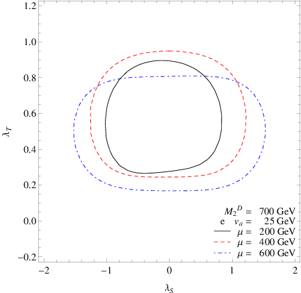
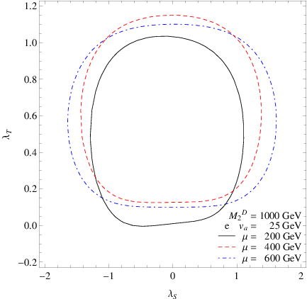
As explained before, contributions (28) and (29) lead to a two-sided bound on which is constrained to be rather small, though the exact range depends considerably on the choice of masses and the generation of the lepton . This is illustrated in figure [5] which shows the allowed region in the plane. Again, the upper bound on is relaxed as is increased and can reach a value where for and GeV. The lower bound on primarily depends on the mass of the sfermions which are not varied in the figures.
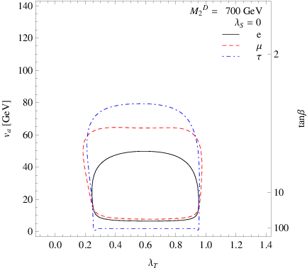
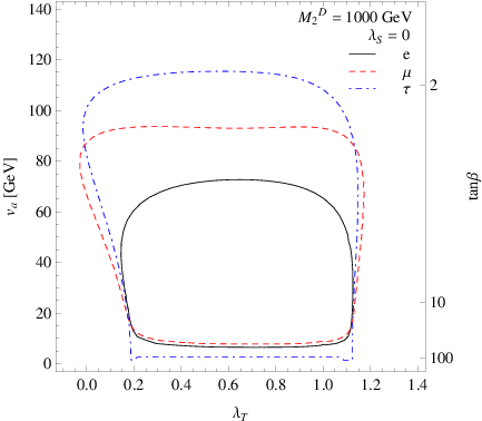
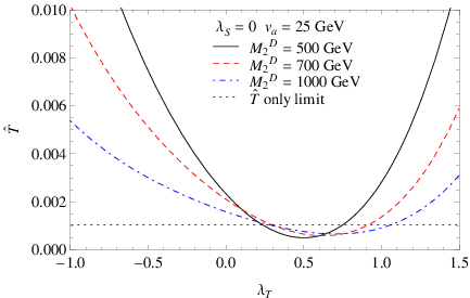
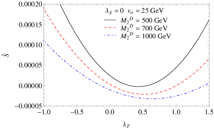
In figure [6], we show the and parameters as a function of . We see that the parameter is very small while the parameter can become sizable and drives the limit on .
Overall, as one would expect, increasing the various mass parameters will relax the various bounds. The situation for is however slightly more involved as increasing will increase (see equation (19)) which can then be taken back to an acceptable value by constraining to be close to .
5 Conclusions
In this paper, we have studied the bounds that electroweak precision measurements put on a supersymmetric model where a lepton number is identified with a symmetry and one of the sneutrino gets a vev and is responsible for giving masses to the down-type quarks and the leptons. Deviations from Standard Model predictions for electroweak precision observables come from various sources: mixing of one of the lepton flavor with the gauginos, a vev for an scalar triplet, tree level exchange of sfermions through the Yukawa couplings and loops of superpartner. To bound the parameter space of this model we used the higher dimensional operators method developed in [1], extended to include the relevant breaking of lepton universality. Our results are illustrated in figure [4] and [5]. The first figure shows that , the superpotential coupling between the Higgs doublets and the triplet, is prevented from taking large value. This coupling also gives a sizable radiative contribution to the Higgs mass so this bound has important repercussions [31]. However, note that in this work we remained agnostic about the precise mechanism that gives the Higgs its correct mass. The second figure shows the bounds on the vev of the sneutrino. It cannot be too large as this creates a large mixing between the corresponding lepton and the gaugino, but it also cannot be too small as this implies a large Yukawa coupling, and leads to deviation to and . Nevertheless, a relatively large range is still allowed, with the possibility of having as low as for gauginos with a 1 TeV Dirac mass.
Acknowledgements.
We would like to thank Enrico Bertuzzo, Claudia Frugiuele and Eduardo Pontón for useful discussions. This work was supported in part by the Natural Sciences and Engineering Research Council of Canada (NSERC).References
- (1) Z. Han and W. Skiba, Effective theory analysis of precision electroweak data, Phys.Rev. D71 (2005) 075009, [hep-ph/0412166].
- (2) L. Hall and L. Randall, U(1)-R symmetric supersymmetry, Nucl.Phys. B352 (1991) 289–308.
- (3) L. Randall and N. Rius, The Minimal U(1)-R symmetric model revisited, Phys.Lett. B286 (1992) 299–306.
- (4) A. E. Nelson, N. Rius, V. Sanz, and M. Unsal, The Minimal supersymmetric model without a mu term, JHEP 0208 (2002) 039, [hep-ph/0206102].
- (5) P. J. Fox, A. E. Nelson, and N. Weiner, Dirac gaugino masses and supersoft supersymmetry breaking, JHEP 0208 (2002) 035, [hep-ph/0206096].
- (6) Z. Chacko, P. J. Fox, and H. Murayama, Localized supersoft supersymmetry breaking, Nucl.Phys. B706 (2005) 53–70, [hep-ph/0406142].
- (7) G. D. Kribs, E. Poppitz, and N. Weiner, Flavor in supersymmetry with an extended R-symmetry, Phys.Rev. D78 (2008) 055010, [arXiv:0712.2039].
- (8) K. Benakli and M. Goodsell, Dirac Gauginos in General Gauge Mediation, Nucl.Phys. B816 (2009) 185–203, [arXiv:0811.4409].
- (9) S. Choi, M. Drees, A. Freitas, and P. Zerwas, Testing the Majorana Nature of Gluinos and Neutralinos, Phys.Rev. D78 (2008) 095007, [arXiv:0808.2410].
- (10) G. D. Kribs, T. Okui, and T. S. Roy, Viable Gravity-Mediated Supersymmetry Breaking, Phys.Rev. D82 (2010) 115010, [arXiv:1008.1798].
- (11) S. Abel and M. Goodsell, Easy Dirac Gauginos, JHEP 1106 (2011) 064, [arXiv:1102.0014].
- (12) R. Davies, J. March-Russell, and M. McCullough, A Supersymmetric One Higgs Doublet Model, JHEP 1104 (2011) 108, [arXiv:1103.1647].
- (13) P. Kumar and E. Ponton, Electroweak Baryogenesis and Dark Matter with an approximate R-symmetry, JHEP 1111 (2011) 037, [arXiv:1107.1719].
- (14) E. Bertuzzo and C. Frugiuele, Fitting Neutrino Physics with a Lepton Number, JHEP 1205 (2012) 100, [arXiv:1203.5340].
- (15) H. Itoyama and N. Maru, D-term Dynamical Supersymmetry Breaking Generating Split N=2 Gaugino Masses of Mixed Majorana-Dirac Type, Int.J.Mod.Phys. A27 (2012) 1250159, [arXiv:1109.2276].
- (16) H. Itoyama and N. Maru, D-term Triggered Dynamical Supersymmetry Breaking, Phys. Rev. D88 (2013) 025012, [arXiv:1301.7548].
- (17) H. Itoyama and N. Maru, 126 GeV Higgs Boson Associated with D-term Triggered Dynamical Supersymmetry Breaking, arXiv:1312.4157.
- (18) S. Charkraborty and S. Roy, Higgs boson mass, neutrino masses and mixing and keV dark matter in an U(1)R− lepton number model, JHEP 1401 (2014) 101, [arXiv:1309.6538].
- (19) M. Heikinheimo, M. Kellerstein, and V. Sanz, How Many Supersymmetries?, JHEP 1204 (2012) 043, [arXiv:1111.4322].
- (20) G. D. Kribs and A. Martin, Supersoft Supersymmetry is Super-Safe, Phys.Rev. D85 (2012) 115014, [arXiv:1203.4821].
- (21) T. Gherghetta and A. Pomarol, The Standard model partly supersymmetric, Phys.Rev. D67 (2003) 085018, [hep-ph/0302001].
- (22) C. Frugiuele and T. Gregoire, Making the Sneutrino a Higgs with a Lepton Number, Phys.Rev. D85 (2012) 015016, [arXiv:1107.4634].
- (23) C. Frugiuele, T. Gregoire, P. Kumar, and E. Ponton, ’L=R’ - as the Origin of Leptonic ’RPV’, JHEP 1303 (2013) 156, [arXiv:1210.0541].
- (24) P. Fayet, Supergauge Invariant Extension of the Higgs Mechanism and a Model for the electron and Its Neutrino, Nucl.Phys. B90 (1975) 104–124.
- (25) P. Fayet, Supersymmetry and Weak, Electromagnetic and Strong Interactions, Phys.Lett. B64 (1976) 159.
- (26) P. Fayet, Spontaneously Broken Supersymmetric Theories of Weak, Electromagnetic and Strong Interactions, Phys.Lett. B69 (1977) 489.
- (27) P. Fayet, MASSIVE GLUINOS, Phys.Lett. B78 (1978) 417.
- (28) R. Barbier, C. Berat, M. Besancon, M. Chemtob, A. Deandrea, et al., R-parity violating supersymmetry, Phys.Rept. 420 (2005) 1–202, [hep-ph/0406039].
- (29) C. Frugiuele, T. Gregoire, P. Kumar, and E. Ponton, ’L=R’ – Lepton Number at the LHC, JHEP 1305 (2013) 012, [arXiv:1210.5257].
- (30) Z. Han, Electroweak constraints on effective theories with U(2) x (1) flavor symmetry, Phys.Rev. D73 (2006) 015005, [hep-ph/0510125].
- (31) E. Bertuzzo, C. Frugiuele, T. Grégoire, and E. Pontón, Dirac gauginos, r symmetry and the 125 gev higgs, To appear.
- (32) M. E. Peskin and T. Takeuchi, Estimation of oblique electroweak corrections, Phys.Rev. D46 (1992) 381–409.
- (33) M. E. Peskin and T. Takeuchi, A New constraint on a strongly interacting Higgs sector, Phys.Rev.Lett. 65 (1990) 964–967.
- (34) G. Marandella, C. Schappacher, and A. Strumia, Supersymmetry and precision data after LEP2, Nucl.Phys. B715 (2005) 173–189, [hep-ph/0502095].
- (35) R. Barbieri, A. Pomarol, R. Rattazzi, and A. Strumia, Electroweak symmetry breaking after LEP-1 and LEP-2, Nucl.Phys. B703 (2004) 127–146, [hep-ph/0405040].
- (36) F. Ledroit and G. Sajot, Indirect limits on SUSY violating couplings and , GDR-S-008 (1998).
- (37) C. Wood, S. Bennett, D. Cho, B. Masterson, J. Roberts, et al., Measurement of parity nonconservation and an anapole moment in cesium, Science 275 (1997) 1759–1763.
- (38) P. Vetter, D. Meekhof, P. Majumder, S. Lamoreaux, and E. Fortson, Precise test of electroweak theory from a new measurement of parity nonconservation in atomic thallium, Phys.Rev.Lett. 74 (1995) 2658–2661.
- (39) N. Edwards, S. Phipp, P. Baird, and S. Nakayama, Precise Measurement of Parity Nonconserving Optical Rotation in Atomic Thallium, Phys.Rev.Lett. 74 (1995) 2654–2657.
- (40) NuTeV Collaboration Collaboration, G. Zeller et al., A Precise determination of electroweak parameters in neutrino nucleon scattering, Phys.Rev.Lett. 88 (2002) 091802, [hep-ex/0110059].
- (41) A. Blondel, P. Bockmann, H. Burkhardt, F. Dydak, A. Grant, et al., Electroweak Parameters From a High Statistics Neutrino Nucleon Scattering Experiment, Z.Phys. C45 (1990) 361–379.
- (42) CHARM Collaboration Collaboration, J. Allaby et al., A Precise Determination of the Electroweak Mixing Angle from Semileptonic Neutrino Scattering, Phys.Lett. B177 (1986) 446.
- (43) CCFR Collaboration, E744 Collaboration, E770 Collaboration Collaboration, K. S. McFarland et al., A Precision measurement of electroweak parameters in neutrino - nucleon scattering, Eur.Phys.J. C1 (1998) 509–513, [hep-ex/9701010].
- (44) CHARM-II Collaboration Collaboration, P. Vilain et al., Precision measurement of electroweak parameters from the scattering of muon-neutrinos on electrons, Phys.Lett. B335 (1994) 246–252.
- (45) LEP Collaboration, ALEPH Collaboration, DELPHI Collaboration, L3 Collaboration, OPAL Collaboration, LEP Electroweak Working Group, SLD Electroweak Group, SLD Heavy Flavor Group Collaboration, t. S. Electroweak, A Combination of preliminary electroweak measurements and constraints on the standard model, hep-ex/0312023.
- (46) OPAL Collaboration Collaboration, G. Abbiendi et al., Tests of the standard model and constraints on new physics from measurements of fermion pair production at 189-GeV to 209-GeV at LEP, Eur.Phys.J. C33 (2004) 173–212, [hep-ex/0309053].
- (47) L3 Collaboration Collaboration, P. Achard et al., Measurement of the cross section of W-boson pair production at LEP, Phys.Lett. B600 (2004) 22–40, [hep-ex/0409016].
- (48) CDF Collaboration, D0 Collaboration Collaboration, V. Abazov et al., Combination of CDF and DØ results on boson mass and width, Phys.Rev. D70 (2004) 092008, [hep-ex/0311039].