The Compound Class of Linear Failure Rate-Power Series Distributions: Model, Properties and Applications
Abstract
We introduce in this paper a new class of distributions which generalizes the linear failure rate (LFR) distribution and is obtained by compounding the LFR distribution and power series (PS) class of distributions. This new class of distributions is called the linear failure rate-power series (LFRPS) distributions and contains some new distributions such as linear failure rate geometric (LFRG) distribution, linear failure rate Poisson (LFRP) distribution, linear failure rate logarithmic (LFRL) distribution, linear failure rate binomial (LFRB) distribution and Raylight-power series (RPS) class of distributions. Some former works such as exponential-power series (EPS) class of distributions, exponential geometric (EG) distribution, exponential Poisson (EP) distribution and exponential logarithmic (EL) distribution are special cases of the new proposed model.
The ability of the LFRPS class of distributions is in covering five possible hazard rate function i.e., increasing, decreasing, upside-down bathtub (unimodal), bathtub and increasing-decreasing-increasing shaped. Several properties of the LFRPS distributions such as moments, maximum likelihood estimation procedure via an EM-algorithm and inference for a large sample, are discussed in this paper. In order to show the flexibility and potentiality of the new class of distributions, the fitted results of the new class of distributions and some its submodels are compared using a real data set.
Keywords:
EM-algorithm, Linear failure rate distribution, Maximum likelihood estimation, Moments, Monte Carlo simulation, Power series class of distributions.1 Introduction
In recent years, many distributions to model lifetime data have been introduced. The basic idea of introducing these models is that a lifetime of a system with (discrete random variable) components and the positive continuous random variable, say (the lifetime of th component), can be denoted by the non-negative random variable or , based on whether the components are series or parallel.
Some well-known lifetime distributions such as the exponential geometric (EG), exponential Poisson (EP), exponential logarithmic (EL), Weibull geometric (WG) and Weibull Poisson (WP) distributions introduced and studied by
Adamidis and Loukas (1998), Kuş (2007), Tahmasbi and Rezaei (2008), Barreto-Souza et al. (2011), and Lu and Shi (2011),
respectively.
Let be a discrete random variable having depends on the class of power series distributions with probability mass function
| (1) |
where depends only on , and is chosen in a way such that is finite and its first, second and third derivatives with respect to are defined and shown by , and , respectively. For more details on the power series class of distributions, see Noack (1950).
This family of distributions includes binomial, Poisson, geometric and logarithmic distributions
(Johnson et al., 2005).
Some authors by combining the family of power series distributions with the well-known distributions, extended these distributions and proposed new distributions. For example; exponential-power series (EPS) distributions
(Chahkandi and Ganjali, 2009),
Weibull-power series (WPS) distributions
(Morais and Barreto-Souza, 2011),
complementary exponential-power series (CEPS) distributions
(Flores et al., 2011),
generalized exponential-power series (GEPS) distributions
(Mahmoudi and Jafari, 2012),
extended Weibull-power series (EWPS) distributions
(Silva et al., 2013),
Birnbaum-Saunders power series (BSPS) distributions (Bourguignon et al., 2012), and
exponentiated Weibull-Poisson distribution
(Mahmoudi and Sepahdar, 2013).
In this paper, by combining a class of power series distributions and a linear failure rate (LFR) distribution, we will propose a new class of lifetime distributions. The family includes as special cases, the EPS distributions
(Chahkandi and Ganjali, 2009)
which this family includes the lifetime distributions presented by
Adamidis and Loukas (1998), Adamidis et al. (2005), Kuş (2007), and Tahmasbi and Rezaei (2008).
This family also includes the extended linear failure rate (ELF) distribution which is introduced by
Ghitany and Kotz (2007).
By putting , a new compound class of distributions which is called the Rayligh-power series (RPS) distributions is produced.
We provide four motivations for the LFRPS class of distributions, which can be applied in some interesting
situations as follows:
(i) This new class of distributions due to the stochastic representation , can arises in series systems with identical components, where each component has the LFR distribution lifetime. This model appears in many industrial applications and biological organisms. (ii) The LFRPS class of distributions can be applied for modeling the time to relapse of cancer under the first-activation scheme. (iii) The time to the first failure can be appropriately modeled by the LFRPS class of distributions. (iv) The LFRPS class of distributions gives a reasonable
parametric fit to some modeling phenomenon with non-monotone failure rates such as the bathtub-shaped, unimodal and increasing-decreasing-increasing failure rates, which are common in reliability and biological studies.
The reminder of the paper is organized as follows: In Section 2, we define the LFRPS class of distributions and outline some special cases of the distribution. We investigate some properties of the distribution in this Section 3. General expansions for the moments of the LFRPS distributions are given in this section. We focus on special cases of the LFRPS distributions in Section 4. Maximum likelihood estimation and EM algorithm are discussed in Section 5. A simulation study is performed in Section 6. In Section 7, application of the LFRPS class of distributions is given using a set data set. Finally, Section 8 concludes the paper.
2 New class of linear failure rate
The linear failure rate distribution with parameters and (such that ), will be denoted by , has the following cumulative distribution function (cdf)
| (2) |
and the probability density function
| (3) |
Note that if and , then the exponential distribution with parameter , , and if and then we can obtain the Rayleigh distribution with parameter , is obtained. Also, The failure rate function of is constant if and is increasing if (Sen and Bhattacharyya, 1995).
Let be a random sample from the LFR distribution with cdf in (2). Also, let be discrete random variable with the power series distributions with probability mass function in (1). If then the conditional cdf of given is
| (4) |
which has a LFR distribution with parameters and . Therefore, the cdf of the new class of LFR distributions is the marginal cdf of , i.e.
| (5) |
and we denote it with . The pdf of this class is
| (6) |
The survival function and the hazard rate function of the LFRPS class of distributions, are given, respectively by
and
| (7) |
Consider . Then
and
The plots of this density and its hazard rate function, for different values of parameters , and are given in Fig. 1.

Proposition 1.
The limiting distribution of the cdf, when is
which is a LFR cdf with parameters and , where .
Proposition 2.
The densities of LFRPS class can be expressed as infinite number of linear combination of density of order statistics. We know that . Therefore,
where is the density function of , given by
which is the density function of LFR distribution with parameters and .
Proposition 3.
For the pdf in (6), we have
Proposition 4.
For the hazard rate function in (7), we have
Proposition 5.
The quantile of the LFRPS class of distributions is given by
where is the inverse function of and is the inverse function of distribution function of LFR distribution, i.e.
We can use this expression for generating a random data from LFRPS distributions with generating data from uniform distribution.
Proposition 6.
If follows then has the EPS distributions with parameters and , with the following density function
which is introduced by Chahkandi and Ganjali (2009).
3 Properties
Now, we obtain the moment generating function of LFRPS distributions. Consider . Then
But for , we have
If then
If then
where is the distribution function of standard normal distribution. Therefore
We can use to obtain the central moment functions, . But from the direct calculation, we have
If
If , then
4 Special cases of the LFRPS distributions
In this section, we consider special cases of the LFRPS distributions.
4.1 Linear failure rate distribution
The LFR distribution is a special case of the LFRPS distributions with , , and for . Then the density function in (6) becomes the density function of the LFR distribution. Note that the hazard function of LFR distribution is either constant or increasing.
4.2 Exponential power series distribution
If , then the density function in (6) changes to the exponential power series (EPS) density function which is introduced by Chahkandi and Ganjali (2009) and has the following density function
This distribution contains several distributions as special cases: exponential geometric distribution (Adamidis and Loukas, 1998; Adamidis et al., 2005), exponential Poisson distribution (Kuş, 2007), and exponential logarithmic distribution (Tahmasbi and Rezaei, 2008).
4.3 Rayleigh-power series distribution
If , then the LFRPS distributions gives a new class for Rayleigh distribution with the following density
which we called Rayleigh power series (RPS) distribution. Note that if follows the RPS distributions then has a EPS distributions. Also, RPS distributions is a special case of the WPS distributions (Morais and Barreto-Souza, 2011) and contains Rayleigh geometric, Rayleigh Poisson, Rayleigh binomial and Rayleigh logarithmic distributions as special cases.
4.4 LFR-geometric distribution
The geometric distribution (truncated at zero) is a special case of power series distributions with and (). The density of the LFRG distribution is given by
| (9) |
where . The hazard rate function is given by
If the density function in (9) becomes the exponential geometric (EG) density function (Adamidis and Loukas, 1998). The hazard rate function of the EG distribution is decreasing. Adamidis et al. (2005) extended the EG distribution by putting , and introduced the extended exponential geometric distribution. the EEG hazard rate function is monotonically increasing for ; decreasing for and constant for . Ghitany and Kotz (2007) introduced the LFRG distribution based on Marshall and Olkin (1997) and in fact, the function in (9) is also density function if . This distribution is known to extended linear failure rate (ELFR) distribution, and its density function is decreasing if , and is unimodal if . Ghitany and Kotz (2007) showed that the hazard rate function of the ELFR distribution is increasing, bathtub or increasing-decreasing-increasing.


4.5 LFR-Poisson distribution
The Poisson distribution (truncated at zero) is a special case of power series distributions with and (). The density function of LFR-Poisson (LFRP) distribution is given as
| (10) |
and the hazard rate function of LFRP distribution is given by
If , the density function in (10) changes to the density of exponential-Poisson (EP) distribution (Kuş, 2007). The hazard rate function of the EP distribution is decreasing, increasing, bathtub and increasing-decreasing-increasing.


4.6 LFR-binomial distribution
The binomial distribution (truncated at zero) is also a special case of the class of power series distributions with and where () is the number of replicas. The density function of LFR-binomial (LFRB) distribution is given by
| (11) |
and its hazard rate function is given as
We can find that the LFRP distribution can be obtained as limiting of LFRB distribution if , when . If , the density function in (11) becomes the density function of exponential binomial (EB) distribution (Chahkandi and Ganjali, 2009). If , then the density function in (11) changes to the density of LFR distribution.


4.7 LFR-logarithmic distribution
The logarithmic distribution (truncated at zero) is a special case of power series distributions with and (). The density function of LFR-logarithmic (LFRL) distribution is given by
| (12) |
and its hazard rate function is given by
If , the density function in (12) becomes the density function of the exponential-logarithmic (EL) distribution (Tahmasbi and Rezaei, 2008).


5 Estimation and inference
In this section, we discuss the maximum likelihood estimates (MLEs) of the parameters of the LFRPS distributions using a complete sample.
5.1 MLE’s
Let be the observed values of a random sample of size n from the distributions. The log-likelihood function for the vector of parameters can be written as
| (13) | |||||
where , and . The components of the score vector are given by
| (14) | |||
| (15) | |||
| (16) |
The maximum likelihood estimator of is obtained by numerically solving the nonlinear system of equations . It is usually more convenient to use a nonlinear optimization algorithm (such as the quasi-Newton algorithm) to numerically maximize the log-likelihood function in (13).
For interval estimation and hypothesis tests on the model parameters, we require the observed information matrix. The observed information matrix is obtained as
where the expressions for the elements of are given in Appendix A.
Applying the usual large sample approximation, MLE of i.e., can be treated as being approximately , where . Under conditions that are fulfilled for parameters in the interior of the parameter space but not on the boundary, the asymptotic distribution of is , where is the unit information matrix. This asymptotic behavior remains valid if is replaced by the average sample information matrix evaluated at , say . The estimated asymptotic multivariate normal distribution of can be used to construct approximate confidence intervals for the parameters and for the hazard rate and survival functions. An asymptotic confidence interval for each parameter is given by
where is the (r, r) diagonal element of for and is the quantile of the standard normal distribution.
For each element of the power-series distributions (geometric, Poisson, logarithmic and binomial), we have the following theorems for MLE’s:
Theorem 5.1.
Let denotes the function on RHS of the expression in (14), where and are the true value of the parameters. Then,
(i) for a given , and , the root of lies in the interval:
(ii) for a given , and , the root of lies in the interval:
where , , , and .
Proof.
See Appendix B.1. ∎
Theorem 5.2.
Let denotes the function on RHS of the expression in (15), where and are the true value of the parameters. Then,
(i) for a given , and , the root of lies in the interval:
(ii) for a given , and , the root of lies in the interval:
where , , .
Proof.
The proof is similar to the proof of Theorem 5.1. ∎
Theorem 5.3.
Let denotes the function on RHS of the expression in (16) where and are the true values of the parameters.
- a)
The equation has at least one root if for all LFRG, LFRP and LFRL distributions , where .
- b)
If , where and then the equation has at least one root for LFRB distribution if and .
Proof.
See the Appendix B.2. ∎
5.2 EM-algorithm
The solution of the three non-linear normal equations in (14)-(16) is needed using a numerical method. In some cases, solving these equations is difficult; therefore, we propose the use of the Expectation–Maximization (EM) algorithm (Dempster et al., 1977). In each iteration of this algorithm, there are two steps, called the Expectation step or the E-step and the Maximization step or the M-step. EM algorithm is a very powerful tool in handling the incomplete data problem.
For doing this, we define an hypothetical complete-data distribution with a joint density function
The E-step of an EM cycle requires the conditional expectation of , where is the current estimate of . From
we have
The EM cycle is completed with the M-step using the maximum likelihood estimation over , with the missing ’s replaced by their conditional expectations given above. The log-likelihood for the complete-data is
| (17) |
where , , and . The components of the score function , where , are obtained by differentiation of (17) with respect to parameters , , and , as
| (18) |
Therefore, the iterative procedure of the EM-algorithm reduces as the following equations:
| (19) | |||
| (20) | |||
| (21) |
where
| (22) |
The estimations of the parameters based on the EM algorithm are obtained by using these equations and we have the following theorems about the roots of equations.
Theorem 5.4.
Let
where . Then the root of is unique and lies in the interval:
Proof.
See Appendix C.1. ∎
Theorem 5.5.
Let
where . Then the root of is unique and lies in the following interval:
Proof.
See Appendix C.2. ∎
Theorem 5.6.
Let
where . Then the root of ,
(i) is unique and is equal to for LFRG distribution, and .
(ii) is unique for LFRP, LFRL and LFRB distributions.
Proof.
See Appendix C.3. ∎
In this part we use the results of Louis (1982) to obtain the standard errors of the estimators from the EM-algorithm.
The elements of the observed information matrix are given by
Taking the conditional expectation of given , we obtain the matrix
| (23) |
where
and
Moving now to the computation of as
| (24) |
where
and
in which . Using (23) and (24), we obtain the observed information matrix as
| (25) |
The standard errors of the MLE’s of the EM-algorithm are the square root of the diagonal elements of the .
6 Simulation study
This section presents the results of a simulation study based on the assumptions given in Theorems 5.1-5.6 and Equation (25) which provides a method for calculating the standard errors of the MLEs of the EM-algorithm. The proposed EM-algorithm is considered. No restriction on the maximum number of iterations and convergence is assumed when the absolute differences between successive estimates are less than .
Firstly, simulations have been performed in order to investigate the proposed estimator of and of the proposed EM-scheme. We generated 1000 samples of size and from the LFRG and LFRP distributions for each one of the twelve set of values of In the second stage, we assess the accuracy of the approximation of the standard error of the MLEs of the EM-algorithm determined though the Fisher information matrix. The simulated values of , , , , and as well as the approximate values of , , , , and , obtained by averaging the corresponding values of the observed information matrices, are computed. The results for the LFRG and LFRP distributions are shown in Tables 1-4, which indicate the following results: (i) convergence has been achieved in all cases and this emphasizes the numerical stability of the EM-algorithm. (ii) The differences between the average estimates and the true values are almost small. (iii) These results suggest that the EM estimates have performed consistently. (iv) The standard errors and covariance of the MLEs decrease when the sample size increases. (v) Additionally, the standard errors and covariance of the MLEs of the EM-algorithm obtained from the observed information matrix are quite close to the simulated ones for large values of .
| Parameter | AE | Bias | Sim.std | EM.std | Sim.Cov | EM.Cov | |||||||||||||||
|---|---|---|---|---|---|---|---|---|---|---|---|---|---|---|---|---|---|---|---|---|---|
| 30 | 0.3 | 0.3 | 0.2 | 0.2312 | 0.3495 | 0.2764 | -0.0688 | 0.0495 | 0.0764 | 0.1831 | 0.1624 | 0.2917 | 0.2032 | 0.2694 | 0.0666 | -0.0099 | -0.0325 | -0.0111 | -0.0478 | -0.0098 | 0.0145 |
| 0.3 | 0.3 | 0.8 | 0.4260 | 0.4057 | 0.6701 | 0.1260 | 0.1057 | -0.1299 | 0.2826 | 0.3343 | 0.2450 | 0.1475 | 0.2666 | 0.0227 | 0.0209 | -0.0567 | -0.0337 | -0.0252 | -0.0006 | 0.0009 | |
| 0.3 | 0.8 | 0.8 | 0.5013 | 1.0237 | 0.6327 | 0.2013 | 0.2237 | -0.1673 | 0.4204 | 0.7124 | 0.2842 | 0.2084 | 0.5097 | 0.0221 | 0.0542 | -0.1003 | -0.0868 | -0.0678 | -0.0006 | 0.0013 | |
| 0.3 | 2.0 | 0.8 | 0.6184 | 2.6309 | 0.6016 | 0.3184 | 0.6309 | -0.1984 | 0.6036 | 1.6177 | 0.3054 | 0.3035 | 1.0905 | 0.0212 | 0.1505 | -0.1517 | -0.2263 | -0.2114 | -0.0005 | 0.0016 | |
| 0.8 | 0.3 | 0.2 | 0.5809 | 0.4748 | 0.3636 | -0.2191 | 0.1748 | 0.1636 | 0.3249 | 0.3277 | 0.2802 | 0.2165 | 0.3109 | 0.0246 | -0.0389 | -0.0627 | -0.0093 | -0.0454 | -0.0006 | 0.0009 | |
| 0.8 | 0.8 | 0.2 | 0.6237 | 1.0119 | 0.3129 | -0.1763 | 0.2119 | 0.1129 | 0.3878 | 0.5975 | 0.2858 | 0.2706 | 0.5199 | 0.0226 | -0.0834 | -0.0715 | -0.0253 | -0.0950 | -0.0005 | 0.0011 | |
| 0.8 | 0.8 | 0.8 | 0.8778 | 1.4392 | 0.7318 | 0.0778 | 0.6392 | -0.0682 | 0.5691 | 1.4455 | 0.2165 | 0.2287 | 0.8612 | 0.0201 | 0.2867 | -0.1016 | -0.1417 | -0.1093 | -0.0005 | 0.0013 | |
| 0.8 | 2.0 | 0.8 | 1.0569 | 2.5558 | 0.6906 | 0.2569 | 0.5558 | -0.1094 | 0.7668 | 1.9869 | 0.2518 | 0.3058 | 1.3099 | 0.0211 | 0.4190 | -0.1612 | -0.2029 | -0.2277 | -0.0006 | 0.0016 | |
| 2.0 | 0.8 | 0.2 | 1.4188 | 2.0194 | 0.3680 | -0.5812 | 1.2194 | 0.1680 | 0.7892 | 1.6963 | 0.2837 | 0.4653 | 1.3923 | 0.0238 | -0.3958 | -0.1699 | -0.0083 | -0.4121 | -0.0007 | 0.0017 | |
| 2.0 | 0.8 | 0.8 | 1.7003 | 3.7261 | 0.7994 | -0.2997 | 2.9261 | -0.0006 | 1.0887 | 4.8827 | 0.1556 | 0.2899 | 2.2938 | 0.0175 | 2.4324 | -0.1342 | -0.4087 | -0.3215 | -0.0004 | 0.0011 | |
| 2.0 | 2.0 | 0.2 | 1.4859 | 3.2384 | 0.3477 | -0.5141 | 1.2384 | 0.1477 | 0.8581 | 2.4121 | 0.2811 | 0.5172 | 1.8461 | 0.0237 | -0.8216 | -0.1616 | -0.0316 | -0.6129 | -0.0007 | 0.0020 | |
| 2.0 | 2.0 | 0.8 | 1.8109 | 4.3873 | 0.7852 | -0.1891 | 2.3873 | -0.0148 | 1.1661 | 4.5435 | 0.1668 | 0.2964 | 1.9553 | 0.0183 | 1.3466 | -0.1566 | -0.3169 | -0.2384 | -0.0004 | 0.0013 | |
| 70 | 0.3 | 0.3 | 0.2 | 0.2399 | 0.3231 | 0.2853 | -0.0601 | 0.0231 | 0.0853 | 0.1419 | 0.1022 | 0.2722 | 0.0907 | 0.0973 | 0.0160 | -0.0033 | -0.0300 | -0.0063 | -0.0064 | -0.0003 | 0.0004 |
| 0.3 | 0.3 | 0.8 | 0.3902 | 0.3146 | 0.7248 | 0.0902 | 0.0146 | -0.0752 | 0.2621 | 0.1647 | 0.1917 | 0.0803 | 0.1328 | 0.0144 | 0.0035 | -0.0464 | -0.0065 | -0.0068 | -0.0003 | 0.0004 | |
| 0.3 | 0.8 | 0.8 | 0.4856 | 0.8544 | 0.6769 | 0.1856 | 0.0544 | -0.1231 | 0.3828 | 0.3836 | 0.2402 | 0.1182 | 0.2688 | 0.0146 | 0.0221 | -0.0847 | -0.0301 | -0.0201 | -0.0003 | 0.0006 | |
| 0.3 | 2.0 | 0.8 | 0.5259 | 2.1742 | 0.6744 | 0.2259 | 0.1742 | -0.1256 | 0.5052 | 1.0647 | 0.2528 | 0.1539 | 0.4957 | 0.0140 | 0.0599 | -0.1157 | -0.1037 | -0.0470 | -0.0002 | 0.0007 | |
| 0.8 | 0.3 | 0.2 | 0.6355 | 0.3973 | 0.3295 | -0.1645 | 0.0973 | 0.1295 | 0.2928 | 0.2236 | 0.2567 | 0.1472 | 0.1918 | 0.0162 | -0.0339 | -0.0599 | 0.0094 | -0.0196 | -0.0003 | 0.0004 | |
| 0.8 | 0.8 | 0.2 | 0.6355 | 0.9007 | 0.3141 | -0.1645 | 0.1007 | 0.1141 | 0.3419 | 0.3620 | 0.2762 | 0.1767 | 0.3151 | 0.0149 | -0.0460 | -0.0770 | -0.0019 | -0.0386 | -0.0002 | 0.0005 | |
| 0.8 | 0.8 | 0.8 | 0.7904 | 0.8975 | 0.7900 | -0.0096 | 0.0975 | -0.0100 | 0.4917 | 0.5740 | 0.1388 | 0.0959 | 0.3166 | 0.0124 | 0.0150 | -0.0614 | -0.0147 | -0.0133 | -0.0002 | 0.0004 | |
| 0.8 | 2.0 | 0.8 | 1.0254 | 2.0842 | 0.7278 | 0.2254 | 0.0842 | -0.0722 | 0.6799 | 1.1166 | 0.1806 | 0.1493 | 0.5956 | 0.0143 | 0.1109 | -0.1119 | -0.0564 | -0.0419 | -0.0003 | 0.0007 | |
| 2.0 | 0.8 | 0.2 | 1.5296 | 1.3629 | 0.3669 | -0.4704 | 0.5629 | 0.1669 | 0.7149 | 0.9592 | 0.2649 | 0.2947 | 0.7455 | 0.0163 | -0.4104 | -0.1642 | 0.0922 | -0.1422 | -0.0003 | 0.0008 | |
| 2.0 | 0.8 | 0.8 | 1.6483 | 1.9878 | 0.8239 | -0.3517 | 1.1878 | 0.0239 | 0.8482 | 1.8113 | 0.0941 | 0.1078 | 0.5861 | 0.0108 | -0.2486 | -0.0714 | 0.0081 | -0.0128 | -0.0001 | 0.0004 | |
| 2.0 | 2.0 | 0.2 | 1.5872 | 2.5692 | 0.3323 | -0.4128 | 0.5692 | 0.1323 | 0.7544 | 1.3501 | 0.2726 | 0.3455 | 1.0843 | 0.0154 | -0.5507 | -0.1737 | 0.0828 | -0.2496 | -0.0003 | 0.0008 | |
| 2.0 | 2.0 | 0.8 | 1.7496 | 2.9251 | 0.8141 | -0.2504 | 0.9251 | 0.0141 | 0.9717 | 2.3341 | 0.1118 | 0.1275 | 0.7419 | 0.0112 | -0.1977 | -0.0984 | -0.0111 | -0.0223 | -0.0002 | 0.0004 | |
| Parameter | AE | Bias | Sim.std | EM.std | Sim.Cov | EM.Cov | |||||||||||||||
|---|---|---|---|---|---|---|---|---|---|---|---|---|---|---|---|---|---|---|---|---|---|
| 100 | 0.3 | 0.3 | 0.2 | 0.2537 | 0.3054 | 0.2839 | -0.0463 | 0.0054 | 0.0839 | 0.1320 | 0.0814 | 0.2588 | 0.0759 | 0.0781 | 0.0131 | -0.0026 | -0.0277 | -0.0038 | -0.0043 | -0.0002 | 0.0002 |
| 0.3 | 0.3 | 0.8 | 0.3762 | 0.2976 | 0.7413 | 0.0762 | -0.0024 | -0.0587 | 0.2519 | 0.1225 | 0.1723 | 0.0624 | 0.1029 | 0.0119 | -0.0007 | -0.0408 | -0.0023 | -0.0041 | -0.0002 | 0.0003 | |
| 0.3 | 0.8 | 0.8 | 0.4728 | 0.8312 | 0.6848 | 0.1728 | 0.0312 | -0.1152 | 0.3765 | 0.3531 | 0.2292 | 0.0942 | 0.2086 | 0.0123 | 0.0022 | -0.0810 | -0.0146 | -0.0122 | -0.0002 | 0.0004 | |
| 0.3 | 2.0 | 0.8 | 0.5387 | 2.1109 | 0.6732 | 0.2387 | 0.1109 | -0.1268 | 0.5053 | 0.8081 | 0.2519 | 0.1310 | 0.4130 | 0.0116 | 0.0802 | -0.1200 | -0.0772 | -0.0339 | -0.0002 | 0.0005 | |
| 0.8 | 0.3 | 0.2 | 0.6576 | 0.3688 | 0.3068 | -0.1424 | 0.0688 | 0.1068 | 0.2679 | 0.1721 | 0.2393 | 0.1257 | 0.1584 | 0.0137 | -0.0252 | -0.0547 | 0.0098 | -0.0140 | -0.0002 | 0.0002 | |
| 0.8 | 0.8 | 0.2 | 0.6682 | 0.8701 | 0.3047 | -0.1318 | 0.0701 | 0.1047 | 0.3153 | 0.3063 | 0.2518 | 0.1501 | 0.2635 | 0.0131 | -0.0439 | -0.0671 | 0.0078 | -0.0276 | -0.0002 | 0.0003 | |
| 0.8 | 0.8 | 0.8 | 0.8157 | 0.8487 | 0.7876 | 0.0157 | 0.0487 | -0.0124 | 0.4638 | 0.4410 | 0.1344 | 0.0826 | 0.2662 | 0.0103 | -0.0045 | -0.0579 | -0.0068 | -0.0102 | -0.0001 | 0.0003 | |
| 0.8 | 2.0 | 0.8 | 1.0023 | 1.9687 | 0.7384 | 0.2023 | -0.0313 | -0.0616 | 0.6676 | 0.8627 | 0.1772 | 0.1188 | 0.4591 | 0.0117 | 0.0506 | -0.1109 | -0.0289 | -0.0251 | -0.0002 | 0.0005 | |
| 2.0 | 0.8 | 0.2 | 1.6562 | 1.1870 | 0.3221 | -0.3438 | 0.3870 | 0.1221 | 0.6666 | 0.8128 | 0.2576 | 0.2631 | 0.6426 | 0.0133 | -0.3399 | -0.1526 | 0.0861 | -0.1119 | -0.0002 | 0.0005 | |
| 2.0 | 0.8 | 0.8 | 1.7137 | 1.5069 | 0.8232 | -0.2863 | 0.7069 | 0.0232 | 0.8222 | 1.3411 | 0.0883 | 0.0911 | 0.4928 | 0.0090 | -0.3701 | -0.0676 | 0.0286 | -0.0101 | -0.0001 | 0.0002 | |
| 2.0 | 2.0 | 0.2 | 1.6737 | 2.3679 | 0.3248 | -0.3263 | 0.3679 | 0.1248 | 0.7410 | 1.1437 | 0.2536 | 0.2941 | 0.9118 | 0.0135 | -0.4766 | -0.1654 | 0.0849 | -0.1787 | -0.0002 | 0.0007 | |
| 2.0 | 2.0 | 0.8 | 1.7123 | 2.7741 | 0.8196 | -0.2877 | 0.7741 | 0.0196 | 0.8471 | 1.7805 | 0.0970 | 0.0954 | 0.5422 | 0.0091 | -0.2904 | -0.0744 | 0.0126 | -0.0106 | -0.0001 | 0.0003 | |
| 200 | 0.3 | 0.3 | 0.2 | 0.2657 | 0.3009 | 0.2583 | -0.0343 | 0.0009 | 0.0583 | 0.1057 | 0.0548 | 0.2188 | 0.0549 | 0.0555 | 0.0096 | -0.0012 | -0.0200 | -0.0016 | -0.0022 | -0.0001 | 0.0001 |
| 0.3 | 0.3 | 0.8 | 0.3663 | 0.2904 | 0.7522 | 0.0663 | -0.0096 | -0.0478 | 0.2133 | 0.0875 | 0.1443 | 0.0405 | 0.0683 | 0.0083 | -0.0022 | -0.0295 | 0.0002 | -0.0018 | -0.0001 | 0.0001 | |
| 0.3 | 0.8 | 0.8 | 0.4284 | 0.7894 | 0.7244 | 0.1284 | -0.0106 | -0.0756 | 0.3168 | 0.2194 | 0.1797 | 0.0551 | 0.1260 | 0.0085 | 0.0000 | -0.0552 | -0.0044 | -0.0042 | -0.0001 | 0.0002 | |
| 0.3 | 2.0 | 0.8 | 0.4399 | 2.0580 | 0.7301 | 0.1399 | 0.0580 | -0.0699 | 0.3820 | 0.5203 | 0.1805 | 0.0675 | 0.2126 | 0.0080 | 0.0219 | -0.0664 | -0.0231 | -0.0082 | -0.0001 | 0.0002 | |
| 0.8 | 0.3 | 0.2 | 0.7117 | 0.3404 | 0.2706 | -0.0883 | 0.0404 | 0.0706 | 0.2339 | 0.1310 | 0.2110 | 0.0930 | 0.1135 | 0.0097 | -0.0203 | -0.0445 | 0.0124 | -0.0075 | -0.0001 | 0.0001 | |
| 0.8 | 0.8 | 0.2 | 0.7010 | 0.8308 | 0.2780 | -0.0990 | 0.0308 | 0.0780 | 0.2746 | 0.2191 | 0.2240 | 0.1088 | 0.1870 | 0.0094 | -0.0297 | -0.0539 | 0.0089 | -0.0144 | -0.0001 | 0.0002 | |
| 0.8 | 0.8 | 0.8 | 0.8091 | 0.8036 | 0.7900 | 0.0091 | 0.0036 | -0.0100 | 0.4127 | 0.3043 | 0.1134 | 0.0522 | 0.1649 | 0.0073 | -0.0352 | -0.0448 | 0.0067 | -0.0036 | -0.0001 | 0.0002 | |
| 0.8 | 2.0 | 0.8 | 0.9619 | 1.8875 | 0.7528 | 0.1619 | -0.1125 | -0.0472 | 0.6306 | 0.6019 | 0.1577 | 0.0774 | 0.2858 | 0.0080 | -0.0733 | -0.0966 | 0.0120 | -0.0100 | -0.0001 | 0.0002 | |
| 2.0 | 0.8 | 0.2 | 1.6657 | 1.1160 | 0.3194 | -0.3343 | 0.3160 | 0.1194 | 0.6310 | 0.6689 | 0.2503 | 0.1846 | 0.4392 | 0.0095 | -0.3121 | -0.1473 | 0.1010 | -0.0538 | -0.0001 | 0.0003 | |
| 2.0 | 0.8 | 0.8 | 1.7492 | 1.1671 | 0.8217 | -0.2508 | 0.3671 | 0.0217 | 0.7374 | 0.9482 | 0.0788 | 0.0614 | 0.3201 | 0.0063 | -0.4200 | -0.0551 | 0.0385 | -0.0041 | 0.0000 | 0.0001 | |
| 2.0 | 2.0 | 0.2 | 1.7267 | 2.2780 | 0.2975 | -0.2733 | 0.2780 | 0.0975 | 0.6354 | 0.8433 | 0.2322 | 0.2115 | 0.6426 | 0.0097 | -0.3409 | -0.1360 | 0.0902 | -0.0912 | -0.0001 | 0.0003 | |
| 2.0 | 2.0 | 0.8 | 1.8887 | 2.1718 | 0.8073 | -0.1113 | 0.1718 | 0.0073 | 0.8520 | 1.3790 | 0.0860 | 0.0688 | 0.3897 | 0.0068 | -0.5958 | -0.0688 | 0.0449 | -0.0051 | -0.0001 | 0.0001 | |
| Parameter | AE | Bias | Sim.std | EM.std | Sim.Cov | EM.Cov | |||||||||||||||
|---|---|---|---|---|---|---|---|---|---|---|---|---|---|---|---|---|---|---|---|---|---|
| 30 | 0.3 | 0.3 | 0.2 | 0.2268 | 0.3270 | 0.7121 | -0.0732 | 0.0270 | 0.5121 | 0.1556 | 0.1438 | 1.0566 | 0.1343 | 0.1370 | 0.0513 | -0.0078 | -0.0801 | -0.0474 | -0.0126 | 0.0001 | -0.0001 |
| 0.3 | 0.3 | 0.8 | 0.2719 | 0.3391 | 1.1002 | -0.0281 | 0.0391 | 0.3002 | 0.1710 | 0.1811 | 1.2280 | 0.1414 | 0.1575 | 0.0870 | -0.0077 | -0.1186 | -0.0784 | -0.0149 | 0.0001 | 0.0000 | |
| 0.3 | 0.8 | 0.8 | 0.3030 | 0.8565 | 0.9042 | 0.0030 | 0.0565 | 0.1042 | 0.2322 | 0.3469 | 1.1650 | 0.2027 | 0.3409 | 0.0806 | -0.0225 | -0.1346 | -0.1637 | -0.0474 | 0.0004 | -0.0006 | |
| 0.3 | 2.0 | 2.0 | 0.4780 | 2.4784 | 1.4311 | 0.1780 | 0.4784 | -0.5689 | 0.4067 | 1.1848 | 1.5017 | 0.3400 | 1.0282 | 0.1036 | -0.0165 | -0.3661 | -0.9000 | -0.2416 | -0.0004 | 0.0014 | |
| 0.8 | 0.3 | 0.2 | 0.6104 | 0.4477 | 0.7864 | -0.1896 | 0.1477 | 0.5864 | 0.2778 | 0.3481 | 0.9907 | 0.2310 | 0.3036 | 0.0579 | -0.0424 | -0.1655 | -0.0182 | -0.0463 | 0.0005 | -0.0006 | |
| 0.8 | 0.8 | 0.2 | 0.6352 | 0.9567 | 0.7641 | -0.1648 | 0.1567 | 0.5641 | 0.3515 | 0.5701 | 0.9967 | 0.2915 | 0.5355 | 0.0548 | -0.0698 | -0.2077 | -0.0955 | -0.1071 | 0.0005 | -0.0007 | |
| 0.8 | 0.8 | 0.8 | 0.7398 | 0.9608 | 1.1484 | -0.0602 | 0.1608 | 0.3484 | 0.3700 | 0.6192 | 1.2425 | 0.3099 | 0.6151 | 0.0891 | -0.0583 | -0.2793 | -0.2057 | -0.1291 | 0.0008 | -0.0013 | |
| 0.8 | 2.0 | 0.8 | 0.7810 | 2.2961 | 0.9942 | -0.0190 | 0.2961 | 0.1942 | 0.4661 | 1.2299 | 1.1943 | 0.4132 | 1.1863 | 0.0830 | -0.1640 | -0.2999 | -0.5348 | -0.3451 | 0.0011 | -0.0031 | |
| 2.0 | 0.8 | 0.2 | 1.5673 | 1.8453 | 0.7406 | -0.4327 | 1.0453 | 0.5406 | 0.6635 | 1.5833 | 0.9178 | 0.6530 | 2.0773 | 0.0579 | -0.4782 | -0.4028 | 0.1434 | -1.0103 | 0.0027 | -0.0081 | |
| 2.0 | 0.8 | 0.8 | 1.6017 | 1.9315 | 1.2779 | -0.3983 | 1.1315 | 0.4779 | 0.6753 | 1.8262 | 1.0072 | 0.6785 | 2.3007 | 0.0995 | -0.4991 | -0.4640 | 0.0231 | -1.1994 | 0.0051 | -0.0155 | |
| 2.0 | 2.0 | 0.2 | 1.5943 | 2.8921 | 0.7125 | -0.4057 | 0.8921 | 0.5125 | 0.7285 | 2.0222 | 0.9363 | 0.6927 | 2.3154 | 0.0550 | -0.6454 | -0.4251 | -0.0894 | -1.1805 | 0.0024 | -0.0075 | |
| 2.0 | 2.0 | 0.8 | 1.7306 | 3.1118 | 1.1214 | -0.2694 | 1.1118 | 0.3214 | 0.7609 | 2.4931 | 1.0674 | 0.6529 | 0.9049 | 0.0925 | -0.6340 | -0.4909 | -0.3974 | -0.5327 | 0.0033 | -0.0009 | |
| 70 | 0.3 | 0.3 | 0.2 | 0.2450 | 0.3033 | 0.6867 | -0.0550 | 0.0033 | 0.4867 | 0.1212 | 0.0977 | 1.0236 | 0.0881 | 0.0855 | 0.0323 | -0.0028 | -0.0795 | -0.0354 | -0.0052 | 0.0001 | -0.0001 |
| 0.3 | 0.3 | 0.8 | 0.2929 | 0.3027 | 1.0959 | -0.0071 | 0.0027 | 0.2959 | 0.1508 | 0.1123 | 1.3605 | 0.0944 | 0.0970 | 0.0554 | -0.0013 | -0.1458 | -0.0660 | -0.0063 | 0.0001 | 0.0000 | |
| 0.3 | 0.8 | 0.8 | 0.3051 | 0.7873 | 1.0921 | 0.0051 | -0.0127 | 0.2921 | 0.1883 | 0.2909 | 1.4038 | 0.1266 | 0.2070 | 0.0548 | -0.0047 | -0.1659 | -0.2215 | -0.0179 | 0.0001 | -0.0001 | |
| 0.3 | 2.0 | 0.2 | 0.2391 | 1.9777 | 0.5873 | -0.0609 | -0.0223 | 0.3873 | 0.1793 | 0.4871 | 1.0635 | 0.1662 | 0.4179 | 0.0309 | -0.0178 | -0.0748 | -0.3081 | -0.0477 | 0.0002 | -0.0005 | |
| 0.8 | 0.3 | 0.2 | 0.6729 | 0.3749 | 0.6282 | -0.1271 | 0.0749 | 0.4282 | 0.2281 | 0.2025 | 0.7337 | 0.1594 | 0.1919 | 0.0346 | -0.0215 | -0.1220 | 0.0065 | -0.0211 | 0.0003 | -0.0003 | |
| 0.8 | 0.8 | 0.2 | 0.6444 | 0.8694 | 0.7192 | -0.1556 | 0.0694 | 0.5192 | 0.2835 | 0.3364 | 1.0158 | 0.1899 | 0.3216 | 0.0329 | -0.0294 | -0.2093 | -0.0598 | -0.0428 | 0.0002 | -0.0003 | |
| 0.8 | 0.8 | 0.8 | 0.7241 | 0.8404 | 1.2165 | -0.0759 | 0.0404 | 0.4165 | 0.3056 | 0.3728 | 1.2053 | 0.1950 | 0.3582 | 0.0599 | -0.0138 | -0.2838 | -0.1392 | -0.0481 | 0.0004 | -0.0006 | |
| 0.8 | 2.0 | 0.8 | 0.7739 | 2.0331 | 1.1202 | -0.0261 | 0.0331 | 0.3202 | 0.3986 | 0.7978 | 1.3623 | 0.2632 | 0.7119 | 0.0557 | -0.0168 | -0.3880 | -0.4949 | -0.1339 | 0.0005 | -0.0013 | |
| 2.0 | 0.8 | 0.2 | 1.6791 | 1.2448 | 0.6285 | -0.3209 | 0.4448 | 0.4285 | 0.5079 | 0.8163 | 0.6321 | 0.3927 | 0.9781 | 0.0359 | -0.2179 | -0.2416 | 0.1172 | -0.2783 | 0.0009 | -0.0022 | |
| 2.0 | 0.8 | 0.8 | 1.7447 | 1.2173 | 1.1918 | -0.2553 | 0.4173 | 0.3918 | 0.6074 | 0.9624 | 0.9186 | 0.4071 | 1.1315 | 0.0635 | -0.2875 | -0.4616 | 0.2037 | -0.3332 | 0.0018 | -0.0045 | |
| 2.0 | 2.0 | 0.2 | 1.6687 | 2.4317 | 0.6375 | -0.3313 | 0.4317 | 0.4375 | 0.5900 | 1.2990 | 0.7771 | 0.4591 | 1.4380 | 0.0346 | -0.3994 | -0.3235 | 0.0663 | -0.4980 | 0.0011 | -0.0034 | |
| 2.0 | 2.0 | 0.8 | 1.6819 | 2.3178 | 1.3846 | -0.3181 | 0.3178 | 0.5846 | 0.7056 | 1.3202 | 1.2106 | 0.4633 | 1.5068 | 0.0644 | -0.2284 | -0.6967 | -0.1234 | -0.5240 | 0.0021 | -0.0063 | |
| Parameter | AE | Bias | Sim.std | EM.std | Sim.Cov | EM.Cov | |||||||||||||||
|---|---|---|---|---|---|---|---|---|---|---|---|---|---|---|---|---|---|---|---|---|---|
| 100 | 0.3 | 0.3 | 0.2 | 0.2510 | 0.2986 | 0.6784 | -0.0490 | -0.0014 | 0.4784 | 0.1178 | 0.0865 | 0.9771 | 0.0746 | 0.0716 | 0.0268 | -0.0020 | -0.0795 | -0.0318 | -0.0037 | 0.0000 | 0.0000 |
| 0.3 | 0.3 | 0.8 | 0.2986 | 0.2921 | 1.0949 | -0.0014 | -0.0079 | 0.2949 | 0.1440 | 0.0937 | 1.3350 | 0.0791 | 0.0799 | 0.0467 | 0.0003 | -0.1412 | -0.0638 | -0.0043 | 0.0001 | 0.0000 | |
| 0.3 | 0.8 | 0.8 | 0.3192 | 0.7828 | 0.9748 | 0.0192 | -0.0172 | 0.1748 | 0.1760 | 0.2206 | 1.3041 | 0.1088 | 0.1745 | 0.0447 | 0.0015 | -0.1525 | -0.1673 | -0.0131 | 0.0001 | -0.0001 | |
| 0.3 | 2.0 | 2.0 | 0.4094 | 2.1630 | 1.8918 | 0.1094 | 0.1630 | -0.1082 | 0.2906 | 0.7813 | 1.5306 | 0.1582 | 0.4815 | 0.0644 | 0.0505 | -0.3126 | -0.8497 | -0.0530 | -0.0001 | 0.0003 | |
| 0.8 | 0.3 | 0.2 | 0.6932 | 0.3500 | 0.5920 | -0.1068 | 0.0500 | 0.3920 | 0.2146 | 0.1621 | 0.6884 | 0.1348 | 0.1575 | 0.0283 | -0.0181 | -0.1137 | 0.0155 | -0.0147 | 0.0002 | -0.0002 | |
| 0.8 | 0.8 | 0.2 | 0.6675 | 0.8306 | 0.7101 | -0.1325 | 0.0306 | 0.5101 | 0.2709 | 0.2695 | 0.9097 | 0.1603 | 0.2665 | 0.0279 | -0.0232 | -0.1916 | -0.0330 | -0.0301 | 0.0002 | -0.0003 | |
| 0.8 | 0.8 | 0.8 | 0.7297 | 0.8054 | 1.2355 | -0.0703 | 0.0054 | 0.4355 | 0.3084 | 0.2986 | 1.3018 | 0.1645 | 0.2952 | 0.0495 | -0.0005 | -0.3281 | -0.1313 | -0.0337 | 0.0003 | -0.0004 | |
| 0.8 | 2.0 | 0.8 | 0.8036 | 1.9297 | 1.1362 | 0.0036 | -0.0703 | 0.3362 | 0.3907 | 0.6520 | 1.3909 | 0.2217 | 0.5834 | 0.0470 | -0.0098 | -0.4034 | -0.3985 | -0.0929 | 0.0003 | -0.0009 | |
| 2.0 | 0.8 | 0.2 | 1.6990 | 1.1625 | 0.5828 | -0.3010 | 0.3625 | 0.3828 | 0.4652 | 0.7224 | 0.6065 | 0.3287 | 0.7825 | 0.0291 | -0.1887 | -0.2165 | 0.0863 | -0.1879 | 0.0006 | -0.0015 | |
| 2.0 | 0.8 | 0.8 | 1.7989 | 1.0929 | 1.1276 | -0.2011 | 0.2929 | 0.3276 | 0.5479 | 0.8090 | 0.8144 | 0.3446 | 0.9113 | 0.0531 | -0.2286 | -0.3624 | 0.1468 | -0.2279 | 0.0014 | -0.0035 | |
| 2.0 | 2.0 | 0.2 | 1.7125 | 2.3896 | 0.5979 | -0.2875 | 0.3896 | 0.3979 | 0.5715 | 1.0448 | 0.8080 | 0.3945 | 1.2397 | 0.0273 | -0.3206 | -0.3604 | 0.1038 | -0.3719 | 0.0008 | -0.0024 | |
| 2.0 | 2.0 | 0.8 | 1.7986 | 2.2138 | 1.2414 | -0.2014 | 0.2138 | 0.4414 | 0.6837 | 1.1497 | 1.2379 | 0.4381 | 1.4671 | 0.0513 | -0.2172 | -0.6871 | -0.1096 | -0.5110 | 0.0021 | -0.0068 | |
| 200 | 0.3 | 0.3 | 0.2 | 0.2534 | 0.2956 | 0.5923 | -0.0466 | -0.0044 | 0.3923 | 0.0977 | 0.0593 | 0.8726 | 0.0530 | 0.0501 | 0.0187 | -0.0004 | -0.0608 | -0.0223 | -0.0018 | 0.0000 | 0.0000 |
| 0.3 | 0.3 | 0.8 | 0.3135 | 0.2898 | 0.9469 | 0.0135 | -0.0102 | 0.1469 | 0.1281 | 0.0691 | 1.1740 | 0.0573 | 0.0568 | 0.0318 | 0.0009 | -0.1160 | -0.0418 | -0.0022 | 0.0000 | 0.0000 | |
| 0.3 | 0.8 | 0.8 | 0.3107 | 0.7721 | 0.9987 | 0.0107 | -0.0279 | 0.1987 | 0.1452 | 0.1808 | 1.2164 | 0.0749 | 0.1204 | 0.0330 | 0.0051 | -0.1258 | -0.1452 | -0.0062 | 0.0001 | -0.0001 | |
| 0.3 | 2.0 | 2.0 | 0.3761 | 2.0328 | 2.0201 | 0.0761 | 0.0328 | 0.0201 | 0.2262 | 0.6176 | 1.4304 | 0.1014 | 0.3119 | 0.0476 | 0.0588 | -0.2343 | -0.7048 | -0.0219 | -0.0001 | 0.0002 | |
| 0.8 | 0.3 | 0.2 | 0.7175 | 0.3335 | 0.4667 | -0.0825 | 0.0335 | 0.2667 | 0.1747 | 0.1137 | 0.5576 | 0.0980 | 0.1110 | 0.0182 | -0.0119 | -0.0801 | 0.0152 | -0.0077 | 0.0001 | -0.0001 | |
| 0.8 | 0.8 | 0.2 | 0.6773 | 0.8208 | 0.6577 | -0.1227 | 0.0208 | 0.4577 | 0.2358 | 0.1984 | 0.8993 | 0.1147 | 0.1885 | 0.0192 | -0.0107 | -0.1717 | -0.0352 | -0.0154 | 0.0001 | -0.0002 | |
| 0.8 | 0.8 | 0.8 | 0.7652 | 0.7624 | 1.1273 | -0.0348 | -0.0376 | 0.3273 | 0.2889 | 0.2184 | 1.1571 | 0.1183 | 0.2054 | 0.0345 | -0.0061 | -0.2780 | -0.0721 | -0.0170 | 0.0002 | -0.0003 | |
| 0.8 | 2.0 | 0.8 | 0.8263 | 1.9088 | 0.9758 | 0.0263 | -0.0912 | 0.1758 | 0.3345 | 0.4817 | 1.1864 | 0.1594 | 0.4126 | 0.0325 | 0.0003 | -0.2993 | -0.2746 | -0.0476 | 0.0002 | -0.0007 | |
| 2.0 | 0.8 | 0.2 | 1.8066 | 1.0105 | 0.4578 | -0.1934 | 0.2105 | 0.2578 | 0.3859 | 0.5031 | 0.4822 | 0.2401 | 0.5462 | 0.0189 | -0.1146 | -0.1531 | 0.0693 | -0.0967 | 0.0003 | -0.0007 | |
| 2.0 | 0.8 | 0.8 | 1.8740 | 0.9268 | 1.0597 | -0.1260 | 0.1268 | 0.2597 | 0.5460 | 0.6460 | 0.7505 | 0.2430 | 0.6068 | 0.0367 | -0.2250 | -0.3688 | 0.2097 | -0.1064 | 0.0006 | -0.0016 | |
| 2.0 | 2.0 | 0.2 | 1.7485 | 2.2580 | 0.5199 | -0.2515 | 0.2580 | 0.3199 | 0.4688 | 0.7522 | 0.5966 | 0.2802 | 0.8341 | 0.0191 | -0.2029 | -0.2344 | 0.1093 | -0.1789 | 0.0004 | -0.0012 | |
| 2.0 | 2.0 | 0.8 | 1.7977 | 2.1057 | 1.2005 | -0.2023 | 0.1057 | 0.4005 | 0.6364 | 0.8473 | 0.9882 | 0.3027 | 1.0051 | 0.0372 | -0.2321 | -0.5396 | 0.0745 | -0.2411 | 0.0011 | -0.0035 | |
7 Data analysis
In this section, we analyze a real data set to demonstrate the performance of the LFRPS distributions in practice. The data set studied by Abouammoh et al. (1994), which represent the lifetime in days of 40 patients suffering from leukemia from one of the Ministry of Health Hospitals in Saudi Arabia. The TTT plot in Fig. 6 states that this data posses an increasing hazard rate function and also indicates that appropriateness of LFRPS to fit this data. For this data set, we compare the results of the fits of the LFRPS, GLFR, LFR, EG, RG, Rayligh and exponential distributions, where the LFR, EG, RG, Rayligh and exponential are submodels of the LFRPS distributions and the pdf of the GLFR distribution is given by
The main reason for the use of the LFRG distribution in the LFRPS family of distributions, is that it attains the best fit to data in the class of LFRPS distributions among LFRG, LFRP, LFRB and LFRL distributions. Table 5 gives the MLEs of the parameters, the standard errors of the MLEs, a confidence intervals for the , and , -2log(likelihood), AIC, AICC, BIC, K–S statistic with its respective p-value, AD and CM statistics.
The AIC (Akaike Information Criterion) is given by -2log(likelihood)+2, where is the number of parameters index to the model. The p-value according to the K–S statistic is computed approximately using the chi-square statistic. The AD (Anderson-Darling) and CM (Cramer von Mises) are given respectively by
and
The values of these criteria in Table 5 emphasize that the LFRG gives the best fit to the leukemia data in comparing with GLFR, LFR, EG, RG, Rayligh and exponential distributions.
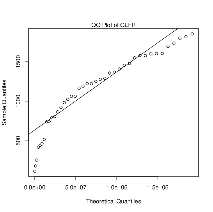
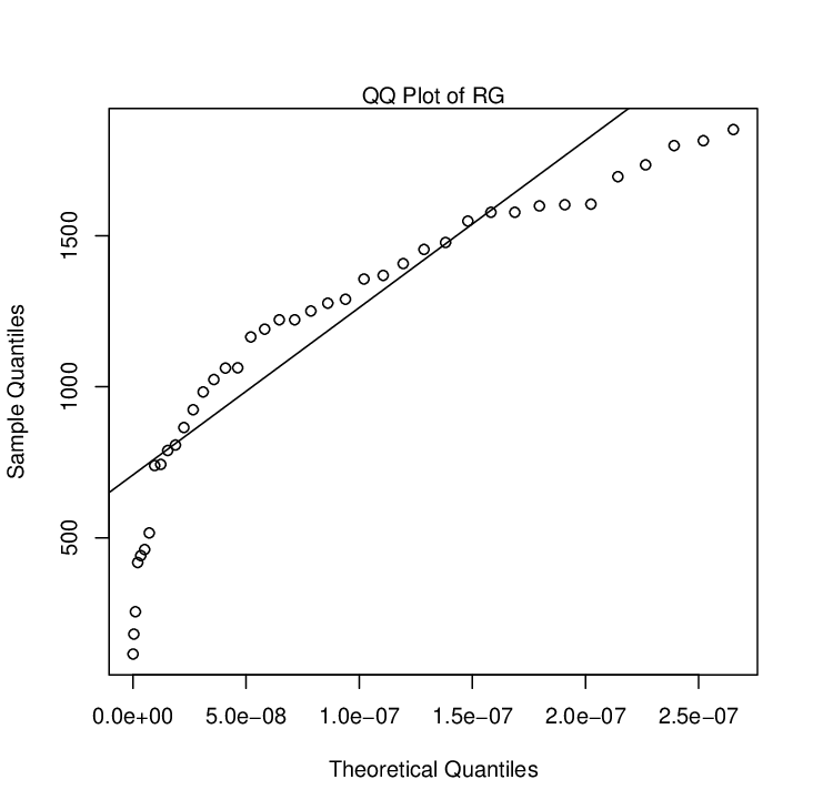
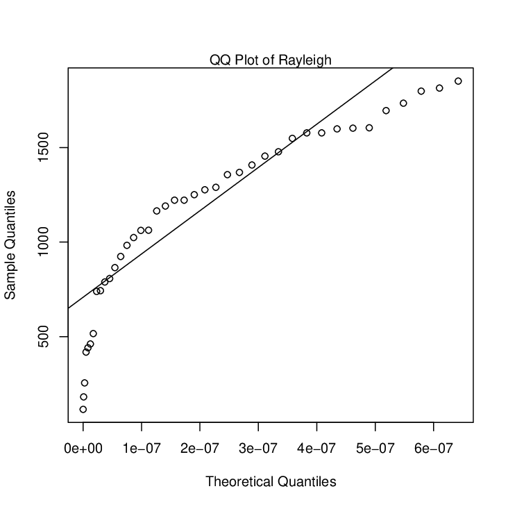
Plots of the estimated pdf, cdf and survival function with the qq-plot of fitted distributions are given in Fig. 7 and Fig. 8, respectively. These plots suggest that the LFRG distribution is superior to the other distributions in terms of model fitting.
For parametric comparisons, we have used the likelihood ratio (LR) test statistics, , to test the null hypotheses against the alternative one mentioned above. Table 6 gives the null hypothesis , the value of log-likelihood function under , , the value of the likelihood ratio test statistics, , the degree of freedom of , df, and the corresponding p-value. From the p-values it is clear that we reject at level of significance , at level of significance , at level of significance , at level of significance and at any level of significance. This concludes that the LFRG distribution is the best among all distributions used here to fit the current data set.

| Model | MLEs | S.E. | C.I. | -2log L | AIC | AICC | BIC | K-S | P-value | AD | CM |
| =7.73E-4 | 5.3E-4 | (-0.0003,0.0018) | |||||||||
| LFRG | =2.05E-6 | 4.3E-7 | (1.3E-6,2.9E-6) | 604.0 | 610.0 | 610.6 | 615.0 | 0.0831 | 0.9450 | 0.4381 | 0.1304 |
| =-8.448 | 2.1E-8 | (-8.448,-8.448) | |||||||||
| =2.1E-4 | 3.6E-4 | (-0.0005,0.0009) | |||||||||
| GLFR | =1.4E-6 | 6.2E-7 | (1.7E-7,2.6E-6) | 610.7 | 616.7 | 617.3 | 621.7 | 0.1481 | 0.3440 | 1.1053 | 0.2687 |
| =1.5528 | 0.6108 | (0.3183,2.7873) | |||||||||
| LFR | =1E-8 | 8.1E-9 | (-5.8E-9,2.6E-8) | 612.0 | 616.0 | 612.3 | 619.4 | 0.1659 | 0.2210 | 1.5019 | 0.3719 |
| =1.3E-6 | 1.1E-7 | (1.1E-6,1.5E-6) | |||||||||
| EG | =0.00338 | 0.0005 | (0.0024,0.0044) | 607.5 | 611.5 | 611.8 | 614.8 | 0.0882 | 0.9150 | 0.6151 | 0.1484 |
| =-48.64 | 34.028 | (-117.41,20.130) | |||||||||
| RG | =2.48E-6 | 2.5E-7 | (2E-6,3E-6) | 607.1 | 611.1 | 611.5 | 614.1 | 0.0959 | 0.8550 | 0.6543 | 0.1446 |
| =-3.57 | 0.09136 | (-3.749,-3.391) | |||||||||
| Rayleigh | =1.3E-6 | 1.5E-8 | (1.3E-6,1.35E-6) | 612.0 | 614.0 | 614.1 | 615.7 | 0.1659 | 0.2210 | 1.5018 | 0.3719 |
| Exp | =8.8E-4 | 1.4E-4 | (0.0006,0.0012) | 642.9 | 644.9 | 645.0 | 646.6 | 0.3031 | 0.0013 | 1.2102 | 5.7083 |
| Model | df | P-value | |||
| LFR | 306 | 8 | 1 | 0.0018 | |
| EG | 303.75 | 3 | 1 | 0.1987 | |
| RG | 303.55 | 3.1 | 1 | 0.1844 | |
| Rayleigh | , | 306 | 8 | 2 | 0.0190 |
| Exp | , | 321.45 | 38.9 | 2 | 8.3E-19 |
| LFRG | = | 302 | – | – | – |




8 Conclusion
We introduce a new class of lifetime distributions called the linear failure rate-power series (LFRPS) class of distributions, which generalizes the linear failure rate (LFR) distribution and is obtained by compounding the LFR distribution and power series (PS) class of distributions. This new class of distributions contains some new distributions such as linear failure rate geometric (LFRG) distribution, linear failure rate Poisson (LFRP) distribution, linear failure rate logarithmic (LFRL) distribution, linear failure rate binomial (LFRB) distribution and Raylight-power series (RPS) class of distributions. Some former works such as exponential-power series (EPS) class of distributions (Chahkandi and Ganjali, 2009), exponential geometric (EG) distribution (Adamidis and Loukas, 1998), exponential Poisson (EP) distribution (Kuş, 2007), and exponential logarithmic (EL) distribution (Tahmasbi and Rezaei, 2008) are special cases of the new proposed model.
The ability of the new proposed model is in covering five possible hazard rate function i.e., increasing, decreasing, upside-down bathtub (unimodal), bathtub and increasing-decreasing-increasing shaped. Several properties of the LFRPS distributions such as moments, maximum likelihood estimation procedure via an EM-algorithm and inference for a large sample, are discussed in this paper. In order to show the flexibility and potentiality of the new class of distributions, the fitted results of the new class of distributions and some its submodels are compared using a real data set.
Appendix A
Let and . Then
Appendix B
B.1
Let
where , , , and .
i. If , then, is strictly decreasing in and
Therefore,
and
Therefore, when , and when . Hence, the proof is completed.
ii. If , then, is strictly increasing in and
Therefore,
and
Therefore, when , and when . Then, for a given , and , the root of lies in the following interval:
B.2
Let
i. For LFRP, it is clear that
Therefore, the equation has at least one root for , if or .
ii. For LFRG, it is clear that
Therefore, the equation has at least one root for , if or .
iii. For LFRL, it is clear that
Therefore, the equation has at least one root for , if or .
iv.It is clear that
Therefore, the equation has at least one root for , if and or and .
Appendix C
C.1
We can easily show that is decreasing function with respect to . Also
Therefore, the root of is unique. It can easily show that
Therefore, when , and when . Hence, the proof is completed.
C.2
We can easily show that is decreasing function with respect to . Also
Therefore, the root of is unique. It can easily show that
Therefore, when , and when . Hence, the proof is completed.
C.3
i. For LFRG distribution, . Therefore, the root of
is unique and is equal to , and
Let
Therefore, is increasing function and
If , then . Therefore, , and .
ii. For LFRP distribution, . Therefore,
Since
where and and also,
therefore, has a minimum value at , and . Thus, the root of is unique.
For LFRL distribution, . Therefore,
Since
where and and also,
therefore, has a minimum value at , and . Thus, the root of is unique.
For LFRB distribution, . Therefore,
Since
where and and also,
therefore, has a minimum value at , and . Thus, the root of is unique.
References
- Abouammoh et al. (1994) Abouammoh, A. M., Abdulghani, S. A., Qamber, I. S., 1994. On partial orderings and testing of new better than renewal used classes. Reliability Engineering & System Safety 43 (1), 37–41.
- Adamidis et al. (2005) Adamidis, K., Dimitrakopoulou, T., Loukas, S., 2005. On an extension of the exponential-geometric distribution. Statistics and Probability Letters 73 (3), 259–269.
- Adamidis and Loukas (1998) Adamidis, K., Loukas, S., 1998. A lifetime distribution with decreasing failure rate. Statistics and Probability Letters 39 (1), 35–42.
- Barreto-Souza et al. (2011) Barreto-Souza, W., de Morais, A. L., Cordeiro, G. M., 2011. The weibull-geometric distribution. Journal of Statistical Computation and Simulation 81 (5), 645–657.
- Bourguignon et al. (2012) Bourguignon, M., Silva, R. B., Cordeiro, G. M., 2012. A new class of fatigue life distributions. arXiv preprint arXiv:1212.0707.
- Chahkandi and Ganjali (2009) Chahkandi, M., Ganjali, M., 2009. On some lifetime distributions with decreasing failure rate. Computational Statistics and Data Analysis 53 (12), 4433–4440.
- Dempster et al. (1977) Dempster, A. P., Laird, N. M., Rubin, D. B., 1977. Maximum likelihood from incomplete data via the EM algorithm. Journal of the Royal Statistical Society. Series B (Methodological) 39 (1), 1–38.
- Flores et al. (2011) Flores, J., Borgesb, P., Cancho, V. G., Louzada, F., 2011. The complementary exponential power series distribution. Brazilian Journal of Probability and Statistics (accepted).
- Ghitany and Kotz (2007) Ghitany, M. E., Kotz, S., 2007. Reliability properties of extended linear failure-rate distributions. Probability in the Engineering and Informational Sciences 21 (3), 441–450.
- Johnson et al. (2005) Johnson, N. L., Kemp, A. W., Kotz, S., 2005. Univariate discrete distributions, 3rd Edition. Wiley-Interscience.
- Kuş (2007) Kuş, C., 2007. A new lifetime distribution. Computational Statistics and Data Analysis 51 (9), 4497–4509.
- Louis (1982) Louis, T. A., 1982. Finding the observed information matrix when using the EM algorithm. Journal of the Royal Statistical Society. Series B (Methodological) 44 (2), 226–233.
- Lu and Shi (2011) Lu, W., Shi, D., 2011. A new compounding life distribution: the Weibull–poisson distribution. Journal of Applied Statistics 39 (1), 21–38.
- Mahmoudi and Jafari (2012) Mahmoudi, E., Jafari, A. A., 2012. Generalized exponential-power series distributions. Computational Statistics and Data Analysis 56 (12), 4047–4066.
- Mahmoudi and Sepahdar (2013) Mahmoudi, E. and Sepahdar, A., 2013. Exponentiated Weibull-Poisson distribution: model, properties and applications. Mathematics and Computers in Simulation 92, 76–97.
- Marshall and Olkin (1997) Marshall, A. W., Olkin, I., 1997. A new method for adding a parameter to a family of distributions with application to the exponential and Weibull families. Biometrika 84 (3), 641–652.
- Morais and Barreto-Souza (2011) Morais, A. L., Barreto-Souza, W., 2011. A compound class of Weibull and power series distributions. Computational Statistics and Data Analysis 55 (3), 1410–1425.
- Nadarajah and Mitov (2005) Nadarajah, S., Mitov, K., 2005. Correction: A new response time distribution. Biometrics 61 (1), 311.
- Noack (1950) Noack, A., 1950. A class of random variables with discrete distributions. The Annals of Mathematical Statistics 21 (1), 127–132.
- Sen and Bhattacharyya (1995) Sen, A., Bhattacharyya, G. K., 1995. Inference procedures for the linear failure rate model. Journal of Statistical Planning and Inference 46 (1), 59–76.
- Silva et al. (2013) Silva, R. B., Bourguignon, M., Dias, C. R. B., Cordeiro, G. M., 2013. The compound class of extended Weibull power series distributions. Computational Statistics and Data Analysis 58, 352–367.
- Tahmasbi and Rezaei (2008) Tahmasbi, R., Rezaei, S., 2008. A two-parameter lifetime distribution with decreasing failure rate. Computational Statistics and Data Analysis 52 (8), 3889–3901.