Towards Automatic Stress Analysis using Scaled Boundary Finite Element Method with Quadtree Mesh of High-order Elements
Abstract
This paper presents a technique for stress and fracture analysis by using the scaled boundary finite element method (SBFEM) with quadtree mesh of high-order elements. The cells of the quadtree mesh are modelled as scaled boundary polygons that can have any number of edges, be of any high orders and represent the stress singularity around a crack tip accurately without asymptotic enrichment or other special techniques. Owing to these features, a simple and automatic meshing algorithm is devised. No special treatment is required for the hanging nodes and no displacement incompatibility occurs. Curved boundaries and cracks are modelled without excessive local refinement. Five numerical examples are presented to demonstrate the simplicity and applicability of the proposed technique.
Keywords:
scaled boundary finite-element method; quadtree mesh; high order elements; polygon elements1 Introduction
Finite Element Analysis (FEA) is the most widely used analysing tool in Computer Aided Engineering (CAE). One key factor to achieve an accurate FEA is the layout of the finite element mesh, including both mesh density and element shape [1]. Regions containing complex boundaries, rapid transitions between geometric features or singularities require finer discretisation [2, 3]. This leads to the development of adaptive meshing techniques that assure the solution accuracy without sacrificing the computational efficiency [4, 5]. The construction of a high quality mesh, in general, takes the most of the analysis time [6]. The recent rapid development of the isogeometric analysis [6, 7, 8], which suppressed the meshing process, has emphasised the significance of mesh automation in engineering design and analysis.
Quadtree in FEA is a kind of hierarchical tree-based techniques for adaptive meshing of a 2D geometry [3]. It discretises the geometry into a number of square cells of different size. The process is illustrated in Fig. 1 using a circular domain. The geometry is first covered with a single square cell, also known as the root cell of the quadtree (Fig. 1a). As shown in Fig. 1b, the root cell is subdivided into 4 equal-sized square cells and each of the cells is recursively subdivided to refine the mesh until certain termination criteria are reached. In this example, a cell is subdivided to better represent the boundary of the circle and the subdivision stops when the predefined maximum number of division is reached. The final mesh is obtained after deleting all the cells outside the domain (Fig. 1c). The cell information is stored in a tree-type data structure, in which the root cell is at the highest level. It is common practice to limit the maximum difference of the division levels between two adjacent cells to one [1, 9]. This is referred to the rule and the resulting mesh is called a balanced [9] or restricted quadtree mesh [4]. A balanced quadtree mesh not only ensures there is no large size difference between adjacent cells, but also reduces the types of quadtree cells in a mesh to the 6 shown in Fig. 2. Owing to its simplicity and large degree of flexibility, the quadtree mesh is also recognised in large-scale flood/tsunami simulations [10, 11] and image processing [12].


It is, however, not straightforward to integrate a quadtree mesh in a FEA. The two major issues are illustrated by Fig. 3, which shows the quadtree mesh of the top-right quadrant of the circular domain in Fig. 1.
- 1.
Hanging nodes Middle nodes, shown as solid dots in Fig. 3, exist at the common edges between the adjacent cells with different division levels. When conventional quadrilateral finite elements are used, a middle node is connected to the two smaller elements (lower level) but not to the larger element (higher level). This leads to incompatible displacement along the edges and the middle nodes are called the hanging nodes [3].
- 2.
Fitting of curved boundary Quadtree cells are composed of horizontal and vertical lines only. As shown in Fig. 3, the quadtree cells intersected with the curved boundary have to be further divided into smaller ones to improve the fitting of the boundary. Generally, the mesh has to be refined in the area surrounding the boundary. Despite this, the boundary may still not be smooth (Fig. 1c) and may result in unrealistically high stresses. Additional procedure is required to conform the mesh to the boundary.
There exist a number of different approaches to ensure displacement compatibility when hanging nodes are present [13, 14, 15, 16]. Three typical approaches among all are briefly discussed here. The first one is to subdivide the higher level quadtree cells next to a hanging node into smaller triangular elements [1, 17, 18] as shown in Fig 3. Additional nodes may be added to improve the mesh quality and/or reduce the number of element types. These techniques lead to a final mesh that only contains conforming triangular elements. A similar approach was adpoted by Ebeida et al. [13], in which the quadtree mesh was subdivided into a conforming mesh dominated by quadrilateral elements.
The second approach introduces special conforming shape functions [19] to ensure the displacement compatibility. An early work by Gupta [19] reported the development of a transition element that had additional node along its side. A conforming set of shape functions was derived based on the shape functions of the bilinear quadrilateral elements. Owing to its simplicity and applicability, Gupta’s work was further extended by Mcdill et al. [20] and Lo et al. [5] to hexahedral elements. Fries et al. [21] investigated two approaches to handle the hanging nodes within the framework of the extended finite element method (XFEM). They were different in whether the enriched degrees-of-freedom (DOFs) were assigned to the hanging node. A similar work was reported by Legrain et al. [14], in which the selected DOFs are enriched and properly constrained to ensure the continuity of the field.

The third approach is to model the quadtree cells as n-sided polygon elements by treating hanging nodes as vertices of the polygon. This approach generally requires a set of polygonal basis function. Special techniques are usually required to integrate the resulting equations over arbitrary polygon domain [22]. This development was initiated by Wachspress [23] who showed the use of rational basis functions for elements with arbitrary number of sides. Tabarraei and Sukumar [4, 24] in their work adapted their polygon element [25] to quadtree mesh. The set of polygonal basis functions was derived using Laplace interpolant. By using an affine map on the reference polygon, the conforming shape functions of a quadtree cell with the same number of vertices (including the hanging nodes) were obtained. They also reported a fast technique for computing the global stiffness matrix, making use of the quadtree structure by defining parent elements [24]. In this way, the elemental stiffness matrix has to be computed only 15 times (4-node cell not included) for a balanced quadtree mesh (when rule is enforced). Further development of their work with XFEM was also reported in [15].
As mentioned in a recent paper [26], the development of high-order polygon elements received relatively less attention. Mibradt and Pick [27] devised high order basis functions for polygons based on the natural element coordinates. Those basis functions, however, are not complete polynomials. Rand et al. [28] developed a quadratic serendipity element for arbitrary convex polygons based on generalised barycentric coordinates. The potential of using their approach for higher order serendipity elements on convex polygons was also reported. Based on the same approach, Sukumar [26] recently developed the quadratic serendipity shape functions that were applicable for convex and nonconvex polygons and were complete quadratic polynomials. The shape functions were obtained through solving an optimisation problem, which was derived from the maximum-entropy principle.
Besides dealing with the hanging nodes in a quadtree mesh, fitting complex boundaries is another challenging part in the mesh generation. Yerry and Shephard [1] proposed trimming the quadtree cells, intersected with the boundary, into polygons before a further subdivision process into triangles or quadrilaterals. Alternatively those cells were first subdivided and some of the vertices were repositioned based on their projections onto the boundary [3, 18]. In Ebeida et al. [13] and Liang et al. [29], after the subdivision, a buffer zone was introduced between the boundary and the internal quadtree cells. A compatible mesh was then constructed to fill up this zone. All these techniques require an additional optimisation step to ensure the final mesh quality. Within the framework of XFEM, quadtree cells intersected with the boundary were not modified in pre-processing stage [21]. However, when constructing the stiffness matrix, the domain boundary is still required to identify the portion of the cell within the domain for numerical integration. In the integration process, that portion of the cell within the domain is either subdivided into geometric sub-cells [30] or treated as a polygon [31].
The scaled boundary finite element method (SBFEM) provides an attractive alternate technique to construct polygon elements (scaled boundary polygon) [32, 33] (Fig. 4). It is a semi-analytical procedure developed by Song and Wolf to solve boundary value problems [34]. The only requirement for a scaled boundary polygon is that its entire boundary is visible from the scaling centre [34]. Only the edges of the polygon are discretised into line elements. The number of line elements on an edge can be as many as required. Any type of displacement-based line elements, including high-order spectral elements [35], can be used. The domain of the scaled boundary polygon is constructed by scaling from its scaling centre to its boundary, and the solution within the polygon is expressed semi-analytically [32, 33]. A salient feature of the scaled boundary polygons is that stress singularities occurring at crack and notch tips, formed by one or several materials, can be accurately modelled without resorting to asymptotic enrichment and local mesh refinement. Its high accuracy and flexibility in mesh generation lead to simple remeshing procedures when modelling crack propagation [36, 37, 38, 33].


This paper presents a technique for the stress and fracture analysis by integrating the scaled boundary finite element method (SBFEM) with quadtree mesh of high-order elements. This integrated technique possesses the following features:
- 1.
Hanging nodes are treated without cell subdivision. Each quadtree cell is modelled as a scaled boundary polygon as shown in Fig. 5. The edges of a quadtree cell can be divided into more than one line element to ensure displacement compatibility with the adjacent smaller cells. Hanging-nodes are thus treated the same as other nodes. Owing to the SBFE formulations [32], no additional procedure is required to compute the shape functions for the quadtree cells. High-order elements can also be used within each quadtree cell directly.
- 2.
The entire quadtree meshing process is simple and automatic. The boundary of the problem domain is defined using signed distance functions [39]. Only seed points [3] are required to be predefined to control the mesh density. Owing to the ability of the SBFEM in constructing polygon elements of, practically, arbitrary shape and order, the quadtree cells trimmed by curved boundaries are simply treated as a non-square scaled boundary polygon. High-order elements can be used to fit curved boundaries closely. The resulting mesh conforms to the boundary without excessive mesh refinement (see Fig. 5).
- 3.
No local mesh refinement or asymptotic enrichment is required for a quadtree cell containing a crack tip to accurately model the stress singularity.
The present paper is organised as follows. The summary of the SBFEM and its application to quadtree cells are first presented in the next section. It is followed by the developed algorithm of quadtree mesh generation in Section 3. Five examples are given in Section 4 with detailed discussion on accuracy and convergence. Finally, conclusions of the present work are stated in Section 5.
2 Scaled boundary finite element method on quadtree cells
This section summarises the scaled boundary finite element method for 2D stress and fracture analysis. Only the key equations that are related to its use with a quadtree mesh are listed. A detailed derivation of the method based on a virtual work approach is given in Deeks and Wolf [40].
2.1 Element formulation
The SBFEM can be formulated on quadtree cells by treating each cell as a polygon with arbitrary number of sides (Fig. 5). In each cell, a local coordinate system is defined at a point called the scaling centre from which the entire boundary is visible. is the radial coordinate with at the scaling centre and at the cell boundary. The edges of each cell are discretised using one-dimensional finite elements with a local coordinate having an interval of . It is noted that the hanging nodes appearing in the quadtree structure do not require any special treatment in the SBFEM formulation. They are simply used as end nodes of the 1D elements.
The coordinate transformation between the Cartesian and the local coordinate systems are given by the scaled boundary transformation equations [34]:
| (1) |
where is the Cartesian coordinates of a point in the cell, is the shape function matrix and is the vector of nodal coordinates of a cell with nodes.
The displacement field in each cell is interpolated as
| (2) |
where are radial displacement functions and are obtained by solving the scaled boundary finite element equation in displacement [34]:
| (3) |
with coefficient matrices
| (4) | ||||
| (5) | ||||
| (6) |
where is the material constitutive matrix, and are the SBFEM strain-displacement matrices and is the Jacobian on the boundary required for coordinate transformation.
where
| (8) |
so that Eq. (3) is transformed into a first order ordinary differential equation with twice the number of unknowns:
| (9) |
with the Hamiltonian matrix [41]
An eigenvalue decomposition of the results in
where and are the eigenvalue matrices with real parts satisfying and , respectively. and are the corresponding eigenvectors of whereas and are the eigenvectors corresponding to . For bounded domains such as those considered in this paper, only the eigenvalues satisfying lead to finite displacements at the scaling centre. Using Eq. (2.1) and Eq. (9), the solutions for and are
| (18) | ||||
| (19) |
The integration constants in Eq. (18) and Eq. (19) are obtained from the nodal displacements at the cell boundary as
| (20) |
The stiffness matrix of each quadtree cell is formulated as [41]
| (21) |
Using the Hooke’s law and the strain-displacement relationship, the stress at a point in a cell is [41]
| (23) |
where is the stress mode
| (24) |
2.2 Evaluation of stress intensity factors
Fig. 6 shows how a crack is modelled with a quadtree cell. The crack tip is chosen as the scaling centre. The crack surfaces are not discretised. The line elements discretising the cell boundary do not form a closed loop.

When a crack is modelled by the SBFEM, two eigenvalues, , satisfying appear in . From Eq. 23, it can be discovered that these eigenvalues lead to a stress singularity as . Using the two modes corresponding to these two eigenvalues, the singular stresses are expressed as
| (25) |
where
and are the integration constants corresponding to . The singular singular stress modes is written as
| (28) |
where are the modal displacements in corresponding to .
The stress intensity factors can be computed directly from their definitions. For a crack that is aligned with the Cartesian coordinate system as shown in Fig. 6, the stress intensity factors are defined as
3 Quadtree mesh generation
This section presents the developed algorithm for quadtree mesh generation. Fig. 7 shows the flow chart of the overall process. The entire generation process is automatic with minimal number of inputs required from the user, which include
- 1.
Maximum allowed number of seed points in a cell ,
- 2.
Seed points on each boundary and region of interest ,
- 3.
Maximum difference between the division levels of adjacent cells , which is equal to 1 for a balanced quadtree mesh.

This section is organised based on Fig 7. It first presents defining geometry using signed distance function, and assigning seed points on the boundary and the regions of interest. Detailed explanations of the meshing steps, which include generating the initial quadtree grid, trimming the boundary quadtree cells into polygons and merging cells surrounding a crack tip, are then followed. To facilitate the description of the meshing steps, Fig. 8 shows a square plate with a circular hole and two local refinement features to be used as an example throughout this section. An efficient computation of the global stiffness matrix, by taking advantage on the quadtree mesh, is described at the end of this section.

3.1 Define geometry using signed distance function
The geometry is defined by using the signed distance function [42]. It provides all the essential information of a geometry and can be operated with simple Boolean operations to build up more complex geometries [39]. The signed distance function of a point associated with a domain , which is a subset of , is given as
| (37) |
where represents the boundary of the domain and is the Euclidean norm in with . The sign function is equal when lies inside the domain and is equal 1 otherwise. This definition of the signed distance function is visualised in Fig. 9. A number of distance functions in MATLAB for simple geometries are given in Talischi et al. [39], including their Boolean operations.

For each boundary and region of interest, a set of pre-defined seed points [3] is introduced to control the quadtree mesh density. There require four sets of predefined seed points for the example in Fig. 8. Two sets are for the square and the circular hole representing the actual domain boundary. The number of seed points directly controls the local density of the quadtree cells and the quality of fitting the boundary. This is further discussed in Section 3.3. The other two sets are for the large circle and inclined line controlling local mesh density only.
3.2 Initialise quadtree grid
The meshing process starts with covering the problem domain with a single square cell (the root cell). The dimension of the root cell is based on the larger one between the maximum vertical and maximum horizontal dimension of the geometry. The developed algorithm will check the number of seed points in the cell. If the number is larger than the predefined maximum allowed number, the cell will be divided into 4 equal-sized cells. This generation process is applied recursively until all the cells have seed points no more than the predefined value. For each recursive loop, the maximum difference between the division levels of adjacent cells is enforced. For cells that have division level difference with the adjacent cells larger than , the higher level cell is subdivided into 4 equal-sized cells. Fig. 10 shows the initial quadtree grid of the example in Fig. 8.

3.3 Trim boundary cells into polygons
The initial quadtree grid shown in Fig. 10 does not conform to the boundary. Those cells that have edges intersected with the boundary need to be identified and trimmed. By using the signed distance function, the locations of the vertices (inside the domain, on the domain boundary or outside the domain as shown in Fig. 10) are identified based on the sign and value of the function. For edges containing two vertices with opposite signs, they are identified as the edges intersected with the boundary. For each of those edges, the intersection point with the boundary is computed.
Some quadtree cells could have vertices very close to the boundary in comparison with the lengths of their edges. After trimming, poorly shaped polygon cells with some edges much shorter than the others could be generated and may adversely affect the mesh quality. To avoid this situation, the vertices that are within a threshold distance away from the boundary are identified and then moved to their closest points on the boundary. In the present work, of the length of the cell edge (based on the smallest cell attaching to the vertex) is used as the threshold value. The edges connecting to these vertices will no longer be cut by the boundary. The trade-off of this process is the presence of additional non-square cells that lead to additional computation of the stiffness matrix. This is discussed in Section 3.5.

At the end of the trimming process, the edges of a cell cut by the boundary are updated with the intersection points and the enclosed segment of boundary is added to the cell. This will result in polygon cells. After trimming the quadtree in Fig. 10, the polygon cells around the hole of the example problem is shown in Fig. 11. It is clear from Fig. 11 that the circular boundary is not represented accurately if a single linear element is used on the edge of the cell.
In order to represent the curved boundary more accurately, two alternates are available in the developed algorithm. The first is to reduce the element size (-refinement). This is achieved by increasing the number of seed points on the curved boundary. Fig. 12 shows the initial quadtree layout of the example problem after increasing the seed points around the hole by 4 times. It can be seen by comparing Fig. 10 with Fig. 12 that the refinement is limited to a small region around the hole. The refined quadtree (Fig 11) demonstrates the improvement of capturing the circular boundary.

The second option to improve the modelling of curved boundaries is to utilise high-order elements (-refinement). Fig. 11 shows the example problem with each line segment on the circular boundary modelled with a 4th order element. With this approach, curved boundaries can be captured more accurately using fewer elements.
Both options to improve the modelling of the boundaries can be applied simultaneously without conflicts. The numerical accuracy of both approaches is discussed through numerical examples given in Section 4.
3.4 Merge cells surrounding a crack tip
Owing to the capability of the SBFEM for fracture analysis [43], the domain containing a crack tip is modelled with a single cell. In the stress solution, the variation along the radial direction, including the stress singularity, is given analytically and the variation along the circumference of the cell is represented numerically by the line elements on boundary. To obtain accurate results, sufficient nodes have to present on the boundary of the cell to cover the angular variation of the solution . In the developed algorithm, the size of a cell containing a crack tip is controlled, as shown in Fig. 13 with an inclined crack, by a predefined set of seed points on a circle.

For problems with cracks, only one additional step is required after the initial mesh is generated. The cells surrounding the crack tip are refined to the same division level and then merged into a single cell as shown in Fig. 13. This step avoids having a crack tip too close to the edges of the cell, which could affect the mesh quality and the solution accuracy [38]. After the cells are merged, the intersection point between the edge of the resulting cell and the crack is computed to define the two crack mouth points. The other cells on the crack path are split by the crack into two cells. The splitting process is similar to the trimming of cells by the boundary, but two vertices are created at every intersection point between the cell edge and the crack to split the original cells.
3.5 An efficient construction of the global stiffness matrix
The global stiffness matrix is simply the assembly of the stiffness matrices of each master quadtree and polygon cell. When the rule is enforced to the mesh, only 6 main types of master quadtree cells are present as given in Fig. 2. By rotating the geometry of the master cells orthogonally, the maximum number of types of these master quadtree cells are 24. For isotropic homogeneous materials, rotation does not have effect on 4-node or 8-node cells and only two 2 rotations are required for the first type of 6-node cell (the top one in Fig. 2). The maximum number of master quadtree cells that require stiffness matrix calculation reduces to 16 (only 15 in Tabarraei and Sukumar [24] as 4-node cell is excluded).
After the mesh generation, the algorithm will check which master cells out of the 16 appear in the mesh. Their stiffness matrices are then computed and stored. During the stiffness assembling process, the stiffness matrix of each regular quadtree cell is directly extracted from those computed stiffness matrices. For the polygon cells and those irregular quadtree cells (with their vertices moved to fit the boundaries), individual stiffness matrix calculation is required. This approach clearly improves the computational efficiency of constructing the global stiffness matrix, especially for large scale problems that contain a significant number of cells. With the use of high-order elements in the quadtree mesh, this assembling approach becomes even more economical.
4 Numerical examples
This section presents five numerical examples to highlight the capability and the performance of the proposed technique. In the first example, an infinite plate with a circular hole is modelled and the results are compared with the analytical solution. The proposed technique is then used to analyse a square plate with multiple holes to highlight the automatic meshing capability in handling transition between geometric features. In the third example, a square plate with a central hole and multiple cracks is studied to demonstrate the performance of the proposed technique in handling complicated geometries with singularities. Thereafter, a square plate with two cracks cross each other is analysed. It is aimed to emphasise the automation and simplicity of the mesh generation in the proposed technique. In the first four examples, the same material properties, with Young’s modulus and Poisson’s ratio , are used. The final example is a cracked nuclear reactor under internal pressure. It is aimed to show the simplicity of the present technique in modelling practical non-regular structures.
The computation time reported in this section is based on a desktop PC with Intel(R) Core(TM) i7 3.40GHz CPU and 16GB of memory. The proposed technique is implemented in MATLAB and the computation time is extracted in interactive mode of MATLAB.
4.1 Infinite plate with a circular hole under uniaxial tension
4.1.1 Modelling using exact boundary condition
An infinite plate containing a circular hole with radius at its centre is considered in this example. The plate is subject to a uniaxial tensile load as shown in Fig. 14. The analytical solution of the stresses in polar coordinates is given by [44]:
| (38) | ||||
The displacement solutions are:
| (39) |
where is the shear modulus and is the Kolosov constant for plane stress condition.
The problem is solved by analysing a finite dimension of the plate with a dimension of (see Fig. 14). Analytical traction (Eq. 38) is applied at the four edges of this finite plate.


Fig. 15(a) shows the quadtree mesh of the plate for . Each edge on a quadtree cell is discretised with 1st order line elements. The rule is enforced. Based on the proposed technique, the curved boundary is handled as shown in Fig. 15(b) with polygon cells. Convergence study is conducted based on the refinement. Three different element orders are investigated.
Fig. 16 shows the present results of the relative error in the displacement norm , with the analytical solution given in Eq. (39) and the solution computed by the proposed technique. The results show that all three types of elements have monotonic convergence. For higher order elements, more accurate results with similar number of DOF are obtained and the convergence rate is also faster.

There are 37 out of 100 cells calculated for the stiffness matrices. Among those 37 cells, 9 are regular quadtree cells and 28 are polygon cells surrounding the hole. For the remaining cells, their stiffness matrices are simply extracted from those 9 regular quadtree cells.
To further demonstrate the accuracy of the proposed technique, along (see Fig. 14) is plotted in Fig. 17 using the mesh given in Fig. 15(a) with 4th order elements. It can be seen that the results of the proposed technique agree well with the analytical solution, which has at (). For points away from , approaches 1.

4.1.2 Approximation of infinite plate by varying ratio
The same infinite plate can be approximated by increasing the ratio. The application of quadtree mesh facilitates such a study. Only the left and right sides of the plate are subjected to uniaxial in-plane tension stress . The element order used in this study is . The same mesh given in Fig. 15(a) is used for . The adaptive capability of quadtree mesh leads to the same mesh pattern for all ratios. Fig. 18 shows the cells around the hole for and it is exactly the same as the one shown in Fig. 15(b).
For , although there are 316 cells in total, only 37 cells are calculated for the stiffness matrices, which is the same as the previous study. The results of at with varying ratio are given in Table 1. It is seen that the analytical solution () is quickly approached when increasing the ratio.

| ratio | No. of Nodes | at |
|---|---|---|
| 10 | 860 | 3.3591 |
| 40 | 1428 | 3.0204 |
| 160 | 1996 | 3.0049 |
| 640 | 2564 | 2.9991 |
4.2 Square plate with multiple holes
A unit square plate with 9 randomly distributed holes of different sizes, shown in Fig. 19, is analysed. This example highlights the automation and flexibility of the proposed technique in handling the mesh transition between features with various dimensions. The ability of capturing curved boundaries accurately using high-order elements is also demonstrated. The displacements at the bottom edge of the plate are fully constrained and a uniform tension is applied at the top edge of the plate. A set of consistent units are chosen.

To validate the results, the same problem is solved using the commercial FEA software ANSYS V14.5. The plate is discretised using 8-node quadrilateral elements (PLANE183). In order to demonstrate the automation and performance of the proposed technique, similar user inputs are given to ANSYS to generate a mesh for comparison.
In ANSYS, the square plate is divided into 4 equal-sized quadrants such that a centre key point is created for result comparison. The 9 holes are introduced to the plate by subtracting their areas from the square plate. The mesh constructed in ANSYS is unstructured (paving). A single variable is used to control the mesh density and is used for mesh refinement. For each hole, the number of element around them is equal to . And for all the straight lines, the size of the elements is set to be , which gives each outer edge approximately elements. Note that the mesh used in ANSYS is far from optimal and structured mesh should be used for better performance. However, the main objective using paving mesh and only controlling the boundary element divisions is to show how the proposed technique and ANSYS perform when minimal number of controlling variables are used for the meshing. For the proposed technique, seed points with , where is the maximum allowed number of seed points in a cell, are set on the circular holes to generate a mesh with similar number of boundary division as the one in ANSYS.
Fig. 20 shows the ANSYS mesh (1358 elements) and the quadtree mesh (1169 cells). Both meshes can effectively handle the mesh transition between the holes. As commented earlier, while the mesh in ANSYS can be further improved by designing a structured layout, it would also require additional time and investigation effort. The amount of additional effort depends on the complexity of the geometry and user experience. And for the proposed technique, the resulting mesh is always in a structured manner (see Fig. 20(b)) without additional effort. The time of generating the quadtree mesh is around 3s using the computer with details outlined in the beginning of this section.


For the stiffness calculation, there are 364 out of 1169 cells calculated. Among those 364 cells, 12 are master quadtree cells and 352 are polygon cells surrounding the holes. The stiffness matrices for all the other cells are simply extracted from the calculated master quadtree cells. The total time from constructing the stiffness to obtaining the displacement solutions is less than 3.2s when using 5th order elements.
Table 2 shows the convergence of the displacement components at the centre point with increasing element order using mesh in Fig. 20(b). In order to highlight the convergence performance, Fig. 21 shows the relative error of the present results of the displacement vector sum at point . The error is calculated based on the converged ANSYS results, which converged to the first 6 significant digits. Also shown in the same figure are the relative errors of the ANSYS results and another set of results of the proposed technique. They are both generated through a series of refinement with the use of 2nd order elements. It is observed that the present results with refinement converge with the fastest rate. And for the refinement, the present results are basically converging at the same rate as those of ANSYS with slightly better accuracy. The present results demonstrate that for the same accuracy, much less number of DOFs is required when using high-order elements, and curved boundaries are also accurately modelled with minimal number of cells.
| Elem. Order | No. of Nodes | at | at |
|---|---|---|---|
| 2 | 4379 | 4.98298 | 6.67236 |
| 3 | 7157 | 4.98350 | 6.67359 |
| 4 | 9935 | 4.98241 | 6.67374 |
| 5 | 12713 | 4.98197 | 6.67379 |

In order to further demonstrate the overall consistency of the present results, Fig. 22 shows the contour plots of , from both ANSYS and the proposed technique. Good agreement is observed from the contour plots.


4.3 Square plate with multiple cracks emanating from a hole
A square plate of length with a centre hole of radius of given in Fig. 23 is considered. cracks with crack length emanate from the hole. This example aims to show the simplicity and effectiveness of the proposed technique to solve problems with singularities.

In this example, to approach the assumption of an infinite plate, is considered. A parametric study is performed considering cracks surrounding the hole with various ratio. The element order used in this study is , which is capable to model the circular boundary accurately as shown in the first example. The present results are compared with the reference solution of the stress intensity factor given in Tada et al. [45].
Fig. 24 shows the mesh around the central hole, with 4 and 8 cracks around the edge and . Based on the proposed technique, no refinement is required around the crack tips. This facilitates the study with multiple cracks and results in less computational effort when comparing to the conventional FEM.


Fig. 25 shows the stress intensity factor () computed from the proposed technique for different value of . Excellent agreement with the reference solution [45] is observed. This demonstrates the accuracy of the proposed technique in dealing with stress singularities as well as the feasibility in handling geometry with complicated features.

4.4 Square plate with two cracks cross each other
A square plate of length with two cracks cross each other is considered. The dimensions of the plate and the cracks as well as the boundary conditions are shown in Fig. 26. This example highlights the automatic mesh generation of the proposed technique and the capacity to handle problems with complicated crack configuration.

Fig. 27 shows the quadtree mesh of the proposed technique. The mesh only requires defining seed points on the domain boundary, along the cracks and around the crack tips to control the quadtree mesh density. The mesh generation is fully automatic without the requirement of dividing area regions. The resulting mesh contains a total of 216 cells. During the construction of the stiffness matrix, only 48 cells are computed, which contains 9 master quatree cells and 39 polygon cells.
For the same problem, it would require a few more steps to generate a mesh in FEA. These include defining crack tip regions that directly affect the solution accuracy, and designing proper refinement strategy that directly affects the convergence performance. For example in ANSYS, a command “KSCON” needs to be issued to each crack tip in order to generate two circular layers of elements (1 layer singular elements) around the tip. The radius of the two circular layers of elements is solely based on user experience and trial-and-error. Shape warning on the elements would occur if the settings of that command are not consistent with the global mesh. Moreover, automatic refinement is not applicable when “KSCON” is activated. It would, therefore, require multiple steps to conduct convergence study with refinement, such as reducing the radius of the circular layers of element around the crack tips and increasing elements in circumferential direction around the crack tips.

Table 3 shows the crack opening displacements ( and in Fig. 26) with increasing element order. Similar to previous examples, the present results converge rapidly with minimal number of nodes increased. The results between using the 2nd order elements and using the 5th order elements are different with less than .
| Elem. Order | No. of Nodes | ||
|---|---|---|---|
| 2 | 818 | 5.1300 | 6.9710 |
| 3 | 1333 | 5.1274 | 6.9727 |
| 4 | 1848 | 5.1279 | 6.9726 |
| 5 | 2363 | 5.1280 | 6.9725 |
4.5 Cracked nuclear reactor under internal pressure
In this final example, a nuclear reactor under internal pressure [8] is analysed. Due to symmetry, only a quadrant of the reactor is modelled. The geometry, material properties, loading and dimension are shown in Fig. 28. Also shown in the figure are the two cracks introduced on the outer boundary. This example shows the flexibility of the proposed technique and the developed meshing algorithm to model more practical structures.
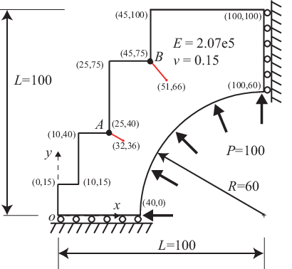
Fig. 29 shows the quadtree mesh used in this example, which contains a total of 160 cells. Using the proposed technique only requires seed points to be defined at the boundaries to control the quadtree mesh density. No additional requirement for the cells containing the crack tips is necessary. The time spent on generating the quadtree mesh is less than 0.8s using the same computer with details outlined in the beginning of this section.
The calculation of stiffness matrix involves computing 44 out of the 160 cells, in which 12 are master quadtree cells and 32 are polygon cells. The total time from constructing the stiffness matrix to obtaining the displacement solution is less than 0.7s when using 5th order elements.

A convergence study is conducted by increasing the order of the element without changing the quadtree layout in Fig. 29. Table 4 shows the two crack opening displacements at points and (Fig. 28). The present results converge quickly with the element order increased. The difference between using the 2nd order elements and using the 5th order elements is less than 0.1%. This further highlights the advantage of using high-order elements that can model curved boundary more accurately with minimal number of cells.
| Elem. Order | No. of Nodes | ||
|---|---|---|---|
| 2 | 635 | 7.14372 | 2.60404 |
| 3 | 1031 | 7.15066 | 2.60336 |
| 4 | 1427 | 7.15077 | 2.60334 |
| 5 | 1823 | 7.15077 | 2.60332 |
5 Conclusion
This paper has presented a numerical technique to automate stress and fracture analysis using the SBFEM and quadtree mesh of high-order elements. Owing to the nature of the SBFEM, the proposed technique has no specific requirement, such as deriving conforming shape functions or sub-triangulation, to handle quadtree cells with hanging nodes. High-order elements are used within each quadtree cell directly.
The quadtree mesh generation is fully automatic and involves minimal number of user inputs and operation steps. Boundaries are modelled with scaled boundary polygons and this allows the proposed technique to conform the boundary without excessive mesh refinement. The meshing algorithm is also applicable for problems with singularities. The use of quadtree mesh leads to an efficient approach to compute the global stiffness matrix. This facilitates the analysis that requires a significant number of cells using high-order elements. Five numerical examples are presented to highlight the functionality and performance of the proposed technique. The present results show excellent agreement with analytical solutions and those computed by the FEM.
Reference
References
- [1]
M. Yerry, M. Shephard, A modified quadtree approach to finite element mesh
generation, IEEE Computer Graphics and Applications 3 (1) (1983) 39–46.
- [2]
G. Cheng, H. Li, New method for graded mesh generation of quadrilateral finite
elements, Computers & Structures 59 (5) (1996) 823–829.
- [3]
D. M. Greaves, A. G. L. Borthwick, Hierarchical tree-based finite element mesh
generation, International Journal for Numerical Methods in Engineering 45
(1999) 447–471.
- [4]
A. Tabarraei, N. Sukumar, Adaptive computations on conforming quadtree
meshes, Finite Elements in Analysis and Design 41 (7-8) (2005) 686–702.
- [5]
S. Lo, D. Wu, K. Sze, Adaptive meshing and analysis using transitional
quadrilateral and hexahedral elements, Finite Elements in Analysis and
Design 46 (1-2) (2010) 2–16.
- [6]
T. Hughes, J. Cottrell, Y. Bazilevs, Isogeometric analysis: CAD, finite
elements, NURBS, exact geometry and mesh refinement, Computer Methods in
Applied Mechanics and Engineering 194 (39-41) (2005) 4135–4195.
- [7]
N. Nguyen-Thanh, H. Nguyen-Xuan, S. Bordas, T. Rabczuk, Isogeometric analysis
using polynomial splines over hierarchical T-meshes for two-dimensional
elastic solids, Computer Methods in Applied Mechanics and Engineering
200 (21-22) (2011) 1892–1908.
- [8]
R. Simpson, S. Bordas, H. Lian, J. Trevelyan, An isogeometric boundary element
method for elastostatic analysis: 2D implementation aspects, Computers &
Structures 118 (2013) 2–12.
- [9]
P. R. GVS, H. J. Montas, H. Samet, A. Shirmohammadi, Quadtree-Based Triangular
Mesh Generation for Finite Element Analysis of Heterogeneous Spatial Data,
in: The 2001 ASAE Annual International Meeting (Paper ID:01-3072),
Sacramento, CA, 2001.
- [10]
Q. Liang, G. Du, J. Hall, A. Borthwick, Flood inundation modeling with an
adaptive quadtree grid shallow water equation solver, Journal of Hydraulic
Engineering 134 (2008) 1603–1610.
- [11]
S. Popinet, Quadtree-adaptive tsunami modelling, Ocean Dynamics 61 (9) (2011)
1261–1285.
- [12]
Y. Morvan, D. Farin, Depth-Image Compression Based on An RD Optimized Quadtree
Decomposition For The Transmission of Multiview Images, IEEE International
Conference on Image Processing, ICIP 2007, 5 (2007) V105–V108.
- [13]
M. S. Ebeida, R. L. Davis, R. W. Freund, A new fast hybrid adaptive grid
generation technique for arbitrary two-dimensional domains, International
Journal for Numerical Methods in Engineering 84 (2010) 305–329.
- [14]
G. Legrain, R. Allais, P. Cartraud, On the use of the extended finite element
method with quadtree/octree meshes, International Journal for Numerical
Methods in Engineering 86 (2011) 717–743.
- [15]
A. Tabarraei, N. Sukumar, Extended finite element method on polygonal and
quadtree meshes, Computer Methods in Applied Mechanics and Engineering 197
(2008) 425–438.
- [16]
M. Ainsworth, L. Demkowicz, C.-W. Kim, Analysis of the equilibrated residual
method for a posteriori error estimation on meshes with hanging nodes,
Computer Methods in Applied Mechanics and Engineering 196 (37-40) (2007)
3493–3507.
- [17]
M. Bern, D. Eppstein, J. Gilbert, Provably good mesh generation, Journal of
Computer and System Sciences 48 (3) (1994) 384–409.
- [18]
B. Alyavuz, O. Kocyigit, T. Gultop, Numerical solution of seepage problem
using quad-tree based triangular finite elements, International Journal of
Engineering and Applied Sciences 1 (1) (2009) 43–56.
- [19]
A. K. Gupta, A finite element for transition from a fine to a coarse grid,
International Journal for Numerical Methods in Engineering 12 (1978) 35–45.
- [20]
J. M. Mcdill, J. A. Goldak, A. S. Oddy, M. J. Bibby, Isoparametric
quadrilaterals and hexahedrons for mesh-grading algorithms, Communications
in Applied Numerical Methods 3 (1987) 155–163.
- [21]
T. Fries, A. Byfut, A. Alizada, K. Cheng, A. Schroder, Hanging nodes and
xfem, International Journal for Numerical Methods in Engineering 86 (2011)
404–430.
- [22]
S. Natarajan, S. Bordas, D. Roy Mahapatra, Numerical integration over
arbitrary polygonal domains based on Schwarz-Christoffel conformal mapping,
International Journal for Numerical Methods in Engineering 80 (2009)
103–134.
- [23]
E. L. Wachspress, A rational finite element basis, Academic Press, New York,
1975.
- [24]
A. Tabarraei, N. Sukumar, Adaptive computations using material forces and
residual-based error estimators on quadtree meshes, Computer Methods in
Applied Mechanics and Engineering 196 (25-28) (2007) 2657–2680.
- [25]
N. Sukumar, a. Tabarraei, Conforming polygonal finite elements, International
Journal for Numerical Methods in Engineering 61 (12) (2004) 2045–2066.
- [26]
N. Sukumar, Quadratic maximum-entropy serendipity shape functions for
arbitrary planar polygons, Computer Methods in Applied Mechanics and
Engineering 263 (2013) 27–41.
- [27]
P. Milbradt, T. Pick, Polytope finite elements, International Journal for
Numerical Methods in Engineering 73 (2008) 1811–1835.
- [28]
A. Rand, A. Gillette, C. Bajaj, Quadratic Serendipity Finite Elements on
Polygons Using Generalized Barycentric Coordinates, Mathematics of
Computation in press.
- [29]
X. Liang, M. S. Ebeida, Y. Zhang, Guaranteed-quality all-quadrilateral mesh
generation with feature preservation, Computer Methods in Applied Mechanics
and Engineering 199 (29-32) (2010) 2072–2083.
- [30]
K. Dréau, N. Chevaugeon, N. Moës, Studied X-FEM enrichment to handle
material interfaces with higher order finite element, Computer Methods in
Applied Mechanics and Engineering 199 (29-32) (2010) 1922–1936.
- [31]
S. Natarajan, D. Roy Mahapatra, S. P. A. Bordas, Integrating strong and weak
discontinuities without integration subcells and example applications in an
XFEM/GFEM framework, International Journal for Numerical Methods in
Engineering 83 (2010) 269–294.
- [32]
E. T. Ooi, C. Song, F. Tin-Loi, Z. J. Yang, Polygon scaled boundary finite
elements for crack propagation modelling, International Journal for
Numerical Methods in Engineering 91 (2012) 319–342.
- [33]
E. T. Ooi, M. Shi, C. Song, F. Tin-Loi, Z. J. Yang, Dynamic crack propagation
simulation with scaled boundary polygon elements and automatic remeshing
technique, Engineering Fracture Mechanics 106 (2012) (2013) 1–21.
- [34]
C. Song, J. P. Wolf, The scaled boundary finite-element method–alias
consistent infinitesimal finite-element cell method–for elastodynamics,
Computer Methods in applied mechanics and engineering 147 (3-4) (1997)
329–355.
- [35]
T. H. Vu, A. J. Deeks, Use of higher-order shape functions in the scaled
boundary finite element method, International Journal for Numerical Methods
in Engineering 65 (10) (2006) 1714–1733.
- [36]
Z. J. Yang, Fully automatic modelling of mixed-mode crack propagation using
scaled boundary finite element method, Engineering Fracture Mechanics 73
(2006) 1711–1731.
- [37]
E. T. Ooi, Z. J. Yang, Modelling multiple cohesive crack propagation using a
finite element–scaled boundary finite element coupled method, Engineering
Analysis with Boundary Elements 33 (7) (2009) 915–929.
- [38]
E. T. Ooi, Z. J. Yang, A hybrid finite element-scaled boundary finite element
method for crack propagation modelling, Computer Methods in Applied
Mechanics and Engineering 199 (17-20) (2010) 1178–1192.
- [39]
C. Talischi, G. H. Paulino, A. Pereira, I. F. M. Menezes, PolyMesher: a
general-purpose mesh generator for polygonal elements written in Matlab,
Structural and Multidisciplinary Optimization 45 (3) (2012) 309–328.
- [40]
A. J. Deeks, J. P. Wolf, A virtual work derivation of the scaled boundary
finite-element method for elastostatics, Computational Mechanics 28 (6)
(2002) 489–504.
- [41]
J. P. Wolf, The scaled boundary finite element method, Wiley Chichester (W.
Sx.), 2003.
- [42]
P. Persson, G. Strang, A simple mesh generator in MATLAB, SIAM Review 46 (2)
(2004) 329–345.
- [43]
C. Song, J. P. Wolf, Semi-analytical representation of stress singularities as
occurring in cracks in anisotropic multi-materials with the scaled boundary
finite-element method, Computers & structures 80 (2) (2002) 183–197.
- [44]
N. Sukumar, D. L. Chopp, N. Moes, T. Belytschko, Modeling holes and inclusions
by level sets in the extended finite-element method, Computer Methods in
Applied Mechanics and Engineering 190 (2001) 6183–6200.
- [45]
H. Tada, P. C. Paris, G. R. Irwin, The stress analysis of cracks handbook,
ASME press, New York, 2000.
References
- [1] M. Yerry, M. Shephard, A modified quadtree approach to finite element mesh generation, IEEE Computer Graphics and Applications 3 (1) (1983) 39–46.
- [2] G. Cheng, H. Li, New method for graded mesh generation of quadrilateral finite elements, Computers & Structures 59 (5) (1996) 823–829.
- [3] D. M. Greaves, A. G. L. Borthwick, Hierarchical tree-based finite element mesh generation, International Journal for Numerical Methods in Engineering 45 (1999) 447–471.
- [4] A. Tabarraei, N. Sukumar, Adaptive computations on conforming quadtree meshes, Finite Elements in Analysis and Design 41 (7-8) (2005) 686–702.
- [5] S. Lo, D. Wu, K. Sze, Adaptive meshing and analysis using transitional quadrilateral and hexahedral elements, Finite Elements in Analysis and Design 46 (1-2) (2010) 2–16.
- [6] T. Hughes, J. Cottrell, Y. Bazilevs, Isogeometric analysis: CAD, finite elements, NURBS, exact geometry and mesh refinement, Computer Methods in Applied Mechanics and Engineering 194 (39-41) (2005) 4135–4195.
- [7] N. Nguyen-Thanh, H. Nguyen-Xuan, S. Bordas, T. Rabczuk, Isogeometric analysis using polynomial splines over hierarchical T-meshes for two-dimensional elastic solids, Computer Methods in Applied Mechanics and Engineering 200 (21-22) (2011) 1892–1908.
- [8] R. Simpson, S. Bordas, H. Lian, J. Trevelyan, An isogeometric boundary element method for elastostatic analysis: 2D implementation aspects, Computers & Structures 118 (2013) 2–12.
- [9] P. R. GVS, H. J. Montas, H. Samet, A. Shirmohammadi, Quadtree-Based Triangular Mesh Generation for Finite Element Analysis of Heterogeneous Spatial Data, in: The 2001 ASAE Annual International Meeting (Paper ID:01-3072), Sacramento, CA, 2001.
- [10] Q. Liang, G. Du, J. Hall, A. Borthwick, Flood inundation modeling with an adaptive quadtree grid shallow water equation solver, Journal of Hydraulic Engineering 134 (2008) 1603–1610.
- [11] S. Popinet, Quadtree-adaptive tsunami modelling, Ocean Dynamics 61 (9) (2011) 1261–1285.
- [12] Y. Morvan, D. Farin, Depth-Image Compression Based on An RD Optimized Quadtree Decomposition For The Transmission of Multiview Images, IEEE International Conference on Image Processing, ICIP 2007, 5 (2007) V105–V108.
- [13] M. S. Ebeida, R. L. Davis, R. W. Freund, A new fast hybrid adaptive grid generation technique for arbitrary two-dimensional domains, International Journal for Numerical Methods in Engineering 84 (2010) 305–329.
- [14] G. Legrain, R. Allais, P. Cartraud, On the use of the extended finite element method with quadtree/octree meshes, International Journal for Numerical Methods in Engineering 86 (2011) 717–743.
- [15] A. Tabarraei, N. Sukumar, Extended finite element method on polygonal and quadtree meshes, Computer Methods in Applied Mechanics and Engineering 197 (2008) 425–438.
- [16] M. Ainsworth, L. Demkowicz, C.-W. Kim, Analysis of the equilibrated residual method for a posteriori error estimation on meshes with hanging nodes, Computer Methods in Applied Mechanics and Engineering 196 (37-40) (2007) 3493–3507.
- [17] M. Bern, D. Eppstein, J. Gilbert, Provably good mesh generation, Journal of Computer and System Sciences 48 (3) (1994) 384–409.
- [18] B. Alyavuz, O. Kocyigit, T. Gultop, Numerical solution of seepage problem using quad-tree based triangular finite elements, International Journal of Engineering and Applied Sciences 1 (1) (2009) 43–56.
- [19] A. K. Gupta, A finite element for transition from a fine to a coarse grid, International Journal for Numerical Methods in Engineering 12 (1978) 35–45.
- [20] J. M. Mcdill, J. A. Goldak, A. S. Oddy, M. J. Bibby, Isoparametric quadrilaterals and hexahedrons for mesh-grading algorithms, Communications in Applied Numerical Methods 3 (1987) 155–163.
- [21] T. Fries, A. Byfut, A. Alizada, K. Cheng, A. Schroder, Hanging nodes and xfem, International Journal for Numerical Methods in Engineering 86 (2011) 404–430.
- [22] S. Natarajan, S. Bordas, D. Roy Mahapatra, Numerical integration over arbitrary polygonal domains based on Schwarz-Christoffel conformal mapping, International Journal for Numerical Methods in Engineering 80 (2009) 103–134.
- [23] E. L. Wachspress, A rational finite element basis, Academic Press, New York, 1975.
- [24] A. Tabarraei, N. Sukumar, Adaptive computations using material forces and residual-based error estimators on quadtree meshes, Computer Methods in Applied Mechanics and Engineering 196 (25-28) (2007) 2657–2680.
- [25] N. Sukumar, a. Tabarraei, Conforming polygonal finite elements, International Journal for Numerical Methods in Engineering 61 (12) (2004) 2045–2066.
- [26] N. Sukumar, Quadratic maximum-entropy serendipity shape functions for arbitrary planar polygons, Computer Methods in Applied Mechanics and Engineering 263 (2013) 27–41.
- [27] P. Milbradt, T. Pick, Polytope finite elements, International Journal for Numerical Methods in Engineering 73 (2008) 1811–1835.
- [28] A. Rand, A. Gillette, C. Bajaj, Quadratic Serendipity Finite Elements on Polygons Using Generalized Barycentric Coordinates, Mathematics of Computation in press.
- [29] X. Liang, M. S. Ebeida, Y. Zhang, Guaranteed-quality all-quadrilateral mesh generation with feature preservation, Computer Methods in Applied Mechanics and Engineering 199 (29-32) (2010) 2072–2083.
- [30] K. Dréau, N. Chevaugeon, N. Moës, Studied X-FEM enrichment to handle material interfaces with higher order finite element, Computer Methods in Applied Mechanics and Engineering 199 (29-32) (2010) 1922–1936.
- [31] S. Natarajan, D. Roy Mahapatra, S. P. A. Bordas, Integrating strong and weak discontinuities without integration subcells and example applications in an XFEM/GFEM framework, International Journal for Numerical Methods in Engineering 83 (2010) 269–294.
- [32] E. T. Ooi, C. Song, F. Tin-Loi, Z. J. Yang, Polygon scaled boundary finite elements for crack propagation modelling, International Journal for Numerical Methods in Engineering 91 (2012) 319–342.
- [33] E. T. Ooi, M. Shi, C. Song, F. Tin-Loi, Z. J. Yang, Dynamic crack propagation simulation with scaled boundary polygon elements and automatic remeshing technique, Engineering Fracture Mechanics 106 (2012) (2013) 1–21.
- [34] C. Song, J. P. Wolf, The scaled boundary finite-element method–alias consistent infinitesimal finite-element cell method–for elastodynamics, Computer Methods in applied mechanics and engineering 147 (3-4) (1997) 329–355.
- [35] T. H. Vu, A. J. Deeks, Use of higher-order shape functions in the scaled boundary finite element method, International Journal for Numerical Methods in Engineering 65 (10) (2006) 1714–1733.
- [36] Z. J. Yang, Fully automatic modelling of mixed-mode crack propagation using scaled boundary finite element method, Engineering Fracture Mechanics 73 (2006) 1711–1731.
- [37] E. T. Ooi, Z. J. Yang, Modelling multiple cohesive crack propagation using a finite element–scaled boundary finite element coupled method, Engineering Analysis with Boundary Elements 33 (7) (2009) 915–929.
- [38] E. T. Ooi, Z. J. Yang, A hybrid finite element-scaled boundary finite element method for crack propagation modelling, Computer Methods in Applied Mechanics and Engineering 199 (17-20) (2010) 1178–1192.
- [39] C. Talischi, G. H. Paulino, A. Pereira, I. F. M. Menezes, PolyMesher: a general-purpose mesh generator for polygonal elements written in Matlab, Structural and Multidisciplinary Optimization 45 (3) (2012) 309–328.
- [40] A. J. Deeks, J. P. Wolf, A virtual work derivation of the scaled boundary finite-element method for elastostatics, Computational Mechanics 28 (6) (2002) 489–504.
- [41] J. P. Wolf, The scaled boundary finite element method, Wiley Chichester (W. Sx.), 2003.
- [42] P. Persson, G. Strang, A simple mesh generator in MATLAB, SIAM Review 46 (2) (2004) 329–345.
- [43] C. Song, J. P. Wolf, Semi-analytical representation of stress singularities as occurring in cracks in anisotropic multi-materials with the scaled boundary finite-element method, Computers & structures 80 (2) (2002) 183–197.
- [44] N. Sukumar, D. L. Chopp, N. Moes, T. Belytschko, Modeling holes and inclusions by level sets in the extended finite-element method, Computer Methods in Applied Mechanics and Engineering 190 (2001) 6183–6200.
- [45] H. Tada, P. C. Paris, G. R. Irwin, The stress analysis of cracks handbook, ASME press, New York, 2000.