Optimal Geo-Indistinguishable Mechanisms for
Location Privacy

A common way of achieving location privacy is to apply a location obfuscation mechanism, that is a probabilistic function $K:\mathcal{X}\to\mathcal{P}(\mathcal{X})$ where $\mathcal{X}$ is the set of possible locations, and $\mathcal{P}(\mathcal{X})$ denotes the set of probability distributions over $\mathcal{X}$. $K$ takes a location $x$ as input, and produces a reported location $z$ which is communicated to the service provider. In this paper we generally consider $\mathcal{X}$ to be finite, in which case $K$ can be represented by a stochastic matrix, where $k_{xz}$ is the probability to report $z$ from location $x$.

A prior distribution $\pi\in\mathcal{P}(\mathcal{X})$ on the set of locations can be viewed either as modelling the behaviour of the user (the user profile), or as capturing the adversary’s side information about the user. Given a prior $\pi$ and a metric $d$ on $\mathcal{X}$, the expected distance between the real and the reported location is:

From the user’s point of view, we want to quantify the service quality loss (QL) produced by the mechanism $K$. Given a quality metric $d_{Q}$ on locations, such that $d_{Q}(x,z)$ measures how much the quality decreases by reporting $z$ when the real location is $x$ (the Euclidean metric ${d_{2}}$ being a typical choice), we can naturally define the quality loss as the expected distance between the real and the reported location, that is $\textsc{QL}(K,\pi,d_{Q})=\textsc{ExpDist}(K,\pi,d_{Q})$. The QL can also be viewed as the (inverse of the) utility of the mechanism.

Similarly, we want to quantify the privacy provided by $K$. A natural approach, introduced in [10] is to consider a Bayesian adversary with some prior information $\pi$, trying to remap $z$ back to a guessed location $\hat{x}$. A remapping strategy can be modelled by a stochastic matrix $H$, where $h_{z\hat{x}}$ is the probability to map $z$ to $\hat{x}$. Then the privacy of the mechanism can be defined as the expected error of an adversary under the best possible remapping:

Note that the composition $KH$ of $K$ and $H$ is itself a mechanism. Similarly to $d_{Q}$, the metric $d_{A}(x,\hat{x})$ captures the adversary’s loss when he guesses $\hat{x}$ while the real location is $x$. Note that $d_{Q}$ and $d_{A}$ can be different, but the canonical choice is to use the Euclidean distance for both.

A natural question, then, is to construct a mechanism that achieves optimal privacy, given a QL constraint.

In other words, a $q$-OptPriv mechanism provides the best privacy (expressed in terms of AdvError) among all mechanisms with QL at most $q$. This problem was studied in [8], providing a method to construct such a mechanism for any $q,\pi,d_{A},d_{Q}$, by solving a properly constructed linear program.

Differential privacy was originally introduced in the context of statistical databases, requiring that a query should produce similar results when applied to adjacent databases, i.e. those differing by a single row. The notion of adjacency is related to the Hamming metric ${d_{h}}(x,x^{\prime})$ defined as the number of rows in which $x,x^{\prime}$ differ. Differential privacy requires that the greater the hamming distance between $x,x^{\prime}$ is, the more distinguishable they are allowed to be.

This concept can be naturally extended to any set of secrets $\mathcal{X}$, equipped with a metric ${d_{\scriptscriptstyle\mathcal{X}}}$ [14, 12]. The distance ${d_{\scriptscriptstyle\mathcal{X}}}(x,x^{\prime})$ expresses the distinguishability level between $x$ and $x^{\prime}$: if the distance is small then the secrets should remain indistinguishable, while secrets far away from each other are allowed to be distinguished by the adversary. The metric should be chosen depending on the application at hand and the semantics of the privacy notion that we try to achieve.

Following the notation of [12], a mechanism is a probabilistic function $K:\mathcal{X}\to\mathcal{P}(\mathcal{Z})$, where $\mathcal{Z}$ is a set of reported values (assumed finite for the purposes of this paper). The similarity between probability distributions can be measured by the multiplicative distance ${d_{\mathcal{P}}}$ defined as $d_{\cal P}(\mu_{1},\mu_{2})=\sup_{z\in\mathcal{Z}}|\ln\frac{\mu_{1}(z)}{\mu_{2}(z)}|$ with $|\ln\frac{\mu_{1}(z)}{\mu_{2}(z)}|=0$ if both $\mu_{1}(z),\mu_{2}(z)$ are zero and $\infty$ if only one of them is zero. In other words, ${d_{\mathcal{P}}}(\mu_{1},\mu_{2})$ is small iff $\mu_{1},\mu_{2}$ assign similar probabilities to each value $z$.

The generalized variant of differential privacy under the metric ${d_{\scriptscriptstyle\mathcal{X}}}$, called ${d_{\scriptscriptstyle\mathcal{X}}}$-privacy, is defined as follows:

or equivalently $K(x)(z)\leq e^{{d_{\scriptscriptstyle\mathcal{X}}}(x,x^{\prime})}K(x^{\prime})(z)$ for all $x,x^{\prime}\in\mathcal{X},z\in\mathcal{Z}$. A privacy parameter $\epsilon$ can also be introduced by scaling the metric ${d_{\scriptscriptstyle\mathcal{X}}}$ (note that $\epsilon{d_{\scriptscriptstyle\mathcal{X}}}$ is itself a metric).

Differential privacy can then be expressed as $\epsilon{d_{h}}$-privacy. Moreover, different metrics give rise to various privacy notions of interest; several examples are given in [12].

In the context of location based systems the secrets $\mathcal{X}$ are locations, and we can obtain a useful notion of location privacy by naturally using the Euclidean distance ${d_{2}}$, scaled by a security parameter $\epsilon$. The resulting notion of $\epsilon{d_{2}}$-privacy, called $\epsilon$-geo-indistinguishability in [9], requires that a location obfuscation mechanism should produce similar results when applied to locations that are geographically close. This prevents the service provider from inferring the user’s location with accuracy, while allowing him to get approximate information required to provide the service. Following the spirit of differential privacy, this definition is independent from the prior information of the adversary.

A characterization of geo-indistinguishability from [9] provides further intuition about this notion. The characterization compares the adversary’s conclusions (a posterior distribution) to his initial knowledge (a prior distribution). Since some information is supposed to be revealed (i.e. the provider will learn that the user is somewhere around Paris), we cannot expect the two distributions to coincide. However, geo-indistinguishability implies that an informed adversary who already knows that the user is located within a small area $N$, cannot improve his initial knowledge and locate the user with higher accuracy. More details, together with a second characterization can be found in [9].

Note that geo-indistinguishability does not guarantee a small leakage under any prior; in fact no obfuscation mechanism can ensure this while offering some utility. Consider, for instance, an adversary who knows that the user is located at some airport, but not which one. Unless the noise is huge, reporting an obfuscated location will allow the exact location to be inferred, but this is unavoidable.¹¹ 1 This example is the counterpart of the well-known Terry Gross example from [11].

Considering the mechanism, [9] shows that geo-indistinguishability can be achieved by adding noise to the user’s location drawn from a 2-dimensional Laplace distribution. This can be easily done in polar coordinates by selecting and angle uniformly and a radius from a Gamma distribution. If a restricted set of reported locations is allowed, then the location produced by the mechanism can be mapped back to the closest among the allowed ones.

Although the Laplace mechanism provides an easy and practical way of achieving geo-indistinguishability, independently from any user profile, its utility is not always optimal. In the next section we show that by tailoring a mechanism to a prior corresponding to a specific user profile, we can achieve better utility for that prior, while still satisfying geo-indistinguishability, i.e. a privacy guarantee independent from the prior. The evaluation results in Section 4 show that the optimal mechanism can provide substantial improvements compared to the Laplace mechanism.

The constructed mechanism is assumed to have as both input and output a predetermined finite set of locations $\mathcal{X}$. For instance, $\mathcal{X}$ can be constructed by dividing the map in a finite number of regions (of arbitrary size and shape), and selecting in $\mathcal{X}$ a representative location for each region. We also assume a prior $\pi$ over $\mathcal{X}$, representing the probability of the user being at each location at any given time.

Given a privacy metric ${d_{\scriptscriptstyle\mathcal{X}}}$ (typically the Euclidean distance) and a privacy parameter $\epsilon$, the goal is to construct a $\epsilon{d_{\scriptscriptstyle\mathcal{X}}}$-private mechanism $K$ such that the service quality loss with respect to a quality metric $d_{Q}$ is minimum. This property is formally defined below:

Note that $\epsilon{d_{\scriptscriptstyle\mathcal{X}}}$-OptQL optimizes QL given a privacy constraint, while $q$-OptPriv (Definition 1) optimizes privacy, given an QL constraint.

In order for $K$ to be $\epsilon{d_{\scriptscriptstyle\mathcal{X}}}$-private it should satisfy the following constraints:

Hence, we can construct an optimal mechanism by solving a linear optimization problem, minimizing $\textsc{QL}(K,\pi,d_{Q})$ while satisfying $\epsilon{d_{\scriptscriptstyle\mathcal{X}}}$-privacy:

It is easy to see that the mechanism $K$ generated by the previous optimization problem is $\epsilon{d_{\scriptscriptstyle\mathcal{X}}}$-$\textsc{OptQL}(\pi,d_{Q})$.

In the optimization problem of the previous section, the $\epsilon{d_{\scriptscriptstyle\mathcal{X}}}$-privacy definition introduces $|\mathcal{X}|^{3}$ constraints in the linear program. However, in order to be able to manage a large number of locations, we would like to reduce this amount to a number in the order of $O(|\mathcal{X}|^{2})$. One possible way to achieve this is to use the dual form of the linear program (shown in the appendix). The dual program has as many constraints as the variables of the primal program (in this case $|\mathcal{X}|^{2}$) and one variable for each constraint in the primal program (in this case $O(|\mathcal{X}|^{3})$). Since the primal linear program finds the optimal solution in a finite number of steps, it is guaranteed by the strong duality theorem that dual program will also do so. However, as shown in Section 4.3, in practice the dual program does not offer a substantial improvement with respect to the primal one (a possible explanation being that, although fewer in number, the constrains in the dual program are more complex, in the sense that each one of them involves a larger number of variables).

An alternative approach is to exploit the structure of the metric ${d_{\scriptscriptstyle\mathcal{X}}}$. So far we are not making any assumption about ${d_{\scriptscriptstyle\mathcal{X}}}$, and therefore we need to specify $|\mathcal{X}|$ constraints for each pair of locations $x$ and $x^{\prime}$. However, it is worth noting that if the distance ${d_{\scriptscriptstyle\mathcal{X}}}$ is induced by a weighted graph (i.e. the distance between each pair of locations is the weight of a minimum path in a graph), then we only need to consider $|\mathcal{X}|$ constraints for each pair of locations that are adjacent in the graph. An example of this is the usual definition of differential privacy: since the adjacency relation between databases induces the Hamming distance $d_{h}$, we only need to require the differential privacy constraint for each pair of databases that are adjacent in the Hamming graph (i.e. that differ in one individual).

It might be the case, though, that the metric ${d_{\scriptscriptstyle\mathcal{X}}}$ is not induced by any graph (other than the complete graph), and consequently the amount of constraints remains the same. In fact, this is generally the case for the Euclidean metric. Therefore, we consider the case in which ${d_{\scriptscriptstyle\mathcal{X}}}$ can be approximated by some graph-induced metric.

If $G$ is an undirected weighted graph, we denote with $d_{G}$ the distance function induced by $G$, i.e. $d_{G}(x,x^{\prime})$ denotes the weight of a minimum path between the nodes $x$ and $x^{\prime}$ in $G$. Then, if the set of nodes of $G$ is $\mathcal{X}$ and the weight of its edges is given by the metric ${d_{\scriptscriptstyle\mathcal{X}}}$, we can approximate ${d_{\scriptscriptstyle\mathcal{X}}}$ with $d_{G}$. In this case, we say that $G$ is a spanning graph, or a spanner [15, 16], of $\mathcal{X}$.

Note that if $G$ is a spanner of $\mathcal{X}$, then

A main concept in the theory of spanners is that of dilation, also known as stretch factor:

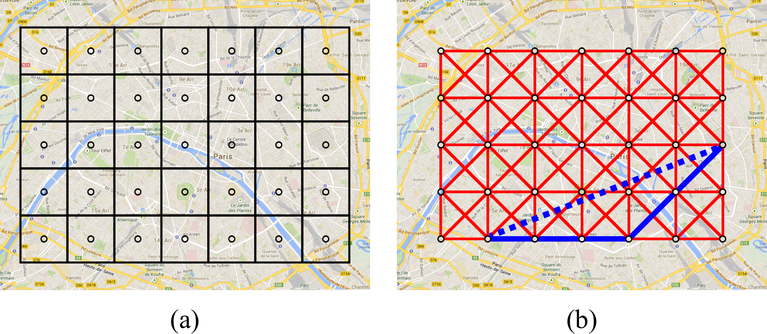
Informally, a $\delta$-spanner of $\mathcal{X}$ can be considered an approximation of the metric ${d_{\scriptscriptstyle\mathcal{X}}}$ in which distances between nodes are “stretched” by a factor of at most $\delta$. Spanners are generally used to approximate distances in a geographic network without considering the individual distances between each pair of nodes. An example of a spanner for a grid in the map can be seen in Figure 1.

If $G$ is a $\delta$-spanner of $\mathcal{X}$, then it holds that

which leads to the following proposition:

We can then propose a new optimization problem to obtain a $\epsilon{d_{\scriptscriptstyle\mathcal{X}}}$-private mechanism. If $G=(\mathcal{X},E)$ is a $\delta$-spanner of $\mathcal{X}$, we require not the constraints corresponding to $\epsilon{d_{\scriptscriptstyle\mathcal{X}}}$-privacy, but those corresponding to $\frac{\epsilon}{\delta}d_{G}$-privacy instead, that is, $|\mathcal{X}|$ constraints for each edge of $G$:

Since the resulting mechanism is $\frac{\epsilon}{\delta}d_{G}$-private, by Proposition 1 it must also be $\epsilon{d_{\scriptscriptstyle\mathcal{X}}}$-private. However, the number of constraints in induced by $\frac{\epsilon}{\delta}d_{G}$-privacy is now $|E||\mathcal{X}|$. Moreover, as discussed in the next section, for any $\delta>1$ there is an algorithm that generates a $\delta$-spanner with $O(\frac{|\mathcal{X}|}{\delta-1})$ edges, which means that, fixing $\delta$, the total number of constraints of the linear program is $O(|\mathcal{X}|^{2})$.

It is worth noting that although $\epsilon{d_{\scriptscriptstyle\mathcal{X}}}$-privacy is guaranteed, optimality is lost: the obtained mechanism is $\frac{\epsilon}{\delta}d_{G}$-$\textsc{OptQL}(\pi,d_{Q})$ but not necessarily $\epsilon{d_{\scriptscriptstyle\mathcal{X}}}$-$\textsc{OptQL}(\pi,d_{Q})$, since the set of $\frac{\epsilon}{\delta}d_{G}$-private mechanisms is a subset of the set of $\epsilon{d_{\scriptscriptstyle\mathcal{X}}}$-private mechanisms. The QL of the obtained mechanism will now depend on the dilation $\delta$ of the spanner: the smaller $\delta$ is, the closer the QL of the mechanism will be from the optimal one. However, if $\delta$ is too small then the number of edges of the spanner will be large, and therefore the number of constraints in the linear program will increase. In fact, when $\delta=1$ the mechanism obtained is also $\epsilon{d_{\scriptscriptstyle\mathcal{X}}}$-$\textsc{OptQL}(\pi,d_{Q})$ (since $d_{G}$ and ${d_{\scriptscriptstyle\mathcal{X}}}$ coincide), but the amount of constraints is in general $O(|\mathcal{X}|^{3})$. In consequence, there is a tradeoff between the accuracy of the approximation and the number of constraints in linear program.

The previous approach requires to compute a spanner for $\mathcal{X}$. Moreover, given a dilation factor $\delta$, we are interested in generating a $\delta$-spanner with a reasonably small number of edges. In this section we describe a simple greedy algorithm to get a $\delta$-spanner of $\mathcal{X}$, presented in [15]. This procedure (described in Algorithm 1) is a generalization of Kruskal’s minimum spanning tree algorithm.

The idea of the algorithm is the following: we start with a spanner with an empty set of edges (lines 2-3). In the main loop we consider all possible edges (that is, all pairs of locations) in increasing order with respect to the distance function ${d_{\scriptscriptstyle\mathcal{X}}}$ (lines 4-8), and if the weight of a minimum path between the two corresponding locations in the current graph is bigger than $\delta$ times the distance between them, we add the edge to the spanner. By construction, at the end of the procedure, graph $G$ is a $\delta$-spanner of $\mathcal{X}$.

A crucial result presented in [15] is that, in the case where $\mathcal{X}$ is a set of points in the Euclidean plane, the degree of each node in the generated spanner only depends on the dilation factor:

This result is useful to estimate the total number of edges in the spanner, since our goal is to generate a sparse spanner, i.e. a spanner with O($|\mathcal{X}|$) edges.

Considering the running time of the algorithm, since the main loop requires all pair of regions to be sorted increasingly by distance, we need to perform this sorting before the loop. This step takes $O(|\mathcal{X}|^{2}\log|\mathcal{X}|)$. The main loop performs a minimum-path calculation in each step, with $|\mathcal{X}|^{2}$ total steps. If we use, for instance, Dijkstra’s algorithm, each of these operations can be done in $O(|E|+|\mathcal{X}|\log|\mathcal{X}|)$. If we select $\delta$ so that the final amount of edges in the spanner is linear, i.e. $|E|=O(|\mathcal{X}|)$, we can conclude that the total running time of the main loop is $O(|\mathcal{X}|^{3}\log|\mathcal{X}|)$. This turns out to be also the complexity of the whole algorithm.

A common problem in the theory of spanners is the following: given a set of points $\mathcal{X}\subseteq\mathbb{R}^{2}$ and a maximum amount of edges $m$, the goal is to find the spanner with minimum dilation with at most $m$ edges. This has been proven to be NP-Hard ([17]). In our case, we are interested in the analog of this problem: given a maximum tolerable dilation factor $\delta$, we want to find a $\delta$-spanner with minimum amount of edges. However, we can see that the first problem can be expressed in terms of the second (for instance, with a binary search on the dilation factor), which means that the second problems must be at least NP-Hard as well.

As discussed in 2.1, the privacy of a location obfuscation mechanism can be expressed in terms of AdvError for an adversary metric $d_{A}$. In [8], the problem of optimizing privacy for a given QL constraint is studied, providing a method to obtain a $q$-$\textsc{OptPriv}(\pi,d_{A},d_{Q})$ mechanism for any $q,\pi,d_{Q},d_{A}$.

In our case, we optimize QL for a given privacy constraint, constructing a $\epsilon{d_{\scriptscriptstyle\mathcal{X}}}$-$\textsc{OptQL}(\pi,d_{Q})$ mechanism. We now show that, if $d_{Q}$ and $d_{A}$ coincide, the mechanism generated by any of the two optimization problems of the previous sections is also $q$-$\textsc{OptPriv}(\pi,d_{Q},d_{Q})$.

AdvError corresponds to an adversary’s remapping $H$ that minimizes his expected error with respect to the metric $d_{A}$ and his prior knowledge $\pi$. A crucial observation is that ${d_{\scriptscriptstyle\mathcal{X}}}$-privacy is closed under remapping.

Now let $K$ be a ${d_{\scriptscriptstyle\mathcal{X}}}$-$\textsc{OptQL}(\pi,d_{Q})$ mechanism and $H$ a remapping. Since $KH$ is ${d_{\scriptscriptstyle\mathcal{X}}}$-private (Lemma 1) and $K$ is optimal among all such mechanisms, we have that:

As a consequence, assuming that $d_{Q}$ and $d_{A}$ coincide, the adversary minimizes his expected error by applying no remapping at all (i.e. the identity remapping), which means that $\textsc{AdvError}(K,\pi,d_{Q})=\textsc{QL}(K,\pi,d_{Q})$ and therefore $K$ must be $q$-$\textsc{OptPriv}(\pi,d_{Q},d_{Q})$.

It is important to note that Theorem 2 holds for any metric ${d_{\scriptscriptstyle\mathcal{X}}}$. This means that both mechanisms obtained as result of the optimization problems presented in Sections 3.1 and 3.2 are $q$-$\textsc{OptPriv}(\pi,d_{Q},d_{Q})$ – since they are $\epsilon{d_{\scriptscriptstyle\mathcal{X}}}$-$\textsc{OptQL}(\pi,d_{Q})$ and $\frac{\epsilon}{\delta}d_{G}$-$\textsc{OptQL}(\pi,d_{Q})$ respectively – however for a different value of $q$. In fact, in contrast to the method of [8] in which the quality bound $q$ is given as a parameter, our method optimizes the QL given a privacy bound. Hence, the resulting mechanism will be $q$-$\textsc{OptPriv}(\pi,d_{Q},d_{Q})$, but for a $q$ that is not known in advance and will depend on the privacy constraint $\epsilon$ and the dilation factor $\delta$. The greater the $\epsilon$ is (i.e. the higher the privacy), or the lower the $\delta$ is (i.e. the better the approximation), the lower the quality loss $q$ of the obtained mechanism will be.

Finally, we must remark that this result only holds in the case where the metrics $d_{Q},d_{A}$ coincide. If the metrics differ, e.g. the quality is measured in terms of the Euclidean distance (the user is interested in accuracy) but the adversary uses the binary distance (he is only interested in the exact location), then this property will no longer be true.

We conclude this section with a discussion on the practical applicability of location obfuscation. First, it should be noted that, although constructing an optimal mechanism is computationally demanding, once the matrix $K$ is computed, obfuscating a location $x$ only involves drawing a reported location from the distribution $K(x)$ which is computationally trivial. Moreover, although obfuscation is meant to happen on the user’s smartphone, computing the mechanism can be offloaded to an external server and even parallelized. The user only needs to transmit $\pi,\epsilon{d_{\scriptscriptstyle\mathcal{X}}},d_{Q}$ (which are considered public) and receive $K$, and the computation only needs to be performed occasionally, to adapt to changes in the user profile.

Second, an important feature of obfuscation mechanisms is that they require no cooperation from the service provider, who simply receives a location and has no way of knowing whether it is real or not. Obfuscation can happen on the user’s device, at the operating system or browser level, which is crucial since the user has strong incentives to apply it while the service provider does not. The user’s device could also perform filtering of the results, as described in [9].

Finally, we argue that the common idea that users of LBSs are willing to give up their privacy is misleading: the only alternative offered is not to use the service. The usage of browser extensions such as “Location Guard” [18] shows that users do care about their privacy and that obfuscation can be a practical approach for using existing services in a privacy friendly way.

The GeoLife GPS Trajectories dataset contains 17621 traces from 182 users, moving mainly in the north-west of Beijing, China, in a period of over five years (from April 2007 to August 2012). The traces show users performing routinary tasks (like going to and from work), and also traveling, shopping, and doing other kinds of entertainment or unusual activities. Besides, the traces were logged by users using different means of transportation, like walking, public transport or bike. More than $90\%$ of the traces were logged in a dense representation, meaning that the individual points in the trace were reported every 1-5 seconds or every 5-10 meters. Since user behaviour changes over time, and the mechanism should be occasionally reconstructed, we restrict each user’s traces to a 90 days period, and in particular to the one with the greatest number of recorded traces, so that the prior is as informative as possible.

For the evaluation, we divide the map of Beijing into a grid of regions 0.658 km wide and 0.712 km high, displayed in Figure 2a. To avoid users for which little information is available, we only keep those having at least 20 recorded points within the grid area for each one of the time periods. Whenever we count points, those falling within the same grid region during the same hour are counted only once, to prevent traces with a huge number of points in the same region (e.g. the user’s home) from completely skewing the results. After this filtering, we end up with 116 users (64% of the total 182).

We then proceed to calculate the 50 “most popular” regions of the grid as follows: for each user, we select the 30 regions in which he spends the greatest amount of time. A region’s “score” is the number of users that have it in their 30 highest ranked ones. Then we select the 50 regions with the highest score.

Figure 2a shows the division of the map into regions, with the opacity representing the score of each of them, while Figure 2b shows the 50 regions with highest score. We can see that most of the selected regions are located in the south-east of the Haidian district, and all of them are located in the north-west of Beijing. We consider the set of locations $\mathcal{X}$ to be the centers of the selected regions, and the metric ${d_{\scriptscriptstyle\mathcal{X}}}$ to be the Euclidean distance between these centers, i.e. ${d_{\scriptscriptstyle\mathcal{X}}}=d_{2}$.

Finally, a second filtering is performed, again keeping users with at least 20 points in each time period, but this time considering only the 50 selected regions. After this, we end up with a final set of 86 users (46% of the total 182).

In this section, we evaluate the location privacy and the utility of three different mechanisms under the several prior distributions for each user. These priors correspond to different parts of the day (all day, morning, afternoon and night), and are computed by counting the number of points, logged in the corresponding time period, that fall in each of the selected regions (again, counting only once those points logged within the same hour), and then by normalizing these numbers to obtain a probability distribution.

We start by evaluating the location privacy provided by the different mechanisms. However, we must note that in general location privacy mechanisms do not satisfy $\epsilon{d_{\scriptscriptstyle\mathcal{X}}}$-privacy unless they are specifically designed to do so. Therefore, for this evaluation, we measure location privacy with the metric AdvError, proposed in [8] and described in Section 2.1, which measures the expected error of the attacker under a given prior distribution. In order to perform a fair comparison, we construct the mechanisms in such a way that their QL coincide. The first step is to select a privacy level $\epsilon$ and a dilation $\delta$, and then to construct the mechanism described in Section 3.2. We will call this mechanism OptQL. This mechanism has a QL of $q=\textsc{QL}(\textsc{OptQL},\pi,d_{2})$. We then continue by constructing the optimal mechanism of Shokri et al [8], and setting the QL as $q$. We call this mechanism OptPriv. Finally, we compute a discretized version of the Planar Laplace mechanism of Andrés et al [9]. under a privacy constraint $\epsilon^{\prime}$ (in general different from $\epsilon$) such that the QL of this mechanism is also $q$. We call this mechanism PL. Note that at the end of this process, by construction, the QL of the three mechanisms is $q$.

We begin the evaluation comparing the location privacy of each mechanism for each of the selected users, under the four constructed priors. We fix $\epsilon=1.07$ (which intuitively corresponds to a ratio of 2 between the probability for two regions adjacent in the grid to report the same observed location) and $\delta=1.05$. Figure 3 shows a boxplot of the location privacy (in km) offered by the different mechanisms under each prior. In all four cases, the general performance of our mechanism is better than that of the others, with the only exception being the all-day prior (which is the one used in the construction of the mechanisms) since, as explained in Section 3.4, OptQL and OptPriv are $q$-$\textsc{OptPriv}(\pi,d_{2},d_{2})$ and therefore offer the same privacy.

Finally, to show the benefits of using a mechanism with optimal utility, we compare now the QL of the mechanisms OptQL and PL when both mechanisms are generated with the same privacy level $\epsilon$. We can see the results in Figure 4. The OptQL mechanism clearly offers a better utility to the user, while guaranteeing the same level of geo-indistinguishability.

We recall from Section 3.2 that if we consider a large number of locations in $\mathcal{X}$, then the number of constraints in the linear program might be large. Hence, we introduced a method based on a spanning graph $G$ to reduce the total number of constraints of the linear program. However, in general the obtained mechanism is no longer $\epsilon{d_{\scriptscriptstyle\mathcal{X}}}$-$\textsc{OptQL}(\pi,d_{Q})$, and therefore it has a higher QL than the optimal one.

In this section we study the tradeoff between the increase in the QL of the mechanism and the reduction in the number of constraints of the optimization problem, as a consequence of using our approximation technique. We also show how this reduction affects the running time of the whole approach. We start by constructing the OptQL mechanism for all selected users and for different dilations in the range from $1.05$ to $2.0$, in all cases considering $\epsilon=1.07$ as before. We then measure the QL of each mechanism under the user profile. We can see the results in Figure 5a. It is clear that the QL increases slowly with respect to the dilation: the median value is $0.946$ km for $\delta=1.05$, is $0.972$ km for $\delta=1.1$, and $1.018$ km for $\delta=1.2$. Therefore we can deduce that, for a reasonable approximation, the increase in the quality loss is not really significant. It is worth noting that we do not show the QL for $\delta=1$ in the plot (corresponding to the case where ${d_{\scriptscriptstyle\mathcal{X}}}$ and $d_{G}$ are the same). The reason is that in that case the number of constraints is really high, and therefore it takes a lot of time to generate one instance of the mechanism (and much more time to generate it for the 86 users considered).

The relation between the dilation and the number of constraints is shown in Figure 5b. Note that this number is independent from the user, and therefore it is enough to calculate it for just one of them. It is clear that the number of constraints decreases exponentially with respect to the dilation, and therefore even for small dilations (which in turn mean good approximations) the number of constraints is significantly reduced with the proposed approximation technique. For instance, we have 87250 constraints for $\delta=1$ (the optimal case), and 25551 constraints for $\delta=1.05$. This represents a decrease of $71\%$ with respect to the optimal case, with only $1.05$ approximation ratio.

It is also worth noting that, between $\delta=1.4$ and $\delta=1.45$ there is a pronounced decrease in the number of constraints (Figure 5b) and also a decrease in the QL (Figure 5a). This might seem counterintuitive at first, since one would expect that a worse approximation should always imply a higher loss of quality. However, there is a simple explanation: although the spanner with $\delta=1.45$ has a higher worst-case approximation ratio, the average-case ratio is actually better that the one of the spanner with $\delta=1.4$. This phenomenon is a consequence of the particular topology of the set of locations and to the algorithm used to get the spanner.

Finally, we measure the running time of the method used to generate the OptQL mechanism, under different methods to solve the linear optimization problem. The experiments were performed in a 2.8 GHz Intel Core i7 MacBook Pro with 8 GB of RAM running Mac OS X 10.9.1, and the source code for the method was written in C++, using the routines in the GLPK library for the linear program. We compare the performance of three different methods included in the library: the simplex method in both its primal and dual form, and the primal-dual interior-point method. Besides, we run these methods on both the primal linear program presented in Section 3.2 and its dual form, presented in Appendix B. Since the running time depends mainly on the number of locations being considered, in the experiments we focus on just one user of the dataset, and we fix the privacy level as $\epsilon=1.07$. The results can be seen in Table 1. Some fields are marked with ‘‘1h+’’, meaning that the execution took more than one hour, after which it was stopped. Others are marked with ‘‘Error’’, meaning that the execution stopped before one hour with an error²² 2 The actual error message in this case was: “Error: unable to factorize the basis matrix (1). Sorry, basis recovery procedure not implemented yet”. A particular case of error happened when running the interior-point method on the dual linear program, where all executions ended with a “numerical instability” error (and therefore this case is not included in the table). From the results we can observe that:

• •

  The only two methods that behave consistently (that never finish with error, and the running time increases when the dilation decreases) are the dual simplex and the interior-point methods, both when applied to the primal program.

• •

  From these, the interior-point method performs better in the case of bigger dilation, while it does it much worse for very small ones.

• •

  Somewhat surprisingly, the dual linear program does not offer a significant performance improvement, specially when compared with the interior-point method.

In the case of OptPriv, the mechanism is generated using Matlab’s linear program solver (source code kindly provided by the authors of [8]). We generated the mechanism for the same cases, and observed that the running time mainly depends on the number of regions: for 50 regions, the mechanism is generated in approximately 1 minute, while for 75 regions it takes about 11 minutes.

In order to reaffirm the validity of the proposed approach, we performed the same evaluation in a different dataset: the T-Drive trajectories dataset. This dataset contains traces of 10357 taxis in Beijing, China, during the period of one week. The total distance of the traces in this dataset is about 9 million kilometres, with more than 15 million reported points. The average time between consecutive points in a trace is 177 seconds, and the average distance is 623 meters.

Due to the huge amount of users in this dataset, we started the evaluation process by blindly selecting (using a standard random function) 5% of the total number users (about 532 users out of 10357). We then perform the same steps as described in the previous sections, particularly those described in Section 4.2. In Figure 6 we can see the comparison of the location privacy for the different mechanisms. We can see that, also for this dataset, the privacy level of OptQL is, in general, as good as the one of OptPriv, and always better than the one of PL. In particular, the median value for OptQL is always higher than the corresponding one for the other mechanisms (again, with the exception of the all day prior, for which we know that these values coincide). We can also see in Figure 7 the comparison in terms of utility of the mechanisms OptQL and PL. Again, the quality loss of OptQL is, in all cases, better than the one of PL. This is to be expected, since, from all mechanisms providing a certain geo-indistinguishability, OptQL is the one with optimal utility (or really close to the optimal utility when the approximation is used).

References

- [1] Freudiger, J., Shokri, R., Hubaux, J.P.: Evaluating the privacy risk of location-based services. In: Proc. of FC’11. Volume 7035 of LNCS., Springer (2011) 31–46
- [2] Golle, P., Partridge, K.: On the anonymity of home/work location pairs. In: Proc. of PerCom’09. Volume 5538 of LNCS. Springer-Verlag (2009) 390–397
- [3] Krumm, J.: Inference attacks on location tracks. In: Proc. of PERVASIVE. Volume 4480 of LNCS., Springer (2007) 127–143
- [4] Beresford, A.R., Stajano, F.: Location privacy in pervasive computing. IEEE Pervasive Computing 2(1) (2003) 46–55
- [5] Chow, R., Golle, P.: Faking contextual data for fun, profit, and privacy. In: Proc. of WPES, ACM (2009) 105–108
- [6] Freudiger, J., Shokri, R., Hubaux, J.P.: On the optimal placement of mix zones. In: Proc. of PETS 2009. Volume 5672 of LNCS., Springer (2009) 216–234
- [7] Hoh, B., Gruteser, M., Xiong, H., Alrabady, A.: Preserving privacy in gps traces via uncertainty-aware path cloaking. In: Proc. of CCS, ACM (2007) 161–171
- [8] Shokri, R., Theodorakopoulos, G., Troncoso, C., Hubaux, J.P., Boudec, J.Y.L.: Protecting location privacy: optimal strategy against localization attacks. In: Proc. of CCS, ACM (2012) 617–627
- [9] Andrés, M.E., Bordenabe, N.E., Chatzikokolakis, K., Palamidessi, C.: Geo-indistinguishability: differential privacy for location-based systems. In: Proc. of CCS, ACM (2013) 901–914
- [10] Shokri, R., Theodorakopoulos, G., Boudec, J.Y.L., Hubaux, J.P.: Quantifying location privacy. In: Proc. of S&P, IEEE (2011) 247–262
- [11] Dwork, C., Mcsherry, F., Nissim, K., Smith, A.: Calibrating noise to sensitivity in private data analysis. In: Proc. of TCC. Volume 3876 of LNCS., Springer (2006) 265–284
- [12] Chatzikokolakis, K., Andrés, M.E., Bordenabe, N.E., Palamidessi, C.: Broadening the scope of Differential Privacy using metrics. In: Proc. of PETS. Volume 7981 of LNCS., Springer (2013) 82–102
- [13] Chatzikokolakis, K., Palamidessi, C., Stronati, M.: A predictive differentially-private mechanism for mobility traces. In: Proc. of PETS. Volume 8555 of LNCS., Springer (2014) 21–41
- [14] Reed, J., Pierce, B.C.: Distance makes the types grow stronger: a calculus for differential privacy. In: Proc. of ICFP, ACM (2010) 157–168
- [15] Narasimhan, G., Smid, M.: Geometric spanner networks. CUP (2007)
- [16] Sack, J., Urrutia, J.: Handbook of Computational Geometry. Elsevier Science (1999)
- [17] Klein, R., Kutz, M.: Computing Geometric Minimum-Dilation Graphs is NP-Hard. In: Proc. of the GD. Volume 4372., Springer (2006) 196–207
- [18] : Location Guard. https://github.com/chatziko/location-guard.
- [19] Zheng, Y., Li, Q., Chen, Y., Xie, X., Ma, W.Y.: Understanding Mobility Based on GPS Data. In: Proc. of UbiComp 2008. (2008)
- [20] Zheng, Y., Zhang, L., Xie, X., Ma, W.Y.: Mining interesting locations and travel sequences from GPS trajectories. In: Proc. of WWW 2009. (2009)
- [21] Zheng, Y., Xie, X., Ma, W.Y.: Geolife: A collaborative social networking service among user, location and trajectory. IEEE Data Eng. Bull. 33(2) (2010) 32–39
- [22] Yuan, J., Zheng, Y., Xie, X., Sun, G.: Driving with knowledge from the physical world. In: The 17th ACM SIGKDD international conference on Knowledge Discovery and Data mining, KDD ’11. (2011)
- [23] Yuan, J., Zheng, Y., Zhang, C., Xie, W., Xie, X., Sun, G., Huang, Y.: T-drive: driving directions based on taxi trajectories. In: GIS. (2010) 99–108
- [24] Gruteser, M., Grunwald, D.: Anonymous usage of location-based services through spatial and temporal cloaking. In: Proc. of MobiSys, USENIX (2003)
- [25] Gedik, B., Liu, L.: Location privacy in mobile systems: A personalized anonymization model. In: Proc. of ICDCS, IEEE (2005) 620–629
- [26] Mokbel, M.F., Chow, C.Y., Aref, W.G.: The new casper: Query processing for location services without compromising privacy. In: Proc. of VLDB, ACM (2006) 763–774
- [27] Bamba, B., Liu, L., Pesti, P., Wang, T.: Supporting anonymous location queries in mobile environments with privacygrid. In: Proc. of WWW, ACM (2008) 237–246
- [28] Duckham, M., Kulik, L.: A formal model of obfuscation and negotiation for location privacy. In: Proc. of PERVASIVE. Volume 3468 of LNCS., Springer (2005) 152–170
- [29] Xue, M., Kalnis, P., Pung, H.: Location diversity: Enhanced privacy protection in location based services. In: Proc. of LoCA. Volume 5561 of LNCS., Springer (2009) 70–87
- [30] Kido, H., Yanagisawa, Y., Satoh, T.: Protection of location privacy using dummies for location-based services. In: Proc. of ICDE Workshops. (2005) 1248
- [31] Shankar, P., Ganapathy, V., Iftode, L.: Privately querying location-based services with SybilQuery. In: Proc. of UbiComp, ACM (2009) 31–40
- [32] Herrmann, M., Troncoso, C., Diaz, C., Preneel, B.: Optimal sporadic location privacy preserving systems in presence of bandwidth constraints. In: Proc. of WPES. (2013)
- [33] Shokri, R., Theodorakopoulos, G., Papadimitratos, P., Kazemi, E., Hubaux, J.P.: Hiding in the mobile crowd: Location privacy through collaboration. In: Proc. of the TDSC, IEEE (2014)
- [34] Machanavajjhala, A., Kifer, D., Abowd, J.M., Gehrke, J., Vilhuber, L.: Privacy: Theory meets practice on the map. In: Proc. of ICDE, IEEE (2008) 277–286
- [35] Ho, S.S., Ruan, S.: Differential privacy for location pattern mining. In: Proc. of SPRINGL, ACM (2011) 17–24
- [36] Dewri, R.: Local differential perturbations: Location privacy under approximate knowledge attackers. IEEE Trans. on Mobile Computing 99(PrePrints) (2012) 1
- [37] Shokri, R.: Optimal user-centric data obfuscation. Technical report, ETH Zurich (2014) http://arxiv.org/abs/1402.3426.
- [38] Dwork, C., Hardt, M., Pitassi, T., Reingold, O., Zemel, R.S.: Fairness through awareness. In: Proc. of ITCS, ACM (2012) 214–226
Appendix A Proofs
See 1
Proof A.3.
This proposition is a direct consequence of the property
and one of the results presented in [12], which states that if two metrics and are such that (point-wise), then -privacy implies -privacy.∎
Proof A.4.
We know that
Since is -private, we also know that
Therefore, given , it holds that for all :
and therefore is -private.∎
See 2
Proof A.5.
Let . We recall from Section 2.1 that for an arbitrary mechanism , it holds that
which means that
Let be a - mechanism. Suppose that
This means that there is a remapping , other than the identity, such that
However, by Lemma 1 we know that is also -private, and therefore, recalling Definition 3, would not be -, which is a contradiction. Therefore, we can state that
Now, in order to see that is also -, with , let be such that
According to Definition 1 we need to prove that
And in fact we can see that