Le Cam meets LeCun: Deficiency and Generic Feature Learning

Upon observing data $x\in X$ we are required to relate $x$ to a set of actions $A$ by some other Markov kernel $d:X\rightsquigarrow A$ known as a (randomized) decision rule.

We are judged on the quality of the composed relation $d\circ T:\Theta\rightsquigarrow A$.

Definition (Composition) Suppose $T_{1}:X\rightsquigarrow Y$ and $T_{2}:Y\rightsquigarrow Z$ are Markov kernels. Then we can compose $T_{1}$ and $T_{2}$ yielding $T_{3}:X\rightsquigarrow Z$ by matrix multiplication

A Markov kernel $T:X\rightsquigarrow Y$ provides a function $T:\mathcal{P}(X)\rightarrow\mathcal{P}(Y)$ by matrix multiplication. To calculate $T(\pi),\pi\in\mathcal{P}(X)$ we identify $\pi$ with a vector and $T$ with a matrix and use matrix multiplication. This function is convex linear.

Given a learning problem $(\Theta,X,T,A,L)$ one can rank decision rules $d:X\rightsquigarrow A$ using the full Bayes risk

Here $\pi\in\mathcal{P}(\Theta)$ is a prior distribution on $\Theta$ which reflects which hypotheses we feel are more or less likely to be true. Note that both $\mathcal{P}(\Theta)$ and $M(\Theta,A)$ are convex sets and that $R_{L}$ is convex bilinear (the same as bilinear but restricted to convex combinations). Alternately, taking a supremum over the prior yields the max risk.

Ranking Learning Problems. We also rank the difficulty of learning problems. The greatest challenge in a learning problem comes from the fact we can not use an arbitrary decision rule $D\in M(\Theta,A)$. Rather, we are restricted to a certain subset of $M(\Theta,A)$ that “factors through” $T$. We are only allowed to use the data we see.

If $T|U$ then $U$ can be thought of as $T$ with extra noise $U/T$. The reader is directed to section 1 of the appendix for more properties of factoring through. In this notation $d=D/T$. If $T|D$ we have

We assign a value

to a learning problem, with lower value being better. Taking a supremum of the value over the prior yields the minimax risk. The value is the risk of the best possible decision rule for the learning problem at hand.

Bayes Decision Rules are Optimal. If we use $V_{L}(\pi,T)$ to order decision rules then the best $D\in M(\Theta,A)_{T}$ is found by using Bayes rule

with risk

where $\underline{L}:\mathcal{P}(\Theta)\rightarrow\mathbb{R}$, $\underline{L}(\pi)=\inf_{a}\mathbb{E}_{\theta\raise 0.51234pt\hbox{$\scriptstyle\mathtt{\sim}$}\pi}L(\theta,a)$. Hence $\underline{L}$ is concave. This results allows us to parametrize the action set $A$ by $\mathcal{P}(\Theta)$, by taking

effectively properising the loss function. $\hat{L}(\theta,\pi):=L(\theta,f(\pi))$ is a proper loss (Reid and Williamson, 2011; Dawid, 2007; Grünwald and Dawid, 2004; Parry et al., 2012). There are deep connections between $\underline{L}$ and $\hat{L}$, we review some of these in section two of the appendix.

Connections to other Information Measures.

There are many connections between $V_{L}(\pi,T)$ and different information measures present in the literature.

Definition For a convex $f:\mathbb{R}_{+}^{n-1}\rightarrow\mathbb{R}$ the $f$-information of a set of $n$ distributions $P_{1},\dots,P_{n}\in\mathcal{P}(X)$ is

$f$-informations are a multi distribution extension of $f$ divergences and are used in certain generalizations of rate-distortion theory where they produce better bounds than the standard techniques (Ziv and Zakai, 1973; Zakai and Ziv, 1975; Reid and Williamson, 2011; Garcia-Garcia and Williamson, 2012). For suitable choices of $f$ one can recover more known measures of information such as mutual information.

Theorem For all experiments $T$, loss functions $L$ and priors $\pi$, the gap between then the value of $T$ and the least informative experiment $\bullet_{\Theta}$ is a $f$-information for suitable $f$

We direct the reader to Reid and Williamson (2011); Garcia-Garcia and Williamson (2012). By the bijections presented in these two papers, one can replace $V_{L}(\pi,T)$ by these divergences in all that follows. In particular any $|\mathcal{V}_{L}(\pi,T)-\mathcal{V}_{L}(\pi,U)|$ can be replaced with a $|I_{f}(T)-I_{f}(U)|$ for suitable $f$, with no effect on the result. The reader is directed to section 3 of the appendix for proof.

Here we present some examples of familiar learning problems phrased in this more abstract language. Normally there is a distinction between learning algorithms, something that takes a data set of $n$ instance-label pairs and produces a classifier, and a decision rule that is the learnt classifier. Here we do not make such a distinction. Both learning algorithms and decision rules produce actions, hence we only use the term decision rule.

There has been much attention in the Machine Learning literature on supervised feature learning techniques, were $\Theta,T,L$ and the prior $\pi$ are fixed. These methods construct features by minimizing the feature gap

There is now a general framework for solving such problems based largely on variations of the Blahut-Arimoto Algorithm from Rate Distortion theory (Banerjee et al., 2005; Tishby et al., 1999; Cover and Thomas, 2012). For particular choices of $T$ and $L$ these methods reproduce many clustering methods such as k-means. We review these methods in section 4 of the appendix. These feature learning methods are not general enough for our purposes as they rely on both the experiment and loss. For example if we wish to learn $T$ from data given by $(\theta,x)$ pairs, then we are required to learn the features after we have learnt the experiment $T$. Ideally we would like to learn a feature map $\phi:X\rightsquigarrow Z$ independently from $T$ so that learning $\phi\circ T$ is just as beneficial as learning $T$ no matter what $T$ is.

For many learning problems, a large amount of unlabelled/loosely labelled data $X$ is readily available. For example, with any problem involving images one only has to enter some basic search queries into google to be presented with millions of instances. One of the main arguments of the deep learning community is that while this data may not be of direct use in learning classifiers, it can be of great use in learning feature representations. There exists many methods in the literature to learn features from unlabelled data.

In line with these methods we consider the following relaxation of the supervised feature learning problem. We assume that $\Theta,T,A,L$ and the prior $\pi$ are allowed to vary leaving only $X$ fixed, with one restriction. We assume that there is enough unlabelled data collected from the marginal distribution $\pi_{X}$ on $X$ that we are able to form an accurate estimate of $\pi_{X}$. We consider all learning problems and priors $\pi$ that are consistent with this information about $X$ ie with $T(\pi)=\pi_{X}$. We then seek to find features $\phi$ so that the value of $\mathcal{V}_{L}(\pi,\phi\circ T)$ is as close to $\mathcal{V}_{L}(\pi,T)$ as possible, no matter what what $\pi,\Theta,T,A,L$ are. To ensure that minor differences in value are not exploited by multiplying the loss function by a large constant, we penalize the size of the loss function by $\lVert L\rVert_{\infty}$.

Ideally we want to make $\epsilon$ as small as possible, and if $\epsilon$ is $0$ then our features do not ever decrease the value.

For our more relaxed problem the value of our features is effectively

Luckily supremums like these have been tackled in theoretical statistics particularly in the work of Lucien Le Cam (Lecam, 2011; Lecam, 1964; Lecam, 1974). In his 1964 paper Le Cam coined the deficiency distance as an extension of David Blackwell’s ordering of experiments Blackwell (1953); Blackwell (1951) and as a means to provide an approximate version of the statistical notion of sufficiency. This quantity was used in his later work to form a metric not just on probability distributions but on experiments, and in particular allows one to calculate supremums over all loss functions and priors with fixed $\Theta,T$. We introduce this quantity (the deficiency) in the next section.

Factoring through and approximate factoring through are deeply related to the worst case difference in performance between two learning problems with the same $\Theta$ as the loss is varied. Here we state the three theorems that highlight the connections between factoring through and risk (Torgersen, 1991). Fix $\Theta$ and two experiments $T:\Theta\rightsquigarrow X$ and $U:\Theta\rightsquigarrow Y$.

Theorem (Information Processing) If $T|U$ then for any loss function $L$ and prior $\pi$
$\mathcal{V}_{L}(\pi,T)\leq\mathcal{V}_{L}(\pi,U)$.

In particular the information processing theorem implies that $\Delta\mathcal{V}_{L}(\pi,\phi,T)\geq 0$.

Theorem (Blackwell-Sherman-Stein) $T|U$ if and only if $\mathcal{V}_{L}(\pi,T)\leq\mathcal{V}_{L}(\pi,U)$ for all loss functions $L$ and priors $\pi$.

Theorem (Randomization) Fix $\epsilon>0$, $T,U$ and $\pi$. $\mathcal{V}_{L}(\pi,T)\leq\mathcal{V}_{L}(\pi,U)+\epsilon\lVert L\rVert_{\infty}$ if and only if $\delta_{\pi}(T,U)\leq\epsilon$ for all loss functions $L$.

These three theorems allow one to move between decision theoretic notions such as risk and value to probability theoretic notions such as factoring through. For example the original definition of sufficiency can be interpreted in terms of factoring through.

Theorem Fix an experiment $T:\Theta\rightsquigarrow X$ and a function $f:X\rightarrow Y$. f is a sufficient statistic if $f\circ T\cong T$.

By the Blackwell-Sherman-Stein theorem we have an equivalent condition for sufficiency in terms of value.

Theorem Fix an experiment $T:\Theta\rightsquigarrow X$ and a function $f:X\rightarrow Y$.Then $f$ is a sufficient statistic if $\mathcal{V}_{L}(\pi,f\circ T)=\mathcal{V}_{L}(\pi,f\circ T)$ for all $L$ and $\pi$.

Isomorphic experiments always have the same value, no matter what the loss function or the set of actions. Approximately isomorphic experiments, ones where $\Delta(T,U)$ is small, always have approximately the same value. Due to the similarities between learning features and sufficiency statistics, it should be of no surprise that tools for working with approximate sufficiency appear in feature learning.

The Randomization theorem is an example of an approximate notion in probability theory (here approximate sufficiency) has a dual approximate notion in terms of risk.

This result is an improvement and generalization of the result contained in Liese (2012) that applied only to binary experiments, $\Theta\cong\{-1,1\}$, and held with inequality. The proof is included in the appendix. We utilize this theorem and the randomisation theorem heavily in the following section.

Approximate factoring through can be used to transform decision rules for one learning problem to rules for another, with a provable bound on the performance of this decision rule. Suppose $D_{U}\in M(\Theta,A)_{U}$ is a decision rule used for the learning problem $(\Theta,Y,U,A,L)$. For another learning problem $(\Theta,X,T,A,L)$, we can construct a decision rule from a Markov kernel $V:X\rightsquigarrow Y$

$D_{T}=(D_{U}/U)\circ V\circ T$. Furthermore if $\epsilon=\mathbb{E}_{\theta\raise 0.51234pt\hbox{$\scriptstyle\mathtt{\sim}$}\pi}\lVert U(\theta)-V\circ T(\theta)\rVert$ then

By taking infimums over $V$ we obtain the smallest $\epsilon$ in the above.

Infomax. When faced with a choice of feature maps $\phi_{i}:X\rightsquigarrow Z_{i}$, the Infomax principle (Bell and Sejnowski, 1995; Linsker, 1989) dictates that you should choose the features that minimize the conditional entropy between data and features, $H(X|Z_{i})$. By the Hellman-Raviv inequality from information theory (Hellman and Raviv, 1970) we have

meaning the Infomax principle is minimizing an upper bound of the reconstruction error.

Manifold Learning. Under the assumption that $\pi_{X}$ has support on some manifold $M\subseteq X$ manifold learning methods aim to extract this manifold and provide a parametrization $\phi:M\rightarrow\mathbb{R}^{n}$ (Silva and Tenenbaum, 2002; Belkin and Niyogi, 2003). If we are able to learn this manifold then any coordinate system would constitute generic features.

Sparse Coding. Much like manifold learning, sparse coding also attempts to find lower dimensional structure in $\pi_{X}$ (Lee et al., 2006; Olshausen and Field, 1997). Here $Z$ is chosen to have higher dimension than $X$, however image of the feature map $\phi:X\rightsquigarrow Z$ should comprise only of sparse vectors, those with few non-zero entries. If $\phi$ is injective on the support of $X$ then $\phi$ are generic features.

One of the tenets of the deep learning paradigm is that features should be learnt in a hierarchical fashion. One should first find patterns in $\pi_{X}$ through a feature map $\phi$ and then find patterns in $\phi(\pi_{X})$ and so on. We construct a chain of feature maps

with final feature space $Z_{n}$ and final feature map given by the composition of all maps in the chain. Proceeding in this fashion allows greater control over the feature spaces $Z_{i}$. For example the first could be of similar (but still lower) size than $X$, perhaps before a big drop off in the middle of the chain. If we can learn each of the $\phi_{i}$ iteratively it also makes searching for features easier. For example, perhaps the first three feature maps have low probability of reconstruction error but not the fourth. In this situation at least we still have a good feature map given by the composition of the first three mappings. We have for any chain of feature maps

where (1) follows as the weighted deficiency satisfies a triangle inequality and (2) follows from repeated application of theorem 2. The reconstruction error of the entire system is bounded by the sum of reconstruction errors at each step of the chain. This means we can learn a feature mapping iteratively, by first learning patterns in $\pi_{X}$, then in $\phi(\pi_{X})$ and so on. This is exactly the process that occurs in a Deep Belief Network (Hinton and Salakhutdinov, 2006)

We present two examples where one can not learn generic features, however we can learn experiment/loss specific features.

Experiment Specific Features. Let $\Theta=\mathbb{R}$ with $X=\mathbb{R}^{n}$ and $T(\theta)$ given by the product of $n$ normal distributions with mean $\theta$ and variance $1$. It is easy to verify that the sample mean $\phi:X\rightarrow\mathbb{R}$ is a sufficient statistic meaning that at least for this experiment we can greatly compress the information contained in $X$. However, if we take as a prior $\pi$ for $\Theta$ a normal distribution of mean $0$ and variance $1$, then the marginal distribution $\pi_{X}$ will not be concentrated on a set of smaller dimension nor have any particularly interesting structure. Hence we can not find interesting generic features in this case.

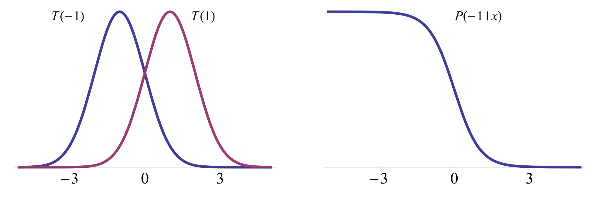
Experiment and Loss Specific Features. Let $\Theta=\{-1,1\}$ with $T(\theta)$ a normal distribution centred on $\theta$ as in the figure below.

For this experiment ,$L_{01}$ and a uniform prior $\pi$, the best decision $d(x)=1$ if $x>0$ as $P(-1|x)>\frac{1}{2}$ and $d(x)=-1$ otherwise as $P(-1|x)\leq\frac{1}{2}$ . It is easy to show that $\Delta\mathcal{V}_{L_{01}}(\pi,d,T)=0$, all we need is the output of $d$. However if we change the loss to a cost sensitive loss $L_{c}$ where say misclassifying a $1$ is more costly than a $-1$, we no longer have $\Delta\mathcal{V}_{L_{c}}(\pi,d,T)=0$.

The reconstruction problem $(X,Z,\phi,X,L_{01})$ that is required to be solved to construct generic features is the most difficult one we can pose. To perform well in this problem we are required to reconstruct each $x\in X$ exactly. This discards other interesting structure the set $X$ may have. For example if $X$ is image data a different loss function $L:X\times X\rightarrow\mathbb{R}$, perhaps one elicited from psychological tests of what humans perceive to be different images is more appropriate. While these are valid points, we remind the reader that this is a first step in understanding these methods, and making any extra assumptions about $X$ and its structure is exactly what we are trying to avoid. However, the Hellman Raviv inequality does give means of bounding the value $\mathcal{V}_{L_{01}}(\pi,\phi)$ with the value of different reconstruction problems.

Lemma Factoring through has the following properties. For all sets $W,X,Y,Z$ and Markov kernels $T_{1}:X\rightsquigarrow Y$ and $T_{2}:Y\rightsquigarrow W$ we have

1. 1.

   $M(X,Z)_{T_{1}}\supseteq M(X,Z)_{T_{2}\circ T_{1}}$

2. 2.

   $M(X,Z)=M(X,Z)_{id_{X}}\supseteq M(X,Z)_{T_{1}}$

3. 3.

   $M(X,Z)_{T_{1}}\supseteq M(X,Z)_{\bullet_{X}}$

Note that $M(X,Z)_{\bullet_{X}}$ comprises the constant Markov kernels, ones that map each $x\in X$ to the same distribution on $Z$.

One can view factoring through as adding noise. By showing that $T|U$, we are showing that $U$ is $T$ composed with extra noise $U/T$

For some intuition on what factoring through looks like below is a plot of four binary experiments ($\Theta={-1,1}$).

We have that:

• •

  The second factors through the first.

• •

  The third does not factor through the first (nor the first through the third).

• •

  The fourth factors through the first and vice versa (it is just a shifted version of the first).

Suppose $T:\Theta\rightsquigarrow X$ and $U:\Theta\rightsquigarrow Y$ are two Markov kernels. If $T|U$ and $U|T$ then we say that $T$ is isomorphic to $U$ written $T\cong U$. Isomorphic Markov kernels can appear quite different. For example suppose that $T:\Theta\rightsquigarrow X$ is an exponential family distribution ($\Theta$ in this case are the parameters for the family). If $\phi:X\rightarrow\mathbb{R}^{n}$ is the sufficient statistics for the family $T$ then $T\cong\phi\circ T$ even though they appear quite different, and that it appears $\phi$ may throw away lots of information. From a statistical point of view isomorphic Markov kernels are the same.

Theorem For all experiments $T$, loss functions $L$ and priors $\pi$, the gap between then the value of $T$ and the least informative experiment $\bullet_{\Theta}$ is a $f$-information for suitable $f$

We repeat the proof presented in Garcia-Garcia and Williamson (2012), which is a variant of one presented in DeGroot (1962).

References

• [1] Arindam Banerjee, Srujana Merugu, Inderjit S. Dhillon, and Joydeep Ghosh. Clustering with Bregman divergences. The Journal of Machine Learning Research, 6:1705–1749, 2005.
• [2] Mikhail Belkin and Partha Niyogi. Laplacian eigenmaps for dimensionality reduction and data representation. Neural computation, 15(6):1373–1396, 2003.
• [3] Anthony J. Bell and Terrence J. Sejnowski. An information-maximization approach to blind separation and blind deconvolution. Neural computation, 7(6):1129–1159, 1995.
• [4] Yoshua Bengio. Learning deep architectures for AI. Foundations and Trends® in Machine Learning, 2(1):1–127, 2009.
• [5] David Blackwell. Comparison of experiments. In Second Berkeley Symposium on Mathematical Statistics and Probability, volume 1, pages 93–102, 1951.
• [6] David Blackwell. Equivalent comparisons of experiments. The Annals of Mathematical Statistics, 24(2):265–272, 1953.
• [7] Thomas M. Cover and Jay A. Thomas. Elements of Information Theory. Wiley, 2012.
• [8] A. Phillip Dawid. The geometry of proper scoring rules. Annals of the Institute of Statistical Mathematics, (April 2006):77–93, 2007.
• [9] Morris H. DeGroot. Uncertainty, information, and sequential experiments. The Annals of Mathematical Statistics, 33(2):404–419, 1962.
• [10] Thomas Shelburne Ferguson. Mathematical statistics: A decision theoretic approach. Academic Press New York, 1967.
• [11] Dario Garcia-Garcia and Robert C. Williamson. Divergences and Risks for Multiclass Experiments. In Conference on Learning Theory (JMLR: W&CP), volume 23, 2012.
• [12] Peter D. Grünwald and A. Philip Dawid. Game theory, maximum entropy, minimum discrepancy and robust Bayesian decision theory. The Annals of Statistics, 32(4):1367–1433, 2004.
• [13] Martin Hellman and Josef Raviv. Probability of error, equivocation, and the Chernoff bound. IEEE Transactions on Information Theory, 16(4):368–372, 1970.
• [14] Geoffrey E. Hinton and Ruslan R. Salakhutdinov. Reducing the dimensionality of data with neural networks. Science, 313(5786):504–507, 2006.
• [15] Peter J. Huber. Robust Statistics. Wiley Series in Probability and Statistics. Wiley, 2011.
• [16] Hidetoshi Komiya. Elementary proof for Sion’s minimax theorem. Kodai mathematical journal, 11(1):5–7, 1988. ISSN 0386-5991.
• [17] Lucien Lecam. Sufficiency and approximate sufficiency. The Annals of Mathematical Statistics, 35(4):1419–1455, 1964.
• [18] Lucien Lecam. On the Information Contained in Additional Observations. The Annals of Statistics, 2(4):630–649, 1974.
• [19] Lucien Lecam. Asymptotic Methods in Statistical Decision Theory. Springer London, 2011.
• [20] Yann LeCun. Learning Representations: A Challenge for Learning Theory, Plenary talk COLT 2013, 2013.
• [21] Honglak Lee, Alexis Battle, Rajat Raina, and Andrew Ng. Efficient sparse coding algorithms. In Advances in neural information processing systems, pages 801–808, 2006.
• [22] Friedrich Liese. phi-divergences, sufficiency, Bayes sufficiency, and deficiency. Kybernetika, 48(4):690–713, 2012.
• [23] Ralph Linsker. An application of the principle of maximum information preservation to linear systems. NIPS, 1989.
• [24] Bruno A. Olshausen and David J. Field. Sparse coding with an overcomplete basis set: A strategy employed by V1? Vision research, 37(23):3311–3325, 1997.
• [25] Matthew Parry, A Philip Dawid, and Steffen Lauritzen. Proper local scoring rules. The Annals of Statistics, 40(1):561–592, 2012.
• [26] Mark D. Reid and Robert C. Williamson. Information, divergence and risk for binary experiments. The Journal of Machine Learning Research, 12:731–817, 2011.
• [27] Vin D. Silva and Joshua B. Tenenbaum. Global versus local methods in nonlinear dimensionality reduction. In Advances in neural information processing systems, pages 705–712, 2002.
• [28] Joshua B. Tenenbaum, Vin De Silva, and John C. Langford. A global geometric framework for nonlinear dimensionality reduction. Science, 290(5500):2319–2323, 2000.
• [29] Naftali Tishby, Fernando C. Pereira, and William Bialek. The information bottleneck method. In Proc. of Allerton Conf. on Communication, Control and Computing, volume physics/00, pages 368–377, 1999.
• [30] Erik Torgersen. Comparison of Statistical Experiments. Cambridge University Press, 1991.
• [31] Pascal Vincent, Hugo Larochelle, Yoshua Bengio, and Pierre-Antoine Manzagol. Extracting and composing robust features with denoising autoencoders. In Proceedings of the 25th International Conference on Machine Learning, pages 1096–1103. ACM, 2008.
• [32] Moshe Zakai and Jacob Ziv. A generalization of the rate-distortion theory and application. Information Theory, New Trends and Open Problems, pages 87–123, 1975.
• [33] Jacob Ziv and Moshe Zakai. On functionals satisfying a data-processing theorem. IEEE Transactions on Information Theory, I(3):770–772, 1973.