Supplementary Material: Learning the Parameters of Determinantal Point Process Kernels
Abstract
Determinantal point processes (DPPs) are well-suited for modeling repulsion and have proven useful in many applications where diversity is desired. While DPPs have many appealing properties, such as efficient sampling, learning the parameters of a DPP is still considered a difficult problem due to the non-convex nature of the likelihood function. In this paper, we propose using Bayesian methods to learn the DPP kernel parameters. These methods are applicable in large-scale and continuous DPP settings even when the exact form of the eigendecomposition is unknown. We demonstrate the utility of our DPP learning methods in studying the progression of diabetic neuropathy based on spatial distribution of nerve fibers, and in studying human perception of diversity in images.
1 Introduction
A determinantal point process (DPP) provides a distribution over configurations of points. The defining characteristic of the DPP is that it is a repulsive point process, which makes it useful for modeling diversity. Recently, DPPs have played an increasingly important role in machine learning and statistics with applications both in the discrete setting—where they are used as a diverse subset selection method [11, 12, 8, 1, 23, 3]— and in the continuous setting for generating point configurations that tend to be spread out[2, 26].
Formally, given a space , a specific point configuration , and a positive semi-definite kernel function , the probability density under a DPP with kernel is given by
| (1) |
where is the matrix with entries for each . This defines a repulsive point process since point configurations that are more spread out according to the metric defined by the kernel have higher densities. To see this, recall that the subdeterminant in Eq. (1) is proportional to the square of the volume spanned by the kernel vectors associated with the points in .
Building on work of Kulesza & Taskar [11], it is intuitive to decompose the kernel as
| (2) |
where can be interpreted as the quality function at point and as the similarity kernel between points and . The ability to bias the quality in certain locations while still maintaining diversity via the similarity kernel offers great modeling flexibility.
One of the remarkable aspects of DPPs is that they offer efficient algorithms for inference, including computing the marginal and conditional probabilities [14], sampling [10, 11, 3, 2], and restricting to fixed-sized point configurations (-DPPs)[12]. However, an important component of DPP modeling, learning the DPP kernel parameters, is still considered a difficult, open problem. Even in the discrete setting, DPP kernel learning has been conjectured to be NP-hard [14]. Intuitively, the issue arises from the fact that in seeking to maximize the log-likelihood of Eq. (1), the numerator yields a concave log-determinant term whereas the normalizer contributes a convex term, leading to a non-convex objective. This non-convexity holds even under various simplifying assumptions on the form of .
Attempts to partially learn the kernel have been studied by, for example, learning the parametric form of the quality function for fixed similarity [13], or learning a weighting on a fixed set of kernel experts [12]. So far, the only attempt to learn the parameters of the similarity kernel has used Nelder-Mead optimization [15], which lacks theoretical guarantees about convergence to a stationary point.
In this paper, we consider parametric forms for the quality function and similarity kernel and propose Bayesian methods to learn the DPP kernel parameters . In addition to capturing posterior uncertainty rather than a single point estimate, these methods can be easily modified to efficiently learn large-scale and continuous DPPs where the eigenstructures are either unknown or are inefficient to compute. In contrast, gradient ascent algorithms for maximum likelihood estimation (MLE) require kernels that are differentiable with respect to in the discrete case. In the continuous case, the eigenvalues must additionally have a known, differentiable functional form, which only occurs in limited scenarios.
In Sec. 2, we review DPPs and their fixed-sized counterpart (-DPPs). We then explore likelihood maximization algorithms for learning DPP and -DPP kernels. After examining the shortcomings of the MLE approach, we propose a set of techniques for Bayesian posterior inference of the kernel parameters in Sec. 3, and explore modifications to accommodate learning large-scale and continuous DPPs. In Sec. 4, we derive a set of DPP moments assuming a known kernel eigenstructure and explore using these moments as a model-checking technique. In low-dimensional settings, we can use a method of moments approach to learn the kernel parameters via numerical techniques. Finally, we test our methods on both simulated and real-world data. Specifically, in Sec. 5 we use DPP learning to study the progression of diabetic neuropathy based on spatial distribution of nerve fibers and also to study human perception of diversity of images.
2 Background
2.1 Discrete DPPs/-DPPs
For a discrete base set , a DPP defined by an positive semi-definite kernel matrix is a probability measure on the possible subsets of :
| (3) |
Here, is the submatrix of indexed by the elements in and is the identity matrix [5].
In many applications, we are instead interested in the probability distribution which gives positive mass only to subsets of a fixed size, . In these cases, we consider fixed-sized DPPs (or -DPPs) with probability distribution on sets of cardinality given by
| (4) |
where are eigenvalues of and is the th elementary symmetric polynomial [12]. Note that can be efficiently computed using recursion [14].
2.2 Continuous DPPs/-DPPs
Consider now the case where is a continuous space. DPPs extend to this case naturally, with now a kernel operator instead of a matrix. Again appealing to Eq. (1), the DPP probability density for point configurations is given by
| (5) |
where are eigenvalues of the operator .
The -DPP also extends to the continuous case with
| (6) |
where .
In contrast to the discrete case, the eigenvalues for continuous DPP kernels are generally unknown; exceptions include a few kernels such as the exponentiated quadratic. However, Affandi et al. [2] showed that a low-rank approximation to can be used to recover an approximation to a finite truncation of the eigenvalues representing an important part of the eigenspectrum. This enables us to approximate the normalizing constants of both DPPs and -DPPs, and will play a crucial role in our proposed methods of Sec. 3.3.
3 Learning Parametric DPPs
Assume that we are given a training set consisting of samples , and that we model these data using a DPP/-DPP with parametric kernel
| (7) |
with parameters . We denote the associated kernel matrix for a set by and the full kernel matrix/operator by . Likewise, we denote the kernel eigenvalues by . In this section, we explore various methods for DPP/-DPP learning.
3.1 Learning using Optimization Methods
To learn the parameters of a discrete DPP model, we can maximize the log-likelihood
| (8) |
Lavancier et al. [15] suggests that the Nelder-Mead simplex algorithm [19] can be used to maximize . This method is based on evaluating the objective function at the vertices of a simplex, then iteratively shrinking the simplex towards an optimal point. While this method is convenient since it does not require explicit knowledge of derivates of , it is regarded as a heuristic search method and is known for its failure to necessarily converge to a stationary point [17].
Gradient ascent and stochastic gradient ascent provide more attractive approaches because of their theoretical guarantees, but require knowledge of the gradient of . In the discrete DPP setting, this gradient can be computed straightforwardly, and we provide examples for discrete Gaussian and polynomial kernels in the Supplementary Material. We note, however, that these methods are still susceptible to convergence to local optima due to the non-convex likelihood landscape.
The log likelihood of the -DPP kernel parameter is
| (9) |
which presents an addition complication due to needing a sum over terms in the gradient.
For continuous DPPs/-DPPs, gradient ascent can only be used in cases where the exact eigendecomposition of the kernel operator is known with a differentiable form for the eigenvalues (see Eq. (5)). This restricts the applicability of gradient-based likelihood maximization to a limited set of scenarios, such as a DPP with Gaussian quality function and similarity kernel. Furthermore, for kernel operators with infinite rank (such as the Gaussian), an explicit truncation has to be made, resulting in an approximate gradient of . Unfortunately, such approximate gradients are not unbiased estimates of the true gradient, so the theory associated with attractive stochastic gradient based approaches does not hold.
3.2 Bayesian Learning for Discrete DPPs
Instead of optimizing the likelihood to get an MLE, here we propose a Bayesian approach to that samples from the posterior distribution over kernel parameters:
| (10) |
for the DPP and, for the -DPP,
| (11) |
Here, is the prior on . Since neither Eq. (10) nor Eq. (11) yield a closed form posterior, we resort to approximate techniques based on Markov chain Monte Carlo (MCMC). We highlight two techniques: random-walk Metropolis-Hastings (MH) and slice sampling, although other MCMC methods can be employed without loss of generality.
In random-walk MH, we use a proposal distribution to generate a candidate value given the current parameters , which are then accepted or rejected with probability where
| (12) |
The proposal distribution is chosen to have mean . The hyperparameters of tune the width of the distribution, determining the average step size. See Alg. 1 of the Supplementary Material.
While random-walk MH can provide a straightforward means of sampling from the posterior, its efficiency requires tuning the proposal distribution. Choosing an aggressive proposal can result in a high rejection rate, while choosing a conservative proposal can result in inefficient exploration of the parameter space. To avoid the need to tune the proposal distribution, we can instead use slice sampling [18], which performs a local search for an acceptable point while still satisfying detailed balance conditions. We first describe this method in the univariate case, following the “linear stepping-out” approach described in Neal [18]. Given the current parameter , we first sample . This defines our slice with all values of with greater than included in the slice. We then define a random interval around with width that is linearly expanded until neither endpoint is in the slice. We propose uniformly in the interval. If is in the slice, it is accepted. Otherwise, becomes the new boundary of the interval, shrinking it so as to still include the current state of the Markov chain. This procedure is repeated until a proposed is accepted. See Alg. 2 of the Supplementary Material.
There are many ways to extend this algorithm to a multidimensional setting. We consider the simplest extension proposed by Neal [18] where we use hyperrectangles instead of intervals. A hyperrectangle region is constructed around and the edge in each dimension is expanded or shrunk depending on whether its endpoints lie inside or outside the slice. One could alternatively consider coordinate-wise or random-direction approaches to multidimensional slice sampling.
As an illustrative example, we consider synthetic data generated from a two-dimensional discrete DPP using a kernel where
| (13) | ||||
| (14) |
where and . We consider to be a grid of 100 points evenly spaced in a unit square and simulate 100 samples from a DPP with kernel as above. We then condition on these simulated data and perform posterior inference of the kernel parameters using MCMC. Fig. 1 shows the sample autocorrelation function of the slowest mixing parameter, , learned using random-walk MH and slice sampling. Furthermore, we ran a Gelman-Rubin test [7] on 5 chains starting from overdispersed starting positions and found that the average partial scale reduction function across the four parameters to be 1.016 for MH and 1.023 for slice sampling, indicating fast mixing of the posterior samples.
3.3 Bayesian Learning for Large-Scale Discrete and Continuous DPPs
In the large-scale discrete or continuous settings, evaluating the normalizers or , respectively, can be inefficient or infeasible. Even in cases where an explicit form of the truncated eigenvalues can be computed, this will only lead to approximate MLE solutions, as discussed in Sec. 3.1.
On the surface, it seems that most MCMC algorithms will suffer from the same problem since they require knowledge of the likelihood as well. However, we argue that for most of these algorithms, an upper and lower bound of the posterior probability is sufficient as long as we can control the accuracy of these bounds. In particular, denote the upper and lower bounds by and , respectively. In the random-walk MH algorithm we can then compute the upper and lower bounds on the acceptance ratio,
| (15) | ||||
| (16) |
We can precompute the threshold , so we can still sometimes accept or reject the proposal even if these bounds have not completely converged. All that is necessary is for (immediately reject) or (immediately accept). In the case that , we can perform further computations to increase the accuracy of our bounds until a decision can be made. As we only sample once in the beginning, this iterative procedure yields a Markov chain with the exact target posterior as its stationary distribution; all we have done is “short-circuit” the computation once we have bounded the acceptance ratio away from . We show this procedure in Alg. 3 of the Supplementary Material.
The same idea applies to slice sampling. In the first step of generating a slice, instead of sampling , we use a rejection sampling scheme first propose a candidate slice as
| (17) |
We then decide whether , in which case we know and we accept as the slice and set . In the case where , we keep increasing the tightness of our bounds until a decision can be made. If at any point exceeds the newly computed , we know that so we reject the proposal. In this case, we generate a new and repeat.
Upon accepting a slice , the subsequent steps for proposing a parameter proceed in a similarly modified manner. For the interval computation, the endpoints are each examined to decide whether (endpoint is not in slice) or (endpoint is in slice). The tightness of the posterior bounds is increased until a decision can be made and the interval can be adjusted, if need be. After convergence of the interval, is generated uniformly over the interval and is likewise tested for acceptance. We illustrate this procedure in Fig. 1 of the Supplementary Material.
The lower and upper bounds of the posterior probability can in fact be incorporated in many MCMC-type algorithms. This provides a convenient and efficient way to garner posterior samples assuming that tightening the bounds can be done efficiently. In our case, the upper and lower bounds for the posterior probability depends on the truncation of the kernel eigenvalues and can be arbitrarily tightened by including more terms in the truncation. In the discrete DPP/-DPP settings, the eigenvalues can be efficiently computed to a specified point using methods such as power law iterations. The corresponding bounds for a Gaussian kernel example are shown in Fig. 2. In the continuous setting, explicit truncation can be done when the kernel has Gaussian quality and similarity, as we show in Sec. 5.1. For other continuous DPP kernels, low-rank approximations can be used [2] resulting in approximate posterior samples. In contrast, a gradient ascent algorithm for MLE is not even feasible: we do not know the form of the approximated eigenvalues, so we cannot take their derivative.
Explicit forms for the posterior probability bounds of for DPPs and -DPPs as a function of the eigenvalue truncations follow from Prop. C.1 and C.2 combined with Eqs. (10) and (11), respectively. Proofs are in the Supplementary Material.
Proposition 3.1
Let be the eigenvalues of kernel . Then
| (18) |
and
| (19) |
Proposition 3.2
Let be the eigenvalues of kernel . Then
| (20) |
and
| (21) |
Finally note that the expression in the bounds can be easily computed as either in the discrete case or in the continuous case.


4 Method of Moments
Convergence and mixing of MCMC samplers can be challenging to assess. Although generic techniques such as Gelman-Rubin diagnostics [7] are applicable, we additionally provide a set of tools more directly tailored to the DPP by deriving a set of theoretical moments. When performing posterior inference of kernel parameters, we can check whether the moments of our data match the theoretical moments given by the posterior samples. This can be done in cases where the eigenstructure is fully known.
In the discrete case, we first need to compute the marginal probabilities. Borodin [4] shows that the marginal kernel, , can be computed directly from :
| (22) |
The th moment can then be calculated via
| (23) |
In the continuous case, given the eigendecomposition of the kernel operator, (where denotes the complex conjugate of the th eigenfunction), the th moment is
| (24) |
Note that this generally cannot be evaluated in closed form since the eigendecompositions of most kernel operators are not known. However, in certain cases where the eigenfunctions are known analytically, the moments can be directly computed. For a kernel defined by Gaussian quality and similarity (see Sec. 5.1), the eigendecomposition can be performed using Hermite polynomials. In the Supplementary Material, we derive the th moment in this setting.
Unfortunately, the method of moments can be challenging to use for direct parameter learning since Eqs. (23) and (39) are not analytically available in most cases. In low dimensions, these quantities can be estimated numerically, but it remains an open question as to how these moments should be estimated for large-scale problems.
5 Experiments
5.1 Simulations
We provide an explicit example of Bayesian learning for a continuous DPP with the kernel defined by
| (25) | ||||
| (26) |
Here, and the eigenvalues of the operator are given by [6],
| (27) |
where , , and is a multi-index.
Furthermore, the trace of can be easily computed as
| (28) |
We test our Bayesian learning algorithms on simulated data generated from a 2-dimensional isotropic kernel (, for ) using Gibbs sampling [2]. We then learn the parameters under weakly informative inverse gamma priors on , and . Details are in the Supplementary Material. We tweak the used for simulation so that we have the following three scenarios:
- (i)
10 DPP samples with average number of points=18 using
- (ii)
1000 DPP samples with average number of points=18 using
- (iii)
10 DPP samples with average number of points=77 using .


Fig. 3 shows trace plots of the posterior samples for all three scenarios. In the first scenario, the parameter estimates vary wildly whereas in the other two scenarios, the posterior estimates are more stable. In all the cases, the zeroth and second moment estimated from the posterior samples are in the neighborhood of the corresponding empirical moments. This leads us to believe that the posterior is broad in cases where we have both a small number of samples and few points in each sample. The posterior becomes more peaked as the total number of points increases. Note that using a stationary similarity kernel allows us to garner information either from few sets with many points or many sets of few points.
Dispersion Measure
In many applications, we are interested in quantifying the overdispersion of point process data. In spatial statistics, one standard quantity used to measure dispersion is the Ripley -function [22]. Here, instead, we would like to use the learned parameters of the DPP to measure overdispersion as repulsion. An important characteristic of a measure of repulsion is that it should be invariant to scaling. In the Supplementary Material, we derive results that, as the data are scaled from to , the parameters scale from to . This suggests that an appropriate scale-invariant measure of repulsion is .
5.2 Applications
5.2.1 Diabetic Neuropathy
Recent breakthroughs in skin tissue imaging have spurred interest in studying the spatial patterns of nerve fibers in diabetic patients. It has been observed that these nerve fibers appear to become more clustered as diabetes progresses. Waller et al. [25] previously analyzed this phenomena based on 6 thigh nerve fiber samples. These samples were collected from 5 diabetic patients at different stages of diabetic neuropathy and one healthy subject. On average, there are 79 points in each sample (see Fig. 4). Waller et al. [25] analyzed the Ripley -function and concluded that the difference between the healthy and severely diabetic samples is highly significant.


We instead study the differences between these samples by learning the kernel parameters of a DPP and quantifying the level of repulsion of the point process. Due to the small sample size, we consider a 2-class study of Normal/Mildly Diabetic versus Moderately/Severely Diabetic. We perform two analyses. In the first, we directly quantify the level of repulsion based on our scale-invariant statistic, (see Sec. 5.1). In the second, we perform a leave-one-out classification by training the parameters on the two classes with one sample left out. We then evaluate the likelihood of the held-out sample under the two learned classes. We repeat this for all six samples.
We model our data using a 2-dimensional continuous DPP with Gaussian quality and similarity as in Eqs. (40) and (41). Since there is no observed preferred direction in the data, we use an isotropic kernel ( and for ). We place weakly informative inverse gamma priors on , as specified in the Supplementary Material, and learn the parameters using slice sampling with eigenvalue bounds as outlined in Sec. 3.3. The results shown in Fig. 5 indicate that our measure clearly separates the two classes, concurring with the results of Waller et al. [25]. Furthermore, we are able to correctly classify all six samples. While the results are preliminary, being based on only six observations, they show promise for this task.


5.2.2 Diversity in Images
We also examine DPP learning for quantifying how visual features relate to human perception of diversity in different image categories. This is useful in applications such as image search, where it is desirable to present users with a set of images that are not only relevant to the query, but diverse as well.
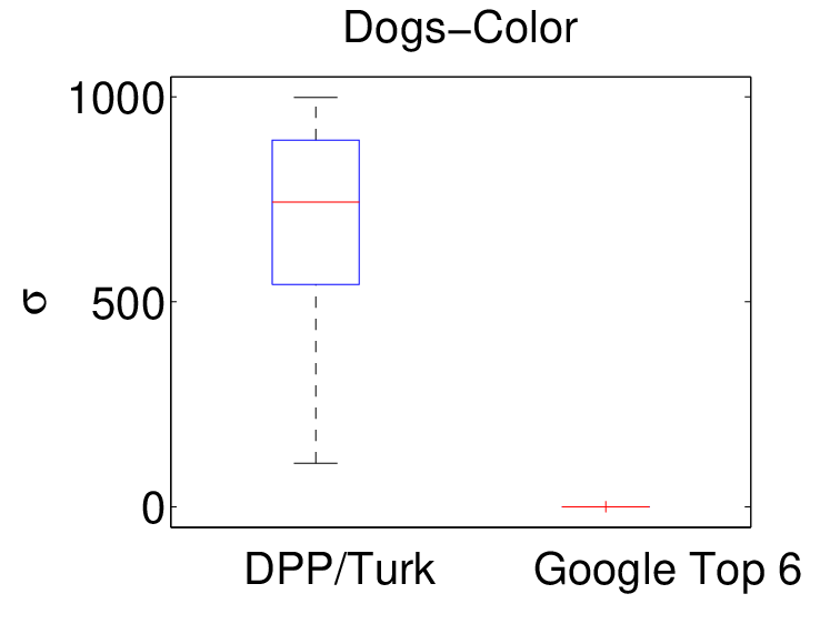
Building on work by Kulesza & Taskar [12], three image categories—cars, dogs and cities—were studied. Within each category, 8-12 subcategories (such as Ford for cars, London for cities and poodle for dogs) were queried from Google Image Search and the top 64 results were retrieved. For a subcategory subcat, these images form our base set . To assess human perception of diversity, human annotated sets of size six were generated from these base sets. However, it is challenging to ask a human to coherently select six diverse images from a set of 64 total. Instead, Kulesza & Taskar [12] generated a partial result set of five images from a 5-DPP on each with a kernel based on the SIFT256 features (see Supplementary Material). Human annotators (via Amazon Mechanical Turk) were then presented with two images selected at random from the remaining subcategory images and asked to add the image they felt was least similar to the partial result set. These experiments resulted in about 500 samples spread evenly spread evenly across the different subcategories.
We aim to study how the human annotated sets differ from the top six Google results, Top-6. As in Kulesza & Taskar [12], we extracted three types of features from the images—color features, SIFT descriptors [24, 16] and GIST descriptors [20] described in the Supplementary Material. We denote these features for image as , , and , respectively. For each subcategory, we model our data as a discrete 6-DPP on with kernel
| (29) |
for and indexing the 64 images in . Here, we assume that each category has the same parameters across subcategories, namely, for and .
To learn from the Top-6 images, we consider the samples as being generated from a 6-DPP. To emphasize the human component of the 5-DPP + human annotation sets, we examine a conditional 6-DPP [14] that fixes the five images from the partial results set and only considers the probability of adding the human annotated image. The Supplementary Material provides details on this conditional -DPP.
All subcategory samples within a category are assumed to be independent draws from a DPP defined on with kernel parameterized by a shared set of , for . As such, each of these samples equally informs the posterior of . We perform posterior sampling of the 6-DPP or conditional 6-DPP kernel parameters using slice sampling with weakly informative inverse gamma priors on the . Details are in the Supplementary Material.
Fig. 6 shows a comparison between learned from the human annotated samples (conditioning on the 5-DPP partial result sets) and the Top-6 samples for different categories. The results indicate that the 5-DPP + human annotated samples differs significantly from the Top-6 samples in the features judged by human to be important in diversity in each category. For cars and dogs, human annotators deem color to be a more important feature for diversity than the Google search engine based on their Top-6 results. For cities, on the other hand, the SIFT features are deemed important for diversity by human annotators, while the Google search engine puts a much lower weight on them. Keep in mind, though, that this result only highlights the diversity components of the results while ignoring quality. In real life applications, it is desirable to combine both the quality of each image (as a measure of relevance of the image to the query) and the diversity between the top results. Regardless, we have shown that DPP kernel learning can be informative of judgements of diversity, and this information could be used (for example) to tune search engines to provide results more in accordance with human judgement.
6 Conclusion
Determinantal point processes have become increasingly popular in machine learning and statistics. While many important DPP computations are efficient, learning the parameters of a DPP kernel is difficult due to the non-convexity of the likelihood. We proposed Bayesian approaches using MCMC, in particular, for inferring these parameters. In addition to being more robust and providing a characterization of the posterior uncertainty, these algorithms can be modified to deal with large-scale and continuous DPPs. We also showed how our posterior samples can be evaluated using moment matching as a model-checking method. Finally we demonstrated the utility of learning DPP parameters in studying diabetic neuropathy and evaluating human perception of diversity in images.




References
- [1] Affandi, R. H., Kulesza, A., and Fox, E. B. Markov determinantal point processes. In Proc. UAI, 2012.
- [2] Affandi, R. H., Fox, E.B., and Taskar, B. Approximate inference in continuous determinantal processes. In Proc. NIPS, 2013a.
- [3] Affandi, R.H., Kulesza, A., Fox, E.B., and Taskar, B. Nyström approximation for large-scale determinantal processes. In Proc. AISTATS, 2013b.
- [4] Borodin, A. Determinantal point processes. arXiv preprint arXiv:0911.1153, 2009.
- [5] Borodin, A. and Rains, E.M. Eynard-Mehta theorem, Schur process, and their Pfaffian analogs. Journal of statistical physics, 121(3):291–317, 2005.
- [6] Fasshauer, G.E. and McCourt, M.J. Stable evaluation of Gaussian radial basis function interpolants. SIAM Journal on Scientific Computing, 34(2):737–762, 2012.
- [7] Gelman, A. and Rubin, D. B. Inference from iterative simulation using multiple sequences. Statistical science, pp. 457–472, 1992.
- [8] Gillenwater, J., Kulesza, A., and Taskar, B. Discovering diverse and salient threads in document collections. In Proc. EMNLP, 2012.
- [9] Guan, K. Schur-convexity of the complete elementary symmetric function. Journal of Inequalities and Applications, 2006(1):67624, 2006.
- [10] Hough, J.B., Krishnapur, M., Peres, Y., and Virág, B. Determinantal processes and independence. Probability Surveys, 3:206–229, 2006.
- [11] Kulesza, A. and Taskar, B. Structured determinantal point processes. In Proc. NIPS, 2010.
- [12] Kulesza, A. and Taskar, B. k-DPPs: Fixed-size determinantal point processes. In ICML, 2011a.
- [13] Kulesza, A. and Taskar, B. Learning determinantal point processes. In In Proc. UAI, 2011b.
- [14] Kulesza, A. and Taskar, B. Determinantal point processes for machine learning. Foundations and Trends in Machine Learning, 5(2–3), 2012.
- [15] Lavancier, F., Møller, J., and Rubak, E. Statistical aspects of determinantal point processes. arXiv preprint arXiv:1205.4818, 2012.
- [16] Lowe, D. G. Object recognition from local scale-invariant features. In Computer vision, 1999. The proceedings of the seventh IEEE international conference on, volume 2, pp. 1150–1157. Ieee, 1999.
- [17] McKinnon, K. I.M. Convergence of the Nelder–Mead simplex method to a nonstationary point. SIAM Journal on Optimization, 9(1):148–158, 1998.
- [18] Neal, R. M. Slice sampling. Annals of statistics, pp. 705–741, 2003.
- [19] Nelder, J. and Mead, R. A simplex method for function minimization. Computer Journal, 7(4):308–313, 1965.
- [20] Oliva, A. and Torralba, A. Building the gist of a scene: The role of global image features in recognition. Progress in brain research, 155:23–36, 2006.
- [21] Paris, R.B. Asymptotics of integrals of hermite polynomials. Appl. Math. Sci. 4, pp. 3043–3056, 2010.
- [22] Ripley, B. D. Modelling spatial patterns. Journal of the Royal Statistical Society. Series B (Methodological), pp. 172–212, 1977.
- [23] Snoek, J., Zemel, R., and Adams, R. P. A determinantal point process latent variable model for inhibition in neural spiking data. In Proc. NIPS, 2013.
- [24] Vedaldi, A. and Fulkerson, B. Vlfeat: An open and portable library of computer vision algorithms. In Proceedings of the international conference on Multimedia, pp. 1469–1472. ACM, 2010.
- [25] Waller, L. A., Särkkä, A., Olsbo, V., Myllymäki, M., Panoutsopoulou, I.G., Kennedy, W.R., and Wendelschafer-Crabb, G. Second-order spatial analysis of epidermal nerve fibers. Statistics in Medicine, 30(23):2827–2841, 2011.
- [26] Zou, J. and Adams, R.P. Priors for diversity in generative latent variable models. In Proc. NIPS, 2012.
Appendix A Gradient for Discrete DPP
Gradient ascent and stochastic gradient ascent provide attractive approaches in learning parameters, of DPP kernel because of their theoretical guarantees, but require knowledge of the gradient of the log-likelihood . In the discrete DPP setting, this gradient can be computed straightforwardly and we provide examples for discrete Gaussian and polynomial kernels here.
| (30) |
To find the MLE, we can perform gradient ascent
| (31) |
In the following examples, we denote
, where is the number of dimension.
A.1 Example I: Gaussian Similarity with Uniform Quality
Denote
Then,
A.2 Example II: Gaussian Similarity with Gaussian Quality
Denote and as in previous example.
Then,
and is the same as the previous example.
A.3 Example III: Polynomial Similarity with Uniform Quality
Denote and .
Then,
Appendix B Bayesian Learning
In the main paper, we highlight two techniques: random-walk Metropolis-Hastings (MH) and slice sampling to sample from the posterior distribution. We present the pseudo algorithms here (Alg. 1 and Alg. 2).
We also present the pseudo random walk MH algorithm for handling large-scale and continuous DPPs using posterior bounds in Alg. 3. We also present and illustration of the slice sampling using posterior bounds in Figure 7.

Appendix C Proof of DPP/DPP Bounds
Proposition C.1
Let be the eigenvalues of kernel . Then
| (32) |
and
| (33) |
Proof: The first inequality is trivial since the eigenvalues are all nonnegative.
To proof the second inequality, we use the AM-GM inequality: For any non-negative numbers, .
Let and . Then,
Proposition C.2
Let be the eigenvalues of kernel . Then
| (34) |
and
| (35) |
Proof: Let be the th elementary symmetric function:
Trivially, we have a lower bound since the eigenvalues are non-negative:
For the upper bound we can use the Schur-concavity of elementary symmetric functions for non-negative arguments [9].Thus for :
| (36) |
and
| (37) |
we have .
Now let and . We consider
| (38) |
Note that and so for .
We now compute . Note that for , the terms in the sum are products of factors, each containing some of the factors and some of the factors. The sum of the terms that have factors of type is , so we have:
Using , we get
Letting , we get out upper bound
Appendix D Moments for Continuous DPP with Gaussian Quality and Similarity
In the continuous case, given the eigendecomposition of the kernel operator, (where denotes the complex conjugate of the th eigenfunction), the th moment can be evaluated as
| (39) |
Here we present the derivation for moments when
| (40) |
and
| (41) |
In this case, the eigenvalues and eigenvectors of the operator are given by Fasshauer & McCourt [6],
| (42) |
and
| (43) |
where , and is a multi index.
In the case of DPPs (as opposed to -DPPs), we can use the number of items as an estimate of the 0th moment. The 0th moment is given by . Denote . The for higher moments, note that
Using the results of moment integrals involving a product of two Hermite polynomials [21], we get that
| (44) |
for even and 0 otherwise. The polynomial is given in Eq. (4.8) in Paris [21]. For example, the second and fourth moments are given by
- (i)
- (ii)
For a low dimensional setting, we can learn the parameters by using grid search such that the moments agree.
Appendix E Details on Simulation
In the main paper, we use our Bayesian learning algorithms to learn parameters from (i) simulated data generated from a 2-dimensional isotropic discrete kernel (, for ), (ii) nerve fiber data using 2-dimensional isotropic continuous kernel (, for ) and (ii) image diversity data using 3600-dimensional discrete kernel with Gaussian similarity. In all of these experiments, we use weakly informative inverse gamma priors on , and . In particular, for all three parameters, we used the same priors for all three parameters
| (45) |
We then learn the parameters using hyperrectangle slice sampling.
Appendix F Details on Image Diversity
In studying the diversity in images, we extracted 3 different types of features from the images—color features, SIFT-descriptors [16, 24] and GIST-descriptors [20] described in the supplementary material. We describe these features below.
Color: Each pixel is assigned a coordinate in three-dimensional Lab color space. The colors are then sorted into axis-aligned bins, producing a histogram of either 8 (denoted color8) or 64 (denoted color64) dimensions.
SIFT: The images are processed to obtain sets of 128-dimensional SIFT descriptors. These descriptors are commonly used in object recognition to identify objects in images and are invariant to scaling, orientation and minor distortions. The descriptors for a given category are combined, subsampled to set of 25,000, and then clustered using k-means into either 256 (denoted SIFT256) or 512 (denoted SIFT512) clusters. The feature vector for an image is the normalized histogram of the nearest clusters to the descriptors in the image.
GIST: The images are processed to obtain 960-dimensional GIST feature vectors that is commonly used to describe scene structure.
We also extracted the features above from the center of the images, defined as the centered rectangle with dimensions half those of the original image. This yields a total of 10 different feature vectors. Since we are only concerned with the diversity of the images, we ensure that the quality across the images are uniform by normalizing each feature vector such that their norm equals to 1. We then combine the feature vectors into 3 types of features- color, SIFT and GIST.
For the Google top 6 images, we model the samples, as though they are generated from a 6-DPP with kernel . To highlight the effect of the human annotation in the partial results sets, we model the samples as though they are generated from a conditional 6-DPP.
In general, given a partial set of observations A and -DPP kernel , we can define the conditional -DPP probability of choosing a set B given the inclusion of set A (with )as
| (46) |
with
| (47) |
where denotes the identity matrix with 0 for diagonal corresponding to elements in . Here, following the inversion, the matrix is restricted to rows and columns indexed by elements not in , then inverted again. The normalizer is given by Kulesza & Taskar [14].
| (48) |
In our experiment, our samples can be seperated into the partial result sets and human annotations,
| (49) |
where is the partial result sets and is the human annotated result, we model the data from the conditional -DPP . In this case, the likelihood is given by
| (50) |
for each subcategory, . That is, for each subcategory, i, we compute and use Eq. 47 to compute the conditional kernel.