Suppression of Geometric Barrier in Type II Superconducting Strips

R. Willa Affiliation: Institute for Theoretical Physics, ETH Zurich, 8093 Zurich, Switzerland V.B. Geshkenbein Affiliation: Institute for Theoretical Physics, ETH Zurich, 8093 Zurich, Switzerland G. Blatter Affiliation: Institute for Theoretical Physics, ETH Zurich, 8093 Zurich, Switzerland

August 24, 2026

Abstract

We study the magnetic response of a superconducting double strip, i.e., two parallel coplanar thin strips of width $2w$ , thickness $d\ll w$ and of infinite length, separated by a gap of width $2s$ and subject to a perpendicular magnetic field $H$ . The magnetic properties of this system are governed by the presence of a geometric energy barrier for vortex penetration which we investigate as a function of applied field $H$ and gap parameter $s$ . The new results deal with the case of a narrow gap $s\ll w$ , where the field penetration from the inner edges is facilitated by large flux focusing. Upon reducing the gap width $2s$ , we observe a considerable rearrangement of the screening currents, leading to a strong reduction of the penetration field and the overall magnetization loop, with a suppression factor reaching $\sim(d/w)^{1/2}$ as the gap drops below the sample thickness, $2s<d$ . We compare our results with similar systems of different shapes (elliptic, rectangular platelet) and include effects of surface barriers as well. Furthermore, we verify that corrections arising from the magnetic response of the Shubnikov phase in the penetrated state are small and can be omitted. Extending the analysis to multiple strips, we determine the specific sequence of flux penetrations into the different strips. Our studies are relevant for the understanding of platelet shaped samples with cracks or the penetration into layered superconductors at oblique magnetic fields.

pacs

74.25.Ha, 74.25.Wx, 75.70.-i

I Introduction

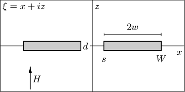
The characteristic properties of a superconductor are its diamagnetic response [1] $M$ to an external magnetic field $H$ and its ability to transport electric current without dissipation[2]. In the Meissner phase the magnetic induction $B=H+4\pi M$ vanishes inside the superconductor and the linear response $M=-H/4\pi$ is that of a perfect (bulk) diamagnet. In type II superconductors, a sufficiently large magnetic field $H>H_{p}$ penetrates the material via quantized flux lines (with flux $\Phi_{0}=hc/2e$ ); we denote with $H_{p}$ the field of first penetration. Within the mixed (or Shubnikov[3]) phase the presence of vortices reduces the bulk diamagnetic signal and the magnetization $M(H)$ decreases in magnitude. The magnetic properties of the material then depend on the behavior of the vortex state. In this paper, we determine the magnetic response of superconducting samples of more complex shape, in particular a double strip, two parallel coplanar thin strips of infinite length and subject to a perpendicular magnetic field $H$ , see Fig. 1. The response of such a system is hysteretic and dominated by the so-called geometrical barrier[4, 5], i.e., an energy barrier retarding the magnetic field penetration. Our main result is an apparent suppression of the geometrical barrier for the situation where the two strips are closeby, i.e., separated by a narrow gap or crack. Such a suppression of geometrical barriers may be of practical interest in experiments, as has been the case in disentangling the vortex lattice melting- and irreversibility lines in layered BiSCCO superconductors [6] or in separating apart the phenomenon of bulk vortex pinning by defects. So far, the geometrical barrier has been deliberately suppressed by polishing the sample into the shape of a prism [6]; the suppression of the geometrical barrier observed when tilting the magnetic field applied to the sample [7] and attributed to the appearance of Josephson vortex stacks resembles the mechanism reported in the present paper.

Refer to caption — Figure 1: Side-view representation ( $xz$ -plane) of two flat superconducting strips (parallel to $y$ ) subject to a perpendicular magnetic field $H$ (directed along $z$ ). The cross-sections of the strips have a width $2w$ and a thickness $d\ll w$ , while the separation $2s$ between their inner edges measures the width of the gap. The outer edges of the strips at $\pm(2w+s)$ are denoted by $\pm W$ . Any position in the $xz$ -plane is described by the complex coordinate $\xi=x+iz$ .

The precise shape of the magnetization curve depends on the specific configuration assumed by the vortices after penetration, which is determined by the sample shape and its surface properties (we assume a sample free of defects). The sample surface is relevant in the determination of the penetration field $H_{p}$ as defined in the asymptotic region far away from the sample. A flat surface parallel to the field generates an image vortex which results in a surface barrier hindering vortices from entering the sample [8, 9]. The metastable Meissner state survives until the local field at the surface is increased beyond the critical value $H_{s}$ which is of the order of the thermodynamic critical field $H_{c}$ , $H_{s}\sim H_{c}>H_{c1}$ , with $H_{c1}$ the lower critical field. For a non-ideal surface the effective surface barrier is reduced and assumes a value $H_{s}$ between $H_{c1}$ and $H_{c}$ .

The sample shape is relevant, too, in the determination of the penetration field $H_{p}$ . This is well known for elliptic-shaped samples, cf. Fig. 2, where the magnetic field is enhanced near the sample edge: for a cylindrical shaped diamagnetic (i.e., $\mu=0$ ) sample with an elliptic cross section of height $d$ and width $2w$ , the demagnetization factor[10] $n=2w/(2w+d)$ generates a field enhancement $H_{\mathrm{edge}}=(1-n)^{-1}H$ . Correspondingly, the penetration field is given by $H_{p}=(1-n)H_{s}=d/(2w+d)H_{s}$ . Once the penetration field is reached, vortices enter the sample, reversibly in the absence of a surface barrier (i.e., if $H_{s}=H_{c1}$ ) and irreversibly else. Without surface barrier, the vortices distribute homogeneously inside the sample, a result that is consistent with the constant induction inside a magnetic ellipsoid[11]. On a microscopic level, this corresponds to an exact matching of the energy gain of vortex motion in the field of the screening current and the energy cost $\varepsilon_{l}$ associated with the increasing vortex length upon penetration, see Fig. 2.

For a platelet shaped sample (of width $2w$ and thickness $d$ ) with a rectangular edge, the field at the boundary is enhanced as well, although (effectively) less than for the elliptic sample. A distance $d$ away from the edge[12], the applied field $H$ is enhanced by a factor $\sim(w/d)^{1/2}$ , resulting in a penetration field $H_{p}\sim(d/w)^{1/2}H_{s}$ . At this field strength, the barrier for vortex entry into the sample has vanished and vortices move to the center of the sample where they accumulate in a dome-shaped form, cf. Fig. 2. Under further increase of the external field $H$ , the vortex dome grows both in height and width until the sample is fully penetrated. In this geometry, the cost $\varepsilon_{l}d$ to create the vortex is payed right upon vortex entry at the sample edge; beyond the edge region the energy gain in the current field $I(x)$ is no longer balanced by the energy cost and the vortex is driven to the sample center. Hence the field penetration into the platelet shaped sample is irreversible even in the absence of a surface barrier, what is due to the presence of a geometric barrier defined through the energy cost for flux entry. It is this type of geometric barrier effects [4, 5] which is at the focus of the present paper.

Another situation arises in dirty samples where vortices are pinned onto defects. Once the surface and geometrical barriers are overcome, the vortex arrangement may be dominated by bulk pinning and the magnetic induction (or magnetization) is given by a Bean profile[13]. What is common to all three cases, surface-, geometric-, and bulk pinning is the irreversible, hysteretic behavior of the magnetization $M(H)$ with changing external field $H$ . In this paper, we concentrate on the defect-free case and thus ignore possible modifications due to bulk pinning.

The motivation to study geometrical barriers in samples of complex shape is manifold: Originally, the understanding of the flux penetration and vortex lattice melting in layered high- $T_{c}$ superconductors necessitated a proper analysis of the vortex state in platelet-shaped samples[4]. On the technological side, the structuring of current-carrying strips [14, 15] enhances their critical current as the incorporation of slits generates geometrical barriers hindering vortex motion. Recently, Segev et al.[7] observed a structured vortex dome in layered $\mathrm{Bi_{2}Sr_{2}CaCu_{2}O_{8+\delta}}$ samples subject to a tilted magnetic field. This finding can be interpreted as arising from stacks of in-plane (Josephson) vortices reducing the superconducting order parameter[16] and acting as weak links for the perpendicular field (pancake vortices[17, 18]). Our analysis of vortex penetration into a double-strip with a narrow gap, see Fig. 1, may serve as a first step towards the understanding of flux penetration in this geometry.

From a general perspective, the magnetic response associated with superconducting samples can be calculated numerically. Effects of complex sample shapes, inhomogeneous material equations, and time-dependent perturbations can then be studied quantitatively[19]. On the other hand, analytic approaches give more qualitative insights into the system’s behavior. Earlier work on geometrical barriers in samples with more complex shapes considered the case of two coplanar thin strips in the Meissner phase[20] and the full magnetization curve for a strip-shaped sample with a slit[21], i.e., two strips shunted at their ends; this ring-type topology with circulating currents exhibits a markedly different magnetization $M(H)$ as compared to our unshunted situation. The situation of an unshunted double stripline in the critical state was investigated in Ref. [22]. In our work, we go beyond these results in various ways, including the situation where the sample thickness $d$ plays an important role.

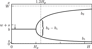
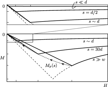
The most pertinent new result is the dramatic suppression of the geometrical barrier which we illustrate in Fig. 3. This suppression is driven by a large flux-focussing into the gap between the strips, forcing the flux penetration into the sample to start from the inner edges. In tracing the evolution of the penetration field $H_{p}$ as a function of separation $s$ between the strips, we find it decay from $H_{p}\sim\sqrt{d/w}\,H_{s}$ at large $s$ to $H_{p}\sim\sqrt{sd/w^{2}}\log(w/s)\,H_{s}$ at intermediate separation $d<s<w$ to $H_{p}\sim(d/w)\,H_{s}$ at small $s\ll d$ ; the latter coincides with the result for the elliptic sample where the geometrical barrier is absent alltogether. We emphasize, however, that the narrow-gap double-strip still differs from the ellipse as the geometrical barrier remains present but rapidly collapses from $\varepsilon_{l}d$ to zero with increasing field, hence maintaining the hysteretic magnetization. The latter strongly decreases with the separation $s$ between strips as well: Within the individual strips, the penetrated field assumes a dome-like shape which is increasingly skewed towards the gap when $s$ becomes small. Following the change in shape of the magnetization curve through the various regimes, we find it to shrink by a factor $\propto(s/w)^{1/2}\log(w/s)$ when $s<w$ and by a factor $\propto(d/w)^{1/2}$ for narrow gaps $s\ll d$ when compared to the single platelet sample; this decay of the magnetization with decreasing $s$ ends up in a flat and nearly constant value $M=-(H_{s}/4\pi)(4wd)$ at small $s\log(W/s)\ll d$ .

In the following, we briefly recall the key features of the magnetic response for elliptically shaped strips in Sec. II.1 and proceed with the description of coplanar parallel rectangular strips for the case where the thickness $d$ is the smallest geometric length in the problem (Sec. II.2). We review the appearance and consequences of a geometric barrier in a single strip (Sec. II.3) and continue with the analysis of two adjacent strips (Sec. II.4) discussing the behavior of the Meissner- and penetrated states. In Sec. III, we analyze the double strip for the situation where the separation $2s$ between the strips is smaller than the strip thickness $d$ , $s\ll d$ . Section IV is devoted to multi-strips and a summary and conclusions are given in Sec. V.

II Thin Strips

II.1 Introduction - Elliptical strip

Before considering samples with rectangular geometries, it is instructive to revisit the magnetic properties of a flat superconducting strip with an elliptic cross-section. The strip extends infinitely in the $y$ -direction and the semi-axes along $x$ and $z$ are $w$ and $d/2$ ( $d\ll w$ ) respectively, with the upper/lower sample surface parametrized by $z_{\pm}(x)=\pm(d/2w)\sqrt{w^{2}-x^{2}}$ . The magnetic field $H$ is applied parallel to the $z$ -axis; outside the sample, $\boldsymbol{B}=\boldsymbol{H}$ , while $B_{\mathrm{el}}=\mu(B_{\mathrm{el}})H_{\mathrm{el}}$ is constant and parallel to the $z$ -axis inside the elliptic sample[11], a consequence of the special elliptic shape. Here,

\displaystyle\mu(B)=\frac{B}{4\pi}\Big(\frac{dF}{dB}\Big)^{-1}

(1)

is the magnetic permeability of the material as obtained from the free energy density $F(B)$ . The magnetic field at the sample edges $(\pm w,0)$ is continuous[11], $H_{\mathrm{el}}=H_{\mathrm{edge}}$ , where $H_{\mathrm{edge}}$ denotes the magnetic field strength at the sample edge. The latter is modified due to demagnetization effects of the sample which are described by the geometric demagnetizing factor[10] $n=2w/(2w+d)\approx 1-d/2w$ . Exploiting the fact that the magnetic induction $B_{\mathrm{el}}$ is constant within the ellipse, we decompose the total field $\boldsymbol{B}(x,z)$ into two components, a constant one $\boldsymbol{B}_{\mathrm{el}}=(0,0,B_{\mathrm{el}})$ , and the remaining field $\boldsymbol{B}_{0}(x,z)$ which does not penetrate the sample. Far away from the sample, all fields point along $z$ , $\boldsymbol{B}_{0}\equiv(0,0,B_{0}^{\infty})$ and we have $B_{\mathrm{el}}+B_{0}^{\infty}=H$ . The component $\boldsymbol{B}_{0}(x,z)$ then describes the field of a perfectly diamagnetic ellipse in the reduced external field $B_{0}^{\infty}=H-B_{\mathrm{el}}$ . The magnetic field at the sample edge ( $x=\pm w$ ) points along $z$ , involves the two components $B_{\mathrm{el}}$ and $B_{0}=B_{0}^{\infty}/(1-n)$ , the latter enhanced by demagnetization effects, and reads

\displaystyle H_{\mathrm{edge}}

\displaystyle=B_{\mathrm{el}}+\frac{B_{0}^{\infty}}{1-n}.

(2)

Using $B_{0}^{\infty}=H-B_{\mathrm{el}}$ as well as $B_{\mathrm{el}}=\mu(B_{\mathrm{el}})H_{\mathrm{el}}=\mu(B_{\mathrm{el}})H_{\mathrm{edge}}$ , we obtain the standard formula for the field strength inside the sample[11]

\displaystyle B_{\mathrm{el}}=\frac{\mu(B_{\mathrm{el}})}{1-n[1-\mu(B_{\mathrm{el}})]}H,

(3)

where the value for $B_{\mathrm{el}}$ has to be determined self-consistently. For notational simplicity we denote by $\mu$ the value for $\mu(B_{\mathrm{el}})$ after solving the above equation.

The $\boldsymbol{B}$ -field at the surface outside of the ellipse has both a normal ( $\perp$ ) and a tangential ( $\|$ ) component. Their magnitudes can be determined from the boundary conditions[11], telling that $B_{\perp}$ and $B_{\|}/\mu$ are continuous across the surface. For the upper surface $z=z_{+}(x)$ of the ellipse we find

\displaystyle\boldsymbol{(}B_{\|}(x),B_{\perp}(x)\boldsymbol{)}

\displaystyle=\frac{H}{1-n(1-\mu)}\boldsymbol{(}\sin(\alpha),\mu\cos(\alpha)\boldsymbol{)},

(4)

where

\displaystyle\alpha(x)

\displaystyle=\arctan\bigg(\frac{d}{2w}\frac{-x}{\sqrt{w^{2}-x^{2}}}\bigg)

(5)

measures the angle between the external field orientation ( $z$ -axis) and the direction normal to the elliptic surface at the position $\boldsymbol{(}x,z_{+}(x)\boldsymbol{)}$ . In most of the strip region (when $w-|x|\gg d^{2}/w$ ) the surface of the ellipse is almost parallel to the $x$ -axis and the above field expression (4) simplifies to

\displaystyle\boldsymbol{(}B_{\|}(x),B_{\perp}(x)\boldsymbol{)}

\displaystyle\approx\frac{H}{1-n(1-\mu)}\Big(\frac{-x(1-n)}{\sqrt{w^{2}-x^{2}}},\mu\Big).

(6)

The discontinuity of the field parallel to the boundary determines the surface current that generates the magnetization of the sample. Using Ampère’s law and defining the sheet current density $I(x)=\int_{z_{-}}^{z_{+}}dz\,j(x,z)$ across the sample, we find

$\displaystyle I(x)$	$\displaystyle\approx\frac{2c}{4\pi}\big[B_{\\|}(x)-B_{\mathrm{el}}\sin(\alpha)\big]$	(7)
	$\displaystyle\approx-\frac{Hc}{2\pi}\frac{(1-n)(1-\mu)}{1-n(1-\mu)}\frac{x}{\sqrt{w^{2}-x^{2}}}$	(8)
	$\displaystyle=-\frac{(H-B_{\mathrm{el}})c}{2\pi}\frac{x}{\sqrt{w^{2}-x^{2}}}.$	(9)

The factor 2 originates from the two current contributions at the upper and lower sample surface. The last expression shows that only the expelled component $B_{0}^{\infty}=H-B_{\mathrm{el}}$ contributes to the shielding currents. The magnetization $M$ (per unit length) is obtained from the relation $4\pi M/A=B_{\mathrm{el}}-H_{\mathrm{el}}$ , where $A=\pi wd/2$ is the area of the strip’s cross-section. Using $H_{\mathrm{el}}=H_{\mathrm{edge}}$ and Eq. (2) gives for the magnetization

\displaystyle M

\displaystyle=-\frac{B_{0}^{\infty}}{4}w^{2}=-\frac{H}{4}\frac{(1-n)(1-\mu)}{1-n(1-\mu)}w^{2}.

(10)

In the last equality we used $B_{0}^{\infty}=H-B_{\mathrm{el}}$ and Eq. (3).

II.1.1 Meissner state

At low fields, the superconducting elliptic strip remains in the Meissner state ( $\mu=0$ ), resulting in a vanishing induction, i.e., $B_{\mathrm{el}}=B=0$ . The field strength at the edge, see Eq. (2), is enhanced by the geometric factor $1/(1-n)\approx 2w/d$ as compared to the applied field $H$ . At the sample surface, the field is everywhere tangential and its strength is given by $H\sin(\alpha)/(1-n)$ $(\approx-Hx/\sqrt{w^{2}-x^{2}})$ as obtained from Eqs. (4) and (6). The resulting sheet current density inside the sample is obtained from Eq. (9),

\displaystyle I(x)

\displaystyle\approx-\frac{Hc}{2\pi}\frac{x}{\sqrt{w^{2}-x^{2}}}.

(11)

The perfectly diamagnetic response [Eq. (10) with $\mu=0$ ]

\displaystyle M

\displaystyle=-\frac{H}{4}w^{2}.

(12)

lasts until the magnetic flux starts penetrating the superconducting sample in the form of vortices.

To bring a vortex to the position $x$ inside the sample costs an energy $U_{\scriptscriptstyle{L}}(x)=\varepsilon_{l}\ell(x)$ , gradually rising with the vortex length $\ell(x)=z_{+}(x)-z_{-}(x)$ from zero at the sample edges to $d$ in the sample center; here, the line-energy $\varepsilon_{l}=\varepsilon_{0}\log(\lambda/\xi)=\Phi_{0}(dF/dB)|_{B=0}$ is the cost per unit length associated with the nucleation of a single vortex in the bulk superconductor. On the other hand, the work gained from the Lorentz force [due to the current $I(x)$ in Eq. (11)] drives the vortex entrance. The two energy contributions can be combined to an effective potential landscape[23] for a single vortex

\displaystyle U_{\mathrm{geo}}(x)

\displaystyle=U_{\scriptscriptstyle{L}}(x)-\frac{\Phi_{0}}{c}\int\limits_{w}^{x}du\,I(u).

(13)

In the elliptical geometry, the functional form of the driving energy due to the current Eq. (11) coincides with the geometrical thickness $\ell(x)=d\sqrt{1-x^{2}/w^{2}}$ of the sample and the energy profile (13) reduces to

\displaystyle U_{\mathrm{geo}}(x)

\displaystyle=\varepsilon_{l}\ell(x)\bigg(1-\frac{H\Phi_{0}}{4\pi\varepsilon_{l}}\frac{2w}{d}\bigg).

(14)

The barrier then vanishes throughout the sample at the penetration field

\displaystyle H_{p}

\displaystyle=\frac{4\pi\varepsilon_{l}}{\Phi_{0}}\frac{d}{2w}=H_{c1}\frac{d}{2w}

(15)

where the local field strength at the edge reaches $H_{c1}$ and the magnetization (per unit length) as obtained from Eq. (12) amounts to

\displaystyle M_{p}=-\frac{H_{c1}}{8}wd=-\frac{H_{c1}}{4\pi}\frac{\pi wd}{2},

(16)

with $\pi wd/2$ the cross-section of the strip.

II.1.2 Penetrated state

Beyond the field of first penetration $H_{p}$ , vortices homogeneously flood the sample, and the potential landscape takes the form (we replace $B_{\mathrm{el}}\to B$ )

\displaystyle U_{\mathrm{geo}}(x)

\displaystyle=\varepsilon_{l}(B)\frac{d}{w}\sqrt{w^{2}-x^{2}}-\frac{\Phi_{0}}{c}\int\limits_{w}^{x}du\,I(u).

(17)

The line energy $\varepsilon_{l}(B)$ describes the energy difference (per unit length) between the vortex state and the homogeneous field configuration, i.e.,

\displaystyle\varepsilon_{l}(B)

\displaystyle=\Phi_{0}\frac{d}{dB}\bigg[F(B)-\frac{B^{2}}{8\pi}\bigg]=\frac{\Phi_{0}B}{4\pi}\frac{1-\mu(B)}{\mu(B)}

(18)

with $F(B)$ the free energy density of the superconducting state. The second term on the right-hand side of Eq. (17) is modified as well, since only the non-penetrating (diamagnetic) part $H-B$ of the field drives the diamagnetic currents in Eq. (9). The resulting state remains in equilibrium for all $H>H_{p}$ , i.e., $U_{\mathrm{geo}}(x)\equiv 0$ , and the reversible magnetic response follows the form in Eq. (10)

\displaystyle M

\displaystyle=-\frac{H-B}{4}w^{2}

(19)

with $B$ determined by the self-consistency equation (3). A finite surface barrier as discussed further below will retard the vortex penetration and generate a hysteretic response.

In order to illustrate the above results, we consider a superconductor with the Abrikosov (bulk) induction[24]

\displaystyle B

\displaystyle=C_{1}H_{c1}\Big[\log\Big(\frac{C_{2}H_{c1}}{H-H_{c1}}\Big)\Big]^{-2}

(20)

near the penetration field, with $C_{1,2}$ constants of order unity. In this equation, $H=H_{\mathrm{edge}}$ is the local field strength at the surface of the bulk sample. The magnetic permeability $\mu(B)$ , can be extracted from the above expression via the relation $\mu(B)=B/H(B)$ and we find

\displaystyle\mu(B)=\frac{B}{H_{c1}}\bigg[1+C_{2}\exp\bigg(\!-\sqrt{\frac{C_{1}H_{c1}}{B}}\ \bigg)\bigg]^{-1}.

(21)

The linear slope $1/H_{c1}$ of the permeability near $B=0$ follows from the vertical onset of the induction (see Eq. (20)) beyond $H_{c1}$ . Dropping the exponential term in Eq. (21) close to the penetration ( $B\ll H_{c1}$ ) and substituting $\mu$ to the self-consistency equation (3) we obtain the induction

\displaystyle B(H)=(H-H_{p})/n,

(22)

resulting in a linear decrease of the diamagnetic response,

\displaystyle M(H)=-\frac{H_{p}}{4n}w^{2}\,\Big(1-\frac{H}{H_{c1}}\Big).

(23)

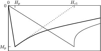
Note that for small inductions $B\ll H_{c1}$ , the diamagnetic response (23) is very different from the usual bulk Abrikosov magnetization (see, e.g., Ref. [24]). The linear decrease in Eq. (23) extrapolates to $M=0$ at $H=H_{c1}$ . The full solution of Eq. (3) for the permeability (21) leads to the magnetic response illustrated in Fig. 4.

II.2 Rectangular strips - Formalism

Having familiarized ourselves with the results for the elliptic strip, we turn our attention to strips with rectangular shape, i.e., samples with constant thickness $d$ as opposed to the ellipse where the height is changing over the entire sample width. Specifically, we will consider (smooth) sample edges with a typical radius of curvature $\gtrsim d$ in contrast to the much sharper edge of the ellipse where the radius of curvature is $d^{2}/4w\ll d$ . We consider a set of coplanar (in the $xy$ -plane) and parallel superconducting strips of infinite length (along $y$ ), each with a rectangular shape of width $2w$ (along $x$ ) and thickness $d\ll 2w$ (along $z$ ), subject to a perpendicular magnetic field $H$ along $z$ . The strip thickness $d$ is assumed to be the smallest geometric length and is set to zero in the following mathematical analysis; its finite value is properly reinstalled through appropriate boundary conditions. Because the system is effectively two-dimensional, we express the magnetic field $\boldsymbol{B}(x,z)$ in the $xz$ -plane through the complex function[4] $\mathcal{B}(\xi)=B_{z}(x,z)+iB_{x}(x,z)$ , with the two-dimensional coordinate $(x,z)$ replaced by the complex variable $\xi=x+iz$ . The magnetostatic problem of solving the Laplace equation ( $\Delta\boldsymbol{B}=0$ ) for $\boldsymbol{B}$ is translated to a problem in complex analysis, where the holomorphic function $\mathcal{B}(\xi)$ satisfies the Cauchy-Riemann equations (correspnding to the magnetostatic equations $\nabla\cdot\boldsymbol{B}=0$ and $\nabla\wedge\boldsymbol{B}=0$ ) in the superconductor-free region; the presence of the superconductor is accounted for through appropriate boundary conditions. The latter derive from two physical conditions: on the one hand, no vortices are present in regions where current is flowing, i.e.,

	$\displaystyle B_{z}(x)$	$\displaystyle=0\quad\mathrm{when}\quad I(x)\neq 0.$	(24)
Here and below we simply call ‘current’ the sheet current density $I(x)$ flowing between $z_{\pm}=\pm d/2$ . On the other hand, no currents flow in the vortex-filled regions,
	$\displaystyle I(x)$	$\displaystyle=0\quad\mathrm{when}\quad B_{z}(x)\neq 0.$	(25)

This last condition neglects the microscopic structure of the vortex state by treating the penetrated region as magnetically inactive, $\mu=1$ ; the accuracy of this simplification will be discussed later in this section. Using Ampère’s law

\displaystyle I(x)=\frac{c}{2\pi}B_{x}(x,0^{+})=\frac{c}{2\pi}\mathrm{Im}[\mathcal{B}(x+i0^{+})],

(26)

the boundary conditions (24) and (25) transform to

	$\displaystyle B_{z}(x)$	$\displaystyle=0\quad\mathrm{when}\quad B_{x}(x)\neq 0,\ \mathrm{and}$		(27)
	$\displaystyle B_{x}(x)$	$\displaystyle=0\quad\mathrm{when}\quad B_{z}(x)\neq 0.$		(28)

For a single strip centered a the origin ( $\xi=0$ ) the holomorphic field

\displaystyle\mathcal{B}(\xi)

\displaystyle=H\sqrt{\frac{\xi^{2}-b_{0}^{2}(H)}{\xi^{2}-w^{2}}}

(29)

is known to satisfy all the above requirements[4]; the parameter $b_{0}$ then determines the field configuration of the entire system. For the double strip studied below, the corresponding expression reads

\displaystyle\mathcal{B}(\xi)

\displaystyle=H\sqrt{\frac{[\xi^{2}-b_{1}^{2}(H)][\xi^{2}-b_{2}^{2}(H)]}{(\xi^{2}-s^{2})(\xi^{2}-W^{2})}}.

(30)

Here, the strips are arranged symmetrically, extending between $\pm s$ and $\pm W$ (with $W=s+2w$ ) on the $x$ -axis.

In order to specify the field and current distributions for these geometries, the parameters $b_{0}$ , $b_{1}$ , and $b_{2}$ (with $0\leq b_{0}<w$ and $s<b_{1}\leq b_{2}<W$ ) describing the boundaries of the field-filled region have to be determined from two physical conditions: First, the net current along each strip vanishes, i.e.,

\displaystyle\int_{\mathrm{strip}}\!\!\!\!\!dx\,I(x)

\displaystyle=0.

(31)

This (first) condition is independent of the magnetic state of the strips, Meissner or Shubnikov. The second condition regulates the penetration process of vortices into the superconducting sample. In the Meissner phase, no field penetrates the superconductor and the width of the vortex dome vanishes, imposing the (second) condition

\displaystyle\left.\begin{aligned} b_{0}&=0&&\textrm{for the single, or}\\ b_{1}&=b_{2}&&\textrm{for the double}\end{aligned}\right.

(32)

strip geometry. The second condition for the penetrated state derives from the analysis of vortex penetration at the sample edge. We consider a smooth edge of shape $z_{\pm}(r)=\pm\ell(r)/2$ with $r$ measured from the sample edge, rising to $\ell=d$ within a distance $r\approx d/2$ (e.g., $\ell(r<d/2)=\sqrt{2rd}$ ). The (tangential) field $H_{\mathrm{edge}}$ at the surface is assumed constant and generates a current density $j=cH_{\mathrm{edge}}/4\pi\lambda$ at the sample boundary, with $\lambda$ denoting the London penetration depth, $\lambda\ll d$ . A simple geometrical consideration provides us with the sheet current $I(r)=2(cH_{\mathrm{edge}}/4\pi)\sqrt{1+[\ell^{\prime}(r)/2]^{2}}$ and using Eq. (13), we obtain the rise of the vortex energy near the edge

\displaystyle U_{\mathrm{geo}}(r)

\displaystyle=\varepsilon_{l}\ell(r)-\frac{\Phi_{0}H_{\mathrm{edge}}}{2\pi}\int\limits_{0}^{r}du\,\sqrt{1+[\ell^{\prime}(u)/2]^{2}}.

(33)

For a smooth edge with radius of curvature $\gtrsim d$ we have $\ell^{\prime}\gg 1$ for $r\ll d$ (consistent with a roughly constant field $H_{\mathrm{edge}}$ ) and we can simplify the above expression to read

\displaystyle U_{\mathrm{geo}}(r)

\displaystyle=\varepsilon_{l}\ell(r)\Big[1-\frac{\Phi_{0}H_{\mathrm{edge}}}{4\pi\varepsilon_{l}}\Big].

(34)

Hence, we find that the energy barrier for vortex entry is eliminated when the local field strength reaches the first critical field $H_{\mathrm{edge}}=H_{c1}=4\pi\varepsilon_{l}/\Phi_{0}$ . Once the edge region of width $d$ has been overcome, the vortices are driven to the sample center where they arrange within the vortex dome. The vortices deep inside the sample reduce the field at the edge and the penetration of flux is stopped when $H_{\mathrm{edge}}$ drops below $H_{c1}$ . With a further increase of the external field, vortices continue to penetrate the sample when the condition $H_{\mathrm{edge}}=H_{c1}$ is satisfied again. This stop and go criterion for vortex penetration then is the second condition imposed on the fields in Eqs. (29) and (30) and determines, together with Eq. (31), the parameters $b_{0}$ , $b_{1}$ , and $b_{2}$ .

The above discussion ignores the possible presence of a surface barrier[9] appearing on small length scales below $\lambda$ . In the most effective case, this barrier further retards the penetration of vortices until the local field reaches the critical strength $H_{\mathrm{edge}}\sim H_{c}$ . In order to deal with the general situation accounting for effects due to a surface barrier we denote the local critical field for vortex penetration by $H_{s}$ ( $H_{c1}<H_{s}<H_{c}$ ). The second condition determining the fields Eqs. (29) and (30) in the penetrated ( $H>H_{p}$ ) state then can be cast in the form

\displaystyle H_{\mathrm{edge}}

\displaystyle=H_{s}.

(35)

The above equation replaces the condition Eq. (32) valid for the Meissner phase. In the regime of very high fields, $H>H_{s}$ , diamagnetic screening becomes small and the field strength at the sample edge lines up with the applied field, $H_{\mathrm{edge}}\approx H$ ; however, this large-field limit will not be considered below.

Finally, we comment on the precision of this second condition: The field strengths in Eqs. (29) and (30) show square-root singularities near the sample edges. The description of the spacial dependence of the field when approaching the edges to distances smaller than $d$ then requires a detailed analysis of the edge region. On the other hand, the typical scale for the field strength needed for overcoming the edge region can be obtained by the considerations presented above, once we have a proper definition for the edge field $H_{\mathrm{edge}}$ at our disposal. Below, we identify this field strength with the field evaluated a distance $d/2$ away from the edge, $H_{\mathrm{edge}}=B_{z}(r=-d/2)$ .

The surface barrier retarding the penetration of flux appears on the small length scale between $\lambda$ (at low fields of order $H_{c1}$ ) and $\xi$ (near $H_{c}$ ). On the contrary, the geometric energy barrier is a macroscopic object appearing on the scale $d$ . We define the geometric barrier $U_{b}$ of a platelet sample as the maximum of Eq. (33) that is reached near $d$ . The second term in Eq. (33) then reduces the geometric barrier linearly to zero at $H_{\mathrm{edge}}=H_{c1}$ and the barrier takes the functional form

\displaystyle U_{b}=\varepsilon_{l}d\Big(1-\frac{H_{\mathrm{edge}}}{H_{c1}}\Big)=\varepsilon_{l}d\Big(1-\frac{H}{H_{p}}\frac{H_{s}}{H_{c1}}\Big)

(36)

where the first (second) equality expresses the barrier in terms of the local (asymptotic) field (note that field penetration only starts when $H_{\mathrm{edge}}=H_{s}$ , where the additional surface barrier has disappeared). While the geometric barrier (36) only vanishes when the local field reaches $H_{c1}$ , the vortex state may become thermodynamically stable at a lower equilibrium field $H_{\mathrm{eq}}$ , defined as the applied field where a global minimum of the energy profile Eq. (13) develops inside the sample. For the single (double) strip, this minimum appears at $x_{0}=0$ ( $x_{0}=b$ ) and $H_{\mathrm{eq}}$ is determined from the condition

\displaystyle\varepsilon_{l}d-\frac{\Phi_{0}}{c}\int\limits_{e}^{x_{0}}du\,I(u)\Bigg|_{H=H_{\mathrm{eq}}}\!\!\!\!=0,

(37)

where $e$ denotes the position of the sample edge penetrated first, $e=w$ for the single strip and $e=s$ for the double strip, see Sec. II.4. The geometrical barrier at the thermodynamic field $H_{\mathrm{eq}}$

\displaystyle U_{b}^{\mathrm{eq}}=\varepsilon_{l}d\Big(1-\frac{H_{\mathrm{eq}}}{H_{p}}\frac{H_{s}}{H_{c1}}\Big)

(38)

then provides us with a measure for the irreversibility of the system, see Fig. 3.

Having analyzed and determined the conditions determining the parameters $b_{0}$ , $b_{1}$ , and $b_{2}$ in the expressions (29) and (30) for the magnetic field, we now are in a position to evaluate the magnetic response (magnetization) of the sample. For this purpose, we make use of Ampère’s law and write the holomorphic field in the form (Biot-Savart, see also Ref. [21])

\displaystyle\mathcal{B}(\xi)

\displaystyle=H-\frac{2}{c}\int_{\text{strips}}\!\!\!\!du\,\frac{I(u)}{\xi-u}.

(39)

This field assumes the asymptotic form (we expand for $|\xi|\gg w$ )

\displaystyle\mathcal{B}(\xi)

\displaystyle=H-\frac{2}{c\,\xi^{2}}\int_{\text{strips}}\!\!\!\!\!\!du\,u\,I(u)+\mathcal{O}(\xi^{-4}),

(40)

where we have used that the total current in each strip vanishes. The second term in Eq. (40) describes the field of a line of magnetic dipoles distributed along the $y$ -axis ( $\xi=0$ ). We thus identify the magnetization $M$ per unit length (from here on called magnetization) with the expression

\displaystyle M

\displaystyle=\frac{1}{c}\int_{\mathrm{strips}}\!\!\!\!du\,u\,I(u).

(41)

This result differs from the usual textbook formula[25, 11]

\displaystyle\mathcal{M}=\frac{1}{2c}\int d^{3}r\;\boldsymbol{r}\times\boldsymbol{j}(\boldsymbol{r})

(42)

relating the total magnetic moment $\mathcal{M}$ to its generating current density $\boldsymbol{j}(\boldsymbol{r})$ flowing in a loop. The translation invariant 2D result (41) can easily be shown to be consistent with the 3D textbook formula for a finite size ( $2L$ along $y$ ) strip taking also into account the currents $j_{x}(y)$ flowing near the ends $y=\pm L$ of the strips and closing the loop.

Formally expanding the left-hand side of Eq. (40) in $\xi^{-2}$ and comparing terms, the magnetization can be rewritten as

\displaystyle M(H)

\displaystyle=-\frac{1}{2}\left.\frac{\partial\mathcal{B}(\xi)}{\partial(1/\xi^{2})}\right|_{\xi^{-2}\to 0}\!.

(43)

The magnetic responses of the single and double strip geometries [as obtained from Eqs. (43), (29), and (30)] take the particularly simple form

	$\displaystyle M(H)$	$\displaystyle=-\frac{H}{4}(w^{2}-b_{0}^{2}),$		(44)
	$\displaystyle M(H)$	$\displaystyle=-\frac{H}{4}(W^{2}+s^{2}-b_{1}^{2}-b_{2}^{2}).$		(45)

II.3 Single strip

We briefly review the physics of geometrical barriers for a single strip derived by Zeldov and co-workers[4]. The function $\mathcal{B}(\xi)$ , holomorphic in the superconductor-free region and satisfying the required boundary conditions, is given by Eq. (29). On the $x$ -axis ( $z=0$ ), the magnetic field component along $z$ is given by

\displaystyle B_{z}(x)

\displaystyle=\left\{\begin{aligned} &H\sqrt{\frac{b_{0}^{2}-x^{2}}{w^{2}-x^{2}}}&&\mathrm{for\ }|x|\leq b_{0},\\ &H\sqrt{\frac{x^{2}-b_{0}^{2}}{x^{2}-w^{2}}}&&\mathrm{for\ }w\leq|x|,\\ &0&&\mathrm{for\ }b_{0}\leq|x|\leq w.\end{aligned}\right.

(46)

The region $|x|\leq b_{0}$ describes the field-penetrated part of the sample where $B_{z}$ is finite. The current $I(x)$ flows in the complementary regions $b_{0}\leq|x|\leq w$ inside the strip; making use of Eq. (29) and Ampere’s law in the form of Eq. (26) we obtain the current

\displaystyle I(x)

\displaystyle=-\frac{Hc}{2\pi}\frac{x}{|x|}\sqrt{\frac{x^{2}-b_{0}^{2}}{w^{2}-x^{2}}}.

(47)

The anti-symmetry of $I(x)$ guarantees the vanishing of the total current as required by Eq. (31). The diamagnetic response resulting from these currents can be obtained with the formula given in Eq. (41) or directly via Eq. (44).

II.3.1 Meissner state

In the Meissner state the field is fully expelled from the strip, $b_{0}=0$ , and Eqs. (46) and (47) simplify to

\displaystyle B_{z}(x)

\displaystyle=\left\{\begin{aligned} &H\frac{x}{\sqrt{x^{2}-w^{2}}}&&\mathrm{for\ }w\leq|x|,\\ &0&&\mathrm{for\ }|x|\leq w.,\end{aligned}\right.

(48)

and

\displaystyle I(x)

\displaystyle=-\frac{Hc}{2\pi}\frac{x}{\sqrt{w^{2}-x^{2}}},

(49)

respectively. This anti-symmetric current density preserves the Meissner state and is identical to the one for the elliptic strip discussed before, see Eq. (11). The divergencies in Eq. (48) at $x=\pm w$ have to be cut at the distance $\sim d$ away from the edges and we choose the specific value $d/2$ . The local field strength at the edge (we drop corrections of higher order in $d/w$ )

\displaystyle H_{\mathrm{edge}}

\displaystyle\equiv B_{z}(w+d/2)\simeq H\sqrt{\frac{w}{d}}

(50)

then is enhanced by the factor $\sqrt{w/d}$ . This enhancement is parametrically smaller as compared to the flat ellipsoid with corresponding dimensions where the enhancement factor is $2w/d$ . The response of the superconducting strip in the Meissner state produces the magnetization [see Eq. (44) with $b_{0}=0$ ]

\displaystyle M(H)

\displaystyle=-\frac{H}{4}w^{2},

(51)

corresponding to the expulsion of the field $H$ from a region of size $\sim w^{2}$ . Similar to the currents, the diamagnetic response is identical with that of an elliptic sample, see Eq. (12).

The Meissner state becomes unstable at $H=H_{p}$ as determined by the condition Eq. (35); with the field enhancement given in Eq. (50), we find

\displaystyle H_{p}

\displaystyle\simeq H_{s}\sqrt{\frac{d}{w}}

(52)

and the (maximum) magnetization at penetration reads

\displaystyle M_{p}

\displaystyle=-\frac{H_{s}}{4}w^{2}\sqrt{\frac{d}{w}}=-\frac{H_{p}}{4}w^{2}.

(53)

As discussed above, the precise value for $H_{p}$ depends on the details of the edge geometry; the latter will modify the result (52) by a numerical factor of order unity and affect all further results in this section in a straightforward way. For an elliptic strip, the larger field enhancement near the edges causes the penetration field Eq. (15) to be parametrically ( $\sim\!\!\sqrt{d/w}$ ) smaller than that of the platelet sample.

Although penetration is delayed to $H_{p}$ , a field-filled state is thermodynamically stable (yet inaccessible due to the geometric barrier) beyond the equilibrium field

\displaystyle H_{\mathrm{eq}}=H_{c1}\frac{d}{2w}

(54)

as obtained from evaluating Eq. (37). The geometric barrier height [from Eq. (38) with $H_{s}=H_{c1}$ ] at that specific field amounts to

\displaystyle U_{b}^{\mathrm{eq}}=\varepsilon_{l}d\,\big(1-\sqrt{d/4w}\big).

(55)

II.3.2 Penetrated state

Increasing the external field $H$ beyond $H_{p}$ , vortices accumulate inside the strip in a dome-like density distribution of width $2b_{0}$ . The field (current) profile along the $x$ -axis ( $z=0$ ) is given by the general form (46) [(47)]. The absence of a net current inside the strip is satisfied by symmetry, $I(-x)=-I(x)$ . The evolution

\displaystyle b_{0}^{2}(H)

\displaystyle\simeq w^{2}[1-(H_{p}/H)^{2}]

(56)

of the dome width as a function of the applied field $H$ is determined by imposing a critical field strength at the edges, i.e., by solving Eq. (35) for $H_{\mathrm{edge}}=B_{z}(w+d/2)$ . The induction in the vortex dome takes the maximal value $(b_{0}/w)H$ at the gap center. For a largely penetrated strip, $w-b_{0}\ll w$ , the induction is almost uniform and equal to the external field, $B(x)\approx H$ . The presence of vortices inside the superconductor reduces the diamagnetic response, see Eq. (44)

\displaystyle M(H)

\displaystyle\simeq-\frac{H_{p}^{2}}{4H}w^{2}=-\frac{H_{s}^{2}}{4H}wd.

(57)

The applicability of the expressions (56) and (57) is limited to the regime where the screening currents flow in regions much wider than the sample thickness ( $w-b_{0}\gg d$ ), a limit reached when the external field $H$ is very large, of order $H_{s}$ . At this point, the strip is almost uniformly penetrated by the field with $B_{z}\approx H_{s}$ , while the remaining screening currents flow in a narrow region of width $\sim d$ near the edges, maintaining a diamagnetic response

\displaystyle M(H_{s})

\displaystyle\approx-\frac{H_{p}}{4}w^{2}\sqrt{\frac{d}{w}}.

(58)

Predictions on the system’s behavior for very large applied fields $H>H_{s}$ require a precise knowledge of the field distribution near the sample edge, a topic which is beyond our present analysis.

The penetration process of vortices across a geometric energy barrier in a platelet strip features a hysteretic behavior[4, 26]; upon reduction of the external field from a maximal value $H^{\star}$ , the flux $\phi_{d}^{\star}=\phi_{d}(H^{\star})$ of vortices through the sample, where

\displaystyle\phi_{d}=\int\limits_{-b_{0}}^{b_{0}}dx\,B_{z}(x),

(59)

is trapped unless the vortex dome boundaries reach the sample edges. Evaluating the above flux with the field (46), we find

\displaystyle\phi_{d}=2wH\Big[\E(b_{0}/w)-\frac{w^{2}-b_{0}^{2}}{w^{2}}\K(b_{0}/w)\Big],

(60)

with $\K$ ( $\E$ ) the complete elliptic integral of the first (second) kind defined according to standard textbooks on mathematical functions; e.g., see Eqs. (17.2.18)-(17.3.3) of Ref. [27],

	$\displaystyle\K(\kappa)$	$\displaystyle=\int_{0}^{\pi/2}\frac{d\theta}{\sqrt{1-\kappa^{2}\sin\!{}^{2}(\theta)}},$		(61)
	$\displaystyle\E(\kappa)$	$\displaystyle=\int_{0}^{\pi/2}d\theta\sqrt{1-\kappa^{2}\sin\!{}^{2}(\theta)}.$		(62)

For $\kappa\ll 1$ , the elliptic functions show the limiting behavior

	$\displaystyle\K(\kappa)$	$\displaystyle=\frac{\pi}{2}\Big[1+\frac{\kappa^{2}}{4}+\frac{9\kappa^{4}}{64}+\mathcal{O}(\kappa^{6})\Big],$		(63)
	$\displaystyle\E(\kappa)$	$\displaystyle=\frac{\pi}{2}\Big[1-\frac{\kappa^{2}}{4}-\frac{3\kappa^{4}}{64}+\mathcal{O}(\kappa^{6})\Big],$		(64)

while for the opposite limit, $\kappa=\sqrt{1-\nu}$ with $\nu\ll 1$ , we find

	$\displaystyle\K(\sqrt{1-\nu})$	$\displaystyle=\frac{1}{2}\log\Big(\frac{16}{\nu}\Big)-\frac{\nu}{8}\Big[2-\log\Big(\frac{16}{\nu}\Big)\Big]+\mathcal{O}(\nu^{2}),$		(65)
	$\displaystyle\E(\sqrt{1-\nu})$	$\displaystyle=1-\frac{\nu}{4}\Big[1-\log\Big(\frac{16}{\nu}\Big)\Big]+\mathcal{O}(\nu^{2}).$		(66)

The constraint $\phi_{d}(H<H^{\star})=\phi_{d}^{\star}$ reduces to a condition for the dome width $b_{0}(H)$ of the form

\displaystyle\E(b_{0}/w)-\frac{w^{2}-b_{0}^{2}}{w^{2}}\K(b_{0}/w)

\displaystyle=\frac{\phi_{d}^{\star}}{2w\,H},

(67)

in agreement with Ref. [5]. The left-hand side is limited by unity from above (for $b_{0}=w$ ). Upon decreasing $H$ , the vortex dome expands over the sample until reaching the edge. Since for a large dome, $w-b_{0}\ll w$ , the induction is uniform and equal to $H$ , we find that vortices leave the sample at $H=H_{\mathrm{ex}}=\phi_{d}^{\star}/2w$ where formally $b_{0}=w$ and $M=0$ .

For a narrow dome $b_{0}/w\ll 1$ , the above condition (67) can be simplified using the asymptotic expressions (63) and (64) for the elliptic functions; to lowest (quadratic) order in $\kappa=b_{0}/w$ , we find

\displaystyle\frac{b_{0}^{2}}{w^{2}}

\displaystyle=\frac{4}{\pi}\frac{H_{\mathrm{ex}}}{H}.

(68)

The growth of the dome width $b_{0}^{2}=b_{0}^{\star}{}^{2}H^{\star}/H$ [with $b_{0}^{\star}=b_{0}(H^{\star})$ ] results in a magnetic response of the form

\displaystyle M(H)

\displaystyle=-\frac{H}{4}w^{2}+\frac{H^{\star}}{4}{b_{0}^{\star}}^{2}

(69)

with a slope identical to the Meissner state. Higher order corrections (quartic in $\kappa=b_{0}/w$ ) are straight forwardly obtained from Eqs. (63) and (64): the condition (67) then yields

\displaystyle\frac{b_{0}^{2}}{w^{2}}

\displaystyle=4\bigg\{\sqrt{1+\frac{H^{\star}}{H}\Big[\Big(1+\frac{1}{4}\frac{b_{0}^{\star}{}^{2}}{w^{2}}\Big)^{2}-1\Big]}-1\bigg\}.

(70)

Inserting this solution into the expression (44) for the magnetization, the Meissner slope is corrected according to

	$\displaystyle\frac{dM}{dH}$	$\displaystyle=-\frac{w^{2}}{4}\bigg\{1-\frac{1}{2}\Big(\frac{H^{\star}}{H}\Big)^{2}\Big[\Big(1+\frac{1}{4}\frac{b_{0}^{\star}{}^{2}}{w^{2}}\Big)^{2}-1\Big]^{2}\bigg\}$
		$\displaystyle\approx-\frac{w^{2}}{4}\Big[1-\frac{1}{8}\Big(\frac{H^{\star}}{H}\frac{b_{0}^{\star}{}^{2}}{w^{2}}\Big)^{2}\Big].$		(71)

The rapid growth of the dome-width on both the field-increasing (filling the dome with additional flux) and decreasing (expanding the dome at fixed flux) branches leads to a fast violation of the condition $b_{0}\ll w$ assumed above and hence these results have a rather limited range of validity. Another limit is reached when $b_{0}$ is large, $w-b_{0}\ll w$ . Defining $\nu=1-b_{0}^{2}/w^{2}$ , the asymptotic expressions (65) and (66) can be used to simplify (up to linear order in $\nu$ ) the condition (67) to

\displaystyle 1-\frac{\nu}{4}\Big[\log\Big(\frac{16}{\nu}\Big)+1\Big]

\displaystyle=\frac{H_{\mathrm{ex}}}{H}.

(72)

In most of the $M$ - $H$ -diagram, the system’s magnetic response on the descending branch then is given by $M(H)=-Hw^{2}\nu(H)/4$ . Taking the derivative of $M$ with respect to $H$ , the slope of the descending branch can be evaluated and, after some reordering, we find that

\displaystyle\frac{dM}{dH}

\displaystyle=-\frac{w^{2}}{4}\frac{4-\nu}{\log(16/\nu)}.

(73)

The derivative (73) deviates from the Meissner slope $-w^{2}/4$ by a numerical factor which assumes the value $\approx 1.01$ for $\nu\sim 1/2$ , when the previous approach of a narrow dome predicts a perfect Meissner slope [see Eq. (69)]. In the regime of applicability, where $\nu$ may change by several orders of magnitude, the factor $(4-\nu)/\log(16/\nu)$ changes noticeably but not parametrically. Typically, the slope of the descending branch is numerically close to the Meissner slope within the parameter range under consideration, see Fig. 5. For large reversal fields $H^{\star}\gg H_{p}$ , we replace the parameter $\nu(H)$ by its value at the field reversal $\nu(H^{\star})=\nu^{\star}=1-b_{0}^{\star}{}^{2}/w^{2}=(H_{p}/H^{\star})^{2}$ , where we have used Eq. (56). The magnetization

\displaystyle M(H)=M(H^{\star})-\frac{H-H^{\star}}{4}w^{2}\frac{4-\nu^{\star}}{\log(16/\nu^{\star})}

(74)

as obtained from Eq. (73) and integration from $H^{\star}$ to $H$ provides a good description of the descending branch in this regime, see Fig. 5.

As the boundaries of the dome approach the edges of the strip to a distance $\sim d$ (which is the case when $H\approx[1+\mathcal{O}(d/w)]H_{\mathrm{ex}}$ ) the precise geometric shape of the sample edge needs to be taken into account, requiring a more accurate analysis going beyond the present description. An attempt to cope with this situation has been undertaken by Zeldov and co-workers in Refs. [26, 28, 29].

II.3.3 Magnetization of the vortex dome

The physical properties of quantized flux lines appeared in the above analysis merely as a criterion for vortex entry at the sample edges. The vortex dome in the penetrated state has been described by a smooth field $B_{z}(x)\neq 0$ residing in a magnetically inactive medium with $\mu=1$ whose extend $[-b_{0},b_{0}]$ derives from the solution ${\cal B}(\xi)$ of the boundary value problem. In reality, the vortex state in the dome is described by a field $h(x)$ modulated on the scale of the inter-vortex distance due to vortex currents. In the following, we show that the currents associated with the vortex state in the dome generate a magnetization which remains small as compared to the magnetization produced by the screening currents flowing in the field-free regions.

An analogous problem appears in the context of surface barriers as discussed by Clem[9] and by Koshelev[30]: quite similar to our analysis, in Ref. [9] the vortex-penetrated bulk, separated from the boundary by a layer of screening (Meissner) currents, has been described by an induction $B_{z}$ averaged over the inter-vortex spacing. This approximation neglects all field and current modulations due to the vortex state and the resulting magnetization density is given by[9]

\displaystyle m(H)

\displaystyle=-\frac{H}{4\pi}\big[1-\sqrt{1-(H_{s}/H)^{2}}\,\big].

(75)

A way to account for the local currents in the vortex state has been proposed by Koshelev[30], who found that these contribute a paramagnetic correction $\delta m=(\sqrt{3}/48)(\Phi_{0}/4\pi\lambda^{2})$ to the magnetization density $m(H)$ in the limit $B\gg\Phi_{0}/\lambda^{2}$ . Following a similar ideology as in Ref. [30], we describe the flux-filled region in terms of a vortex lattice along $z$ with vortex rows aligned along $y$ and separated by $b_{\scriptscriptstyle{\triangle}}$ in the $x$ -direction with $b_{\scriptscriptstyle{\triangle}}^{2}=(3/4)^{1/2}\Phi_{0}/B_{z}$ . While in Ref. [30] $B_{z}(x)$ was determined self-consistently, here, we estimate the corrections to the magnetization by adopting the averaged field $B_{z}(x)$ obtained from the above analytic solution. In our strip geometry, the spacing $b_{\scriptscriptstyle{\triangle}}$ between vortex-rows slowly varies along $x$ , as the induction $B_{z}$ changes on macroscopic length scales. The connection between the local field $h(x)$ and the induction $B_{z}(x)$ is given by the average

\displaystyle B_{z}(x)=\frac{1}{b_{\scriptscriptstyle{\triangle}}}\int\limits_{x-b_{\scriptscriptstyle{\triangle}}/2}^{x+b_{\scriptscriptstyle{\triangle}}/2}dx^{\prime}h(x^{\prime}).

(76)

The local field $h(x)$ satisfies the one-dimensional London equation $\lambda^{2}h^{\prime\prime}(x)+h(x)=0$ between the vortex rows with the boundary conditions replaced by the constraint (76). For a slowly varying dome profile, i.e., $b_{\scriptscriptstyle{\triangle}}\partial_{x}B_{z}(x)\ll B_{z}(x)$ , we obtain the field modulation between vortex rows

\displaystyle h(x)

\displaystyle\approx B_{z}(x_{c})\frac{b_{\scriptscriptstyle{\triangle}}}{2\lambda}\frac{\cosh[(x-x_{c})/\lambda]}{\sinh(b_{\scriptscriptstyle{\triangle}}/2\lambda)},

(77)

with $x_{c}$ the center between the two adjacent rows and $|x-x_{c}|<b_{\scriptscriptstyle{\triangle}}/2$ . Ampère’s law then provides us with the current profile

\displaystyle j(x)

\displaystyle\approx-\frac{B_{z}(x_{c})c}{4\pi}\frac{b_{\scriptscriptstyle{\triangle}}}{2\lambda^{2}}\frac{\sinh[(x-x_{c})/\lambda]}{\sinh(b_{\scriptscriptstyle{\triangle}}/2\lambda)}

(78)

and we can evaluate the associated average magnetization density at the vortex location $x_{v}$

	$\displaystyle m(x_{v})$	$\displaystyle\approx\frac{1}{b_{\scriptscriptstyle{\triangle}}c}\int\limits_{x_{v}-b_{\scriptscriptstyle{\triangle}}/2}^{x_{v}+b_{\scriptscriptstyle{\triangle}}/2}dx^{\prime}x^{\prime}j(x^{\prime})$		(79)
		$\displaystyle\approx\frac{B_{z}(x_{v})}{4\pi}\Big[1-\frac{b_{\scriptscriptstyle{\triangle}}}{2\lambda}\frac{1}{\sinh(b_{\scriptscriptstyle{\triangle}}/2\lambda)}\Big].$		(80)

For small fields $B_{z}\ll H_{c1}$ , we find that $m(x)\approx B_{z}(x)/4\pi$ , while the magnetization density saturates at $(\Phi_{0}/4\pi\lambda^{2})\sqrt{3}/48$ for large fields $B_{z}\gg H_{c1}$ , consistent with the results presented in Ref. [30]. In order to estimate the correction to the strips’ magnetic response, we introduce the upper bound

\displaystyle m(x)\leq\frac{B_{z}(x)}{4\pi}\frac{H_{c1}}{H_{c1}+B_{z}(x)}

(81)

with the correct asymptotic behavior for $B\ll H_{c1}$ and logarithmically [ $\propto\log(\lambda/\xi)$ ] overestimating the magnetization when $B\gg H_{c1}$ . Integrating $m(x)$ over the dome and replacing the dome profile $B_{z}(x)$ by its maximum $Hb_{0}/w$ at the center, see Eq. (46), we obtain the bound

\displaystyle\delta M<\frac{H}{4\pi}\frac{H_{c1}}{H_{c1}+Hb_{0}/w}\frac{b_{0}^{2}}{w^{2}}2wd.

(82)

For a small dome, $b_{0}\ll w$ , this expression simplifies to

\displaystyle\delta M<\frac{H}{4\pi}\Big(1-\frac{H_{p}^{2}}{H^{2}}\Big)2wd,

(83)

whereas for a large part of the penetrated region $d\ll w-b_{0}(H)\ll w$ , we find that

\displaystyle\delta M<\frac{H}{4\pi}\frac{H_{c1}}{H_{c1}+H}2wd.

(84)

As a result, the correction $\delta M$ due to the reversible magnetization measured on the magnetization $M$ of the screening currents Eq. (57) is bounded from above by

\displaystyle\frac{\delta M}{M}

\displaystyle<\frac{2}{\pi}\frac{H^{2}}{H_{s}^{2}}\frac{H_{c1}}{H_{c1}+H}.

(85)

In the absence of a surface barrier ( $H_{s}=H_{c1}$ ) these corrections are small and become of order unity at the largest fields $H\sim H_{c1}$ where our analysis applies. In the presence of a large surface barrier where $H_{s}\gg H_{c1}$ , the corrections are even smaller and reach a maximum $\sim H_{c1}/H_{s}\ll 1$ when $H\sim H_{s}$ . We conclude that the corrections arising from the vortex currents can be omitted in the single strip geometry.

II.4 Double strip

We now investigate the double-strip configuration defined in Fig. 1, a system of two coplanar, parallel strips of width $2w$ each and separated by a gap $2s$ . Assuming a gap that is large as compared to the strip thickness, $s\gg d$ , the system can be treated within the framework introduced in Sec. II.2. The holomorphic function has been presented in Eq. (30), from which the [symmetric, $B_{z}(-x)=B_{z}(x)$ ] field and [anti-symmetric, $I(-x)=-I(x)$ ] current distribution on the $x$ -axis can be readily deduced

\displaystyle\frac{B_{z}(x)}{H}

\displaystyle=\left\{\begin{aligned} &\sqrt{\frac{(b_{1}^{2}-x^{2})(b_{2}^{2}-x^{2})}{(s^{2}-x^{2})(W^{2}-x^{2})}}&&\mathrm{for\ }0\leq x\leq s,\\ &\sqrt{\frac{(x^{2}-b_{1}^{2})(b_{2}^{2}-x^{2})}{(x^{2}-s^{2})(W^{2}-x^{2})}}&&\mathrm{for\ }b_{1}\leq x\leq b_{2},\\ &\sqrt{\frac{(x^{2}-b_{1}^{2})(x^{2}-b_{2}^{2})}{(x^{2}-s^{2})(x^{2}-W^{2})}}&&\mathrm{for\ }W\leq x,\\ &0&&\mathrm{otherwise},\end{aligned}\right.

(86)

and

\displaystyle\frac{2\pi I(x)}{cH}

\displaystyle=\left\{\begin{aligned} &\sqrt{\frac{(b_{1}^{2}-x^{2})(b_{2}^{2}-x^{2})}{(x^{2}-s^{2})(W^{2}-x^{2})}}&&\mathrm{for\ }s\leq x\leq b_{1},\\ &-\sqrt{\frac{(x^{2}-b_{1}^{2})(x^{2}-b_{2}^{2})}{(x^{2}-s^{2})(W^{2}-x^{2})}}&&\mathrm{for\ }b_{2}\leq x\leq W,\\ &0&&\mathrm{otherwise}.\end{aligned}\right.

(87)

The resulting magnetization is given by Eq. (45).

II.4.1 Meissner state

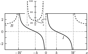
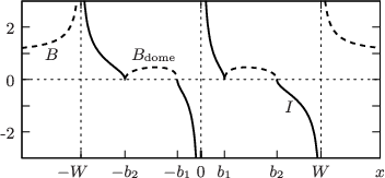
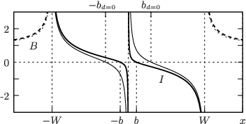
In the (low-field) Meissner state the parameters $b_{1}$ , $b_{2}$ in Eq. (30) coincide, $b_{1}=b_{2}=b$ , with $\pm b$ marking the the positions inside the strips where the current density changes sign (see Fig. 6). The magnetic field component $B_{z}$ [from Eq. (86)] is non-vanishing whenever $|x|\leq s$ or $W\leq|x|$ and reads

\displaystyle B_{z}(x)

\displaystyle=H\frac{|x^{2}-b^{2}|}{\sqrt{(x^{2}-s^{2})(x^{2}-W^{2})}}.

(88)

In the complementary region $s\leq|x|\leq W$ , the screening current

\displaystyle I(x)

\displaystyle=-\frac{Hc}{2\pi}\frac{x}{|x|}\frac{x^{2}-b^{2}}{\sqrt{(x^{2}-s^{2})(W^{2}-x^{2})}}

(89)

guarantees a perfect diamagnetic (Meissner) response

\displaystyle M(H)

\displaystyle=-\frac{H}{4}(W^{2}+s^{2}-2b^{2}),

(90)

with $b$ independent of $H$ . The condition (31) that no net current flows along each strip requires that

\displaystyle\int\limits_{s}^{W}\frac{dx\,x^{2}}{\sqrt{(x^{2}-s^{2})(W^{2}-x^{2})}}

\displaystyle=\int\limits_{s}^{W}\frac{dx\,b^{2}}{\sqrt{(x^{2}-s^{2})(W^{2}-x^{2})}},

(91)

from which we find the value of $b$ ,

\displaystyle b^{2}

\displaystyle=W^{2}\frac{\E(\kappa^{\prime})}{\K(\kappa^{\prime})},

(92)

in agreement with Ref. [20]. Here, $\K$ ( $\E$ ) is the complete elliptic integral of the first (second) kind, as defined in Eq. (61) [(62)], and $\kappa^{\prime}=\sqrt{1-\kappa^{2}}$ is the complementary modulus of $\kappa=s/W$ . For large gaps, the double strip behaves as two independent strips: indeed, for $s/w\to\infty$ , the parameter $b$ approaches the sample center $w+s$ and the magnetization assumes the asymptotic value $M(H)\to-Hw^{2}/2$ , twice that of an isolated strip, see Eq. (51).

Let us then focus on the opposite limit $s\ll W=2w+s$ , where the right hand side of Eq. (91) shows a logarithmic divergence $\propto\log(W/s)$ , while the left hand side is regular; in this limit, the parameter $b$ takes the asymptotic form

\displaystyle b^{2}

\displaystyle=\frac{W^{2}}{\log{(4W/s)}},

(93)

and the position $b$ where the current $I(x)$ changes sign is no longer at the sample center but has shifted towards the inner edge, see Figs. 6, 8 and 15. The magnetization (per unit length) (90) to leading order in $s/W$ reads,

\displaystyle M(H)

\displaystyle=-\frac{H}{4}W^{2}\Big[1-\frac{2}{\log(4W/s)}\Big].

(94)

In the limit $s/W\to 0$ , the Meissner slope approaches that of a single strip with double width, see Eq. (51). We conclude that over the full range of gap widths $s$ (from $s\gg W$ down to $s/W\to 0$ ) the slope in the magnetization of the Meissner state increases only by a factor 2.

For the double strip geometry, the flux (per unit length) $\phi_{g}$ passing through the gap $|x|<s$ is defined as the $z$ -component of the magnetic field (88) integrated over the gap width,

\displaystyle\phi_{g}

\displaystyle=\!\!\int\limits_{-s}^{s}\!dx\,B_{z}(x)=2W\Big[\E(\kappa)-\Big(1-\frac{b^{2}}{W^{2}}\Big)\K(\kappa)\Big]H,

(95)

where the elliptic functions are evaluated at $\kappa=s/W$ . In the regime of almost independent strips, $s\gg W$ , the flux $2sH$ of the homogeneous field in the empty gap region is enhanced by half of the flux $\phi_{b}=4wH$ blocked by the two strips, thus adding up to $\phi_{g}\approx(2s+2w)H$ . In the opposite limit $s\ll W$ , the expression (95) for the flux in the gap simplifies to

\displaystyle\phi_{g}

\displaystyle\simeq\frac{\pi b^{2}}{W}H\simeq\frac{\pi W}{\log(4W/s)}H.

(96)

An essential part (up to a logarithmic factor) of the blocked flux $\phi_{b}=2WH$ is pushed through the gap. This slow reduction of $\phi_{g}$ upon reducing $s$ goes hand in hand with an enhancement of the field strength at the gap center

\displaystyle B_{z}(0)

\displaystyle=H\frac{b^{2}}{sW}=\frac{2}{\pi}\frac{\phi_{g}}{2s}=H\frac{W/s}{\log(4W/s)}

(97)

and near the inner edges

\displaystyle B_{z}(s-d/2)

\displaystyle\simeq H\frac{b^{2}}{\sqrt{sd}\,W}=H\frac{W/\sqrt{sd}}{\log(4W/s)}.

(98)

This last expression is parametrically larger than the enhancement observed at the edge of an isolated strip, see Eq. (50). Note that the field inside the gap is far from constant, but increases by a factor $\sqrt{s/d}$ from the gap center to one strip edge, see inset in Fig. 6). On the other hand, the field strength near the outer edges

\displaystyle B_{z}(W+d/2)

\displaystyle\simeq H\frac{W^{2}-b^{2}}{W\sqrt{Wd}}=H\sqrt{\frac{W}{d}}\Big[1-\frac{1}{\log(4W/s)}\Big]

(99)

is comparable to that of an isolated strip, see Eq. (50). From this analysis we conclude that the local critical field $H_{s}$ is first reached near the inner edges, such that the penetration of vortices occurs from inside. The field of first penetration $H_{p}$ then is determined by the condition

\displaystyle H_{\mathrm{edge}}

\displaystyle=B_{z}(s-d/2)=H_{s}

(100)

and making use of Eq. (98) we find that the penetration field for small gaps $s\ll W$

\displaystyle H_{p}

\displaystyle\simeq H_{s}\sqrt{\frac{sd}{W^{2}}}\frac{W^{2}}{b^{2}}=H_{s}\sqrt{\frac{sd}{W^{2}}}\log{(4W/s)}

(101)

is substantially reduced as compared to the one for isolated strips $H_{p}\simeq H_{s}\sqrt{d/w}$ . As discussed for the single strip, see Eq. (52) and thereafter, the precise edge geometry will alter the above expression for $H_{p}$ by a numerical factor of order unity (the same factor as for the single strip), a correction that will be neglected in the following. At penetration $H=H_{p}$ , the Meissner state reaches the maximal diamagnetic response [see Eq. (94)]

\displaystyle M_{p}

\displaystyle=-\frac{H_{s}}{4}W\sqrt{sd}\,\big[\log{(4W/s)}-2\big].

(102)

Upon reducing the gap width $s$ , the penetration field diminishes and the geometrical barrier is more strongly suppressed, see Eq. (36). Vortices become energetically favorable (deep) inside the sample beyond the equilibrium field (we use Eq. (37) in the regime $s\ll W$ )

\displaystyle H_{\mathrm{eq}}=H_{c1}\frac{d}{2W}\Big\{1-\frac{\log[4\log(4W/s)]+1}{2\log(4W/s)}\Big\}^{-1},

(103)

resulting in a geometric barrier (38) at $H_{\mathrm{eq}}$ which decreases with $s$ ,

\displaystyle\frac{U_{b}^{\mathrm{eq}}(s)}{\varepsilon_{l}d}=1-\frac{\sqrt{d/s}}{2\log(4W/s)-\log[4\log(4W/s)]-1}.

(104)

II.4.2 Penetrated state

Increasing the external field beyond its critical value, $H_{p}$ , vortices penetrate the superconductor from the inner edges at $x=\pm s$ and accumulate near the position $b$ inside the strips where the potential $U_{\mathrm{geo}}(x)$ is minimal. The field and currents take the general form given in Eqs. (86) and (87), with the non-trivial vortex state determined by the two boundaries of the vortex dome $b_{1}$ and $b_{2}$ .

These two parameters satisfy the constraint of vanishing net current in each strip

\displaystyle\int_{s}^{b_{1}}dx\,I(x)+\int_{b_{2}}^{W}dx\,I(x)

\displaystyle=0,

(105)

together with the condition [from Eq. (35)]

\displaystyle H_{\mathrm{edge}}=B_{z}(s-d/2)

\displaystyle=H_{s}.

(106)

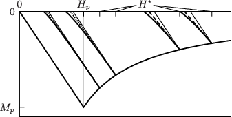
While this constraint locks the field strength at the inner edge to $H_{s}$ , the field strength near the outer edge continuously grows, but remains below $H_{s}$ . In Fig. 7 we show the field and current profiles in the penetrated state for $H=1.2H_{p}$ as obtained from solving Eqs. (105) and (106) numerically. The evolution of the dome’s boundaries and its width $b_{2}-b_{1}$ with increasing field is shown in Fig. 8. The maximal field value in the dome can be estimated with the interpolation formula $B_{\mathrm{dome}}\sim H(b_{2}-b_{1})/W$ .

In order to find analytic results describing the penetrated state, we have to simplify the problem of determining the parameters $b_{1}$ , $b_{2}$ . Evaluating the condition (106) for the field (86) and expressing the result through the penetration field $H_{p}$ , the dome boundaries $b_{1}(H)$ and $b_{2}(H)$ are related via

\displaystyle\frac{\sqrt{b_{1}^{2}-s^{2}}\ b_{2}}{b^{2}}=\frac{H_{p}}{H},

(107)

where $b$ is the (field-independent) zero-current location in the Meissner state, Eq. (92).

It turns out that a perturbative calculation around the penetration field with the small parameter $h=(H-H_{p})/H_{p}\ll 1$ produces results with a very limited range of validity. This is due to the rapid growth of the dome width $b_{2}-b_{1}$ with increasing $h$ , leading to a fast break-down of the approximation. Approaching the problem from the high field limit $H\gg H_{p}$ is more successful: starting from the regime where the dome extends over a large fraction of the strip $b_{1}\ll b_{2}$ , we can adopt another perturbative approach which provides accurate results all the way down to $H_{p}$ . We use the Ansatz $b_{2}=W(1-\nu)^{1/2}$ with $\nu(H)<1$ . For $s\ll b_{1}$ , where Eq. (107) simplifies to

\displaystyle b_{1}=W\frac{b^{2}}{W^{2}}\frac{H_{p}}{H}\frac{1}{\sqrt{1-\nu}},

(108)

the constraint (105) of vanishing net current in the strips can be written as

	$\displaystyle\frac{H_{p}}{H}\frac{b^{2}}{W^{2}}\left[\log{\Big(\frac{4W}{s}\frac{b^{2}}{W^{2}}\frac{H_{p}}{H}\frac{1}{\sqrt{1-\nu}}\Big)}-1\right]$			(109)
	$\displaystyle=\E(\sqrt{\nu})-$	$\displaystyle(1-\nu)\K(\sqrt{\nu}).$

Solving this equation to leading order in $H_{p}/H$ where $\nu\ll 1$ , we find that

\displaystyle\nu(H)

\displaystyle=\frac{4}{\pi}\frac{H_{p}}{H}\frac{b^{2}}{W^{2}}\left[\log{\Big(\frac{4W}{s}\frac{b^{2}}{W^{2}}\frac{H_{p}}{H}\Big)}-1\right].

(110)

To leading order in $\nu(H)$ , the magnetic response in Eq. (45) takes the form $M\simeq-H\nu(H)W^{2}/4$ , resulting in a logarithmic field-dependence

\displaystyle M(H)

\displaystyle\simeq-\frac{H_{s}}{4\pi}(2Wd)\bigg\{2\sqrt{\frac{s}{d}}\Big[\log{\Big(\frac{4H_{s}}{H}\sqrt{\frac{d}{s}\,}\Big)}-1\Big]\bigg\}.

(111)

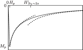
Because of the simplification in Eq. (108), the validity of the result (111) is limited to fields $H\ll H|_{b_{1}\sim 2s}\sim(b^{2}/sW)H_{p}\approx\sqrt{d/s\,}H_{s}$ , where the restriction $s\ll b_{1}$ is satisfied. As shown in Fig. 9, the expression (111) is in good agreement with the numerical solution and describes the evolution of the magnetic response over a large range of fields $H_{p}\lesssim H\ll H|_{b_{1}\sim 2s}$ .

For $b_{1}-s\ll s$ , the same Ansatz $b_{2}=W(1-\nu)^{1/2}$ allows to simplify the constraint Eq. (105) to

\displaystyle b_{1}

\displaystyle=s+W\nu/2,

(112)

while Eq. (107) takes the form

\displaystyle s+W\nu/2

\displaystyle=\sqrt{s^{2}+W^{2}\Big(\frac{H_{p}}{H}\frac{b^{2}}{W^{2}}\Big)^{2}}.

(113)

To leading order in $H_{p}/H$ we find

\displaystyle\nu(H)

\displaystyle=\frac{W}{s}\Big(\frac{H_{p}}{H}\frac{b^{2}}{W^{2}}\Big)^{2}

(114)

and the magnetization reads

\displaystyle M(H)=-\frac{H_{s}^{2}}{4H}Wd.

(115)

For the strongly penetrated double strip, when the current-carrying regions are smaller than $s$ but still wider than $d$ , the mutual influence of the two strips becomes negligible. The magnetization (115) thus approaches that of two independent single strips of width $W$ each [see Eq. (57)].

Pushing the above ‘thin strip’ solution obtained for $s\gg d$ to the limit $s=d$ , we find for the penetration field in Eq. (101)

\displaystyle H_{p}

\displaystyle\approx H_{s}\frac{d}{W}\log{(4W/d)},

(116)

which is substantially smaller than that of an isolated strip as given in Eq. (52). Similarly, in this limit the magnetization as approximated by Eq. (111) becomes

\displaystyle M(H)

\displaystyle=-\frac{H_{s}}{4\pi}4Wd\,\big[\log{(4H_{s}/H)}-1\big].

(117)

This expression is valid for fields up to $H|_{b_{1}\sim 2d}\sim H_{s}$ where the dome reaches the edges and is consistent with the limit $s{\scriptstyle{\ \nearrow\ }}d$ approaching the thickness $d$ from below as discussed in Sec. III below.

In order to understand the penetration mechanism in the double strip for the full range of strip separations $2s$ , below we extend our analysis to a system where the gap width $2s$ is much smaller than the thickness $d$ of the strips, $s\ll d$ , see Sec. III. Before doing that, we briefly elaborate on the corrections due to the vortex structure in the dome.

II.4.3 Magnetization of the vortex dome

To estimate the quantitative effects arising from the currents around the flux lines in the vortex dome, we give an upper bound to the corrections of the magnetic response in Eqs. (111) and (115). Following the analysis presented in Sec. II.3.3, we find an upper bound

\displaystyle\delta M<\frac{H}{4\pi}\frac{H_{c1}}{H_{c1}+H}2Wd

(118)

for the magnetization corrections. In the regime $s\ll W$ the relative correction to the magnetic response is bounded by

\displaystyle\frac{\delta M}{M}

\displaystyle<\frac{H}{H_{s}}\frac{H_{c1}}{H_{c1}+H}\sqrt{\frac{d}{4s}}\frac{1}{\log(4H_{s}/H\sqrt{d/s})-1}

(119)

in the low field range $H<H_{s}\sqrt{d/s}$ [see Eq. (111)] and by

\displaystyle\frac{\delta M}{M}

\displaystyle<\frac{H^{2}}{H_{s}^{2}}\frac{H_{c1}}{H_{c1}+H}\frac{2}{\pi}

(120)

for higher fields field, $H>H_{s}\sqrt{d/s}$ [see Eq. (115)]. The first expression (119) is always small by the order $d/s$ , while the second expression (120) predicts small corrections $\propto(H/H_{s})^{2}$ in the field range $H\ll H_{s}$ , spanning the range of validity for the results presented in this section. We conclude, that the corrections arising due to the vortex state inside the superconducting strips are small, justifying the simplified model for the penetrated state ( $\mu=1$ ) used in our analysis.

III Strips with Finite thickness $\boldsymbol{d}$

III.1 Introduction

We now explore the double strip geometry for narrow gaps $2s\ll d$ . In order to simplify our discussion, the penetration depth $\lambda$ is assumed to be negligible[31], $\lambda\ll s$ . With the gap-width $s$ the smallest geometric length and using $d\ll w$ , the results are presented to leading order in $s/d$ and $d/w$ , respectively; in particular, the half-width $W$ of the system is approximated by the width $2w$ of one strip.

The solutions for infinitely thin strips derived in the previous sections have been regularized near the sample edges with a cut-off $\delta$ of the order of the thickness, $\delta~\sim~d$ . This approach is not appropriate anymore when the spacial solution near (inside) the gap is determined by the length scale $s$ rather than $d$ . The appropriate boundary conditions then have to be taken into account on the entire rectangular cross-section and the strips cannot be treated as infinitely thin anymore.

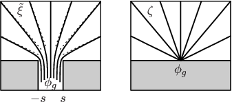
The detailed derivation of the field distribution in the vicinity of the narrow ( $2s$ ) and elongated ( $d$ ) gap (see Fig. 11) presented in Sec. III.2 below will provide us with a uniform field inside the gap of strength

\displaystyle B_{g}

\displaystyle=\frac{\phi_{g}}{2s},

(121)

where the flux $\phi_{g}$ through the gap has to be determined consistently with the field distribution far away from the gap. For distances $s<|\boldsymbol{r}|\ll w$ away from the upper ( $+$ ) and lower ( $-$ ) gap opening, the field assumes the form of a monopole with radial decay

\displaystyle\boldsymbol{B}(\boldsymbol{r})

\displaystyle=\pm\frac{\phi_{g}}{\pi}\frac{\boldsymbol{r}}{|\boldsymbol{r}|^{2}}.

(122)

The corresponding result expressed through the holomorphic field reads

\displaystyle\mathcal{B}(\xi)

\displaystyle=i\,\frac{\phi_{g}}{\pi\xi}.

(123)

In Sec. III.3 we find the field distribution far away from the gap, match the far-field solution with the solution in the gap, and thereby find the flux $\phi_{g}$ through the gap. Along with this derivation, we will discuss the consequences on the double strip solution originating from the current and field distribution in and around the gap.

III.2 Estuary Problem

The field distribution inside the gap and near the opening at $\xi_{{\mathrm{out}}}=0+id/2$ is described by a so-called estuary flow, i.e., the flow into open space of an incompressible fluid leaving a canal of width $2s$ and large (infinite) length $d$ , see Fig. 11. We define the shifted coordinate system $\tilde{\xi}=\xi-\xi_{{\mathrm{out}}}$ centered at the gap opening two-dimensional estuary geometry and determine the holomorphic function $\mathcal{B}(\tilde{\xi})$ . For a diamagnetic superconductor, the field component perpendicular to the surface vanishes everywhere such that $\mathcal{B}(\tilde{\xi})$ is purely real ( $B_{x}=0$ and $B_{z}\neq 0$ ) at the surfaces inside the gap ( $\re{[\tilde{\xi}]}=\pm s$ , $\im{[\tilde{\xi}]}<0$ ) and imaginary ( $B_{x}\neq 0$ and $B_{z}=0$ ) on the surfaces along $x$ , i.e., for $\im{[\tilde{\xi}]}=0$ and $|\!\re{[\tilde{\xi}]}|\geq s$ .

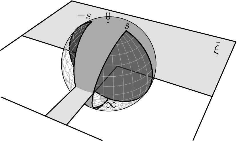
This boundary value problem can be solved with the help of a Schwarz-Christoffel transformation[32] describing a biholomorphic mapping of the upper complex half-plane $\zeta$ , $\im{[\zeta]}\geq 0$ , onto the inner of a polygon. Indeed, the field-allowed region in the estuary geometry is a special case of an unbounded triangle (visualized in Figs. 12 and 13), with vertices $\tilde{\xi}_{v}$ at $-s$ , $-i\infty$ , and $s$ and internal angles $3\pi/2$ , $0$ , and $3\pi/2$ . The corresponding Schwarz-Christoffel transformation takes the form

\displaystyle\tilde{\xi}(\zeta)

\displaystyle=s+\frac{2}{\pi}\bigg[\sqrt{\zeta^{2}-s^{2}}-2s\arctan{\sqrt{\frac{\zeta-s}{\zeta+s}}}\bigg]

(124)

and maps the upper half-plane $\zeta$ (Fig. 11, right) to the estuary plane $\tilde{\xi}$ (Fig. 11, left). The flux $\phi_{g}$ emanating from the vertex at $\tilde{\xi}_{v}=-i\infty$ in the estuary is conserved in the transformation Eq. (124) and maps to a point source of strength $\phi_{g}$ at $\zeta=0$ , with field lines dispersing into the upper half plane $\im[\zeta]\geq 0$ . The complex potential[33]

\displaystyle\bar{\Omega}(\zeta)=\frac{i\phi_{g}}{\pi}\log\zeta

(125)

is generating the field $\mathcal{\bar{B}}(\zeta)=d\bar{\Omega}/d\zeta=i\phi_{g}/\pi\zeta$ of this point source in the upper half-plane. Transforming back to the estuary geometry, the potential $\Omega(\tilde{\xi})=\bar{\Omega}[\zeta(\tilde{\xi})]$ generates the field

\displaystyle\mathcal{B}(\tilde{\xi})=\frac{d\Omega}{d\tilde{\xi}}=\frac{i\phi_{g}}{2}\frac{1}{\sqrt{\zeta(\tilde{\xi})\big.^{2}-s^{2}}}.

(126)

The last equality was obtained by using the Schwarz-Christoffel transformation (124). Alternatively, the analysis on the level of fields involves the solution $\mathcal{\bar{B}}(\zeta)=i\phi_{g}/\pi\zeta$ for a point source and the transformation back involves an additional derivative, $\mathcal{B}(\tilde{\xi})=(d\zeta/d\tilde{\xi})\mathcal{\bar{B}}[\zeta(\tilde{\xi})]$ . In Fig. 11, we show the resulting field lines of Eq. (126) as obtained from inverting Eq. (124) numerically.

In our further discussion it is sufficient to determine the field distribution in the asymptotic regimes where analytic results are available. Deep inside the gap ( $-\im{[\tilde{\xi}]}\gg s$ ) the inverse of Eq. (124) takes the form

\displaystyle\zeta(\tilde{\xi})

\displaystyle=2s\,e^{-[i\pi(\tilde{\xi}-1)/2s]-1}

(127)

and using Eq. (126), we find [up to corrections $\propto\exp({\pi\tilde{z}/2s})$ ] a uniform field directed along $z$ of strength

\displaystyle B_{g}

\displaystyle=\frac{\phi_{g}}{2s}.

(128)

Near the corner of the estuary, $|\tilde{\xi}-s|\ll s$ , the transformation Eq. (124) reads

\displaystyle\frac{\tilde{\xi}-s}{2s}

\displaystyle\sim\frac{2}{3\pi}\left(\frac{\zeta-s}{2s}\right)^{3/2}

(129)

and a similar expression is found near $\tilde{\xi}=-s$ . For both corners, the holomorphic field (126) shows a power law singularity $\propto|\tilde{\xi}\pm s|^{-1/3}$ , which will be regularized in a real sample by the partial penetration (at a depth $\sim s$ ) of vortices into the sample corners.

Far away from the opening, $|\tilde{\xi}|\gg s$ and $\im{[\tilde{\xi}]}\geq 0$ , the inverse transform becomes $\zeta(\tilde{\xi})=\pi\tilde{\xi}/2$ and the holomorphic function (126) assumes the limiting form

\displaystyle\mathcal{B}(\tilde{\xi})

\displaystyle=i\,\frac{\phi_{g}}{\pi\tilde{\xi}}

(130)

describing a point source of strength $\phi_{g}$ located at $\tilde{\xi}=0$ .

III.3 Narrow gap double strip

Away from the gap and from the outer strip edges, a thin-strip description similar to the one discussed in Sec. II is applicable, with the holomorphic field taking the form

\displaystyle\mathcal{B}(\xi)

\displaystyle=H\sqrt{\frac{(\xi^{2}-b_{1}^{2})(\xi^{2}-b_{2}^{2})}{\xi^{2}(\xi^{2}-W^{2})}}.

(131)

The factor $\xi^{2}$ in the denominator [replacing $(\xi^{2}-s^{2})$ in Eq. (30)] captures the flux emanating from the point-like source as derived in Eq. (130). From the above expression, the field distribution along the $x$ -axis is given by

\displaystyle\frac{B_{z}(x)}{H}

\displaystyle=\left\{\begin{aligned} &\sqrt{\frac{(x^{2}-b_{1}^{2})(b_{2}^{2}-x^{2})}{x^{2}(W^{2}-x^{2})}},&&\mathrm{for\ }b_{1}\leq x\leq b_{2},\\ &\sqrt{\frac{(x^{2}-b_{1}^{2})(x^{2}-b_{2}^{2})}{x^{2}(x^{2}-W^{2})}},&&\mathrm{for\ }W\leq x.\end{aligned}\right.

(132)

Comparing Eqs. (130) and (131) in the regime $|\xi|\ll b_{1}$ , we find the flux

\displaystyle\phi_{g}=HW\pi b_{1}b_{2}/W^{2}

(133)

and the uniform field strength (128) inside the gap $|x|<s$ takes the form

\displaystyle B_{g}=H\frac{\pi W}{2s}\frac{b_{1}b_{2}}{W^{2}}.

(134)

Note, that for $s\ll d\ll w$ , the difference between the shifted coordinate $\tilde{\xi}$ and $\xi$ is beyond our resolution, such that $\tilde{\xi}=\xi$ .

The current contribution from the region away from the gap is obtained from the holomorphic field in Eq. (131) via Ampères law (26) and reads

\displaystyle I(x)

\displaystyle=\left\{\begin{aligned} &\frac{Hc}{2\pi}\sqrt{\frac{(b_{1}^{2}-x^{2})(b_{2}^{2}-x^{2})}{x^{2}(W^{2}-x^{2})}},&&s\leq|x|\leq b_{1},\\ &\frac{-Hc}{2\pi}\sqrt{\frac{(x^{2}-b_{1}^{2})(x^{2}-b_{2}^{2})}{x^{2}(W^{2}-x^{2})}},&&b_{2}\leq|x|\leq W,\\ &0,&&\mathrm{otherwise}.\end{aligned}\right.

(135)

The $1/x$ dependence of the current is applicable only for $|x|\gg s$ . However, it turns out that the deviation of $I(x)$ (as obtained from solving Eq. (124) numerically) from $1/x$ is not relevant for the further analysis, and the expression given above for the sheet current density $I(x)$ can be used down to $|x|=s$ .

The homogeneous field (134) inside the gap is generated by a screening current density

\displaystyle j_{g}(x,|z|<d/2)

\displaystyle=\frac{x}{|x|}\frac{B_{g}\,c}{4\pi}\,\delta(|x|-s)

(136)

flowing along $y$ at the gap surfaces ( $x=\pm s$ , $|z|\leq d/2$ ). Here $\delta$ is the Dirac delta function, which accounts for the assumption $\lambda\to 0$ . The two current channels at $x=\pm s$ provide a significant contribution to the total current in the strips. Note that these channels exist for $s\gg d$ as well; for large gaps their contribution to the total current is negligible, though. To treat these currents on equal footing with the sheet current flowing in the strips ( $s\leq x\leq W$ ) we define the sheet current density for the gap currents

\displaystyle I_{g}(x)

\displaystyle=\frac{x}{|x|}\frac{B_{g}c}{4\pi}\,d\,\delta(|x|-s)

(137)

by integrating Eq. (136) over the strip thickness $d$ .

The currents flowing along the vertical surfaces at the outer edges ( $|x|=W$ ) are parametrically smaller as compared to the contributions near the gap ( $|x|=s$ ) and are neglected here. The two dominant current contributions then add up to the total current, $I_{\mathrm{tot}}(x)=I(x)+I_{g}(x)$ . This current distribution, when compared to the thin strip case, corresponds to a rearrangement of the current densities towards the inner edges of the strips, see Fig. 14.

The diamagnetic contribution from the current $I(x)$ in the strip,

\displaystyle M(H)

\displaystyle=-\frac{H}{4}(W^{2}-b_{1}^{2}-b_{2}^{2}),

(138)

as obtained from evaluating Eq. (43) with the field (131), is parametrically larger ( $\propto W/d$ ) than the paramagnetic contribution

\displaystyle M_{g}(H)

\displaystyle=\frac{H}{4}W^{2}\frac{b_{1}b_{2}d}{W^{3}}

(139)

from the current $I_{g}(x)$ along the gap surface and we neglect the latter in the following. The problem is then, once again, reduced to finding the parameters $b_{1}$ and $b_{2}$ within the Meissner- and penetrated states.

III.3.1 Meissner state

In the Meissner state were $b_{1}=b_{2}=b$ , the field $B_{z}$ [Eq. (131)] along the $x$ -axis simplifies to

\displaystyle B_{z}(x)

\displaystyle=H\frac{x^{2}-b^{2}}{|x|\sqrt{x^{2}-W^{2}}}.

(140)

for $|x|>W$ and is constant [Eq. (134)],

\displaystyle B_{g}=H\pi\frac{b^{2}}{2sW},

(141)

inside the gap ( $|x|<s$ ). The total sheet current density reads

\displaystyle I_{\mathrm{tot}}(x)

\displaystyle=-\frac{Hc}{2\pi}\bigg[\frac{x^{2}-b^{2}}{x\sqrt{W^{2}-x^{2}}}-\frac{x}{|x|}\frac{\pi b^{2}}{4sW}\,d\,\delta(|x|-s)\bigg]

(142)

and the general expression (138) for the magnetization takes the form

\displaystyle M(H)

\displaystyle=-\frac{H}{4}(W^{2}-2b^{2}).

(143)

The value of the parameter $b$ is fixed by the constraint of vanishing net current given as

\displaystyle\int\limits_{s}^{W}\frac{dx\,x}{\sqrt{W^{2}-x^{2}}}=b^{2}\bigg[\frac{\pi d}{4sW}+\int\limits_{s}^{W}\frac{dx}{x\sqrt{W^{2}-x^{2}}}\bigg].

(144)

The above integrals simplify in the limit $s\ll W$ and the parameter $b$ takes the asymptotic form

\displaystyle b^{2}

\displaystyle=\frac{W^{2}}{\pi d/4s+\log\big(2W/s\big)}.

(145)

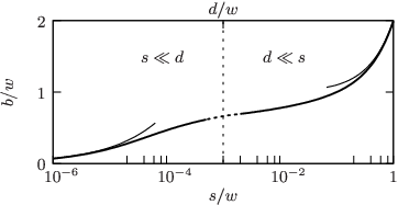
In contrast to the result for thin strips [see Eq. (93)], where $b^{2}$ changes logarithmically with $s$ , in the present case the dependence on $s$ is dominated by the linear term $d/s$ in the denominator. As a result, the parameter $b$ is substantially reduced when $s\ll d$ , see Fig. 15, which is due to the additional currents $I_{g}$ flowing at the (vertical) gap surface and producing a substantial rearrangement of the overall current density as shown in Fig. 14.

We note that the numerical factor $\pi/4$ of the term $d/s$ in the above expression is precisely known since it derives from the current $I_{g}(x)$ originating from screening the uniform field inside the gap, Eq. (137). The prefactor under the logarithm, however, will be modified if the field distribution at the opening of the estuary is accurately taken into account. Indeed, approaching the corner $(s,d/2)$ from both surfaces $(x,d/2)$ and $(s,z)$ the field deviates from the assumed behavior $B_{x}(x)\propto 1/x$ and $B_{z}(z)=\mathrm{const}$ [following from Eqs. (131) and (134) respectively]. The precise field distribution (and its related current profile) can be derived by solving Eq. (124) numerically and inserting the result into Eq. (126). Neglecting partial penetration of the edge corners, Eq. (145) will be modified to

\displaystyle b^{2}

\displaystyle=\frac{W^{2}}{\pi d/4s+\log\big(2.38W/s\big)}.

(146)

Since the precision of this expression also suffers from corrections (e.g. from partial penetration of the edge corners), we will use the relation (145) in the following.

The diamagnetic response in the Meissner phase follows from (143) and reduces to

\displaystyle M(H)

\displaystyle\approx-\frac{H}{4}W^{2}\bigg[1-\frac{8s/\pi d}{1+(4s/\pi d)\log\big(2W/s\big)}\bigg].

(147)

This result approaches that of a single strip of double width [cf. Eq. (51) with $w\to W$ ] upon reducing $s$ far below $d$ .

Using Eq. (145) in the expression (133) for the flux through the gap, we find that

\displaystyle\phi_{g}

\displaystyle=H2W\frac{2s/d}{1+(4s/\pi d)\log\big(2W/s\big)}

(148)

shrinks (up to logarithmic corrections) linearly with decreasing $s$ (note that $b_{1}b_{2}=b^{2}$ ). Compared to the blocked flux $\phi_{b}\approx H\,2W$ , only a small fraction $\sim 2s/d$ passes through the narrow gap of width $2s$ and length $d$ . Consequently, the field strength inside the gap,

\displaystyle B_{g}=H\frac{2W}{d}\frac{1}{1+(4s/\pi d)\log\big(2W/s\big)},

(149)

does not diverge for $s/d\to 0$ but saturates at $H\,2W/d$ .

As the field profile inside the gap from where vortices start penetrating the sample is precisely known, the present penetration process is more accurately described than the one for the thin-strip limit where the strips are separated by a distance larger than $d$ . Corrections originating from the precise field distribution near the opening of the estuary affect the results only to the next-to-leading order.

As before, the penetration starts when the field inside the gap reaches the strength $H_{s}$ , i.e., at the penetration field

\displaystyle H_{p}

\displaystyle=H_{s}\frac{2s}{\pi W}\frac{W^{2}}{b^{2}}=H_{s}\frac{d}{2W}\Big[1+\frac{4s}{\pi d}\log\Big(\frac{2W}{s}\Big)\Big].

(150)

In the limit $s/d\to 0$ , the penetration field asymptotically reaches the value $H_{s}d/2W$ , that is the penetration field of the elliptic strip, cf. Eq. (15). The retardation of field penetration originating from the geometrical barrier has completely disappeared in this limit. At penetration, $H=H_{p}$ , the diamagnetic response

	$\displaystyle M_{p}$	$\displaystyle=-\frac{H_{s}}{16}(2Wd)\Big\{1+\frac{2s}{\pi d}\Big[2\log\Big(\frac{2W}{s}\Big)-1\Big]\Big\}$		(151)
		$\displaystyle=-\frac{H_{p}}{4}W^{2}\Big[1-\frac{8s/\pi d}{1+(4s/\pi d)\log\big(2W/s\big)}\Big],$		(152)

has collapsed by a factor $\sim(d/W)^{1/2}$ as compared to that of a single strip, Eq. (53), for which the geometrical barrier is fully active. This so-called ‘suppression of the geometrical barrier’, the collapse of $H_{p}$ and of $M(H)$ , is a central result of this work. Although in the limiting case $s/d\to 0$ , the Meissner response and the field of first penetration coincide with that of an elliptically shaped strip, beyond $H_{p}$ , the magnetic signatures of the double strip still differs substantially from those of the elliptic sample, see Figs. 16 and 17 as well as the discussion below.

Upon decreasing the gap width $s$ , the penetration field $H_{p}$ is reduced, what leads to a stronger suppression of the geometrical barrier as follows from Eq. (36). The calculation of the equilibrium field defined through Eq. (37) provides the result

\displaystyle H_{\mathrm{eq}}=H_{c1}\frac{d}{2W}\Big[1-\frac{\log(W^{2}/b^{2})-1}{\pi d/2s+\log(4W^{2}/s^{2})}\Big]^{-1},

(153)

approaching $H_{c1}d/2W$ and the corresponding geometrical barrier height (38) vanishes as $s\log(s)$ ,

	$\displaystyle U_{b}^{\mathrm{eq}}$	$\displaystyle=\varepsilon_{l}d\Big(1-\Big\{1+\frac{2s}{\pi d}\big[\log(4b^{2}/s^{2})-1\big]\Big\}^{-1}\Big)$		(154)
		$\displaystyle\approx\varepsilon_{l}d\ \frac{2s}{\pi d}\big[\log(16W^{2}/\pi sd)-1\big],$		(155)

where we have assumed that $s\log(W/s)\ll d$ for the last equality.

III.3.2 Penetrated state

The field and current distributions Eqs. (131), (134) and Eqs. (135), (137) describe the penetrated state once the parameters $b_{1}$ and $b_{2}$ have been found; the latter have to respect the limits $b_{1}-s\gg s$ and $W-b_{2}\gg d$ and are determined by the usual conditions governing the evolution of the vortex dome, the vanishing of the total currents in the strips,

\displaystyle\int\limits_{s_{-}}^{b_{1}}dx\,I_{\mathrm{tot}}(x)+\int\limits_{b_{2}}^{W}dx\,I_{\mathrm{tot}}(x)

\displaystyle=0

(156)

and the condition of criticality at the edge regulating the vortex entrance, here $B_{g}=H_{s}$ . The latter condition is equivalent to the requirement that the flux $\phi_{g}$ in (133) saturates at $H_{s}2s$ , or

\displaystyle\frac{b_{1}b_{2}}{b^{2}}

\displaystyle=\frac{H_{p}}{H},

(157)

as expressed through the penetration field $H_{p}$ and the zero-current position $b$ of the Meissner state.

As before, the perturbative calculation around the penetration field $H_{p}$ is very limited due to the rapid growth of the dome width $b_{2}-b_{1}$ beyond $H_{p}$ and we concentrate on the high-field expansion where the vortex domes occupy a large fraction of the strips $b_{1}\ll b_{2}$ , providing results over a large field-range. The two conditions regulating the dome evolution then can be simplified and an analytic solution can be given. With the Ansatz $b_{2}=W(1-\nu)^{1/2}$ with $\nu<1$ , the inner dome edge

\displaystyle b_{1}

\displaystyle=\frac{b^{2}}{W}\frac{H_{p}}{H}\frac{1}{\sqrt{1-\nu}}

(158)

is expressed through $\nu$ with the help of Eq. (157). Assuming $s\ll b_{1}$ and $b_{1}\ll b_{2}$ , the requirement of vanishing net current in Eq. (156) simplifies to

	$\displaystyle\frac{H_{p}}{H}\frac{b^{2}}{W^{2}}\left[\frac{W^{2}}{b^{2}}+\log{\Big(\frac{b^{2}}{W^{2}}\frac{H_{p}}{H}\frac{1}{\sqrt{1-\nu}}\Big)}-1\right]$			(159)
	$\displaystyle=\E(\sqrt{\nu})-(1$	$\displaystyle-\nu)\K(\sqrt{\nu}).$

For large fields $H\gg H_{p}$ , where $\nu$ is small, the above equation can be expanded in $\nu$ . Solving for $\nu(H)$ to second order in $H_{p}/H$ , we obtain

$\displaystyle\nu(H)$	$\displaystyle\approx\frac{4}{\pi}\frac{H_{p}}{H}\bigg\{1+\frac{b^{2}}{W^{2}}\bigg[\log{\left(\frac{b^{2}}{W^{2}}\frac{H_{p}}{H}\right)}-1\bigg]\bigg\}$	(160)
	$\displaystyle\ -\frac{2}{\pi^{2}}\frac{H_{p}^{2}}{H^{2}}\bigg\{1+\frac{b^{2}}{W^{2}}\bigg[\log{\bigg(\frac{b^{2}}{W^{2}}\frac{H_{p}}{H}\bigg)}-1\bigg]\bigg\}^{2}$
	$\displaystyle\ +\frac{8}{\pi^{2}}\frac{H_{p}^{2}}{H^{2}}\frac{b^{2}}{W^{2}}\bigg\{1+\frac{b^{2}}{W^{2}}\bigg[\log{\bigg(\frac{b^{2}}{W^{2}}\frac{H_{p}}{H}\bigg)}-1\bigg]\bigg\}.$

The magnetic response given in Eq. (138) simplifies to $M(H)=-H\nu(H)W^{2}/4$ and Fig. 16 shows the result of combining this expression with $\nu(H)$ from Eq. (160). Although the range of applicability $H_{p}\ll H$ of the above expression does not a-priori cover the regime near penetration, the results are still in good agreement with the numerical solution down to $H\approx H_{p}$ .

Neglecting irrelevant terms of order $(b/W)^{2}(H_{p}/H)^{2}$ and higher in Eq. (160), the magnetization reads

\displaystyle M(H)

\displaystyle\approx\bar{M}\bigg\{1+\frac{b^{2}}{W^{2}}\bigg[\log{\bigg(\frac{b^{2}}{W^{2}}\frac{H_{p}}{H}\bigg)}-1\bigg]-\frac{1}{2\pi}\frac{H_{p}}{H}\bigg\},

(161)

with $\bar{M}=-H_{p}W^{2}/\pi$ . In contrast to the thin strip case [see Eq. (111)], where the magnetization depends logarithmically $\propto\log{(H_{s}/H)}$ on the applied field, the magnetic response in the present limit is dominated by a field-independent contribution,

\displaystyle\bar{M}

\displaystyle\approx-\frac{H_{p}}{\pi}W^{2}\approx-\frac{H_{s}}{4\pi}(2Wd),

(162)

producing an almost flat magnetization. This flatness is the result of the particular current distribution inside the strips: The current flowing close to the inner edge is dominated by the contribution $I_{g}(x)$ from the gap, i.e.,

\displaystyle\int\limits_{s_{-}}^{b_{1}}dx\,I_{\mathrm{tot}}(x)

\displaystyle\approx\int\limits_{s_{-}}^{s_{+}}dx\,I_{g}(x)=\frac{H_{s}c}{4\pi}\,d.

(163)

To satisfy the condition (156) of vansihing net current, the current density $I(x)$ between $b_{2}$ and $W$ has to compensate the gap contribution, leading to

\displaystyle\int\limits_{b_{2}}^{W}dx\,I_{\mathrm{tot}}(x)

\displaystyle\approx-\frac{H_{s}c}{4\pi}\,d.

(164)

Once the dome occupies a large fraction of the sample, these currents flow at the outer edge, i.e., a distance $\sim W$ away from the origin and produce the dominant (field-independent) contribution $-H_{s}(2Wd)/4\pi$ [cf. Eq. (162)] to the magnetization at large fields (the factor 2 originates from the integration over both strips). Note that in the limit $s/d\to 0$ , the leveling out of the magnetization at the value given in Eq. (162) is by a factor $4/\pi$ larger than its value at penetration $H_{p}$ [see Eq. (151)].

Although almost constant, the magnetization (161) assumes a maximal diamagnetic signal

\displaystyle M(H_{m})

\displaystyle=\bar{M}\bigg\{1+\frac{4s}{\pi d}\bigg[\log\bigg(\frac{32s^{2}}{\pi d^{2}}\bigg)-2\bigg]\bigg\}

(165)

at the applied field

\displaystyle H_{m}

\displaystyle\approx H_{p}\frac{d}{8s}\approx\frac{H_{s}}{16}\frac{d^{2}}{sW}.

(166)

For $s/d\lesssim d/16W$ , the diamagnetic response monotonically increases up to $H\sim H_{s}$ . On the other hand, we may extrapolate the expression (166) to $s\lesssim d$ and predict a value of the gap parameter $s\sim d/8$ where $H_{m}$ merges with the penetration field $H_{p}$ upon increasing $s$ . The “flatness” of the magnetization curve in the penetrated state is quantified by relating the slope $M^{\prime}(H)$ [as obtained from Eq. (161)] to the Meissner slope $-W^{2}/4$ , yielding

\displaystyle-\frac{4M^{\prime}(H)}{W^{2}}=\frac{2}{\pi^{2}}\bigg(\frac{H_{p}^{2}}{H^{2}}-\frac{8s}{d}\frac{H_{p}}{H}\bigg)\ll 1.

(167)

As for thin strips and wide gaps (see Sec. II.4.2), we can push the results obtained in the limit $s\ll d$ to the extreme case $s\to d$ . The penetration field

\displaystyle H_{p}

\displaystyle\approx H_{s}\frac{d}{2W}\Big[1+\frac{4}{\pi}\log\Big(\frac{2W}{d}\Big)\Big]

(168)

as obtained from Eq. (150) with $s=d$ , agrees up to numbers of order unity with the result obtained from the opposite limit $s\gg d$ , see Eq. (116). Taking the limit $s\to d$ from the regime of small gaps $s\ll d$ , the magnetization is dominated by the first term in Eq. (160) and simplifies to

\displaystyle M(H)

\displaystyle\approx-\frac{H_{s}}{4\pi}(4Wd)\Big[\frac{2}{\pi}\log{\Big(\frac{4H_{s}}{\pi H}\Big)}+\frac{4-\pi}{2\pi}\Big].

(169)

This expression agrees well with the corresponding expression (117) obtained in the limit $s{\scriptstyle{\ \searrow\ }}d$ approaching the thickness $d$ from above.

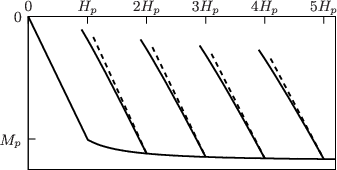
Although the penetration field (150) asymptotically ( $s/d\to 0$ ) approaches the equilibrium field (153), a finite irreversibility persists and the geometric barrier rapidly reappears upon reducing the applied field. Upon decreasing the magnetic field from a maximal value $H^{\star}$ , the vortex dome expands while keeping the trapped flux constant,

\displaystyle\phi_{d}(H)

\displaystyle\equiv\int\limits_{b_{1}}^{b_{2}}dx\,H\sqrt{\frac{(x^{2}-b_{1}^{2})(b_{2}^{2}-x^{2})}{x^{2}(W^{2}-x^{2})}}=\phi_{d}^{\star},

(170)

where $\phi_{d}^{\star}=\phi_{d}(H^{\star})$ . This constraint for the decreasing field replaces the constraint $B_{g}=H_{s}$ for the increasing field. Excluding a narrow field range $H^{\star}\simeq H_{p}$ , the dome extends over a large fraction of the sample and the constraint of conserved trapped flux can be simplified under the assumptions $b_{1}\ll b_{2}$ and $W-b_{2}\ll W$ to read

\displaystyle HW\Big\{1-\frac{\nu}{4}\Big[\log\Big(\frac{16}{\nu}\Big)+1\Big]\Big\}

\displaystyle=\phi_{d}^{\star},

(171)

where we used $\nu(H)=1-[b_{2}(H)/W]^{2}\ll 1$ as before. Similar to the single strip calculations [see Eq. (73)], the slope of the magnetic response $M(H)=-H\nu(H)W^{2}/4$ is given by

\displaystyle\frac{dM}{dH}

\displaystyle=-\frac{W^{2}}{4}\frac{4-\nu}{\log(16/\nu)},

(172)

which is numerically close to that of the Meissner phase ( $-W^{2}/4$ ). At the onset of the descending branch, i.e., $H^{\star}-H\ll H^{\star}$ , we find an analytic expression for the magnetization of the form

\displaystyle M(H)=M(H^{\star})-\frac{H-H^{\star}}{4}W^{2}\frac{4-\nu^{\star}}{\log(16/\nu^{\star})},

(173)

where $\nu^{\star}=\nu(H^{\star})$ is obtained from Eq. (160). The above expression and the result of an exact numerical calculation of the magnetization are shown in Fig. 17.

III.3.3 Magnetization of the vortex dome

In the limit $s\ll d$ , the diamagnetic response of the double strip is flat and small by the factor $\sim\sqrt{d/W}$ as compared to the single strip at $H_{p}$ ; hence, we should verify that the magnetic response of the vortex state in the flux-filled region does not substantially alter the above results. Following again the analysis discussed earlier in Sec. II.3.3, the corrections to the magnetic response (162) are bounded from above by the function

\displaystyle\delta M<\frac{H}{4\pi}\frac{H_{c1}}{H_{c1}+H}2Wd

(174)

leading to relative corrections

\displaystyle\frac{\delta M}{M}

\displaystyle<\frac{H}{H_{s}}\frac{H_{c1}}{H_{c1}+H}\frac{4}{\pi}

(175)

that are small as long as $H\ll H_{s}$ . Without surface barrier, $H_{s}=H_{c1}$ , the corrections become of order unity only when $H\sim H_{c1}$ . On the other hand, for a large surface barrier $H_{s}\gg H_{c1}$ , the corrections remain small when $H\sim H_{s}$ . We conclude, that the contribution of the equilibrium magnetization of the Shubnikov state to the overall magnetization of the double strip geometry (with $s\ll d\ll w$ ) is small and can, in most cases, be neglected in the entire field range $H<H_{c1}$ .

IV Several strips

So far, we have given a detailed description of the single and double strip geometries. A discussion of three coplanar strips will reveal additional features as compared to the previous systems, and allows for a qualitative understanding of the response of a system of a finite number $n\geq 3$ of coplanar strips in a parallel arrangement.

The general holomorphic field for $n$ ( $n\geq 1$ ) parallel strips arranged symmetrically around the origin $\xi=0$ assumes the form

\displaystyle\mathcal{B}(\xi)

\displaystyle=H\sqrt{\prod\limits_{i}\frac{\xi^{2}-b_{i}^{2}(H)}{\xi^{2}-e_{i}^{2}}},

(176)

where $\pm e_{i}$ denote the strip edges and the parameters $b_{i}(H)$ define the boundaries of the vortex states. For an even number $n=2m$ of strips, the $k$ th strip ( $0<k\leq m$ ) as counted along the positive $x$ -axis ranges from $e_{2k-1}$ to $e_{2k}$ and vortices fill the region $b_{2k-1}$ to $b_{2k}$ . Every strip has a symmetric counterpart on the negative $x$ -axis. For an odd number $n=2m+1$ of strips, the above remains unchanged except for an additional innermost strip ranging from $-e_{0}$ to $e_{0}$ with a dome between $-b_{0}$ and $b_{0}$ . The product in Eq. (176) runs from 1 to $n$ (from 0 to $n-1$ ) for the even (odd) numbered configurations. The expressions (29) and (30) are special cases for the single and double strip geometries. The magnetization of the $n$ -strip system as obtained from Eq. (43) reads

\displaystyle M(H)

\displaystyle=-\frac{H}{4}\sum\limits_{i}(e_{i}^{2}-b_{i}^{2}).

(177)

In this section, we consider strips of equal width $2w$ and separated by a gap $2s$ . We also limit the analysis to the thin strip case, i.e., the thickness $d$ of the strips is the smallest of all geometric lengths.

IV.1 Three strips

The holomorphic field for three parallel strips reads

\displaystyle\mathcal{B}(\xi)

\displaystyle=H\sqrt{\frac{[\xi^{2}-b_{0}^{2}(H)][\xi^{2}-b_{1}^{2}(H)][\xi^{2}-b_{2}^{2}(H)]}{(\xi^{2}-e_{0}^{2})(\xi^{2}-e_{1}^{2})(\xi^{2}-e_{2}^{2})}},

(178)

with $e_{0}=w$ , $e_{1}=w+2s$ , and $e_{2}=3w+2s$ .

IV.1.1 Meissner state

For small fields, where the entire system is in the Meissner state, i.e., no vortices have penetrated in either of the strips, the holomorphic field reduces to

\displaystyle\mathcal{B}(\xi)

\displaystyle=H\sqrt{\frac{\xi^{2}(\xi^{2}-b^{2})^{2}}{(\xi^{2}-e_{0}^{2})(\xi^{2}-e_{1}^{2})(\xi^{2}-e_{2}^{2})}},

(179)

where the remaining parameter $b$ ( $=b_{1}=b_{2}$ , note that $b_{0}=0$ ) is determined from requiring a vanishing total current in the outer strip pair,

	$\displaystyle\int\limits_{e_{1}}^{e_{2}}$	$\displaystyle\frac{dx\,x\,b^{2}}{\sqrt{(x^{2}-e_{0}^{2})(x^{2}-e_{1}^{2})(e_{2}^{2}-x^{2})}}$		(180)
		$\displaystyle\quad\qquad\qquad\qquad=\int\limits_{e_{1}}^{e_{2}}\frac{dx\,x^{3}}{\sqrt{(x^{2}-e_{0}^{2})(x^{2}-e_{1}^{2})(e_{2}^{2}-x^{2})}}.$

With the substitution $x^{2}\to e_{1}^{2}+(e_{2}^{2}-e_{1}^{2})t^{2}$ the solution can formally be expressed through

\displaystyle b^{2}

\displaystyle=e_{0}^{2}+(e_{1}^{2}-e_{0}^{2})\frac{\E(\kappa)}{\K(\kappa)},

(181)

where the elliptic integrals, defined in Eqs. (61) and (62), are evaluated at the imaginary argument $\kappa=\sqrt{(e_{2}^{2}-e_{1}^{2})/(e_{0}^{2}-e_{1}^{2})}$ , $\kappa^{2}<0$ . In two asymptotic regimes the above result simplifies to

\displaystyle b^{2}

\displaystyle\simeq\left\{\begin{aligned} &4(w+s)^{2}&\mathrm{for\ }s\gg w,\\ &w^{2}\Big[1+\frac{16}{\log{(32w/s)}}\Big]&\mathrm{for\ }s\ll w.\\ \end{aligned}\right.

(182)

The first limit ( $s\gg w$ ) describes three almost isolated strips, while in the latter case of nearby strips with $s\ll w$ a logarithmic dependence of $b$ on $s$ shows up, analogous to the expression (93) for two strips. Focusing on the regime of nearby strips $s\ll w$ , we find that the flux

\displaystyle\phi_{g}

\displaystyle=\int\limits_{e_{0}}^{e_{1}}\!dx\,B_{z}(x)\approx H6w\frac{\pi\sqrt{2}}{3}\frac{1}{\log{(32w/s)}}

(183)

passing through each of the two gaps carries a substantial fraction of the flux $\phi_{\mathrm{b}}=H6w$ that is blocked by the strips. The field enhancement $\sim H\sqrt{w^{2}/sd}$ at the strip edges $e_{0}$ and $e_{1}$ [see Eq. (179)] is found to be parametrically $\sim\sqrt{w/s}$ larger than at the outermost edge $e_{2}$ . A more detailed calculation reveals, that the field strength is largest near $e_{0}$ , followed by a slightly lower field near $e_{1}$ ,

\displaystyle\frac{B_{z}(e_{1}-d/2)}{B_{z}(e_{0}+d/2)}=1-\frac{21w^{2}-5b^{2}}{b^{2}-w^{2}}\frac{s}{4w}.

(184)

We conclude that the critical field $H_{s}$ [as discussed in Eq. (35)] is first reached at the edges $\pm e_{0}$ (strip index $k=0$ ) where the field enhancement is most pronounced. Thus, the geometrical barrier is first suppressed in the central strip and vortices start to penetrate the innermost strip beyond

\displaystyle H_{p}^{k=0}

\displaystyle\approx H_{s}\sqrt{\frac{sd}{8w^{2}}}\log(32w/s).

(185)

This critical field is parametrically similar to the field of first penetration of the double strip geometry, see Eq. (101).

IV.1.2 Penetrated state(s)

In general, for a multiple strip geometry, the strips are not equivalent and the penetration of vortices starts at a different field value for each strip. The penetration sequence may depend on the geometrical setup as well as on the boundary condition at $y\to\pm\infty$ (shunted vs. unshunted ends). In particular, we shall compare our results to the findings by Mawatari et al., who considered a system of three shunted strips in Ref. [21]. As the external field $H$ increases beyond $H_{p}^{k=0}$ , vortices populate the innermost strip ( $b_{0}\neq 0$ ), while the two other strips remain free of flux ( $b_{1}=b_{2}=b$ ). The field distribution then is given by

\displaystyle\mathcal{B}(\xi)

\displaystyle=H\sqrt{\frac{(\xi^{2}-b_{0}^{2})(\xi^{2}-b^{2})^{2}}{(\xi^{2}-e_{0}^{2})(\xi^{2}-e_{1}^{2})(\xi^{2}-e_{2}^{2})}},

(186)

where the two parameters $b_{0}$ and $b$ (now both depending on $H$ ) are fixed by the constraints of critical field strength $H_{s}$ near the edge $e_{0}$ and vanishing net current

\displaystyle\int\limits_{e_{1}}^{e_{2}}dx\,I(x)=0

(187)

in the outer strips. The outer strip pair will first be penetrated by vortices only at a higher field $H_{p}^{k=1}$ , where a critical field strength $H_{s}$ is reached at the edge $e_{1}$ . At this particular field, the requirement that the field strength is critical at both edges $e_{0}$ and $e_{1}$ while the outer dome has not yet developed ( $b_{1}=b_{2}=b$ ), gives a relation between $b_{0}$ and $b$ of the form

\displaystyle b_{0}^{2}

\displaystyle=w^{2}\Big[1-\frac{8(b^{2}-w^{2})}{16w^{2}+5(b^{2}-w^{2})}\Big].

(188)

Inserting this relation $b_{0}(b)$ into the constraint (187) of vanishing net current in the outer strip fixes the last degree of freedom $b$ and permits to express the second penetration field through

\displaystyle H_{p}^{k=1}

\displaystyle=H_{s}\sqrt{\frac{32w^{4}sd}{(w^{2}-b_{0}(b)^{2})(b^{2}-w^{2})^{2}}}.

(189)

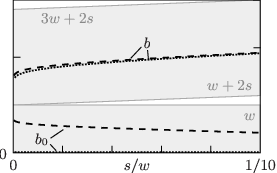
Solving Eqs. (187) and (188) numerically, we show the results for the two penetration fields $H_{p}^{k=0}$ and $H_{p}^{k=1}$ in Fig. 18. Using the same numerical solution, we visualize in Fig. 19 the dome boundaries $b_{0}$ and $b$ within the strips at the first (second) penetration field $H_{p}^{k=0}$ ( $H_{p}^{k=1}$ ) for different values of the gap width $2s$ . We observe that $b(H)$ changes only little between $H_{p}^{k=0}$ and $H_{p}^{k=1}$ . This finding allows us to give an estimate for $H_{p}^{k=1}$ ; indeed, inserting $b(H_{p}^{k=1})\approx b(H_{p}^{k=0})$ in Eq. (189) where $b(H_{p}^{k=0})$ is taken from Eq. (182), we find

\displaystyle\frac{H_{p}^{k=1}}{H_{p}^{k=0}}

\displaystyle\approx\sqrt{\frac{w^{2}}{w^{2}-b_{0}(b)^{2}}}\approx\sqrt{\frac{5+\log(32w/s)}{8}}.

(190)

Beyond $H_{p}^{k=1}$ , all three strips are penetrated, and the dome widths are determined by the restriction of no net current in the outer strips and the two critical field conditions at the edges $e_{0}$ and $e_{1}$ . Note, that the central strip is penetrated from both edges while the strips of the pair $k=1$ are penetrated from the inner edges $\pm e_{1}$ only.

The order in which the strips are populated with vortices depends on the specification of the problem. Indeed, if the same geometrical configuration was shunted at both ends ( $y\to\pm\infty$ ), as considered in Ref. [21], the outer strip pair would be populated by vortices from $\pm e_{2}$ , while the innermost strip remains free of flux until much higher fields.

IV.2 Many strips - General picture

For any finite number of unshunted strips, the field enhancement in the Meissner state is strongest at the innermost edges, i.e., the inner edges at $\pm e_{1}$ for an even number of strips and the two edges at $\pm e_{0}$ of the central strip for an odd number of strips (the only case where a strip is penetrated from both sides). Subsequently, the strips are always penetrated asymmetrically from the inner edges. Specifically, when the applied field is raised beyond the first penetration field, vortices start to populate the innermost strip(s) through the respective edges, while all other strips are still free of flux. Under further increase of $H$ , the critical field strength $H_{s}$ is successively reached at the inner strip edges $e_{2k-1}$ and vortices penetrate the strip pair $k$ , when $H>H_{p}^{k}$ , with $H_{p}^{k}>H_{p}^{k-1}$ , with $k$ starting from 1 (2) in the case of an odd (even) number of strips. In the limit of a large number of strips, the field strengths in the different gaps are almost the same, such that vortex penetration starts within a narrow field range in all the strips.

V Summary and Conclusions

In summary, we have investigated the magnetic response of (two) aligned superconducting strips subject to a perpendicular magnetic field $H$ . The penetration of vortices in these systems is dominated by a macroscopic energy barrier, the so-called geometrical barrier. We have found that a narrow slit between the strips completely suppresses this geometrical barrier as manifested in an early field penetration and the collapse of the hysteretic magnetization loop. We have compared the results for a pair of rectangular (platelet shaped) strips to those of various other shapes and geometries. Of particular interest is the comparison with a single elliptic strip, i.e., the generic shape defining demagnetization effects, and a single platelet strip, the simplest system exhibiting a geometric barrier. In the elliptic case, vortices penetrate the sample above a field $H_{p}=H_{s}d/2w$ ( $H_{c1}\leq H_{s}<H_{c}$ ), distribute uniformly inside the sample, and produce a reversible response (in the absence of a surface barrier). The penetration of vortices in a platelet sample is impeded by a geometrical energy barrier (and potentially an additional surface barrier) at the sample edges, $H_{p}=H_{s}\sqrt{d/w}$ . Once this barrier is overcome, vortices occupy a finite region inside the sample (vortex dome), while the rest carries the diamagnetic shielding currents. Upon decreasing the applied field, the strip shows a irreversible response, where the penetrated flux is trapped inside the sample until the vortex dome expands to the sample edges. These qualitative features remain valid for an array of rectangular strips.

The attention of the present work has mainly focused on the double strip. In the regime of a small gap parameter $s\ll w$ , where the strip system is equivalent to a single strip of width $2W=4w+2s$ cut in half by a narrow gap, the geometrical barrier is overcome at much lower applied fields $H$ . When $d$ is the smallest geometric length, the situation still resembles the one of the single strip; modifications concern the field of first penetration, $H_{p}=H_{s}\sqrt{d/W}\boldsymbol{[}\sqrt{s/W}\log(4W/s)\boldsymbol{]}$ , the exclusive penetration from the inner edges, and the asymmetric shape of the vortex domes leaning towards the gap. When the gap width $2s$ drops below the thickness $d$ , the currents rearrange strongly, piling up at the inner surfaces and channeling a larger field through the central opening. In the limit $s/d\to 0$ , the geometrical barrier is maximally suppressed and the penetration field $H_{p}=H_{s}d/2W$ of the double strip coincides with that of a single ellipse with aspect ratio $d/2W$ . In contrast to the previously discussed cases where the magnetization decreases beyond penetration, here the magnetic response levels off at the magnitude $M=H_{s}Wd/2\pi$ , a factor $4/\pi$ above the magnetization at the penetration field.

In order to study the irreversibility due to the geometric barrier, we have examined the descending branch in the magnetization upon reduction of the field. Remarkably, our analytic results show, that the initial slope of the descending branch is close to the Meissner response, with a correction factor approaching unity when the reversing field approaches $H_{p}$ from above; reversing the field at larger $H$ , the Meissner slope is changed by a factor $(4-\nu)/\log(16/\nu)$ , where $\nu$ depends only on the point $(H,M)$ where the slope is evaluated, $\nu=-4M/Hw^{2}$ . Surprisingly, the correction factor remains close to unity over a wide range of $\nu<1$ . The latter result is equally valid for both the single and narrow-gap ( $s\ll d$ ) double strip.

In addition, we have examined the influence of the vortex currents in the Shubnikov phase; while our complex-analysis approach describes the vortex-phase in terms of a non-magnetic medium, it intrinsically exhibits a finite magnetic response. We have shown that the magnetization due to the structure of the vortex state in the dome remains small within the region $H<H_{s}$ where our analysis is valid. Finally, we have extended our analysis to $n$ ( $\geq 3$ ) strips and have given a qualitative discussion of the field penetration for this more complex geometry.

The suppression of the geometrical barrier can be beneficial in many circumstances, as the hysteretic behavior due to geometrical effects often obscures other interesting physical phenomena. E.g., this has been the case in the identification of the vortex-lattice melting-transition in platelet-shaped layered BiSCCO samples, where the irreversibility line potentially interferes with the first-order melting line: polishing the sample into a prism shape, the geometrical barrier could be suppressed, what allowed to demonstrate experimentally that melting and irreversibility are uncorrelated phenomena [6]. Another example is the competition between bulk pinning of vortices and pinning due to surface- and shape effects as analyzed in the present work: again, the suppression of the geometrical barrier provides access to an unambiguous study of bulk pinning phenomena. In evaluating different means to suppress the geometrical barrier, the generation of a simple gap or crack in the sample appears as a rather simple alternative. Recently, the suppression of geometrical barriers in platelet BiSCCO samples has also been observed when tilting the magnetic field [7]. This finding has been related to the appearance of Josephson vortex stacks due to the parallel field component weakening the superconductor and channeling the perpendicular component of the magnetic field into the sample. Relating our present study to this experiment, we have modeled a stack of Josephson vortices by a sample crack (of width $2s$ ) and observe a similar suppression of the geometrical barrier.

Another topic where the suppression of geometrical barriers is advantageous is the generation of low-density vortex states, which are difficult to realize in bulk samples due to the rapid accumulation of vortices when increasing $H$ beyond $H_{s}$ . In elliptic samples, low vortex densities of the order of $H_{p}/\Phi_{0}\sim H_{s}(d/w)/\Phi_{0}$ could be achieved; however, it appears difficult to fabricate samples with this shape. In a realistic platelet-shape sample, typical vortex densities are larger, of order $H_{s}\sqrt{d/w}/\Phi_{0}$ . Introducing a narrow gap in the sample suppresses the geometrical barrier and low vortex densities $H_{s}(d/w)\Phi_{0}$ can be reached.

Further possible applications of the narrow-gap double strip include the lensing of magnetic fields near the gap, what may be useful for focusing weak magnetic signals. Finally, the analysis and results discussed in this paper may be of relevance in the design of superconducting atom chips for the manipulation of ultra-cold atoms [34].

Acknowledgements.

We acknowledge illuminating discussions with Alexei Koshelev and Eli Zeldov and the financial support of the Swiss National Fonds under the program NCCR MaNEP.

References

[1] W. Meissner and R. Ochsenfeld, Naturwissenschaften 21, 787 (1933).
[2] H. Kamerlingh Onnes, Comm. Leiden (1911).
[3] L. V. Shubnikov, V. I. Khotkevich, Y. D. Shepelev, and Y. N. Riabinin, Zh. Eksp. Teor. Fiz. 7, 221 (1937).
[4] E. Zeldov, A. I. Larkin, V. B. Geshkenbein, M. Konczykowski, D. Majer, B. Khaykovich, V. M. Vinokur, and H. Shtrikman, Phys. Rev. Lett. 73, 1428 (1994a).
[5] M. Benkraouda and J. R. Clem, Phys. Rev. B 53, 5716 (1996).
[6] D. Majer, E. Zeldov, and M. Konczykowski, Phys. Rev. Lett. 75, 1166 (1995).
[7] Y. Segev, I. Gutman, S. Goldberg, Y. Myasoedov, E. Zeldov, E. H. Brandt, G. P. Mikitik, T. Katagiri, and T. Sasagawa, Phys. Rev. B 83, 104520 (2011).
[8] C. P. Bean and J. D. Livingston, Phys. Rev. Lett. 12, 14 (1964).
[9] J. R. Clem, in Proceedings of the 13-th Conference on Low Temperature Physics (LT 13), edited by K. Timmerhaus, W. O’Sullivan, and E. Hammel (Plenum, New York, 1974), vol. 3, p. 102.
[10] J. A. Osborn, Phys. Rev. 67 (1945).
[11] L. D. Landau and E. M. Lifshitz, Electrodynamics of Continuous Media, vol. 8 (Pergamon Press, 1960).
[12] Note that a distance $d$ away from the edges of a flat elliptic cylinder, the field is enhanced by the same factor $\sim\sqrt{w/d}$ , while, upon further approach, the field increases by another factor $\sim\sqrt{w/d}$ to a total enhancement of $\sim w/d$ .
[13] C. P. Bean, Phys. Rev. Lett. 8, 250 (1962).
[14] M. Benkraouda and J. R. Clem, Phys. Rev. B 58, 15103 (1998).
[15] Y. Mawatari and J. R. Clem, Phys. Rev. Lett. 86, 2870 (2001).
[16] A. E. Koshelev, Phys. Rev. Lett. 83, 187 (1999).
[17] M. V. Feigelman, V. B. Geshkenbein, and A. I. Larkin, Physica C 167, 177 (1990).
[18] J. R. Clem, Phys. Rev. B 43, 7837 (1991).
[19] E. H. Brandt, Phys. Rev. B 59, 3369 (1999).
[20] A. A. B. Brojeny, Y. Mawatari, M. Benkraouda, and J. R. Clem, Superconductor Science and Technology 15, 1454 (2002).
[21] Y. Mawatari and J. R. Clem, Phys. Rev. B 68, 024505 (2003).
[22] R. Ainbinder and G. Maksimova, Superconductor Science and Technology 16, 871 (2003).
[23] K. K. Likharev, Radiophys. Quantum Electron. 14, 722 (1971) [Izv. Vuzov Radiofiz. 14, 819 (1971)].
[24] M. Tinkham, Introduction to Superconductivity (Dover Publications, 1996).
[25] J. D. Jackson, Classical Electrodynamics (Wiley, 1962).
[26] E. Zeldov, A. I. Larkin, M. Konczykowski, B. Khaykovich, D. Majer, V. B. Geshkenbein, and V. M. Vinokur, Physica C 235-240, 2761 (1994b).
[27] M. Abramowitz and I. A. Stegun, Handbook of mathematical functions (National Bureau of Standards, 1972), 10th ed.
[28] N. Morozov, E. Zeldov, D. Majer, and B. Khaykovich, Phys. Rev. Lett. 76, 138 (1996).
[29] N. Morozov, E. Zeldov, M. Konczykowski, and R. A. Doyle, Physica C 291, 113 (1997).
[30] A. E. Koshelev, Physica C 223, 276 (1994).
[31] For a finite length $\lambda\ll d$ , the geometric width $2s$ is substituted by the real gap width $2(s+\lambda)$ .
[32] P. Henrici, Applied and computational complex analysis, vol. 1 (John Wiley & Sons, 1974).
[33] L. M. Milne-Thomson, Theoretical Hydrodynamics (Dover Publications, 1960), 5th ed.
[34] S. Bernon, H. Hattermann, D. Bothner, M. Knufinke, P. Weiss, F. Jessen, D. Cano, M. Kemmler, R. Kleiner, D. Koelle, and J. Fortágh, Nat. Commun. 4, 2380 (2013).