Universality and non-universality of mobility in heterogeneous single-file systems and Rouse chains
Abstract
We study analytically the tracer particle mobility in single-file systems with distributed friction constants. Our system serves as a prototype for non-equilibrium, heterogeneous, strongly interacting Brownian systems. The long time dynamics for such a single-file setup belongs to the same universality class as the Rouse model with dissimilar beads. The friction constants are drawn from a density and we derive an asymptotically exact solution for the mobility distribution , where is the Laplace-space mobility. If is light-tailed (first moment exists) we find a self-averaging behaviour: with . When is heavy-tailed, for large we obtain moments where and no self-averaging. The results are corroborated by simulations.
pacs
05.40.-a, 02.50.Ey, 82.39.-kI Introduction
Studies of the force response properties in complex media have a long tradition in physics [1, 2]. In biology, forces are involved in a large number of different processes in cells, and moreover, forces are commonly used in force probing, for instance, of macromolecular structure in in vitro systems [3]. The Jarzynski equality relates the time-averaged response of a system when under influence of a force to the free energy between initial and final states [4]. Recently, an exact solution to a paradigm non-equilibrium model for homogeneous systems, the asymmetric exclusion process, was put forward [5].
In this article we provide asymptotically exact solutions for the force response of a complex heterogeneous system: tracer particle dynamics in a single-file system (same universality class as harmonically coupled dissimilar beads or Rouse chains, for long times) with randomly distributed friction constants. Our model serves as a prototype for the non-equilibrium dynamics in heterogeneous, strongly interacting Brownian systems. Even for the case when all particles have identical friction constants such systems display non-trivial dynamics characterized by a subdiffusive behaviour [6, 7, 8, 9]. Fewer studies have addressed the problem of diffusion of hardcore particles with different friction constants, for undriven systems see Refs. [10, 11, 12, 13, 14, 15, 16]. Of particular interest for the present study is Ref. [16] where an effective medium approximation was applied revealing ultra-slow time-evolution of the mean square displacement and simulations indicated lack of self-averaging. To our knowledge the problem addressed in this paper, namely the exact force-response relation for tracer particle dynamics in single-file systems with distributed friction constants, has not been addressed previously. From our treatment of these systems we also obtain exact results for the mean square displacement of the tracer particle.
Besides its theoretically interesting properties, the single-file problem finds a number of experimental realizations: transport in microporous materials [17, 18, 19] (e.g. zeolites), colloidal systems [20], molecular sieves [21] and biological pores [22]. Cooperative effects are of importance in transport processes involving molecular motors [23, 24]. Hardcore repulsion of binding proteins diffusing along DNA has been shown to be important in transcription [25].
II Description of the system
Let us state the problem. We consider strongly overdamped motion of Brownian particles, in an infinite one dimensional system, interacting via a two-body short-range repulsive potential. This potential, , where is the position of the th particle, has a hard-core part which excludes particles from overtaking each other. The Langevin equations of motion are thus where a dot denotes time derivative, is the interaction force, is a Gaussian zero-mean noise, , with correlations that are related to the friction constants by the fluctuation-dissipation theorem [26] to be , where is the Boltzmann constant and the temperature. is an external force acting only on particle (the tracer particle). In our simulations we take to be an oscillating force. A cartoon of the problem at hand is depicted in Fig. 1.

As was shown in [27, 16] using a harmonization approach the long time limit of the Langevin equation above with a sufficiently small external force is the same as that for a linear chain of interconnected springs
| (1) | |||||
The effective nearest neighbor spring constant is obtained from the system’s equation of state. For hardcore interacting particles of size (used in our simulations) this harmonization procedure yields [27] , where is the particle density.
The heterogeneity of the particles enters through their different friction constants, , which here are assumed to be identically distributed random variables taken from a probability density . We distinguish between light-tailed (LT) distributions for which the mean of exists, and heavy-tailed (HT) systems, where
| (2) |
for large , with a constant prefactor and such that the mean diverges.
The main quantity of interest in this study is the distribution of mobilities of the tracer particle 0 defined as (in the Laplace domain):
| (3) |
where is the tracer particle velocity, and we use a ‘hat’ to distinguish quantities in Laplace-space [Laplace-transforms are defined ]. Brackets represent an average over different realizations of the thermal noise and random initial positions. We label this average the non-averaged case. It is contrasted by the heterogeneity-averaged case (represented by ) where an additional average over the probability density of friction constants is performed. In the simulations for the non-averaged case the same ’s are used when averaging over thermal noise (i.e., for each simulation run). For the heterogeneity averaged case we draw new friction constants whenever we make a new initial particle positioning.
Turning back to Eq. (1), introducing the quantity , and taking the Laplace-transform we obtain
| (4) | |||||
We proceed by introducing the quantities , representing mobility of the chain to the right or left starting from particle (using ), defined as
| (5) |
Notice that the denominator represents the velocity of particle , while the numerator represents the force from one of its harmonic springs. With these definitions we obtain the following expression for the tracer particle mobility of particle 0 [28]:
| (6) |
as well as the following recurrence relations
| (7) |
For a given set of ’s Eqs. (6) and (7) provide an exact expression for the tracer particle mobility.
III Tracer mobility for being iid random variables
We now proceed by assuming that the ’s are independent, identically distributed (iid) random numbers, and try to solve Eqs. (6) and (7) for the probability distribution of . Note that since the ’s are identically distributed random variables, so are the ’s; we denote by the corresponding distribution. We obtain an equation for by writing down the formula for the distribution of in terms of the identical distribution of . By Eq. (7) it is
| (8) | |||||
where we made the variable substitution with denoting the corresponding distribution. The function is the Dirac delta-function. Eq. (8) constitute an integral equation for .
The probability density for the mobility (in Laplace-space) is obtained by integrating over all ’s and ’s consistent with Eq. (6):
| (9) |
Eqs. (8) and (9) define the problem to be solved. In the following we give asymptotically exact results for the limit (long times).
III.1 LT systems
Let us first give the results for the quantity of interest, i.e. the tracer particle mobility probability density Eq. (9), for LT systems. We make use of the explicit expression for contained in Eqs. (24), (27) and (28) in the appendix and find, for , that:
| (10) |
where
| (11) |
From Eqs. (10) and (11) we see that LT systems behave universally at long times like a system of identical particles all having the friction constant equal to the mean .
The result for the tracer particle mobility contained in Eq. (11) is identical to the effective medium mobility obtained in [16] (appendix A) for LT systems. This effective medium approximation consists of replacing the disordered quantity with a -independent but instead time-dependent friction kernel in such a way that the mobility of a particle on average is unchanged if its effective friction is replaced by one of the original . This procedure is thus exact for LT systems at long times.
III.2 HT systems
For the case of HT systems, i.e. friction constants drawn from a distribution with a heavy power-law tail as described by Eq. (2), the analysis is more challenging. As for LT systems, the problem is divided into two steps, namely, first solve Eq. (8) and, second, use the corresponding solution for to evaluate Eq. (9).
Considering the first step above, we note that if we choose the specific type of power-law probability density, for with and otherwise, Eq. (8) can be solved following the approach in the appendix of Ref. [29] for long times, (see also Ref. [30]). In Appendix A we generalize, and simplify, the derivation in [29] to friction constant probability densities of general type with an asymptotic behaviour as in Eq. (2).
Let us now turn to the second step, i.e., evaluating Eq. (9) using the explicit result for obtained in Appendix A. In the limit of Eq. (9) becomes (after a rescaling of the integration variable):
| (12) | |||||
where the scaling functions and are related to by with expressions for them provided by Eqs. (34) and (36). In arriving at Eq. (12) we have made use of the normalization condition . Taking the Mellin-transform with respect to of Eq. (12) we find
| (13) | |||||
where and . Using Parseval’s relation for Mellin-transforms, and other standard Mellin-transform relations (see Ref. [31], Mellin-transform table, Eqs. 1.3 and 2.17) and interchanging the order of integrations we find
| (14) |
where and with . We defined the exponent
| (15) |
and introduced the result for the mobility within the effective medium approximation for HT systems [16]:
| (16) |
with . Also,
| (17) |
In order to arrive at Eq. (14) we also used the reflection formula for -functions [32]. Using Parseval’s relation in reverse together with standard Mellin-transforms (see Ref. [31], inverse Mellin-transform table, Eq. 5.36) we obtain: with . Performing the integral we get our final expression for the Mellin-transform of the tracer particle mobility probability density for HT systems:
| (18) |
The inverse Mellin-transform of is an H-function [33]. However, due to the definition of the Mellin transform, Eq. (18) allows to directly obtain moments of the probability distribution , i.e, we have
| (19) |
Unlike LT systems, we note that the mobility in the HT systems does not self-average at long times (small Laplace frequencies), i.e., the system does not become universal with a delta-peaked distribution of mobilities [compare to Eq. (10)]. This follows since is not simply a -independent quantity to the power . Also, in contrast to LT systems, the effective medium prediction for the mean mobility is not exact.
IV Mean square displacement
The results from the previous section allow us to extract the tracer particle mean square displacement. Employing the fluctuation-dissipation theorem [26] in the form of a generalized Einstein relation
| (20) |
where the subscript on the left hand side indicates that the average is performed in the presence of a constant force , whereas the average on the right hand side is in the absence of force. Combining this with Eqs. (18) and (19) for the mean mobility () we find the heterogeneity-averaged mean square displacement for HT systems:
| (21) |
where we have introduced a correction factor compared to the effective medium result obtained in [16]:
| (22) |
The inset in Fig. 2 display the quantity for the full range of -values. We notice that the effective medium approximation gives the correct exponent for the heterogeneity averaged case, while the corresponding prefactor is not exact.
V Simulations

In this section we provide simulation results in order to numerically test the analytic prediction from the previous two sections.
The simulation scheme employed here is identical to the one described in Appendix G of [16]. Briefly, each particle is placed randomly on a line of length . The particles make random jumps with a rate and distance according to the Gaussian distribution . In our simulations we use . The average is set to for all particles except the tagged particle when an oscillating force is applied to it. In this case for a force . The particles are hardcore interacting with a size of taken to be unity in the simulations; if an attempted jump would lead to two particles overlapping or crossing, then the jump is either canceled or both particles are moved according to an algorithm that preserves detailed balance (see [16] for details). Any jump that would lead to the particle moving outside the system size is canceled. The distribution of friction constants is taken as for , and zero otherwise, with chosen such that the average diffusion constant is unity.
Let us first consider results for the tracer particle MSD. In Fig. 2 we show comparison of simulations with the analytical prediction for HT systems (solid lines), Eq. (21), showing satisfactory agreement and improving previous effective medium predictions (dashed lines). The correction-factor for HT systems is shown in Fig. 2 (inset) as a function of friction-constant exponent . We see that the effective medium prediction becomes exact as approaches 1, and deviates at maximum by 25% in the limit . For LT systems the fluctuation-dissipation theorem combined with Eq. (10) proves that the effective medium prediction for the MSD in [16] is exact for such systems.

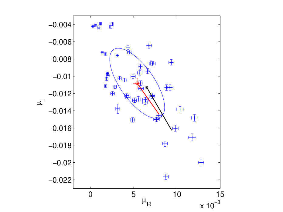
In Fig. 3 we display simulations for the mean displacement in the presence of an oscillating force on the tagged particle , for HT systems. Due to the non-universality of HT systems each realization of friction constants gives a different amplitude and phase for the oscillations around the mean position. The mean value as obtained with the average mobility () from Eqs. (18) and (19) shows satisfactory agreement with the simulations. Note the phase shift, between the applied force and the induced response in terms of the mean position. The mobility as extracted from simulations is a complex quantity with real part and imaginary part . The theoretical prediction for the mean of and are obtained from Eqs. (18) and (19) by setting and making a Wick rotation . To assess the variability around the mean mobility Fig. 4 displays a scatter plot of complex valued mobilities , , as extracted from simulations of different sets of frictions by
| (23) |
where are deviations from the average position for friction constant set , the runs over equally spaced times within one period of the force and represents an average over different periods within one set of friction constants. The average squared mobility estimated over the 50 different sets of frictions is , in satisfactory agreement with the corresponding analytic result obtained from Eqs. (18) and (19) with and .
VI Conclusion
Exactly solvable many-body models have over the years served all fields of physics, chemistry and biological sciences. The present manuscript provides important insights into the combined effects of heterogeneity and particle-particle interactions on the dynamics in stochastic processes. In particular, we provided an asymptotically exact analytic expression for the probability density of mobility in a single-file system, and for harmonically coupled beads, with different frictions constants. Our study paves the way for force response studies of other complex heterogeneous many-body systems.
We hope that the type of system introduced here will find experimental realizations for transport processes where heterogeneity is prominent - examples include, motion of flourescently labeled proteins on DNA molecules and other macromolecules, or diffusion of dissimilar particles in nanochannels.
VII Acknowledgements
T.A. acknowledges funding from the Knut & Alice Wallenberg Foundation and the Swedish Research Council (grant no. 2009-2924). Computer time was provided by the Danish Center for Scientific Computing.
Appendix A Asymptotic solution of Eq. (8)
Let us consider the expression for the distribution , Eq. (8) in the main text, for the case of long times (). In this limit Eq. (8) can be solved following the approach in the appendix of Ref. [29]. However, as this derivation is lengthy we here provide a simpler as well as more general version of the derivation. Following Ref. [29] we write
| (24) |
with the -dependent scaling function chosen to be positive and satisfying and as . Taking the Mellin-transform [] of Eq. (8) with respect to and substituting the integration variable with we get:
| (25) |
which is the starting point of our simplified derivation.
A.1 LT systems
Let us first consider light-tailed (LT) systems. For these we expand the right-hand-side of Eq. (25) to first subleading order in and . Also making use of the definition of a Mellin-transform we get that the right-hand side equals . Eq. (25) then becomes
| (26) |
We obtain a non-trivial solution for by choosing
| (27) |
where is the mean friction constant. The solution to Eq. (26) with (normalization condition) is simply which when Mellin-inverted gives
| (28) |
in agreement with [29].
A.2 HT systems
For heavy-tailed (HT) systems the analysis is slightly more involved. First we integrate Eq. (25) by parts, introducing the cumulative distribution , to find with
| (29) | ||||
| (30) |
Since for small we have . Restricting to the lower boundary term above vanishes. At the opposite boundary we have and thus we get
| (31) |
For , if we set and let we have and find to leading order in and :
| (32) |
Similarly we expand , but here we include the subleading term in
| (33) |
From Eqs. (32) and (33) we see that a way to obtain a non-trivial equation for in the limit is to choose
| (34) |
with . With this choice we find that satisfies
| (35) |
which has the solution (with )
| (36) |
in agreement with [29].
Appendix B The covariance matrix
Writing the mobility in Fourier space according to (with and real)
| (37) |
we can define a covariance matrix for the real and imaginary deviations
| (38) |
From simulation data with estimates , , of mobility from different sets of friction coefficients we estimate the average as . For the deviations we estimate the components of by
| (39) |
where and are either of or . The ellipse in Fig. 3 has been drawn with its center on , and with the major and minor radii equal to the square roots of the eigenvalues of the estimated . The corresponding axes points along the eigenvectors.
The analytic result for the second moment about the mean: allows us to extract two results regarding the covariance matrix . One regards its eigenvalues
| (40) |
The difference of these can be found from the analytic calculation of the moments as
| (41) |
Note that Eq. (41) implies that . We can also extract the eigenvectors. To see this first note that the asymptotic result for the th moment tells us that , where and , i.e., the phase of the second moment is twice that of the first moment. Using this we find that the eigenvector corresponding to is:
Thus, for the ellipse plotted in Fig. 3 of the main text we find that the major axis should point along the line to the origin. The black line in Fig. 3 drawn from the asterisk has length and points along as obtained from the analytic results.
References
- [1] R. Kubo, Science 233, 330 (1986).
- [2] U.M.B. Marconi, A. Puglisi, L. Rondini, A. Vulpiani, Phys. Rep. 461, 111 (2008).
- [3] C. Bustamante, Y.R. Chemla. N.R. Forde and D. Izhaky, Ann. Rev. Biochem. 73, 705 (2004).
- [4] C. Jarzynski, Phys. Rev. Lett. 78, 2690 (1997).
- [5] M. Gorissen, Alexandre Lazarescu, K. Mallick and C. Vanderzande, Phys. Rev. Lett. 109, 170601 (2012).
- [6] T. E. Harris, J. Appl. Prob. 2(2), 323 (1965).
- [7] M. Kollmann, Phys. Rev. Lett. 90, 180602 (2003).
- [8] F. Marchesoni and A. Taloni, Phys. Rev. Lett. 97, 106101 (2006).
- [9] E. Barkai and R. Silbey, Phys. Rev. Lett. 102, 050602 (2009).
- [10] C. Aslangul, J. Phys. A 33, 851 (2000).
- [11] A. Brzank and G.M. Schütz, J. Stat. Mech: Theory and Experiment P08028 (2007).
- [12] P. Goncalves and M. D. Jara, J. Stat. Phys. 132, 1135 (2008).
- [13] M. Jara, e-print: arXiv:0901.0229.
- [14] T. Ambjörnsson, L. Lizana, M.A. Lomholt and R.J. Silbey, J. Chem. Phys. 129, 185106 (2008).
- [15] O. Flomenbom, Phys. Rev. E 82, 031126 (2010).
- [16] M.A. Lomholt, L. Lizana and T. Ambjörnsson, J. Chem. Phys. 134, 045101 (2011).
- [17] V. Kukla, J. Kornatowski, D. Demuth, I. Girnus, H. Pfeifer, L. Rees, S. Schunk, K. Unger, and J. Kärger, Science 272, 702 (1996).
- [18] T. Meersmann, J.W. Logan, R. Simonutti, S. Caldarelli, A. Comotti, P. Sozzani, L.G. Kaiser and A. Pines, J. Phys. Chem. A 104, 11665 (2000).
- [19] K. Hahn, J. Kärger, and V. Kukla, Phys. Rev. Lett. 76, 2762 (1996).
- [20] Q. H. Wei, C. Bechinger, P. Leiderer, Science 287, 625 (2000).
- [21] V. Gupta, S.S. Nivarthi, A.V. McCormick, H. Ted Davis, Chem. Phys. Lett. 247, 596 (1995).
- [22] A. L. Hodgkin and R. D. Keynes, J. Physiol. (London) 128, 61 (1955).
- [23] K.C. Vermeulen, G.J. Stienen, C.F. Schmid, J Muscle Res Cell Motil. 23 71 (2002).
- [24] F. Berger, C. Keller, S. Klumpp, and R. Lipowsky, Phys. Rev. Lett. 108, 208101 (2012).
- [25] G.-W. Li, O.G. Berg and J. Elf, Nature Phys. 5, 294 (2009).
- [26] R. Kubo, Rep. Prog. Phys. 29, 255 (1966).
- [27] L. Lizana, T. Ambjörnsson, A. Taloni, E. Barkai, M. A. Lomholt, Phys. Rev. E 81, 051118 (2010).
- [28] The analysis performed here is similar to the one in appendix A of Ref. [16] (in Laplace-space rather than in the Fourier domain). The relation between our ’s and the quantities in Ref. [16] is: .
- [29] J. Bernasconi, W.R. Wyss and W. Wyss, Z. Physik B 37, 175 (1980).
- [30] S. Alexander, J. Bernasconi, and W. R. Schneider, Rev. Mod. Phys. 53, 175 (1981).
- [31] F. Oberhettinger, Tables of Mellin Transforms (Springer) New York (1974).
- [32] Milton Abramowitz and Irene A. Stegun, Handbook of Mathematical Functions with Formulas, Graphs, and Mathematical Tables, (Dover, New York, 1964).
- [33] A.M. Mathai, R.K. Saxena and H.J Haubold, The H-Function: Theory and Applications (Springer) 2010.