跳到论文正文
W Papers独立论文阅读器 arXiv:1402.4493 论文正文 计算阅读时间 · 0%
引用这篇论文根据当前论文元数据生成,正式投稿前建议核对。


License: arXiv.org perpetual non-exclusive license
arXiv:1402.4493v2 [math-ph] 13 May 2014

Arctic curves of the octahedron equation

Philippe Di Francesco Address: Department of Mathematics, University of Illinois at Urbana-Champaign, MC-382, 1409 W Green St., Urbana, IL 61801, U.S.A. e-mail: philippe@illinois.edu and Rodrigo Soto-Garrido Address: Department of Physics, University of Illinois at Urbana-Champaign, 1110 W. Green St., Urbana, IL 61801, U.S.A. e-mail: sotogar1@illinois.edu.
Date: August 24, 2026
Abstract.

We study the octahedron relation (also known as the A∞A_{\infty} TT-system), obeyed in particular by the partition function for dimer coverings of the Aztec Diamond graph. For a suitable class of doubly periodic initial conditions, we find exact solutions with a particularly simple factorized form. For these, we show that the density function that measures the average dimer occupation of a face of the Aztec graph, obeys a system of linear recursion relations with periodic coefficients. This allows us to explore the thermodynamic limit of the corresponding dimer models and to derive exact “arctic” curves separating the various phases of the system.

August 24, 2026

1. Introduction

The octahedron recurrence is a system of non-linear equations describing the evolution of a quantity Ti,j,kT_{i,j,k}, i,j,k∈ℤi,j,k\in{\mathbb{Z}} corresponding to discrete space (i,j)(i,j) and time kk. This equation first arose in the context of integrable quantum spin chains with a Lie group symmetry [33, 34], and is obeyed by the corresponding quantum transfer matrices. In this language, the octahedron equation corresponds to the so-called TT-system (for A∞A_{\infty}). In this formulation, the indices i,k,ji,k,j respectively stand for representation indices, and a discrete spectral parameter. The AA-type TT-systems have remarkable properties, depending on the choice of boundary conditions, such as discrete integrability [15], and periodicity properties [24, 17] as well as the positive Laurent property (solutions are Laurent polynomials of the initial data with non-negative integer coefficients) in relation to cluster algebras [11].

This equation or some restrictions thereof appear to be central in a number of combinatorial constructs, such as the Desnanot-Jacobi relation between minors of a given matrix and the Dodgson condensation of determinants [18], the lambda-determinant and alternating sign matrices [6, 39, 12], the puzzles for computing Littlewood-Richardson coefficients [32], various generalizations of Coxeter-Conway frieze patterns [10, 2, 4], and cluster algebra [14] to name a few.

A great progress in understanding the combinatorics of the octahedron equation was due to Speyer [41], who worked out the general solution in terms of a dimer model on a graph, also equivalent to the domino tiling problem of the Aztec diamond [19]. This establishes the connection between a general set of solutions of the octahedron equation with given initial data, and the partition functions of statistical lattice models of dimers, whose local Boltzmann weights are defined in terms of these data. This was recently extended to more general initial conditions, giving rise to dimer models on specific graphs [13]. Note also that a large class of dimer models on periodic graphs was recently shown to have both integrable and cluster algebra structures as well [23]. Finally, the study of the so-called pentagram map, an integrable dynamical system on polygons of projective plane displayed intriguing connections [22] with solutions of the octahedron equation with special periodic initial conditions. An analogous connection exists for the generalization to higher pentagram maps [21, 17, 28].

Dimer models were the subject of a lot of attention, starting with the so-called arctic circle theorem for the domino tilings of large Aztec diamonds [26], and later culminating in the global understanding of the arctic curve phenomenon in the continuum limit [29] [30], where the phase diagram of the model was shown to exhibit separations between frozen, disordered, and liquid phases. Analogous phenomena were observed for groves [35], for the double-dimer model connected to the hexahedron recurrence [31], for random walks [1], for square Young tableaux [40], and for the six-vertex model [9].

In the present paper, we revisit the case of domino tilings/dimer coverings of the Aztec diamond, from the point of view of Speyer’s general solution of the octahedron relation. We construct explicit exact solutions of the octahedron equation for an infinite class of initial data with special periodicity conditions. These in turn are partition functions for dimer models with periodic weights. For these solutions, we show that a certain local density function, that measures the average dimer occupation of a face of the Aztec graph, obeys a system of linear recursion relations with periodic coefficients. This allows to compute the density generating function explicitly in the form of a rational fraction. Following [36, 37, 38, 31], the study of the denominator of this function allows to explore the singularity structure of the dimer models in the thermodynamic limit of large size, and to confirm their phase structure, displaying frozen, disordered and facet-like phases separated by generalized “arctic” curves.

The paper is organized as follows.

In Section 2, we recall facts on the A∞A_{\infty} TT-system/octahedron equation and its initial conditions, as well as its solution as a dimer partition function on the Aztec graph. As a preparatory exercise, we compute the density generating function for the uniform initial data and show how to extract the arctic circle form the explicit solution.

In Section 3, we study in detail 2×22\times 2 periodic initial data, for which the TT-system is wrapped on the torus generated by (2,0)(2,0) and (0,2)(0,2) in ℤ2{\mathbb{Z}}^{2}. The density generating function is found to solve a linear 4×44\times 4 system, whose explicit solution displays two disconnected pieces of “arctic” curve, separating the dimer configurations in the thermodynamic limit into three phases: (i) four frozen corners with a single dominant configuration induced by the geometry of corners; (ii) a disordered “temperate region” analog to the inside of the arctic circle, and (iii) a new “facet”-like central phase, where the configurations are pinned to the sub-lattice corresponding to the faces with the smallest Boltzmann weight.

Section 4 is devoted to the class of so-called mm-toroidal boundary conditions. We first construct the explicit solution to the TT-system, and then show that it leads to linear systems for the density function with triply periodic coefficients in ℤ3{\mathbb{Z}}^{3}. As a result, the density generating function is shown to satisfy a 4​m×4​m4m\times 4m linear system, whose determinant captures the information on the generalized arctic curves that separate different phases. For this model, we find generically the same phases: (i) frozen corners; (ii) disordered region; (iii) in general m−1m-1 facets whose position and size vary with the initial data.

We gather a few concluding remarks in Section 5.

Acknowledgments. We thank E. Fradkin, M. Gekhtman, R. Kedem, R. Kenyon and G. Musiker for discussions. We thank the referees for a very thorough reading of the manuscript, and many useful remarks. P. D. F. thanks the Simons Center for Geometry and Physics for hospitality during the semester “Conformal Geometry” in the early stages of this work. P. D. F. is supported by the NSF grant DMS 13-01636 and the Morris and Gertrude Fine endowment. R. S. G. is supported by the NSF grant DMR-1064319 and the DOE grant DE-FG02-07ER46453 at the University of Illinois.

2. T-system, dimers and arctic curve

2.1. The A∞A_{\infty} TT-system.

The unrestricted A∞A_{\infty} TT-system (from now on we will drop the A∞A_{\infty} label), also known as the octahedron recurrence, is given by the following difference equation (for a detailed review of the TT-system see [34]):

(2.1) Ti,j,k+1​Ti,j,k−1=Ti+1,j,k​Ti−1,j,k+Ti,j+1,k​Ti,j−1,kT_{i,j,k+1}T_{i,j,k-1}=T_{i+1,j,k}T_{i-1,j,k}+T_{i,j+1,k}T_{i,j-1,k}

where i,j,k∈ℤi,j,k\in{\mathbb{Z}} and Ti,j,k∈ℝT_{i,j,k}\in{\mathbb{R}}. Notice that the system conserves parity i+j+k=0,1i+j+k=0,1 mod 2. Let us fix it to 11 throughout the paper. One way to think about the TT-system is to consider i,ji,j as labeling points on the square lattice and kk as a discrete time (as the vertical axis of a cubic lattice). In this sense the TT-system (2.1) describes the evolution in time of a given initial data (see Ref. [13]). In this paper we will work with a flat initial data, meaning that the value of the TT variables is specified on the (i,j,0)(i,j,0) and (i,j,1)(i,j,1) planes, namely we fix:

(2.2) Ti,j,i+j+1​mod​ 2=ti,j(i,j∈ℤ)T_{i,j,i+j+1\,{\rm mod}\,2}=t_{i,j}\qquad(i,j\in{\mathbb{Z}})

In this paper, we consider the solution Ti,j,kT_{i,j,k} to the TT-system (2.1) subject to various restrictions of the initial condition (2.2). These will be simply the result of imposing extra periodicity conditions on the initial data ti,jt_{i,j}, the simplest of which being the uniform case when all ti,j=1t_{i,j}=1.

2.2. Dimer formulation

Refer to caption
Figure 1. A typical Aztec diamond graph 𝒜i,j,k{\mathcal{A}_{i,j,k}} for k=4k=4 (a) with its face labeling, and a sample dimer configuration on 𝒜i,j,k{\mathcal{A}_{i,j,k}} (b). We have shaded the three types of faces: inner, corner, end, respectively adjacent to 4,2,1 edges of 𝒜i,j,k{\mathcal{A}}_{i,j,k}.

The solution Ti,j,kT_{i,j,k}, for i+j+k=1i+j+k=1 mod 2, i,j∈ℤi,j\in{\mathbb{Z}}, k≥0k\geq 0, of the A∞A_{\infty} TT-system (2.1) with initial data (2.2) was identified as the partition function for domino tilings of the Aztec diamond, or dually to the dimer coverings of the Aztec diamond graph 𝒜i,j,k{\mathcal{A}}_{i,j,k} [41, 13]. The graph 𝒜i,j,k{\mathcal{A}}_{i,j,k} has vertices at points of the lattice ℤ2{\mathbb{Z}}^{2}. Let us label the faces of ℤ2{\mathbb{Z}}^{2} by the coordinate (i,j)(i,j) of their lower left corner vertex. Then 𝒜i,j,k{\mathcal{A}}_{i,j,k} has faces (a,b)(a,b) such that |a−i|+|b−j|≤k−1|a-i|+|b-j|\leq k-1. Each such face receives the label ta,bt_{a,b}, the initial data assignment of the TT-system. The edges of the graph are inherited from those of the underlying square lattice, however the boundary faces have only one or two adjacent edges depending on whether they are corner faces or end faces (see Fig. 1 for an illustration). The vertices of 𝒜i,j,k{\mathcal{A}}_{i,j,k} are naturally bicolored black/white, according to the parity of i+j=0/1i+j=0/1 mod 2.

Definition 2.1.

The dimer model on 𝒜i,j,k{\mathcal{A}}_{i,j,k} is defined as follows. The configurations of the model are matchings of pairs of vertices connected via an edge (dimers) such that any vertex of 𝒜i,j,k{\mathcal{A}}_{i,j,k} belongs to exactly one dimer. Each configuration is weighted by a product over all faces (a,b)(a,b) of 𝒜i,j,k{\mathcal{A}}_{i,j,k} of local weights wa,bw_{a,b}. For any face (a,b)(a,b) (including boundary faces) the weight is

wa,b=(ta,b)1−Da,bw_{a,b}=(t_{a,b})^{1-D_{a,b}}

where Da,b∈{0,1,2}D_{a,b}\in\{0,1,2\} is the total number of dimers occupying the edges of the square face. The partition function of the model is

Zi,j,k=∑dimerconfigurations∏faces⁡(a,b)wa,bZ_{i,j,k}=\sum_{{\rm dimer}\atop{\rm configurations}}\prod_{{\rm faces}\ (a,b)}w_{a,b}

The analysis of the present paper is based on the following main result:

Theorem 2.2.

[41, 13] The solution Ti,j,kT_{i,j,k}, for i+j+k=1i+j+k=1 mod 2, i,j∈ℤi,j\in{\mathbb{Z}}, k≥0k\geq 0, of the A∞A_{\infty} TT-system (2.1) with initial data (2.2) is the partition function of the dimer model on 𝒜i,j,k{\mathcal{A}}_{i,j,k}, namely

Ti,j,k=Zi,j,kT_{i,j,k}=Z_{i,j,k}

2.2.1. Density

Consider the solution Ti,j,kT_{i,j,k} to the TT-system with initial data (2.2). If we think of Ti,j,kT_{i,j,k} as a partition function, then the derivative tϵ,η​∂tϵ,ηLog​Ti,j,kt_{\epsilon,\eta}\partial_{t_{\epsilon,\eta}}{\rm Log}\,T_{i,j,k} corresponds to some susceptibility or density, where tϵ,ηt_{\epsilon,\eta} acts as a source, here a magnetic field attached to dimers around the (ϵ,η)(\epsilon,\eta) face. More precisely, we have

tϵ,η​∂tϵ,ηLog​Ti,j,k=⟨1−Dϵ,η⟩,t_{\epsilon,\eta}\partial_{t_{\epsilon,\eta}}{\rm Log}\,T_{i,j,k}=\langle 1-D_{\epsilon,\eta}\rangle\ ,

the statistical average of 1−1- the number of dimers surrounding the face (ϵ,η)(\epsilon,\eta) within the set of dimer configurations on 𝒜i,j,k{\mathcal{A}}_{i,j,k}. Assume we further restrict the initial values to ta,b=ta,b∗t_{a,b}=t_{a,b}^{*}, a,b∈ℤa,b\in{\mathbb{Z}}.

Definition 2.3.

We define the density function ρi,j,k(ϵ,η)\rho_{i,j,k}^{(\epsilon,\eta)} as:

(2.3) ρi,j,k(ϵ,η)=tϵ,η​∂tϵ,ηLog​Ti,j,k|ta,b=ta,b∗\rho_{i,j,k}^{(\epsilon,\eta)}=t_{\epsilon,\eta}\left.\partial_{t_{\epsilon,\eta}}{\rm Log}\,T_{i,j,k}\right|_{t_{a,b}=t_{a,b}^{*}}

We can easily derive a linear recurrence relation for ρi,j,k(ϵ,η)\rho_{i,j,k}^{(\epsilon,\eta)} by taking the derivative with respect to tϵ,ηt_{\epsilon,\eta} of the TT-system relation (2.1). After some straightforward algebra we have:

(2.4) ρi,j,k+1(ϵ,η)+ρi,j,k−1(ϵ,η)=Li,j,k​(ρi+1,j,k(ϵ,η)+ρi−1,j,k(ϵ,η))+Ri,j,k​(ρi,j+1,k(ϵ,η)+ρi,j−1,k(ϵ,η))\rho_{i,j,k+1}^{(\epsilon,\eta)}+\rho_{i,j,k-1}^{(\epsilon,\eta)}=L_{i,j,k}(\rho_{i+1,j,k}^{(\epsilon,\eta)}+\rho_{i-1,j,k}^{(\epsilon,\eta)})+R_{i,j,k}(\rho_{i,j+1,k}^{(\epsilon,\eta)}+\rho_{i,j-1,k}^{(\epsilon,\eta)})

where we used the notation:

(2.5) Li,j,k=Ti+1,j,k​Ti−1,j,kTi,j,k+1​Ti,j,k−1andRi,j,k=1−Li,j,k=Ti,j+1,k​Ti,j−1,kTi,j,k+1​Ti,j,k−1L_{i,j,k}=\displaystyle\frac{T_{i+1,j,k}T_{i-1,j,k}}{T_{i,j,k+1}T_{i,j,k-1}}\qquad{\rm and}\qquad R_{i,j,k}=1-L_{i,j,k}=\displaystyle\frac{T_{i,j+1,k}T_{i,j-1,k}}{T_{i,j,k+1}T_{i,j,k-1}}

where Ti,j,kT_{i,j,k} are evaluated at ta,b=ta,b∗t_{a,b}=t_{a,b}^{*} for all a,b∈ℤa,b\in{\mathbb{Z}}. The recurrence relation is supplemented with the following initial data. Define φ=(ϵ+η+1​mod​ 2)\varphi=(\epsilon+\eta+1\ {\rm mod}\ 2). Then:

(2.6) ρi,j,φ(ϵ,η)=δi,ϵδj,ηρi,j,1−φ(ϵ,η)=0(i,j∈ℤ;i+j+ϵ+η=0mod 2)\rho_{i,j,\varphi}^{(\epsilon,\eta)}=\delta_{i,\epsilon}\delta_{j,\eta}\qquad\rho_{i,j,1-\varphi}^{(\epsilon,\eta)}=0\qquad(i,j\in{\mathbb{Z}};i+j+\epsilon+\eta=0\,{\rm mod}\,2)

Notice that in order to solve the recurrence relation for the density we need to know Li,j,kL_{i,j,k} and Ri,j,kR_{i,j,k} appearing in (2.4). As we shall see below, the density ρi,j,k(ϵ,η)\rho_{i,j,k}^{(\epsilon,\eta)} is the variable that we will use to explore the behavior of the dimer model for large kk.

2.3. Arctic curve: the uniform case

We start with the recurrence relation (2.4) for the uniform initial data:

(2.7) ti,j∗=1(i,j∈ℤ)t_{i,j}^{*}=1\qquad(i,j\in{\mathbb{Z}})

In this case the solution for the T-system is simply given by Ti,j,k=2k⁡(k−1)/2T_{i,j,k}=2^{k(k-1)/2}: this coincides with the partition function of uniform domino tilings of an Aztec diamond of size kk [19]. The two ratios Li,j,kL_{i,j,k}, Ri,j,kR_{i,j,k} appearing in eq. (2.4) are equal to 1/21/2.

To this uniform initial data we add up a source on the face (ϵ,η)=(0,0)(\epsilon,\eta)=(0,0) or (0,1)(0,1), namely consider the densities ρi,j,k(0,0)\rho_{i,j,k}^{(0,0)}, ρi,j,k(0,1)\rho_{i,j,k}^{(0,1)}. Both densities obey the following recurrence relation:

(2.8) ρi,j,k+1+ρi,j,k−1=12​(ρi+1,j,k+ρi−1,j,k+ρi,j+1,k+ρi,j−1,k)(i,j∈ℤ,k≥1)\rho_{i,j,k+1}+\rho_{i,j,k-1}=\frac{1}{2}(\rho_{i+1,j,k}+\rho_{i-1,j,k}+\rho_{i,j+1,k}+\rho_{i,j-1,k})\qquad(i,j\in{\mathbb{Z}};k\geq 1)

with initial data ρi,j,0(0,0)=0\rho_{i,j,0}^{(0,0)}=0 and ρi,j,1(0,0)=δi,0​δj,0\rho_{i,j,1}^{(0,0)}=\delta_{i,0}\delta_{j,0}, while ρi,j,1(0,1)=0\rho_{i,j,1}^{(0,1)}=0 and ρi,j,0(0,1)=δi,0​δj,0\rho_{i,j,0}^{(0,1)}=\delta_{i,0}\delta_{j,0}. Extending the validity of (2.8) to k=0k=0 allows to define

(2.9) ρi,j,−1(0,0)=−δi,0​δj,0\rho_{i,j,-1}^{(0,0)}=-\delta_{i,0}\delta_{j,0}

and

(2.10) ρi,j,−1(0,1)=12​(δi,−1+δi,1)​δj,0+12​(δj,−1+δj,1)​δi,0\rho_{i,j,-1}^{(0,1)}=\frac{1}{2}(\delta_{i,-1}+\delta_{i,1})\delta_{j,0}+\frac{1}{2}(\delta_{j,-1}+\delta_{j,1})\delta_{i,0}

For (ϵ,η)=(0,0)(\epsilon,\eta)=(0,0) or (0,1)(0,1), we define generating functions ρ(ϵ,η)​(x,y,z)\rho^{(\epsilon,\eta)}(x,y,z) as:

(2.11) ρ(ϵ,η)​(x,y,z)=∑i,j∈ℤ,k≥0ρi,j,k(ϵ,η)​xi​yj​zk\rho^{(\epsilon,\eta)}(x,y,z)=\sum_{i,j\in{\mathbb{Z}},k\geq 0}\rho_{i,j,k}^{(\epsilon,\eta)}\,x^{i}\,y^{j}\,z^{k}

Multiplying both sides of (2.8) by xi​yj​zkx^{i}y^{j}z^{k} and then summing over i,j∈ℤ,k≥0i,j\in{\mathbb{Z}},k\geq 0 we get:

∑i,j∈ℤ,k≥0(ρi,j,k+1+ρi,j,k−1)​xi​yj​zk=12​∑i,j∈ℤ,k≥0(ρi+1,j,k+ρi−1,j,k+ρi,j+1,k+ρi,j−1,k)​xi​yj​zk\sum_{i,j\in{\mathbb{Z}},k\geq 0}(\rho_{i,j,k+1}+\rho_{i,j,k-1})x^{i}y^{j}z^{k}=\frac{1}{2}\sum_{i,j\in{\mathbb{Z}},k\geq 0}(\rho_{i+1,j,k}+\rho_{i-1,j,k}+\rho_{i,j+1,k}+\rho_{i,j-1,k})x^{i}y^{j}z^{k}

for both density functions. Substituting the values of ρi,j,−1\rho_{i,j,-1} from (2.9-2.10), we get:

(z−1+z)​ρ(0,0)​(x,y,z)\displaystyle(z^{-1}+z)\rho^{(0,0)}(x,y,z) =\displaystyle= 12​(x−1+x+y−1+y)​ρ(0,0)​(x,y,z)+1\displaystyle\frac{1}{2}(x^{-1}+x+y^{-1}+y)\rho^{(0,0)}(x,y,z)+1
(z−1+z)​ρ(0,1)​(x,y,z)\displaystyle(z^{-1}+z)\rho^{(0,1)}(x,y,z) =\displaystyle= 12​(x−1+x+y−1+y)​ρ(0,1)​(x,y,z)+z−1−12​(x−1+x+y−1+y)\displaystyle\frac{1}{2}(x^{-1}+x+y^{-1}+y)\rho^{(0,1)}(x,y,z)+z^{-1}-\frac{1}{2}(x^{-1}+x+y^{-1}+y)

So the density generating functions for the uniform initial data are given by:

ρ(0,0)​(x,y,z)\displaystyle\rho^{(0,0)}(x,y,z) =\displaystyle= z1+z2−z2​(x−1+x+y−1+y)\displaystyle\frac{z}{1+z^{2}-\frac{z}{2}(x^{-1}+x+y^{-1}+y)}
(2.12) ρ(0,1)​(x,y,z)\displaystyle\rho^{(0,1)}(x,y,z) =\displaystyle= 1−z2​(x−1+x+y−1+y)1+z2−z2​(x−1+x+y−1+y)\displaystyle\frac{1-\frac{z}{2}(x^{-1}+x+y^{-1}+y)}{1+z^{2}-\frac{z}{2}(x^{-1}+x+y^{-1}+y)}
=\displaystyle= 1−z​ρ(0,0)​(x,y,z)​(x,y,z)\displaystyle 1-z\,\rho^{(0,0)}(x,y,z)(x,y,z)

Recall that ρi,j,k(0,0)\rho^{(0,0)}_{i,j,k}, i+j+k=1i+j+k=1 mod 2, is the average ⟨1−D0,0⟩i,j,k\langle 1-D_{0,0}\rangle_{i,j,k} in the dimer model on 𝒜i,j,k{\mathcal{A}}_{i,j,k}. It is the same as the average ⟨1−D−i,−j⟩0,0,k\langle 1-D_{-i,-j}\rangle_{0,0,k} (for i+ji+j even) in the dimer model on 𝒜0,0,k{\mathcal{A}}_{0,0,k} when kk is odd and as ⟨1−D−i,−j+1⟩0,1,k\langle 1-D_{-i,-j+1}\rangle_{0,1,k} (for i+ji+j odd) in the dimer model on 𝒜0,1,k{\mathcal{A}}_{0,1,k} when kk is even. Therefore the generating function for the averages ⟨1−Di,j⟩0,0,2​k−1\langle 1-D_{i,j}\rangle_{0,0,2k-1} on the even faces (with i+j=0i+j=0 mod 2) of the dimer model on A0,0,2​k−1A_{0,0,2k-1} reads:

∑i,j∈ℤi+j​even⟨1−Di,j⟩0,0,2​k−1​xi​yj=ρ(0,0)​(x−1,y−1,z)|z2​k−1=ρ(0,0)​(x,y,z)|z2​k−1\sum_{i,j\in{\mathbb{Z}}\atop i+j\ {\rm even}}\langle 1-D_{i,j}\rangle_{0,0,2k-1}\,x^{i}\,y^{j}=\rho^{(0,0)}(x^{-1},y^{-1},z)|_{z^{2k-1}}=\rho^{(0,0)}(x,y,z)|_{z^{2k-1}}

by use of the obvious symmetries x↔x−1x\leftrightarrow x^{-1} and y↔y−1y\leftrightarrow y^{-1} of ρ(0,0)\rho^{(0,0)} (2.12), and where the notation f|zmf|_{z^{m}} stands for the coefficient of zmz^{m} in the power expansion of ff as a series of zz. Similarly, the generating function for the averages ⟨1−Di,j⟩0,1,2​k\langle 1-D_{i,j}\rangle_{0,1,2k} on the even faces of the dimer model on A0,1,2​kA_{0,1,2k} reads:

∑i,j∈ℤi+j​even⟨1−Di,j⟩0,1,2​k​xi​yj=y​ρ(0,0)​(x−1,y−1,z)|z2​k−1=y​ρ(0,0)​(x,y,z)|z2​k\sum_{i,j\in{\mathbb{Z}}\atop i+j\ {\rm even}}\langle 1-D_{i,j}\rangle_{0,1,2k}\,x^{i}\,y^{j}=y\,\rho^{(0,0)}(x^{-1},y^{-1},z)|_{z^{2k-1}}=y\,\rho^{(0,0)}(x,y,z)|_{z^{2k}}

We have similar expressions for the averages on odd faces, involving ρ(0,1)\rho^{(0,1)}.

Refer to caption
Figure 2. Arctic circle for the trivial initial data. The corners are frozen and the center is disordered.

The singularities of these two expressions are determined by the denominator of ρ(0,0)​(x,y,z)\rho^{(0,0)}(x,y,z) given by (2.12).

We wish to explore the behavior of the coefficients ρi,j,k(0,0)\rho^{(0,0)}_{i,j,k} for large i,j,ki,j,k and ik=u\frac{i}{k}=u, jk=v\frac{j}{k}=v finite. Following the general theory of singularities of multivariate series [36, 37, 38], the limit is singular along the planar dual curve to the homogeneous polynomial part of the denominator of the generating functions at the critical point x=y=z=1x=y=z=1. To compute this curve, we may blow up the singular point x=y=z=1x=y=z=1 by taking x→1−t​xx\rightarrow 1-tx, y→1−t​yy\rightarrow 1-ty and z→1+t⁡(u​x+v​y)z\rightarrow 1+t(ux+vy) and then expand the denominator in powers of tt. Up to order t2t^{2} we have:

z−1+z−12​(x−1+x+y−1+y)=t22​((2​u2−1)​x2+(2​v2−1)​y2+4​u​v​x​y)+O⁡(t3)z^{-1}+z-\frac{1}{2}(x^{-1}+x+y^{-1}+y)=\frac{t^{2}}{2}((2u^{2}-1)x^{2}+(2v^{2}-1)y^{2}+4uvxy)+O(t^{3})

Let us define H⁡(x,y)=(2​u2−1)​x2+(2​v2−1)​y2+4​u​v​x​yH(x,y)=(2u^{2}-1)x^{2}+(2v^{2}-1)y^{2}+4uvxy. The dual curve is obtained by imposing H⁡(x,y)=0H(x,y)=0 and ∂∂x​H​(x,y)=∂∂y​H​(x,y)=0\frac{\partial}{\partial x}H(x,y)=\frac{\partial}{\partial y}H(x,y)=0. However, here and in the following, H⁡(x,y)H(x,y) is always a homogeneous polynomial, henceforth (∂∂x+y​∂∂y)​H=m​H(\frac{\partial}{\partial x}+y\frac{\partial}{\partial y})H=mH, where mm is the total degree, m=2m=2 here. We may therefore simply impose H⁡(x,y)=0H(x,y)=0 and ∂∂x​H​(x,y)=0\frac{\partial}{\partial x}H(x,y)=0, and the last equation ∂∂y​H​(x,y)=0\frac{\partial}{\partial y}H(x,y)=0 is automatically satisfied. Eliminating xx and yy, we end up with the singularity locus:

(2.13) P⁡(u,v)=2​(u2+v2)−1=0P(u,v)=2(u^{2}+v^{2})-1=0

This defines the arctic circle (see Fig. 2). This is the circle inscribed into the square domain |u|+|v|=1|u|+|v|=1, which corresponds to the limiting domain of non-zero values of ρi,j,k\rho_{i,j,k} for k→∞k\to\infty while ik=u\frac{i}{k}=u, jk=v\frac{j}{k}=v.

3. Toroidal initial data I: the 2×\times2 case

Refer to caption

b b b b b b b b b b b b b b b b d d d d d d d d d d d d a a a a a a a a a c c c c c c c c c c c c j i (0,0)

Figure 3. Initial data with period 2 in directions i,ji,j. The white and black points corresponds to the planes k=0k=0 and k=1k=1 respectively.

In this section we will focus on a very specific initial data, which has period two in both ii and jj directions, namely:

ti+2,j=ti,jti,j+2=ti,jt_{i+2,j}=t_{i,j}\qquad t_{i,j+2}=t_{i,j}

More precisely, we set (see Fig. 3):

(3.1) ti,j={aif​i=0,j=0​mod​ 2bif​i=1,j=1​mod​ 2cif​i=0,j=1​mod​ 2dif​i=1,j=0​mod​ 2t_{i,j}=\left\{\begin{matrix}a&{\rm if}\,i=0,j=0\,{\rm mod}\,2\\ b&{\rm if}\,i=1,j=1\,{\rm mod}\,2\\ c&{\rm if}\,i=0,j=1\,{\rm mod}\,2\\ d&{\rm if}\,i=1,j=0\,{\rm mod}\,2\end{matrix}\right.

Remarkably, this particular initial data allows us to still find an exact and simple solution for the TT-system. At the same time it provides us with an illustrative example on how to compute the arctic curves for non-uniform initial data. We will see that the ratios Li,j,kL_{i,j,k} and Ri,j,kR_{i,j,k} appearing in (2.4) have a certain periodicity that allows to reduce the problem to a finite linear system of 4 equations (each for different values of the ratios).

3.1. Exact solution of the TT-system with 2×\times2 periodic initial data

The corresponding TT-system actually coincides with the so-called QQ-system for A1^\widehat{A_{1}}. The exact solution to this T-system with doubly periodic initial data is given by:

Lemma 3.1.
(3.2) Ti,j,k=(a2+b2c​d)⌊k2⌋​⌊k+12⌋​(c2+d2a​b)⌊k−12⌋​⌊k2⌋×{ti,j, if k=0,1,mod 4ti+1,j+1, if k=2,3,mod 4T_{i,j,k}=\left(\frac{a^{2}+b^{2}}{cd}\right)^{\left\lfloor\frac{k}{2}\right\rfloor\left\lfloor\frac{k+1}{2}\right\rfloor}\left(\frac{c^{2}+d^{2}}{ab}\right)^{\left\lfloor\frac{k-1}{2}\right\rfloor\left\lfloor\frac{k}{2}\right\rfloor}\times\begin{cases}t_{i,j}&,\text{ if }k=0,1,\ {\rm mod}\ 4\\ t_{i+1,j+1}&,\text{ if }k=2,3,\ {\rm mod}\ 4\end{cases}

for ti,jt_{i,j} as in (3.1).

Proof.

By direct substitution into the octahedron recurrence (2.1), and inspection of the cases k=0,1,2,3k=0,1,2,3 mod 4. ∎

3.2. Density: exact derivation

As explained before, we may consider various density functions ρi,j,k(ϵ,η)\rho^{(\epsilon,\eta)}_{i,j,k} that measure the average ⟨1−Dϵ,η⟩i,j,k\langle 1-D_{\epsilon,\eta}\rangle_{i,j,k} on the face (ϵ,η)(\epsilon,\eta) of the dimer model on 𝒜i,j,k{\mathcal{A}}_{i,j,k}. For odd kk this is equal to the average ⟨1−Dϵ−i,η−j⟩0,0,k\langle 1-D_{\epsilon-i,\eta-j}\rangle_{0,0,k} of the dimer model on 𝒜0,0,k{\mathcal{A}}_{0,0,k} (in which the central face is of aa type).

Let us consider only even faces of type aa or bb, namely ϵ=η=0\epsilon=\eta=0 or 11, and kk odd. Then the density ρ(0,0)​(x−1,y−1,z)|xeven​yeven\rho^{(0,0)}(x^{-1},y^{-1},z)|_{x^{\rm even}y^{\rm even}} generates ⟨1−Di,j⟩0,0,k\langle 1-D_{i,j}\rangle_{0,0,k} on aa-type faces with both i,ji,j even, while x​y​(ρ(1,1)​(x−1,y−1,z)|xeven​yeven)xy\left(\rho^{(1,1)}(x^{-1},y^{-1},z)|_{x^{\rm even}y^{\rm even}}\right) generates ⟨1−Di,j⟩0,0,k\langle 1-D_{i,j}\rangle_{0,0,k} on bb-type faces with both i,ji,j odd. By considering odd powers of x,yx,y instead, we have also access to averages of 1−Di,j1-D_{i,j} for 𝒜1,1,k{\mathcal{A}}_{1,1,k} (in which the central face is of bb type).

Now that we have a solution for the TT-system, we can directly compute the ratios in the recurrence relation for the density (2.4). We note that the ratio Li,j,kL_{i,j,k} is periodic (as well as Ri,j,kR_{i,j,k}, from the relation Li,j,k+Ri,j,k=1L_{i,j,k}+R_{i,j,k}=1). We have indeed an obvious periodicity on the constant kk planes. Defining e1=(2,0,0)e_{1}=(2,0,0) and e2=(0,2,0)e_{2}=(0,2,0), we have that L(i,j,k)=L(i,j,k)+m​e1+n​e2L_{(i,j,k)}=L_{(i,j,k)+me_{1}+ne_{2}} where m,n∈ℤm,n\in{\mathbb{Z}} (the same for Ri,j,kR_{i,j,k}). However, by using the exact solution (3.2), we find another less obvious periodicity in the direction e3=(1,1,2)e_{3}=(1,1,2) as well. This is summarized in the following:

Lemma 3.2.

The coefficients Li,j,k,Ri,j,kL_{i,j,k},R_{i,j,k} corresponding to the 2×22\times 2 periodic solution (3.2) of the TT-system have the following periodicity:

L(i,j,k)=L(i,j,k)+m​e1+n​e2+p​e3(m,n∈ℤ,p≥0).L_{(i,j,k)}=L_{(i,j,k)+me_{1}+ne_{2}+pe_{3}}\qquad(m,n\in{\mathbb{Z}},p\geq 0).

and similarly for Ri,j,k=1−Li,j,kR_{i,j,k}=1-L_{i,j,k}.

Proof.

By inspection. ∎

Let us first derive ρ(0,0)​(x,y,z)\rho^{(0,0)}(x,y,z). Define the following partial generating functions:

(3.3) ρ(i0,j0,k0)​(x,y,z)=∑m,n∈ℤ,p≥0ρ(i0,j0,k0)+m​e1+n​e2+p​e3(0,0)​xi0+2​m+p​yj0+2​n+p​zk0+2​p\rho^{(i_{0},j_{0},k_{0})}(x,y,z)=\sum_{m,n\in{\mathbb{Z}},p\geq 0}\rho^{(0,0)}_{(i_{0},j_{0},k_{0})+me_{1}+ne_{2}+pe_{3}}\,x^{i_{0}+2m+p}y^{j_{0}+2n+p}z^{k_{0}+2p}

where (i0,j0,k0)(i_{0},j_{0},k_{0}) are in the unit cell for the periodicities of Lemma 3.2, namely (i0,j0,k0)∈P={(0,0,1),(1,1,1),(1,0,0),(0,1,0)}(i_{0},j_{0},k_{0})\in P=\{(0,0,1),(1,1,1),(1,0,0),(0,1,0)\}. In terms of these the full density generating function is simply

ρ(0,0)​(x,y,z)=∑(i0,j0,k0)∈Pρ(i0,j0,k0)​(x,y,z)\rho^{(0,0)}(x,y,z)=\sum_{(i_{0},j_{0},k_{0})\in P}\rho^{(i_{0},j_{0},k_{0})}(x,y,z)

Using the recurrence relation for the density (2.4) and the initial conditions ρi,j,1(0,0)=δi,0​δj,0\rho^{(0,0)}_{i,j,1}=\delta_{i,0}\delta_{j,0}, ρi,j,0(0,0)=0\rho^{(0,0)}_{i,j,0}=0, we end up with the following linear system:

(3.4) (1z(x2+1)​(τ−1)x−(y2+1)​τyzz(y2+1)​(τ−1)y−(x2+1)​τx1z−(y2+1)​σy1zz(x2+1)​(σ−1)x−(x2+1)​σxz1z(y2+1)​(σ−1)y)​(ρ(0,0,1)​(x,y,z)ρ(0,1,0)​(x,y,z)ρ(1,0,0)​(x,y,z)ρ(1,1,1)​(x,y,z))=(1000)\left(\begin{array}[]{cccc}\frac{1}{z}&\frac{\left(x^{2}+1\right)(\tau-1)}{x}&-\frac{\left(y^{2}+1\right)\tau}{y}&z\\ z&\frac{\left(y^{2}+1\right)(\tau-1)}{y}&-\frac{\left(x^{2}+1\right)\tau}{x}&\frac{1}{z}\\ -\frac{\left(y^{2}+1\right)\sigma}{y}&\frac{1}{z}&z&\frac{\left(x^{2}+1\right)(\sigma-1)}{x}\\ -\frac{\left(x^{2}+1\right)\sigma}{x}&z&\frac{1}{z}&\frac{\left(y^{2}+1\right)(\sigma-1)}{y}\end{array}\right)\left(\begin{array}[]{c}\rho^{(0,0,1)}(x,y,z)\\ \rho^{(0,1,0)}(x,y,z)\\ \rho^{(1,0,0)}(x,y,z)\\ \rho^{(1,1,1)}(x,y,z)\end{array}\right)=\left(\begin{array}[]{c}1\\ 0\\ 0\\ 0\end{array}\right)

where we have used the parametrizations of weights:

σ=L1,0,1=a2a2+b2,τ=R0,0,0=c2c2+d2,\sigma=L_{1,0,1}=\frac{a^{2}}{a^{2}+b^{2}},\qquad\tau=R_{0,0,0}=\frac{c^{2}}{c^{2}+d^{2}}\,,

or equivalently:

a=b​σ1−σ,andc=d​τ1−τ.a=b\sqrt{\frac{\sigma}{1-\sigma}},\qquad{\rm and}\qquad c=d\sqrt{\frac{\tau}{1-\tau}}\,.

It is worth noticing that even though we started with 4 arbitrary values a,b,c,da,b,c,d in our initial data in the 2×22\times 2 torus, the corresponding system for the density only depends on 2 parameters, the ratios a/ba/b and c/dc/d. As we saw in the case of the uniform initial data, the arctic curve is determined by the zero locus of the denomiator of the density functions. Here, this denominator is given by the determinant of the above system of 4 equations. Defining

(3.5) α=16​σ​(1−σ)​τ​(1−τ)=16(ab+ba)2​(cd+dc)2\alpha=16\sigma(1-\sigma)\tau(1-\tau)=\frac{16}{\left(\frac{a}{b}+\frac{b}{a}\right)^{2}\left(\frac{c}{d}+\frac{d}{c}\right)^{2}}

then, up to a factor of x​y​zxyz, the determinant reads:

(3.6) D⁡(x,y,z)=α16​(x2−y2)2​(x2​y2−1)2​z4−x2​y2​(x​y−z2)​(y−x​z2)​(x−y​z2)​(1−x​y​z2)D(x,y,z)=\frac{\alpha}{16}(x^{2}-y^{2})^{2}(x^{2}y^{2}-1)^{2}z^{4}-x^{2}y^{2}\left(xy-z^{2}\right)\left(y-xz^{2}\right)\left(x-yz^{2}\right)\left(1-xyz^{2}\right)

The actual density ρ(0,0)​(x,y,z)\rho^{(0,0)}(x,y,z) however depends explicitly on σ,τ\sigma,\tau, not just on α\alpha. It has the form ρ(0,0)​(x,y,z)=Q(0,0)​(x,y,z)D⁡(x,y,z)\rho^{(0,0)}(x,y,z)=\frac{Q^{(0,0)}(x,y,z)}{D(x,y,z)}, with DD as in (3.6), and Q(0,0)Q^{(0,0)} the following polynomial of x,y,zx,y,z:

(3.7) Q(0,0)​(x,y,z)\displaystyle Q^{(0,0)}(x,y,z) =\displaystyle= xyz{(−x2y2(1−z2)(z(x(1−xyz2)+y(xy−z2))+xy(1−z4))\displaystyle xyz\left\{(-x^{2}y^{2}(1-z^{2})(z(x(1-xyz^{2})+y(xy-z^{2}))+xy(1-z^{4}))\right.
−x​y​(x−y)​(1−x​y)​z2​(x⁡(1−x​y​z2)+y⁡(x​y−z2))​σ+x2​y2​(x−y)​(1−x​y)​z​(1−z4)​τ\displaystyle-xy(x-y)(1-xy)z^{2}(x(1-xyz^{2})+y(xy-z^{2}))\sigma+x^{2}y^{2}(x-y)(1-xy)z(1-z^{4})\tau
+xy(x2−y2)(1−x2y2)z2(1−z2)στ−(x−y)(x2−y2)(1−xy)(1−x2y2)z3στ(1−τ)}\displaystyle\left.+xy(x^{2}-y^{2})(1-x^{2}y^{2})z^{2}(1-z^{2})\sigma\tau-(x-y)(x^{2}-y^{2})(1-xy)(1-x^{2}y^{2})z^{3}\sigma\tau(1-\tau)\right\}

Similarly, the density ρ(1,1)​(x,y,z)\rho^{(1,1)}(x,y,z) solves the same system (3.4), but with the r.h.s. replaced by (0,x​y,0,0)t(0,xy,0,0)^{t}, due to the initial conditions ρi,j,1(1,1)=δi,1​δj,1\rho^{(1,1)}_{i,j,1}=\delta_{i,1}\delta_{j,1} and ρi,j,0(1,1)=0\rho^{(1,1)}_{i,j,0}=0. Alternatively, ρ(1,1)/(x​y)\rho^{(1,1)}/(xy) is obtained by interchanging a↔ba\leftrightarrow b and c↔dc\leftrightarrow d in the expression for ρ(0,0)\rho^{(0,0)}, namely by performing the substitutions σ→1−σ\sigma\to 1-\sigma and τ→1−τ\tau\to 1-\tau. These produce a new numerator Q(1,1)Q^{(1,1)}, but leave the denominator D⁡(x,y,z)D(x,y,z) unchanged.

3.3. Arctic curve

Using the same procedure as for the uniform initial data, we expand the denominator D⁡(x,y,z)D(x,y,z) around the critical point x=y=z=1x=y=z=1. Taking x→1−t​xx\rightarrow 1-tx, y→1−t​yy\rightarrow 1-ty and z→1+t⁡(u​x+v​y)z\rightarrow 1+t(ux+vy), we find D⁡(1−t​x,1−t​y,1+t⁡(u​x+v​y))=t4​H​(x,y)+O⁡(t5)D(1-tx,1-ty,1+t(ux+vy))=t^{4}H(x,y)+O(t^{5}) at leading order in tt (which in this case turns out to be t4t^{4}). Imposing again H⁡(x,y)=0H(x,y)=0 and ∂∂x​H​(x,y)=0\frac{\partial}{\partial x}H(x,y)=0, we can eliminate xx and yy. We finally get the singularity curve Pα​(u,v)=0P_{\alpha}(u,v)=0, where:

(3.8) Pα​(u,v)=(1−α)3+16​α2​(u8+v8)+8​(4−5​α)​α​(u6+v6)+32​(α2+2​(2−α)2)​u4​v4+((4−α)2−24​α)​(1−α)​(u4+v4)+8​(6​α2−(4−α)2)​u2​v2​(u2+v2)+2​(48−(4−α)2)​(1−α)​u2​v2−2​(1−α)2​(4−α)​(u2+v2)+64​(2−α)​α​u2​v2​(u4+v4)\begin{split}P_{\alpha}(u,v)=&(1-\alpha)^{3}+16\alpha^{2}(u^{8}+v^{8})+8(4-5\alpha)\alpha(u^{6}+v^{6})+32\left(\alpha^{2}+2(2-\alpha)^{2}\right)u^{4}v^{4}\\ &+\left((4-\alpha)^{2}-24\alpha\right)(1-\alpha)\left(u^{4}+v^{4}\right)+8\left(6\alpha^{2}-(4-\alpha)^{2}\right)u^{2}v^{2}\left(u^{2}+v^{2}\right)\\ &+2\left(48-(4-\alpha)^{2}\right)(1-\alpha)u^{2}v^{2}-2(1-\alpha)^{2}(4-\alpha)(u^{2}+v^{2})+64(2-\alpha)\alpha u^{2}v^{2}(u^{4}+v^{4})\end{split}

Notice that this polynomial depends only on the single parameter α{\alpha} of (3.5). Let us examine a few limiting cases of interest.

Refer to caption → α 0 = α / 1 2 = α / 19 20 = α 1

Figure 4. Arctic curves for the periodic initial data corresponding to different values of α\alpha.

For α=1{\alpha}=1, the curve degenerates into:

P1​(u,v)=8​(u2+v2)3​(2​u2+2​v2−1)P_{1}(u,v)=8(u^{2}+v^{2})^{3}(2u^{2}+2v^{2}-1)

and we recover the same result as in the uniform case (σ=τ=1/2\sigma=\tau=1/2), namely the arctic circle 2​u2+2​v2=12u^{2}+2v^{2}=1 of Fig.2.

For α=0{\alpha}=0, the curve degenerates into:

P0​(u,v)=(4​u2−1)2​(4​v2−1)2P_{0}(u,v)=(4u^{2}-1)^{2}(4v^{2}-1)^{2}

namely into the square with edges u=±12u=\pm\frac{1}{2}, |v|≤12|v|\leq\frac{1}{2} and v=±12v=\pm\frac{1}{2}, |u|≤12|u|\leq\frac{1}{2}, inscribed into the domain |u|+|v|=1|u|+|v|=1.

We have represented two more somewhat generic cases, with α=12\alpha=\frac{1}{2} and α=1−120{\alpha}=1-\frac{1}{20} in Fig. 4. In addition to the actual external arctic curve tangent to the square |u|+|v|=1|u|+|v|=1 at the 4 points (u,v)=(±12,±12)(u,v)=(\pm\frac{1}{2},\pm\frac{1}{2}), we note the existence of an internal curve with 4 cusps at positions (u,v)=(±1−α2,±1−α2)(u,v)=(\pm\frac{\sqrt{1-{\alpha}}}{2},\pm\frac{\sqrt{1-{\alpha}}}{2}) along the u=±vu=\pm v lines. In addition to the frozen and temperate regions, we obtain a new “bubble” inside, often called the facet domain. The facet domain disappears exactly at α=1{\alpha}=1, in which case we are left with simply the arctic circle, whereas it is “maximal” at α=0\alpha=0, where it becomes an inscribed square, and gets identified with the external arctic curve, so that the temperate region is squeezed and disappears. The parameter α{\alpha} clearly governs the size of this facet domain.

The phase structure with a central facet shown in Fig.4 coincides with that found for the “square-octagon fortress” of Example 5.2 of [29] (see also Figure 18), for the value α=16/25\alpha=16/25. This model indeed corresponds to a uniform solution of the octahedron equation, but with a different initial data stepped surface, namely Ti,j,ki,j=1T_{i,j,k_{i,j}}=1, with

ki,j={1if​i+j=0​mod​ 20if⁡(i,j)=(0,1)​mod​ 22if⁡(i,j)=(1,0)​mod​ 2k_{i,j}=\left\{\begin{matrix}1&{\rm if}\ i+j=0\ {\rm mod}\ 2\\ 0&{\rm if}\ (i,j)=(0,1)\ {\rm mod}\ 2\\ 2&{\rm if}\ (i,j)=(1,0)\ {\rm mod}\ 2\end{matrix}\right.

which in turn corresponds to a=b=c=1a=b=c=1, d=2d=2.

3.4. Physical interpretation and phase diagram/limit shape

Refer to caption
Figure 5. The four frozen dimer configurations pertaining to the four (N,S,E,W) corners of the Aztec diamond graph.

3.4.1. Uniform case

We have seen that the density ρi,j,k\rho_{i,j,k} (2.3) is a measure of the expectation value, within the statistical ensemble of dimer configurations of the Aztec domain of size kk, of the observable 1−Di,j1-D_{i,j}, where Di,jD_{i,j} is the number of dimers occupying the edges around a given face (i,j)(i,j) of the domain with fixed parity of i+ji+j. It therefore measures the imbalance between the empty squares configurations (Di,j=0D_{i,j}=0) and the maximally occupied ones (Di,j=2D_{i,j}=2).

The asymptotics of the coefficients ρi,j,k(0,0)\rho_{i,j,k}^{(0,0)} for large i,j,ki,j,k with i/k=ui/k=u and j/k=vj/k=v of the density generating series ρ(0,0)​(x,y,z)\rho^{(0,0)}(x,y,z) (2.12) for the trivial initial data can be extracted by using for instance general theorems of Baryshnikov and Pemantle [3] (Theorem 3.7). The result reads:

(3.9) ρi,j,k(0,0)=∼2π​k​δi+j+k,1[2]1−2​(u2+v2)\rho^{(0,0)}_{i,j,k}=\sim\frac{2}{\pi k}\frac{\delta^{[2]}_{i+j+k,1}}{\sqrt{1-2(u^{2}+v^{2})}}

where we use the notation δi,j[p]=δi−j,0​mod​p\delta^{[p]}_{i,j}=\delta_{i-j,0\ {\rm mod}\,p}. This scaling function ρi,j,k∼ν⁡(i,j,k)\rho_{i,j,k}\sim\nu(i,j,k) appeared in [8] (see p.26, where it is found to obey the differential equation ∂2∂z2​ν=12​(∂2∂x2+∂2∂y2)​ν\frac{\partial^{2}}{\partial z^{2}}\nu=\frac{1}{2}\Big(\frac{\partial^{2}}{\partial x^{2}}+\frac{\partial^{2}}{\partial y^{2}}\Big)\nu).

Refer to caption
Figure 6. Density profile for the coefficients ρi,j,k(0,0)\rho_{i,j,k}^{(0,0)} given in (3.9) for k=211k=211 and −k≤i,j≤k-k\leq i,j\leq k.

We display in Fig. 6 the density profile for this asymptotic value of ρi,j,k(0,0)\rho_{i,j,k}^{(0,0)}.

Refer to caption
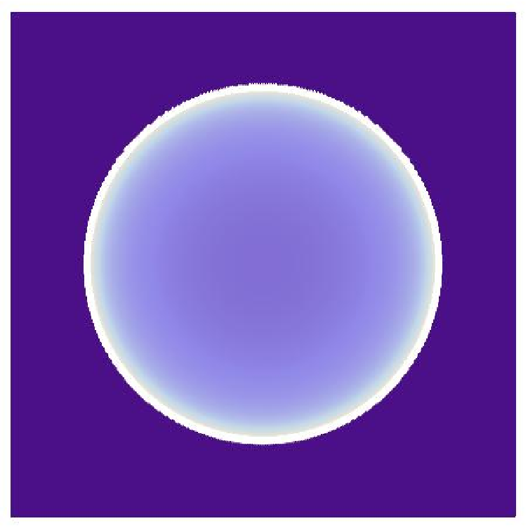
Figure 7. Density profile for the trivial initial data. The dark color corresponds to ρi,j,k=0\rho_{i,j,k}=0 and brighter color to larger ρi,j,k\rho_{i,j,k}. The scale of colors is arbitrary.

The standard explanation for the arctic circle in the uniform initial data case is that the dimer configurations that contribute to the partition function Ti,j,kT_{i,j,k} tend to be in a fundamental crystalline state in the vicinity of the corners of the square domain |i|+|j|≤|k||i|+|j|\leq|k|. There are four distinct such states, each corresponding to a (N,S,E,W) corner, characterized by an occupation number Di,j=1D_{i,j}=1 on each face (i,j)(i,j) (see Fig.5). Away from the corners, the dimer model has a non-trivial entropy, and the competition between order and disorder gives rise to a separating critical curve in the continuum thermodynamic limit when k→∞k\to\infty with ik=u\frac{i}{k}=u and jk=v\frac{j}{k}=v fixed, between a frozen phase (next to the corners) and a so-called temperate phase (in the center). Outside of the critical curve, the density decays exponentially as k→∞k\to\infty to 00, as each square tends to be occupied by a single dimer, while inside the curve it decreases as a power law ∝1k\propto\frac{1}{k}, whereas the coefficient tends to the non-zero function 2/(π​1−2​(u2+v2))2/(\pi\sqrt{1-2(u^{2}+v^{2})}), singular on the arctic curve. This function indicates a growing local disorder in the dimer configurations, maximum at the center of the Aztec domain. We have represented the values of the rescaled density function k​|ρi,j,k(0,0)|k|\rho_{i,j,k}^{(0,0)}| for fixed k=85k=85, −k≤i,j≤k-k\leq i,j\leq k and i+j+k=1i+j+k=1 mod 2.

3.4.2. 2×22\times 2 periodic case

To understand the emergence of a new (facet) central phase, let us first consider the simple case σ=0\sigma=0. We saw that in that case, the arctic curve degenerates to an inscribed square and the temperate region disappears. This is attained for instance by fixing b,c,d>0b,c,d>0 and letting a→0a\to 0 in the various density functions.

Refer to caption
Figure 8. The typical dominant dimer configurations for odd kk when a→0a\to 0: each aa-type face is occupied by two dimers, with two arbitrary choices of orientation on each aa-type face.

It is clear that if aa is very small, the Boltzmann weight of maximally occupied dimer configurations around the aa faces becomes the dominant contribution to the partition function (see Fig.8 for an illustration). We expect therefore a phase where the aa type faces are occupied by two dimers, with arbitrary (vertical or horizontal) orientation. This phase is globally crystalline, from the pinning of the dimers to the aa-type faces that form a square sublattice, but retains some non-trivial entropy, from the arbitrary orientation of the pair of dimers at each site, hence the name facet. Note that this also imposes another square sublattice of empty faces. The corresponding value of ⟨1−D⟩\langle 1-D\rangle for kk odd is −1-1 on the former sublattice, and 11 on the latter.

Refer to caption
Figure 9. The typical dominant dimer configurations for k=7k=7 when a→0a\to 0: each aa-type face in the inscribed square region is occupied by two dimers, with two arbitrary choices of orientation on each aa-type face (shaded).

More precisely, for σ=0\sigma=0 the solution of the system (3.4) and its companion for ϵ=η=1\epsilon=\eta=1 above lead to:

ρ(0,0)​(x,y,z)\displaystyle\rho^{(0,0)}(x,y,z) =\displaystyle= z(x​y−z2)​(x−y​z2)​(y−x​z2)​(1−x​y​z2)×\displaystyle\frac{z}{(xy-z^{2})(x-yz^{2})(y-xz^{2})(1-xyz^{2})}\times
{x2y2−xyz2−x3yz2−x2y2z2−xy3z2−x3y3z2−x2yz3−xy2z3−x3y2z3\displaystyle\left\{x^{2}y^{2}-xyz^{2}-x^{3}yz^{2}-x^{2}y^{2}z^{2}-xy^{3}z^{2}-x^{3}y^{3}z^{2}-x^{2}yz^{3}-xy^{2}z^{3}-x^{3}y^{2}z^{3}\right.
−x2y3z3+x2z4+x2y2z4+x2y4z4+x2yz5+xy2z5+x3y2z5+x2y3z5+x2y2z6}\displaystyle\left.-x^{2}y^{3}z^{3}+x^{2}z^{4}+x^{2}y^{2}z^{4}+x^{2}y^{4}z^{4}+x^{2}yz^{5}+xy^{2}z^{5}+x^{3}y^{2}z^{5}+x^{2}y^{3}z^{5}+x^{2}y^{2}z^{6}\right\}
+τ​z3​(x2−y2)​(1−x2​y2)(x​y−z2)​(x−y​z2)​(y−x​z2)​(1−x​y​z2)\displaystyle+\tau\frac{z^{3}(x^{2}-y^{2})(1-x^{2}y^{2})}{(xy-z^{2})(x-yz^{2})(y-xz^{2})(1-xyz^{2})}

and:

ρ(1,1)​(x,y,z)x​y\displaystyle\frac{\rho^{(1,1)}(x,y,z)}{xy} =\displaystyle= z(x​y−z2)​(x−y​z2)​(y−x​z2)​(1−x​y​z2)×\displaystyle\frac{z}{(xy-z^{2})(x-yz^{2})(y-xz^{2})(1-xyz^{2})}\times
{x2y2+x2yz+xy2z+x3y2z+x2y3z+y2z2+x2y2z2+x4y2z2−x2yz3\displaystyle\left\{x^{2}y^{2}+x^{2}yz+xy^{2}z+x^{3}y^{2}z+x^{2}y^{3}z+y^{2}z^{2}+x^{2}y^{2}z^{2}+x^{4}y^{2}z^{2}-x^{2}yz^{3}\right.
−xy2z3−x3y2z3−x2y3z3−xyz4−x3yz4−x2y2z4−xy3z4−x3y3z4+x2y2z6}\displaystyle\left.-xy^{2}z^{3}-x^{3}y^{2}z^{3}-x^{2}y^{3}z^{3}-xyz^{4}-x^{3}yz^{4}-x^{2}y^{2}z^{4}-xy^{3}z^{4}-x^{3}y^{3}z^{4}+x^{2}y^{2}z^{6}\right\}
−τ​z3​(x2−y2)​(1−x2​y2)(x​y−z2)​(x−y​z2)​(y−x​z2)​(1−x​y​z2)\displaystyle-\tau\frac{z^{3}(x^{2}-y^{2})(1-x^{2}y^{2})}{(xy-z^{2})(x-yz^{2})(y-xz^{2})(1-xyz^{2})}

with τ=c2c2+d2\tau=\frac{c^{2}}{c^{2}+d^{2}}. As explained above, the final generating function for ⟨1−Di,j⟩0,0,2​k−1\langle 1-D_{i,j}\rangle_{0,0,2k-1} for i+ji+j even is obtained by extracting the even powers of x,yx,y from ρ(0,0)\rho^{(0,0)} and the odd powers of x,yx,y from ρ(1,1)/(x​y)\rho^{(1,1)}/(xy), namely by forming:

U⁡(x,y,z)\displaystyle U(x,y,z) =\displaystyle= 14​(A⁡(x,y,z)+A⁡(−x,y,z)+A⁡(x,−y,z)+A⁡(−x,−y,z))\displaystyle\frac{1}{4}(A(x,y,z)+A(-x,y,z)+A(x,-y,z)+A(-x,-y,z))
+14​(B⁡(x,y,z)−B⁡(−x,y,z)−B⁡(x,−y,z)+B⁡(−x,−y,z))\displaystyle+\frac{1}{4}(B(x,y,z)-B(-x,y,z)-B(x,-y,z)+B(-x,-y,z))

where A=ρ(0,0)A=\rho^{(0,0)}, and B=ρ(1,1)/(x​y)B=\rho^{(1,1)}/(xy) above. Similarly, the generating function for ⟨1−Di,j⟩1,1,2​k\langle 1-D_{i,j}\rangle_{1,1,2k} for i+ji+j even is obtained by extracting the odd powers of x,yx,y from ρ(0,0)\rho^{(0,0)} and the even powers of x,yx,y from ρ(1,1)/(x​y)\rho^{(1,1)}/(xy), namely by forming:

V⁡(x,y,z)\displaystyle V(x,y,z) =\displaystyle= 14​(A⁡(x,y,z)−A⁡(−x,y,z)−A⁡(x,−y,z)+A⁡(−x,−y,z))\displaystyle\frac{1}{4}(A(x,y,z)-A(-x,y,z)-A(x,-y,z)+A(-x,-y,z))
+14​(B⁡(x,y,z)+B⁡(−x,y,z)+B⁡(x,−y,z)+B⁡(−x,−y,z))\displaystyle+\frac{1}{4}(B(x,y,z)+B(-x,y,z)+B(x,-y,z)+B(-x,-y,z))

Let us denote by fk​(x,y)f_{k}(x,y) the coefficient of zkz^{k} in the series expansion of f⁡(x,y,z)f(x,y,z), and by [n]x=xn−x−nx−x−1[n]_{x}=\frac{x^{n}-x^{-n}}{x-x^{-1}} and similarly for yy. Noting the generating functions

∑n≥0[n]x​[n]y​zn\displaystyle\sum_{n\geq 0}[n]_{x}[n]_{y}z^{n} =\displaystyle= x2​y2​z​(1−z2)(x​y−z2)​(x−y​z2)​(y−x​z2)​(1−x​y​z2)\displaystyle\frac{x^{2}y^{2}z(1-z^{2})}{(xy-z^{2})(x-yz^{2})(y-xz^{2})(1-xyz^{2})}
∑n≥1[n+1]x​[n−1]y​zn\displaystyle\sum_{n\geq 1}[n+1]_{x}[n-1]_{y}z^{n} =\displaystyle= y​z2​(y+x2​y+x4​y−x​z−x3​z−x​y2​z−x3​y2​z+x2​y​z2)(x​y−z2)​(x−y​z2)​(y−x​z2)​(1−x​y​z2)\displaystyle\frac{yz^{2}(y+x^{2}y+x^{4}y-xz-x^{3}z-xy^{2}z-x^{3}y^{2}z+x^{2}yz^{2})}{(xy-z^{2})(x-yz^{2})(y-xz^{2})(1-xyz^{2})}

and expressing U⁡(x,y,z)U(x,y,z) and V⁡(x,y,z)V(x,y,z) in terms of these, we finally get:

U4​k−1​(x,y)\displaystyle U_{4k-1}(x,y) =\displaystyle= [2​k]x​[2​k]y−[2​k−1]x​[2​k−1]y\displaystyle[2k]_{x}[2k]_{y}-[2k-1]_{x}[2k-1]_{y}
U4​k−3​(x,y)\displaystyle U_{4k-3}(x,y) =\displaystyle= τ⁡([2​k−2]x​[2​k]y−[2​k−3]x​[2​k−1]y)\displaystyle\tau([2k-2]_{x}[2k]_{y}-[2k-3]_{x}[2k-1]_{y})
+(1−τ)​([2​k]x​[2​k−2]y−[2​k−1]x​[2​k−3]y)\displaystyle\qquad+(1-\tau)([2k]_{x}[2k-2]_{y}-[2k-1]_{x}[2k-3]_{y})
V4​k−1​(x,y)\displaystyle V_{4k-1}(x,y) =\displaystyle= τ⁡([2​k−1]x​[2​k+1]y−[2​k−2]x​[2​k]y)\displaystyle\tau([2k-1]_{x}[2k+1]_{y}-[2k-2]_{x}[2k]_{y})
+(1−τ)​([2​k+1]x​[2​k−1]y−[2​k]x​[2​k−2]y)\displaystyle\qquad+(1-\tau)([2k+1]_{x}[2k-1]_{y}-[2k]_{x}[2k-2]_{y})
V4​k−3​(x,y)\displaystyle V_{4k-3}(x,y) =\displaystyle= [2​k−1]x​[2​k−1]y−[2​k−2]x​[2​k−2]y\displaystyle[2k-1]_{x}[2k-1]_{y}-[2k-2]_{x}[2k-2]_{y}

Recall that the UU’s correspond to the averages in the dimer model on Aztec graphs with a central face of aa type, while the VV’s correspond to the averages in the dimer model on Aztec graphs with a central face of bb type. The case U4​k−1,V4​k−3U_{4k-1},V_{4k-3} display an alternance of ±1\pm 1 on (even, even)/(odd,odd) faces. This is in agreement with the typical dominant configuration represented in Fig.9, corresponding to U7​(x,y)U_{7}(x,y): the facet occupies exactly the inscribed square |i|,|j|≤3|i|,|j|\leq 3, while outside this domain each face is occupied by a single dimer, i.e. we have four corners frozen in their respective fundamental states with zero entropy. The cases U4​k−3,V4​k−1U_{4k-3},V_{4k-1} also have a central facet square region with the same alternance of ±1\pm 1, but have a thin boundary region around the square where the averages explicitly depend on τ\tau.

We conclude that asymptotically the density is identically zero outside of the inscribed square |u|,|v|≤12|u|,|v|\leq\frac{1}{2}, while inside it takes finite nonzero values that alternate on two square sublattices. The arctic curve is nothing but the exact phase separation, here reduced to the inscribed square |u|=12,|v|≤12|u|=\frac{1}{2},|v|\leq\frac{1}{2} and |v|=12,|u|≤12|v|=\frac{1}{2},|u|\leq\frac{1}{2}.

Refer to caption = α 1 = α 0.98 = α 0.5 = α 0.01

Figure 10. Density profiles for ρi,j,k\rho_{i,j,k} for the periodic initial data corresponding to different values of α\alpha. We fixed b=c=d=1b=c=d=1 and vary aa accordingly to get the α\alpha shown in the profiles (see (3.5))

More generally, when 1>σ,τ>01>\sigma,\tau>0, we still expect frozen corner phases and a central facet phase induced by the pinning on one sublattice of configurations of pairs of parallel dimers, corresponding to the smallest weights among a,ba,b and c,dc,d. The plot of the arctic curve (3.8) shows that a disordered phase separates the facet from the frozen corners. In both the frozen corners and the facet, the convergence of ρi,j,k\rho_{i,j,k} for i/k=u,j/k=vi/k=u,j/k=v fixed is exponential in kk. As explained above, the behavior of ρ(0,0)\rho^{(0,0)} in the disordered phase is connected to the singularity x=y=z=1x=y=z=1 of both numerator (3.7) and denominator (3.6). We find that the leading orders in the tt expansion for x→1−t​x,y→1−t​y,z→1−t​zx\to 1-tx,y\to 1-ty,z\to 1-tz are respectively Q(0,0)∼tQ^{(0,0)}\sim t if σ≠12\sigma\neq\frac{1}{2}, and Q(0,0)∼t2Q^{(0,0)}\sim t^{2} otherwise, while D∼t4D\sim t^{4} in all cases. We deduce that if σ=12\sigma=\frac{1}{2} then ρi,j,k\rho_{i,j,k} for i/k=u,j/k=vi/k=u,j/k=v fixed tends to 00 algebraically, as k−1k^{-1}, and diverges at the boundary of the temperate zone (both along the facet border and the frozen corners border). However if σ≠12\sigma\neq\frac{1}{2}, we find that ρi,j,k\rho_{i,j,k} tends to a scaling function without any global rescaling. We display in Fig.10 a picture of the values of |ρi,j,k(0,0)||\rho_{i,j,k}^{(0,0)}| for size k=85k=85, −k≤i,j≤k-k\leq i,j\leq k and both ii and jj even.

4. Toroidal initial data II: the mm-toroidal case

In this section, we introduce the TT-system with initial data wrapped on a torus involving 4​m4m arbitrary initial values. This particular choice is exactly solvable, and leads to the exact derivation of higher degree arctic curves.

4.1. Exact solution of the TT-system with mm-toroidal initial data

Definition 4.1.

Let us consider the following condition on the initial data {ti,j}i,j∈ℤ\{t_{i,j}\}_{i,j\in{\mathbb{Z}}} of the TT-system (2.1):

(4.1) ti+m,j−m=ti,jandti+2,j+2=ti,j(i,j∈ℤ)t_{i+m,j-m}=t_{i,j}\qquad{\rm and}\qquad t_{i+2,j+2}=t_{i,j}\qquad(i,j\in{\mathbb{Z}})

Initial data with this property will be called mm-toroidal boundary conditions. The corresponding torus of the ℤ2{\mathbb{Z}}^{2} plane is generated by the two vectors e→1=(m,−m,0)\vec{e}_{1}=(m,-m,0) and e→2=(2,2,0)\vec{e}_{2}=(2,2,0).

It is easy to show that any solution of the TT-system with mm-toroidal boundary conditions satisfies the same toroidal conditions, namely that: Ti+m,j−m,k=Ti,j,kT_{i+m,j-m,k}=T_{i,j,k} and Ti+2,j+2,k=Ti,j,kT_{i+2,j+2,k}=T_{i,j,k} for all i,j∈ℤi,j\in{\mathbb{Z}} and k∈ℤ+k\in{\mathbb{Z}}_{+}, and i+j+k=1i+j+k=1 mod 2.

Quite remarkably, there is an explicit expression for the solution of the TT-system for mm-toroidal boundary conditions.

Refer to caption
Figure 11. The initial data of the mm-toroidal TT-system in the (i,j)(i,j) plane. The empty circles correspond to k=0k=0 and the filled circles to k=1k=1. We have shaded a fundamental domain for the corresponding torus.

Let us first denote respectively by ai,bi,ci,dia_{i},b_{i},c_{i},d_{i} the initial data corresponding to a fundamental domain in the planes k=0k=0 and k=1k=1, namely (see Fig.11 for an illustration):

ai\displaystyle a_{i} =\displaystyle= Ti+1,−i,0=ti+1,−ibi=Ti+2,−i+1,0=ti+2,−i+1\displaystyle T_{i+1,-i,0}=t_{i+1,-i}\qquad b_{i}=T_{i+2,-i+1,0}=t_{i+2,-i+1}
(4.2) ci\displaystyle c_{i} =\displaystyle= Ti,−i,1=ti,−idi=Ti+1,−i+1,1=ti+1,−i+1\displaystyle T_{i,-i,1}=t_{i,-i}\qquad\quad d_{i}=T_{i+1,-i+1,1}=t_{i+1,-i+1}

for i∈ℤi\in{\mathbb{Z}}. The sequences ai,bi,ci,dia_{i},b_{i},c_{i},d_{i} i∈ℤi\in{\mathbb{Z}} are clearly periodic with period mm, as a direct consequence of the conditions (4.1). Let us further introduce two mm-periodic sequences xi,yix_{i},y_{i} defined as:

(4.3) xi=ci​di+1+ci+1​diai​biandyi=ai−1​bi+ai​bi−1ci​di(i∈ℤ)x_{i}=\frac{c_{i}d_{i+1}+c_{i+1}d_{i}}{a_{i}b_{i}}\qquad{\rm and}\qquad y_{i}=\frac{a_{i-1}b_{i}+a_{i}b_{i-1}}{c_{i}d_{i}}\quad(i\in{\mathbb{Z}})

Note that we have:

Ti+1,−i,2=xi​biTi+2,−i+1,2=xi​aiT_{i+1,-i,2}=x_{i}b_{i}\qquad T_{i+2,-i+1,2}=x_{i}a_{i}

We also define for n≥1n\geq 1 and i∈ℤi\in{\mathbb{Z}} the quantities:

(4.4) un,i=∏ℓ=0n−1(xi−ℓ−1)n+12−|n−12−ℓ|vn,i=∏ℓ=0n−1(yi−ℓ−1)n+12−|n−12−ℓ|u_{n,i}=\prod_{\ell=0}^{n-1}\left(x_{i-\ell-1}\right)^{\frac{n+1}{2}-\big|\frac{n-1}{2}-\ell\big|}\qquad v_{n,i}=\prod_{\ell=0}^{n-1}\left(y_{i-\ell-1}\right)^{\frac{n+1}{2}-\big|\frac{n-1}{2}-\ell\big|}

with the convention that u0,i=u−1,i=u−2,i=1u_{0,i}=u_{-1,i}=u_{-2,i}=1 and similarly for vv. Finally, let θi,j,k\theta_{i,j,k} be defined for i,j∈ℤi,j\in{\mathbb{Z}} and k∈ℤ+k\in{\mathbb{Z}}_{+} as:

(4.5) θi,j,k=Ti+⌊k2⌋,j+⌊k2⌋,k​mod​ 2\theta_{i,j,k}=T_{i+\lfloor\frac{k}{2}\rfloor,j+\lfloor\frac{k}{2}\rfloor,k\,{\rm mod}\,2}

In particular, for k=0,1k=0,1 we have from the initial data (2.2):

(4.6) θi,j,i+j+1​mod​ 2=ti,j.\theta_{i,j,i+j+1\,{\rm mod}\,2}=t_{i,j}.

With the above definitions, the following theorem gives the exact value of the solution Ti,j,kT_{i,j,k} of the TT-system with mm-toroidal boundary conditions.

Theorem 4.2.

With the above definitions for un,i,vn,i,θi,j,ku_{n,i},v_{n,i},\theta_{i,j,k}, the solution Ti,j,kT_{i,j,k} to the TT-system with mm-toroidal boundary conditions (4.1) given by (4.2) reads explicitly:

(4.7) Ti,j,k=uk−1,i−j+k−12​vk−2,i−j+k−12​θi,j,kT_{i,j,k}=u_{k-1,\frac{i-j+k-1}{2}}\,v_{k-2,\frac{i-j+k-1}{2}}\,\theta_{i,j,k}

Moreover, we have the following explicit values for the cross-ratios Li,j,kL_{i,j,k} and Ri,j,kR_{i,j,k}, with the notations α=i−j2{\alpha}=\frac{i-j}{2}, β=i−j−12\beta=\frac{i-j-1}{2}, and δi,j[p]=δi−j,0​mod​p\delta^{[p]}_{i,j}=\delta_{i-j,0\,{\rm mod}\,p}:

Li,j,k\displaystyle L_{i,j,k} =\displaystyle= Ti+1,j,k​Ti−1,j,kTi,j,k+1​Ti,j,k−1=δi+j+k,0[4]​(δk,0[2]​aα​bα−1aα​bα−1+aα−1​bα+δk,1[2]​cβ+1​dβcβ​dβ+1+cβ+1​dβ)\displaystyle\frac{T_{i+1,j,k}T_{i-1,j,k}}{T_{i,j,k+1}T_{i,j,k-1}}=\delta^{[4]}_{i+j+k,0}\left(\delta^{[2]}_{k,0}\,\frac{a_{\alpha}b_{{\alpha}-1}}{a_{\alpha}b_{{\alpha}-1}+a_{{\alpha}-1}b_{{\alpha}}}+\delta^{[2]}_{k,1}\,\frac{c_{\beta+1}d_{\beta}}{c_{\beta}d_{\beta+1}+c_{\beta+1}d_{\beta}}\right)
+δi+j+k,2[4]​(δk,0[2]​aα−1​bαaα​bα−1+aα−1​bα+δk,1[2]​cβ​dβ+1cβ​dβ+1+cβ+1​dβ)\displaystyle\qquad\qquad\qquad\quad+\delta^{[4]}_{i+j+k,2}\left(\delta^{[2]}_{k,0}\,\frac{a_{{\alpha}-1}b_{{\alpha}}}{a_{\alpha}b_{{\alpha}-1}+a_{{\alpha}-1}b_{{\alpha}}}+\delta^{[2]}_{k,1}\,\frac{c_{\beta}d_{\beta+1}}{c_{\beta}d_{\beta+1}+c_{\beta+1}d_{\beta}}\right)
Ri,j,k\displaystyle R_{i,j,k} =\displaystyle= Ti,j+1,k​Ti,j−1,kTi,j,k+1​Ti,j,k−1=1−Li,j,k\displaystyle\frac{T_{i,j+1,k}T_{i,j-1,k}}{T_{i,j,k+1}T_{i,j,k-1}}=1-L_{i,j,k}
Proof.

For Ti,j,kT_{i,j,k} as in the statement of the theorem, let us compute the ratios Li,j,kL_{i,j,k} and Ri,j,kR_{i,j,k}. To this end, we note that by definition:

(4.8) uk,αuk−1,α=∏ℓ=0⌊k−12⌋xα−k+ℓanduk−1,α−1​uk−1,αuk−2,α−1​uk,α={1if​k​even1/xα−k+12otherwise\frac{u_{k,{\alpha}}}{u_{k-1,{\alpha}}}=\prod_{\ell=0}^{\lfloor\frac{k-1}{2}\rfloor}x_{{\alpha}-k+\ell}\quad{\rm and}\quad\frac{u_{k-1,{\alpha}-1}\,u_{k-1,{\alpha}}}{u_{k-2,{\alpha}-1}\,u_{k,{\alpha}}}=\left\{\begin{matrix}1&{\rm if}\,k\,{\rm even}\\ 1/x_{{\alpha}-\frac{k+1}{2}}&{\rm otherwise}\end{matrix}\right.

and similarly for vv:

(4.9) vk−2,α−1​vk−2,αvk−3,α−1​vk−1,α={1/yα−k2if​k​even1otherwise\frac{v_{k-2,{\alpha}-1}\,v_{k-2,{\alpha}}}{v_{k-3,{\alpha}-1}\,v_{k-1,{\alpha}}}=\left\{\begin{matrix}1/y_{{\alpha}-\frac{k}{2}}&{\rm if}\,k\,{\rm even}\\ 1&{\rm otherwise}\end{matrix}\right.

Let us pick i,j,ki,j,k such that i+j+k=0i+j+k=0 mod 2, and use the result for the cross-ratios of (4.8-4.9) for α=i−j+k2{\alpha}=\frac{i-j+k}{2}. Noting finally that

θi+1,j,2​k​θi−1,j,2​kθi,j,2​k+1​θi,j,2​k−1\displaystyle\frac{\theta_{i+1,j,2k}\theta_{i-1,j,2k}}{\theta_{i,j,2k+1}\theta_{i,j,2k-1}} =\displaystyle= {aα​bα−1cα​dαif​i+j+2​k2​evenaα−1​bαcα​dαotherwise(α=i−j2)\displaystyle\left\{\begin{matrix}\frac{a_{{\alpha}}b_{{\alpha}-1}}{c_{\alpha}d_{\alpha}}&{\rm if}\,\frac{i+j+2k}{2}\,{\rm even}\\ \frac{a_{{\alpha}-1}b_{{\alpha}}}{c_{\alpha}d_{\alpha}}&{\rm otherwise}\end{matrix}\right.\ \left({\alpha}=\frac{i-j}{2}\right)
θi+1,j,2​k−1​θi−1,j,2​k−1θi,j,2​k​θi,j,2​k−2\displaystyle\frac{\theta_{i+1,j,2k-1}\theta_{i-1,j,2k-1}}{\theta_{i,j,2k}\theta_{i,j,2k-2}} =\displaystyle= {cβ​dβ+1aβ​bβif​i+j+2​k−12​evencβ+1​dβaβ​bβotherwise(β=i−j−12)\displaystyle\left\{\begin{matrix}\frac{c_{\beta}d_{\beta+1}}{a_{\beta}b_{\beta}}&{\rm if}\,\frac{i+j+2k-1}{2}\,{\rm even}\\ \frac{c_{\beta+1}d_{\beta}}{a_{\beta}b_{\beta}}&{\rm otherwise}\end{matrix}\right.\left(\beta=\frac{i-j-1}{2}\right)

we conclude that

Li,j,2​k\displaystyle L_{i,j,2k} =\displaystyle= {aα​bα−1aα​bα−1+aα−1​bαif​i+j+2​k=0​mod​ 4aα−1​bαaα​bα−1+aα−1​bαif​i+j+2​k=2​mod​ 4(α=i−j2)\displaystyle\left\{\begin{matrix}\frac{a_{\alpha}b_{{\alpha}-1}}{a_{\alpha}b_{{\alpha}-1}+a_{{\alpha}-1}b_{{\alpha}}}&\ {\rm if}\ i+j+2k=0\,{\rm mod}\,4\\ \frac{a_{{\alpha}-1}b_{{\alpha}}}{a_{\alpha}b_{{\alpha}-1}+a_{{\alpha}-1}b_{{\alpha}}}&\ {\rm if}\ i+j+2k=2\,{\rm mod}\,4\\ \end{matrix}\right.\qquad\left(\alpha=\frac{i-j}{2}\right)
Li,j,2​k−1\displaystyle L_{i,j,2k-1} =\displaystyle= {cβ+1​dβcβ​dβ+1+cβ+1​dβif​i+j+2​k−1=0​mod​ 4cβ​dβ+1cβ​dβ+1+cβ+1​dβif​i+j+2​k−1=2​mod​ 4(β=i−j−12)\displaystyle\left\{\begin{matrix}\frac{c_{\beta+1}d_{\beta}}{c_{\beta}d_{\beta+1}+c_{\beta+1}d_{\beta}}&\ {\rm if}\ i+j+2k-1=0\,{\rm mod}\,4\\ \frac{c_{\beta}d_{\beta+1}}{c_{\beta}d_{\beta+1}+c_{\beta+1}d_{\beta}}&\ {\rm if}\ i+j+2k-1=2\,{\rm mod}\,4\\ \end{matrix}\right.\left(\beta=\frac{i-j-1}{2}\right)

Similarly we compute the quantities:

Ri,j,2​k\displaystyle R_{i,j,2k} =\displaystyle= {aα−1​bαaα​bα−1+aα−1​bαif​i+j+2​k=0​mod​ 4aα​bα−1aα​bα−1+aα−1​bαif​i+j+2​k=2​mod​ 4(α=i−j2)\displaystyle\left\{\begin{matrix}\frac{a_{{\alpha}-1}b_{{\alpha}}}{a_{\alpha}b_{{\alpha}-1}+a_{{\alpha}-1}b_{{\alpha}}}&\ {\rm if}\ i+j+2k=0\,{\rm mod}\,4\\ \frac{a_{\alpha}b_{{\alpha}-1}}{a_{\alpha}b_{{\alpha}-1}+a_{{\alpha}-1}b_{{\alpha}}}&\ {\rm if}\ i+j+2k=2\,{\rm mod}\,4\\ \end{matrix}\right.\qquad\left(\alpha=\frac{i-j}{2}\right)
Ri,j,2​k−1\displaystyle R_{i,j,2k-1} =\displaystyle= {cβ​dβ+1cβ​dβ+1+cβ+1​dβif​i+j+2​k−1=0​mod​ 4cβ+1​dβcβ​dβ+1+cβ+1​dβif​i+j+2​k−1=2​mod​ 4(β=i−j−12)\displaystyle\left\{\begin{matrix}\frac{c_{\beta}d_{\beta+1}}{c_{\beta}d_{\beta+1}+c_{\beta+1}d_{\beta}}&\ {\rm if}\ i+j+2k-1=0\,{\rm mod}\,4\\ \frac{c_{\beta+1}d_{\beta}}{c_{\beta}d_{\beta+1}+c_{\beta+1}d_{\beta}}&\ {\rm if}\ i+j+2k-1=2\,{\rm mod}\,4\\ \end{matrix}\right.\left(\beta=\frac{i-j-1}{2}\right)

We conclude that Ri,j,k+Li,j,k=1R_{i,j,k}+L_{i,j,k}=1 for all k≥0k\geq 0 and i,j∈ℤi,j\in{\mathbb{Z}}, and therefore Ti,j,kT_{i,j,k} satisfies the TT-system (2.1). Moreover, the initial values of Ti,j,kT_{i,j,k} are Ti,j,i+j+1​mod​ 2=θi,j,i+j+1​mod​ 2=ti,jT_{i,j,i+j+1\,{\rm mod}\,2}=\theta_{i,j,i+j+1\,{\rm mod}\,2}=t_{i,j} by (4.6). The theorem follows. ∎

Example 4.3.

For m=1m=1, all sequences are constant, ai=aa_{i}=a, bi=bb_{i}=b, ci=cc_{i}=c, di=dd_{i}=d, and xi=2​a​bc​d=xx_{i}=\frac{2ab}{cd}=x, yi=2​c​da​b=yy_{i}=\frac{2cd}{ab}=y. Moreover, we have un,i=x⌊(n+1)24⌋u_{n,i}=x^{\lfloor\frac{(n+1)^{2}}{4}\rfloor}, vn,i=y⌊(n+1)24⌋v_{n,i}=y^{\lfloor\frac{(n+1)^{2}}{4}\rfloor}, hence:

Ti,j,k=2k⁡(k−1)2​(a​bc​d)⌊k2⌋​{δk,0[2]​(a​δi+j+k,1[4]+b​δi+j+k,3[4])+δk,1[2]​(c​δi+j+k,1[4]+d​δi+j+k,3[4])}T_{i,j,k}=2^{\frac{k(k-1)}{2}}\left(\frac{ab}{cd}\right)^{\lfloor\frac{k}{2}\rfloor}\left\{\delta^{[2]}_{k,0}\left(a\,\delta^{[4]}_{i+j+k,1}+b\,\delta^{[4]}_{i+j+k,3}\right)+\delta^{[2]}_{k,1}\left(c\,\delta^{[4]}_{i+j+k,1}+d\,\delta^{[4]}_{i+j+k,3}\right)\right\}

This solution is slightly more general that the uniform one (which would correspond to a=b=c=d=1a=b=c=d=1 and Ti,j,k=2k⁡(k−1)2T_{i,j,k}=2^{\frac{k(k-1)}{2}}), but we easily compute:

Ri,j,k=Li,j,k=12(i,j∈ℤ;k∈ℤ+;i+j+k=0mod 2),R_{i,j,k}=L_{i,j,k}=\frac{1}{2}\qquad(i,j\in{\mathbb{Z}};k\in{\mathbb{Z}}_{+};i+j+k=0\,{\rm mod}\,2)\,,

therefore the general equation (2.4) for the density reduces to that of the uniform case (2.8).

Example 4.4.

For m=2m=2, we find that

x0=c1​d0+c0​d1a0​b0,x1=c1​d0+c0​d1a1​b1,y0=a0​b1+a1​b0c0​d0,y1=a0​b1+a1​b0c1​d1.x_{0}=\frac{c_{1}d_{0}+c_{0}d_{1}}{a_{0}b_{0}},\quad x_{1}=\frac{c_{1}d_{0}+c_{0}d_{1}}{a_{1}b_{1}},\quad y_{0}=\frac{a_{0}b_{1}+a_{1}b_{0}}{c_{0}d_{0}},\quad y_{1}=\frac{a_{0}b_{1}+a_{1}b_{0}}{c_{1}d_{1}}.

and the solution reads:

Ti,j,k\displaystyle T_{i,j,k} =\displaystyle= δk,0[2]​(ai−j−12​δi+j+k,1[4]+bi−j−12​δi+j+k,3[4])​(x0​x1​y0​y1)k⁡(k−2)8​(xi−j−12)⌊k+24⌋​(xi−j+12)⌊k4⌋\displaystyle\delta_{k,0}^{[2]}\left(a_{\frac{i-j-1}{2}}\,\delta_{i+j+k,1}^{[4]}+b_{\frac{i-j-1}{2}}\,\delta_{i+j+k,3}^{[4]}\right)(x_{0}x_{1}y_{0}y_{1})^{\frac{k(k-2)}{8}}\left(x_{\frac{i-j-1}{2}}\right)^{\lfloor\frac{k+2}{4}\rfloor}\left(x_{\frac{i-j+1}{2}}\right)^{\lfloor\frac{k}{4}\rfloor}
+\displaystyle+ δk,1[2]​(ci−j2​δi+j+k,1[4]+di−j2​δi+j+k,3[4])​(x0​x1​y0​y1)k2−18​(yi−j2)−⌊k−14⌋​(yi−j2+1)−⌊k+14⌋\displaystyle\delta_{k,1}^{[2]}\left(c_{\frac{i-j}{2}}\,\delta_{i+j+k,1}^{[4]}+d_{\frac{i-j}{2}}\,\delta_{i+j+k,3}^{[4]}\right)(x_{0}x_{1}y_{0}y_{1})^{\frac{k^{2}-1}{8}}\left(y_{\frac{i-j}{2}}\right)^{-\lfloor\frac{k-1}{4}\rfloor}\left(y_{\frac{i-j}{2}+1}\right)^{-\lfloor\frac{k+1}{4}\rfloor}

Again, this solution is more general than that of the 2×22\times 2 case (3.2) (which would correspond to c0=d1=ac_{0}=d_{1}=a, c1=d0=bc_{1}=d_{0}=b, a1=b0=ca_{1}=b_{0}=c, and a0=b1=da_{0}=b_{1}=d), but as we shall see below (Example 4.8), it has the same values of Ri,j,kR_{i,j,k} and Li,j,kL_{i,j,k} and therefore the same equation for the density.

4.2. Density: exact derivation

In this section we consider the TT-system with mm-toroidal boundary conditions. We define the density ρ≡ρ(0,0)\rho\equiv\rho^{(0,0)} as before as the response of the system to an infinitesimal perturbation of the initial data at position (0,0)(0,0), with value T0,0,1=t0,0=c0T_{0,0,1}=t_{0,0}=c_{0}. More precisely, we write:

ρi,j,k=c0​∂Log​Ti,j,k∂t0,0|t0,0=c0\rho_{i,j,k}=c_{0}\frac{\partial{\rm Log}\,T_{i,j,k}}{\partial t_{0,0}}\Big|_{t_{0,0}=c_{0}}

Our aim in this section is to compute ρi,j,k\rho_{i,j,k} explicitly (As before, the singularity locus of the generating function for ρ\rho will determine the suitable arctic curve.). Note that we have the following initial conditions:

(4.10) ρi,j,0=0andρi,j,1=δi,0​δj,0(i,j∈ℤ)\rho_{i,j,0}=0\qquad{\rm and}\qquad\rho_{i,j,1}=\delta_{i,0}\delta_{j,0}\qquad(i,j\in{\mathbb{Z}})

Next, differentiating the TT-system relation w.r.t. to t0,0t_{0,0} provides us with the following system of linear recursion relations for ρi,j,k\rho_{i,j,k}:

(4.11) ρi,j,k+1+ρi,j,k−1=Li,j,k​(ρi+1,j,k+ρi−1,j,k)+Ri,j,k​(ρi,j+1,k+ρi,j−1,k)\rho_{i,j,k+1}+\rho_{i,j,k-1}=L_{i,j,k}(\rho_{i+1,j,k}+\rho_{i-1,j,k})+R_{i,j,k}(\rho_{i,j+1,k}+\rho_{i,j-1,k})

which, together with the initial conditions (4.10), determine ρi,j,k\rho_{i,j,k} entirely. The crucial remark here is that although this system is infinite, it has only finitely many distinct coefficients. Indeed, from Theorem 4.2, we deduce the following simple:

Corollary 4.5.

The quantities (Li,j,k,Ri,j,k)(L_{i,j,k},R_{i,j,k}) for the solutions of the TT-system with mm-toroidal boundary conditions have the following periodicities:

Li+2,j+2,k\displaystyle L_{i+2,j+2,k} =\displaystyle= Li,j,kLi+m,j−m,k=Li,j,kLi+1,j+1,k+2=Li,j,k\displaystyle L_{i,j,k}\qquad L_{i+m,j-m,k}=L_{i,j,k}\qquad L_{i+1,j+1,k+2}=L_{i,j,k}
Ri+2,j+2,k\displaystyle R_{i+2,j+2,k} =\displaystyle= Ri,j,kRi+m,j−m,k=Ri,j,kRi+1,j+1,k+2=Ri,j,k\displaystyle R_{i,j,k}\qquad R_{i+m,j-m,k}=R_{i,j,k}\qquad R_{i+1,j+1,k+2}=R_{i,j,k}
Proof.

The first two relations are clear, as this periodicity is inherited from that of the initial data (4.1). The last one is checked directly on the expressions for Li,j,k,Ri,j,kL_{i,j,k},R_{i,j,k} of Theorem 4.2: one simply notices that the translation (i,j,k)→(i+1,j+1,k+2)(i,j,k)\to(i+1,j+1,k+2) leaves α{\alpha} and β\beta invariant, and leaves also the quantity i+j+k→i+j+k+4i+j+k\to i+j+k+4 invariant modulo 44, and k→k+2k\to k+2 invariant modulo 2. ∎

In other words, coefficients of the system (4.11) are periodic in the ℤ3{\mathbb{Z}}^{3} lattice, with period vectors: e→1=(2,2,0)\vec{e}_{1}=(2,2,0), e→2=(m,−m,0)\vec{e}_{2}=(m,-m,0) and e→3=(1,1,2)\vec{e}_{3}=(1,1,2). This suggests to introduce the following generating functions, for i,j∈ℤi,j\in{\mathbb{Z}} and k∈ℤ+k\in{\mathbb{Z}}_{+}:

ρ(i,j,k)​(x,y,z)=∑a,b∈ℤ,c≥0ρi+2​a+m​b+c,j+2​a−m​b+c,k+2​c​xi+2​a+m​b+c​yj+2​a−m​b+c​zk+2​c\rho^{(i,j,k)}(x,y,z)=\sum_{a,b\in{\mathbb{Z}},c\geq 0}\rho_{i+2a+mb+c,j+2a-mb+c,k+2c}x^{i+2a+mb+c}y^{j+2a-mb+c}z^{k+2c}

while the total density generating function ρ⁡(x,y,z)=∑i,j∈ℤ,k∈ℤ+xi​yj​zk​ρi,j,k\rho(x,y,z)=\sum_{i,j\in{\mathbb{Z}},k\in{\mathbb{Z}}_{+}}x^{i}y^{j}z^{k}\rho_{i,j,k} is equal to the sum

ρ⁡(x,y,z)=∑(i,j,k)∈Πmρ(i,j,k)​(x,y,z)\rho(x,y,z)=\sum_{(i,j,k)\in\Pi_{m}}\rho^{(i,j,k)}(x,y,z)

where Πm\Pi_{m} is the set of integral points within the paralellepipedon based on e→i\vec{e}_{i}, i=1,2,3i=1,2,3, namely:

Πm={∑i=13tie→i, 0≤ti<1}∩{(i,j,k)∈ℤ3,i+j+k=1mod 2}\Pi_{m}=\{\sum_{i=1}^{3}t_{i}\vec{e}_{i},\ 0\leq t_{i}<1\}\cap\{(i,j,k)\in{\mathbb{Z}}^{3},\ i+j+k=1\,{\rm mod}\,2\}

Note that with the above definition, ρ(i,j,k)​(x,y,z)\rho^{(i,j,k)}(x,y,z) is periodic in i,j,ki,j,k, namely it satisfies:

ρ(i+2​a+m​b+c,j+2​a−m​b+c,k+2​c)​(x,y,z)=ρ(i,j,k)​(x,y,z)\rho^{(i+2a+mb+c,j+2a-mb+c,k+2c)}(x,y,z)=\rho^{(i,j,k)}(x,y,z)

for a,b∈ℤa,b\in{\mathbb{Z}} and c∈ℤ+c\in{\mathbb{Z}}_{+}, for all i,j∈ℤi,j\in{\mathbb{Z}} and k∈ℤ+k\in{\mathbb{Z}}_{+}. For later use, we also note that, extending the above definition to k=−1k=-1 leads to:

ρ(i,j,−1)​(x,y,z)\displaystyle\rho^{(i,j,-1)}(x,y,z) =\displaystyle= −z−1​δi,0​δj,0+∑a,b∈ℤ,c≥1ρi+2​a+m​b+c,j+2​a−m​b+c,k+2​c​xi+2​a+m​b+c​yj+2​a−m​b+c​zk+2​c\displaystyle-z^{-1}\delta_{i,0}\delta_{j,0}+\sum_{a,b\in{\mathbb{Z}},c\geq 1}\rho_{i+2a+mb+c,j+2a-mb+c,k+2c}x^{i+2a+mb+c}y^{j+2a-mb+c}z^{k+2c}
=\displaystyle= −z−1​δi,0​δj,0+ρ(i+1,j+1,1)​(x,y,z)\displaystyle-z^{-1}\delta_{i,0}\delta_{j,0}+\rho^{(i+1,j+1,1)}(x,y,z)

where we have used ρi,j,1+ρi,j,−1=0\rho_{i,j,1}+\rho_{i,j,-1}=0 and the initial condition. We finally obtain the following system for the generating functions ρ(i,j,k)​(x,y,z)\rho^{(i,j,k)}(x,y,z), k=0,1k=0,1 by use of the periodicities:

Fori+j=0​mod​ 2:\displaystyle{\rm For}\ \ i+j=0\,{\rm mod}\,2:
z−1​ρ(i,j,1)​(x,y,z)+z​ρ(i+1,j+1,1)​(x,y,z)=Li,j,0​(x−1​ρ(i+1,j,0)​(x,y,z)+x​ρ(i−1,j,0)​(x,y,z))\displaystyle\quad z^{-1}\rho^{(i,j,1)}(x,y,z)+z\rho^{(i+1,j+1,1)}(x,y,z)=L_{i,j,0}(x^{-1}\rho^{(i+1,j,0)}(x,y,z)+x\rho^{(i-1,j,0)}(x,y,z))
+Ri,j,0​(y−1​ρ(i,j+1,0)​(x,y,z)+y​ρ(i,j−1,0)​(x,y,z))+δi,0​δj,0\displaystyle\qquad\qquad\qquad\qquad\qquad\qquad\qquad+R_{i,j,0}(y^{-1}\rho^{(i,j+1,0)}(x,y,z)+y\rho^{(i,j-1,0)}(x,y,z))+\delta_{i,0}\delta_{j,0}
Fori+j=1​mod​ 2:\displaystyle{\rm For}\ \ i+j=1\,{\rm mod}\,2:
z−1​ρ(i−1,j−1,0)​(x,y,z)+z​ρ(i,j,0)​(x,y,z)=Li,j,1​(x−1​ρ(i+1,j,1)​(x,y,z)+x​ρ(i−1,j,1)​(x,y,z))\displaystyle\quad z^{-1}\rho^{(i-1,j-1,0)}(x,y,z)+z\rho^{(i,j,0)}(x,y,z)=L_{i,j,1}(x^{-1}\rho^{(i+1,j,1)}(x,y,z)+x\rho^{(i-1,j,1)}(x,y,z))
+Ri,j,1​(y−1​ρ(i,j+1,1)​(x,y,z)+y​ρ(i,j−1,1)​(x,y,z))\displaystyle\qquad\qquad\qquad\qquad\qquad\qquad\qquad\qquad\qquad+R_{i,j,1}(y^{-1}\rho^{(i,j+1,1)}(x,y,z)+y\rho^{(i,j-1,1)}(x,y,z))

We may actually further restrict this system to a fundamental domain PmP_{m} of the (i,j,k)(i,j,k), k=0,1k=0,1 planes modulo e→1\vec{e}_{1} and e→2\vec{e}_{2}, which we take to be:

Pm={(i+1,−i,0),(i+2,−i+1,0),(i,−i,1),(i+1,−i+1,1)}i∈{0,1,…,m−1}P_{m}=\Big\{(i+1,-i,0),(i+2,-i+1,0),(i,-i,1),(i+1,-i+1,1)\Big\}_{i\in\{0,1,...,m-1\}}

Let us define the four following mm-periodic functions for i∈ℤi\in{\mathbb{Z}}:

αi​(x,y,z)\displaystyle\alpha_{i}(x,y,z) =\displaystyle= ρ(i+1,−i,0)​(x,y,z),βi​(x,y,z)=ρ(i+2,−i+1,0)​(x,y,z)\displaystyle\rho^{(i+1,-i,0)}(x,y,z),\qquad\beta_{i}(x,y,z)=\rho^{(i+2,-i+1,0)}(x,y,z)
γi​(x,y,z)\displaystyle\gamma_{i}(x,y,z) =\displaystyle= ρ(i,−i,1)​(x,y,z),δi​(x,y,z)=ρ(i+1,−i+1,1)​(x,y,z)\displaystyle\rho^{(i,-i,1)}(x,y,z),\qquad\quad\delta_{i}(x,y,z)=\rho^{(i+1,-i+1,1)}(x,y,z)

and the coefficients

(4.12) λi=Li,−i,0=ai​bi−1ai−1​bi+ai​bi−1μi=Li+2,−i+1,1=ci+1​dici​di+1+ci+1​di\lambda_{i}=L_{i,-i,0}=\frac{a_{i}b_{i-1}}{a_{i-1}b_{i}+a_{i}b_{i-1}}\qquad\mu_{i}=L_{i+2,-i+1,1}=\frac{c_{i+1}d_{i}}{c_{i}d_{i+1}+c_{i+1}d_{i}}

so that Li+1,−i+1,0=1−λiL_{i+1,-i+1,0}=1-\lambda_{i} and Li+3,−i+2,1=1−μiL_{i+3,-i+2,1}=1-\mu_{i}. Note also that, as is readily seen from their definition, these coefficients are not independent, as they must satisfy the relations:

(4.13) ∏i=0m−1(1λi−1)=∏i=0m−1(1μi−1)=1\prod_{i=0}^{m-1}\left(\frac{1}{\lambda_{i}}-1\right)=\prod_{i=0}^{m-1}\left(\frac{1}{\mu_{i}}-1\right)=1

We may summarize the above results into:

Theorem 4.6.

The density generating functions αi,βi,γi,δi{\alpha}_{i},\beta_{i},\gamma_{i},\delta_{i}, for i∈{0,1,…,m−1}i\in\{0,1,...,m-1\}, are uniquely determined as the solutions of the following 4​m×4​m4m\times 4m linear system:

z−1​αi+z​βi−λi​(x−1​γi+1+x​δi)−(1−λi)​(y−1​γi+y​δi+1)\displaystyle z^{-1}\,{\alpha}_{i}+z\,\beta_{i}-\lambda_{i}\,(x^{-1}\,\gamma_{i+1}+x\,\delta_{i})-(1-\lambda_{i})(y^{-1}\,\gamma_{i}+y\,\delta_{i+1}) =\displaystyle= 0\displaystyle 0
z−1​βi+z​αi−(1−λi)​(x−1​δi+1+x​γi)−λi​(y−1​δi+y​γi+1)\displaystyle z^{-1}\,\beta_{i}+z\,{\alpha}_{i}-(1-\lambda_{i})(x^{-1}\,\delta_{i+1}+x\,\gamma_{i})-\lambda_{i}\,(y^{-1}\,\delta_{i}+y\,\gamma_{i+1}) =\displaystyle= 0\displaystyle 0
z−1​γi+z​δi−μi​(x−1​αi+x​βi−1)−(1−μi)​(y−1​αi−1+y​βi)\displaystyle z^{-1}\,\gamma_{i}+z\,\delta_{i}-\mu_{i}\,(x^{-1}\,{\alpha}_{i}+x\,\beta_{i-1})-(1-\mu_{i})(y^{-1}\,{\alpha}_{i-1}+y\,\beta_{i}) =\displaystyle= δi,0\displaystyle\delta_{i,0}
(4.14) z−1​δi+z​γi−(1−μi)​(x−1​βi+x​αi−1)−μi​(y−1​βi−1+y​αi)\displaystyle z^{-1}\,\delta_{i}+z\,\gamma_{i}-(1-\mu_{i})(x^{-1}\,\beta_{i}+x\,{\alpha}_{i-1})-\mu_{i}\,(y^{-1}\,\beta_{i-1}+y\,{\alpha}_{i}) =\displaystyle= 0\displaystyle 0

for i,j∈{0,1,…,m−1}i,j\in\{0,1,...,m-1\}, subject to the periodicity conditions αm=α0{\alpha}_{m}={\alpha}_{0}, α−1=αm−1{\alpha}_{-1}={\alpha}_{m-1}, and similarly for the β\beta, γ\gamma, δ\delta’s.

The solution of the general system for the mm-periodic densities of Theorem 4.6 is always a rational fraction of x,y,zx,y,z, with denominator given by the determinant of the system (4.14). The matrix of coefficients may be rewritten in block form as:

M=(z−1​Iz​I−M⁡(x,y)−M¯​(y−1,x−1)z​Iz−1​I−M⁡(y−1,x−1)−M¯​(x,y)−P⁡(x,y)−P¯​(y−1,x−1)z−1​Iz​I−P¯​(x,y)−P⁡(y−1,x−1)z​Iz−1​I)M=\begin{pmatrix}z^{-1}\,I&zI&-M(x,y)&-{\bar{M}}(y^{-1},x^{-1})\\ z\,I&z^{-1}I&-M(y^{-1},x^{-1})&-{\bar{M}}(x,y)\\ -P(x,y)&-{\bar{P}}(y^{-1},x^{-1})&z^{-1}I&z\,I\\ -{\bar{P}}(x,y)&-P(y^{-1},x^{-1})&z\,I&z^{-1}I\end{pmatrix}

where all the entries are m×mm\times m matrices, with:

P⁡(x,y)=(μ0x00⋯01−μ0y1−μ1yμ1x0001−μ2yμ2x⋱0⋱⋱⋱⋱⋱⋱⋱00⋯⋯01−μm−1yμm−1x)P(x,y)=\begin{pmatrix}\frac{\mu_{0}}{x}&0&0&\cdots&0&\frac{1-\mu_{0}}{y}\\ \frac{1-\mu_{1}}{y}&\frac{\mu_{1}}{x}&0&&&0\\ 0&\frac{1-\mu_{2}}{y}&\frac{\mu_{2}}{x}&\ddots&&0\\ \vdots&\ddots&\ddots&\ddots&\ddots&\vdots\\ \vdots&&\ddots&\ddots&\ddots&0\\ 0&\cdots&\cdots&0&\frac{1-\mu_{m-1}}{y}&\frac{\mu_{m-1}}{x}\end{pmatrix}
M⁡(x,y)=(1−λ0yλ0x0⋯0001−λ1yλ1x⋱0001−λ2yλ2x⋱⋱⋱⋱⋱00⋱⋱⋱λm−2xλm−1x⋯⋯001−λm−1x)M(x,y)=\begin{pmatrix}\frac{1-\lambda_{0}}{y}&\frac{\lambda_{0}}{x}&0&\cdots&0&0\\ 0&\frac{1-\lambda_{1}}{y}&\frac{\lambda_{1}}{x}&\ddots&&0\\ 0&0&\frac{1-\lambda_{2}}{y}&\frac{\lambda_{2}}{x}&\ddots&\vdots\\ \vdots&\ddots&\ddots&\ddots&\ddots&0\\ 0&&\ddots&\ddots&\ddots&\frac{\lambda_{m-2}}{x}\\ \frac{\lambda_{m-1}}{x}&\cdots&\cdots&0&0&\frac{1-\lambda_{m-1}}{x}\end{pmatrix}

and P¯​(x,y){\bar{P}}(x,y) is P⁡(x,y)P(x,y) with μi\mu_{i} and 1−μi1-\mu_{i} interchanged, while M¯​(x,y){\bar{M}}(x,y) is M⁡(x,y)M(x,y) with λi\lambda_{i} and 1−λi1-\lambda_{i} interchanged.

Example 4.7.

For m=1m=1, the relation (4.13) gives λ0=μ0=12\lambda_{0}=\mu_{0}=\frac{1}{2} as expected. Moreover, denoting by α≡α0\alpha\equiv{\alpha}_{0}, etc., the linear system of Theorem 4.6 reduces to:

z−1​α+z​β−12​(x−1​γ+x​δ)−12​(y−1​γ+y​δ)\displaystyle z^{-1}\,{\alpha}+z\,\beta-\frac{1}{2}(x^{-1}\,\gamma+x\,\delta)-\frac{1}{2}(y^{-1}\,\gamma+y\,\delta) =\displaystyle= 0\displaystyle 0
z−1​β+z​α−12​(x−1​δ+x​γ)−12​(y−1​δ+y​γ)\displaystyle z^{-1}\,\beta+z\,{\alpha}-\frac{1}{2}(x^{-1}\,\delta+x\,\gamma)-\frac{1}{2}(y^{-1}\,\delta+y\,\gamma) =\displaystyle= 0\displaystyle 0
z−1​γ+z​δ−12​(x−1​α+x​β)−12​(y−1​α+y​β)\displaystyle z^{-1}\,\gamma+z\,\delta-\frac{1}{2}(x^{-1}\,{\alpha}+x\,\beta)-\frac{1}{2}(y^{-1}\,{\alpha}+y\,\beta) =\displaystyle= 1\displaystyle 1
z−1​δ+z​γ−12​(x−1​β+x​α)−12​(y−1​β+y​α)\displaystyle z^{-1}\,\delta+z\,\gamma-\frac{1}{2}(x^{-1}\,\beta+x\,{\alpha})-\frac{1}{2}(y^{-1}\,\beta+y\,{\alpha}) =\displaystyle= 0\displaystyle 0

The total density ρ=α+β+γ+δ\rho={\alpha}+\beta+\gamma+\delta therefore satisfies:

(z−1+z−12​(x+x−1+y+y−1))​ρ​(x,y,z)=1\Big(z^{-1}+z-\frac{1}{2}(x+x^{-1}+y+y^{-1})\Big)\rho(x,y,z)=1

which matches (2.12).

Refer to caption
Figure 12. Comparison between the facet phases of the 2×22\times 2 (left) and 22-toroidal (right) TT-system. In the latter the pinning of configurations for small c0c_{0} is on a larger square sublattice (of c0c_{0}-type faces). But as a result, the sublattice of d1d_{1}-type faces decouples entirely, and these also have two arbitrary parallel dimer configurations, which makes the phases identical configurationwise.
Example 4.8.

For m=2m=2, the relation (4.13) gives λ1=1−λ0\lambda_{1}=1-\lambda_{0} and μ1=1−μ0\mu_{1}=1-\mu_{0}. The 8×88\times 8 linear system of Theorem 4.6 reads:

z−1​α0+z​β0−λ0​(x−1​γ1+x​δ0)−λ1​(y−1​γ0+y​δ1)\displaystyle z^{-1}\,{\alpha}_{0}+z\,\beta_{0}-\lambda_{0}\,(x^{-1}\,\gamma_{1}+x\,\delta_{0})-\lambda_{1}\,(y^{-1}\,\gamma_{0}+y\,\delta_{1}) =\displaystyle= 0\displaystyle 0
z−1​β0+z​α0−λ1​(x−1​δ1+x​γ0)−λ0​(y−1​δ0+y​γ1)\displaystyle z^{-1}\,\beta_{0}+z\,{\alpha}_{0}-\lambda_{1}\,(x^{-1}\,\delta_{1}+x\,\gamma_{0})-\lambda_{0}\,(y^{-1}\,\delta_{0}+y\,\gamma_{1}) =\displaystyle= 0\displaystyle 0
z−1​α1+z​β1−λ1​(x−1​γ0+x​δ1)−λ0​(y−1​γ1+y​δ0)\displaystyle z^{-1}\,{\alpha}_{1}+z\,\beta_{1}-\lambda_{1}\,(x^{-1}\,\gamma_{0}+x\,\delta_{1})-\lambda_{0}\,(y^{-1}\,\gamma_{1}+y\,\delta_{0}) =\displaystyle= 0\displaystyle 0
z−1​β1+z​α1−λ0​(x−1​δ0+x​γ1)−λ1​(y−1​δ1+y​γ0)\displaystyle z^{-1}\,\beta_{1}+z\,{\alpha}_{1}-\lambda_{0}\,(x^{-1}\,\delta_{0}+x\,\gamma_{1})-\lambda_{1}\,(y^{-1}\,\delta_{1}+y\,\gamma_{0}) =\displaystyle= 0\displaystyle 0
z−1​γ0+z​δ0−μ0​(x−1​α0+x​β1)−μ1​(y−1​α1+y​β0)\displaystyle z^{-1}\,\gamma_{0}+z\,\delta_{0}-\mu_{0}\,(x^{-1}\,{\alpha}_{0}+x\,\beta_{1})-\mu_{1}\,(y^{-1}\,{\alpha}_{1}+y\,\beta_{0}) =\displaystyle= 1\displaystyle 1
z−1​δ0+z​γ0−μ1​(x−1​β0+x​α1)−μ0​(y−1​β1+y​α0)\displaystyle z^{-1}\,\delta_{0}+z\,\gamma_{0}-\mu_{1}\,(x^{-1}\,\beta_{0}+x\,{\alpha}_{1})-\mu_{0}\,(y^{-1}\,\beta_{1}+y\,{\alpha}_{0}) =\displaystyle= 0\displaystyle 0
z−1​γ1+z​δ1−μ1​(x−1​α1+x​β0)−μ0​(y−1​α0+y​β1)\displaystyle z^{-1}\,\gamma_{1}+z\,\delta_{1}-\mu_{1}\,(x^{-1}\,{\alpha}_{1}+x\,\beta_{0})-\mu_{0}\,(y^{-1}\,{\alpha}_{0}+y\,\beta_{1}) =\displaystyle= 0\displaystyle 0
z−1​δ1+z​γ1−μ0​(x−1​β1+x​α0)−μ1​(y−1​β0+y​α1)\displaystyle z^{-1}\,\delta_{1}+z\,\gamma_{1}-\mu_{0}\,(x^{-1}\,\beta_{1}+x\,{\alpha}_{0})-\mu_{1}\,(y^{-1}\,\beta_{0}+y\,{\alpha}_{1}) =\displaystyle= 0\displaystyle 0

This boils down to the following 4×44\times 4 system for a new set of generating functions: α=α0+β1{\alpha}={\alpha}_{0}+\beta_{1}, β=β0+α1\beta=\beta_{0}+{\alpha}_{1}, γ=γ0+δ1\gamma=\gamma_{0}+\delta_{1} and δ=δ0+γ1\delta=\delta_{0}+\gamma_{1}:

z−1​α+z​β−λ0​(x−1+x)​δ−λ1​(y−1+y)​γ\displaystyle z^{-1}\,{\alpha}+z\,\beta-\lambda_{0}\,(x^{-1}+x)\delta-\lambda_{1}\,(y^{-1}+y)\gamma =\displaystyle= 0\displaystyle 0
z−1​β+z​α−λ1​(x−1+x)​γ−λ0​(y−1+y)​δ\displaystyle z^{-1}\,\beta+z\,{\alpha}-\lambda_{1}\,(x^{-1}+x)\gamma-\lambda_{0}\,(y^{-1}+y)\delta =\displaystyle= 0\displaystyle 0
z−1​γ+z​δ−μ0​(x−1+x)​α−μ1​(y−1+y)​β\displaystyle z^{-1}\,\gamma+z\,\delta-\mu_{0}\,(x^{-1}+x){\alpha}-\mu_{1}\,(y^{-1}+y)\beta =\displaystyle= 1\displaystyle 1
z−1​δ+z​γ−μ1​(x−1+x)​β−μ0​(y−1+y)​α\displaystyle z^{-1}\,\delta+z\,\gamma-\mu_{1}\,(x^{-1}+x)\beta-\mu_{0}\,(y^{-1}+y){\alpha} =\displaystyle= 0\displaystyle 0

with λ0+λ1=1=μ0+μ1\lambda_{0}+\lambda_{1}=1=\mu_{0}+\mu_{1}. Note that this system is equivalent to that of (3.4), with λ1=σ\lambda_{1}=\sigma and μ1=τ\mu_{1}=\tau. The simple reason for this is that the condition (4.13) has induced a more restrictive periodicity condition on the coefficients λi,μi\lambda_{i},\mu_{i}, namely λ1=1−λ0\lambda_{1}=1-\lambda_{0} and μ1=1−μ0\mu_{1}=1-\mu_{0}, which is equivalent to that of Section 3. Another indication is found by comparing the facet phases in both models. We have represented in Fig.12 the two facet phases. The pinning of dimer configurations on c0c_{0} type faces for c0c_{0} small induces a pinning on d1d_{1} faces as well, which makes the two phases identical.

4.3. Arctic curves and phase diagram/limit shape

Refer to caption = λ 1 / 4 9 = λ 1 / 1 5 = λ 1 / 19 10 = λ 1 / 200 201

Figure 13. Arctic curves for the 33-toroidal initial data corresponding to different values of λ1\lambda_{1}, where λ0=1/2\lambda_{0}=1/2, λ2=1−λ1\lambda_{2}=1-\lambda_{1} and μ0=μ1=μ2=1/2\mu_{0}=\mu_{1}=\mu_{2}=1/2.

Refer to caption = μ 1 / 1 5 = μ 1 / 2 3 = μ 1 / 9 10 = μ 1 / 99 100

Figure 14. Arctic curves for the 33-toroidal initial data corresponding to different values of μ1\mu_{1}. Where λ0=1/2\lambda_{0}=1/2, λ1=1/4\lambda_{1}=1/4, λ2=1−λ1=3/4\lambda_{2}=1-\lambda_{1}=3/4, μ0=1/2\mu_{0}=1/2 and μ2=1−μ1\mu_{2}=1-\mu_{1}.

It is clear that the solution of the general system for the mm-periodic densities of Theorem 4.6 is always a rational fraction of x,y,zx,y,z, with denominator given by the determinant of the system (4.14). Applying the usual analysis to the singularity locus of this denominator yields some algebraic arctic curve of higher degree. The details being cumbersome, we display here various plots of these curves for m=3,4m=3,4.

Refer to caption
Figure 15. Typical dominant states for the 33-toroidal partition function, in the cases where: (a) c0→0c_{0}\to 0 while all other face weights remain finite (we have shaded the c0c_{0}-type faces); and (b) c0∼d1→0c_{0}\sim d_{1}\to 0 while all other face weights remain finite (both types of faces are shaded).

4.3.1. Case m=3m=3

Refer to caption = μ 0 ⁢ / 5 9 ( = c 0 / 4 5 ) = μ 0 ⁢ / 3 5 ( = c 0 / 2 3 ) = μ 0 ⁢ / 4 5 ( = c 0 / 1 4 ) = μ 0 ⁢ / 9 10 ( = c 0 / 1 9 )

Figure 16. Density profiles for ρi,j,k\rho_{i,j,k} for the 33-toroidal initial data corresponding to different values of μ0\mu_{0}. Where μ1=1/2\mu_{1}=1/2, μ2=1−μ0\mu_{2}=1-\mu_{0} and λ0=λ1=λ2=1/2\lambda_{0}=\lambda_{1}=\lambda_{2}=1/2. (We have fixed a0=a1=a2=b0=b1=b2=c1=c2=d0=d1=d2=1a_{0}=a_{1}=a_{2}=b_{0}=b_{1}=b_{2}=c_{1}=c_{2}=d_{0}=d_{1}=d_{2}=1 and only vary c0c_{0}.)

For m=3m=3, the arctic curve is found generically to be the zero locus of a polynomial of degree 1414 in u,vu,v. In the physical range of parameters λi,μi∈[0,1]\lambda_{i},\mu_{i}\in[0,1], we find generically 3 disconnected pieces, a first curve tangent to the square |u|+|v|=1|u|+|v|=1 in four points, and two inner pieces, each with 4 cusps, thus defining three inner regions in addition to the 4 frozen corners. As before, we expect the two innermost regions to correspond to facet type phases, where the configurations get pinned to the faces with the smallest weights. As before, the density tends to 0 exponentially in the corners, and as a power of kk in the disordered region.

Assuming say that c0→0c_{0}\to 0 while the other faces weights remain finite, we expect the crystalline state depicted in Fig.15 (a) to be dominant. If we take c0∼d1→0c_{0}\sim d_{1}\to 0, the crystalline state of Fig.15 (b) tends to dominate the partition function. In all cases, we have a pinning of the configurations on the shaded faces with smallest weights, all tending to be occupied by two parallel dimers, with 2 possibilities on each shaded face.

These however are not compatible with the boundary conditions of the Aztec graph, hence the formation of facets. Note that no facet occupies the center of the Aztec graph, except in the limiting case where one of the weights vanishes (see Fig.14 right, with μ1=99100\mu_{1}=\frac{99}{100}, μ2=1100\mu_{2}=\frac{1}{100}), in which case the two facets meet at a quadruple point in the center, which in the limit is the intersection of two tangent ellipses.

We have displayed in Fig. 13 the arctic curves occurring when the μ\mu parameters are all trivial (=1/2=1/2) while the λ\lambda’s vary. The curve is symmetric, and the two facets have identical size. In Fig.14 however, we have let both λ\lambda’s and μ\mu’s vary, and we see that the relative sizes of the facets vary as well. The qualitative explanation for this is that one of the facet phases is more compatible with certain corners than others.

Like in the 2×22\times 2 periodic initial data case of Sect.3.4.2, the behavior of ρi,j,k\rho_{i,j,k} for large kk is found by comparing how the numerator and denominator of the expression for ρ(0,0)​(x,y,z)\rho^{(0,0)}(x,y,z) behave in the vicinity of the singular point x=y=z=1x=y=z=1. We find that ρ(0,0)​(1−t​x,1−t​y,1−t​z)\rho^{(0,0)}(1-tx,1-ty,1-tz) behaves as t−3t^{-3} when λ0≠λ2\lambda_{0}\neq\lambda_{2}, and as t−2t^{-2} otherwise, which means that if λ0≠λ2\lambda_{0}\neq\lambda_{2} ρi,j,k\rho_{i,j,k} tends to 00 algebraically as k−1k^{-1}, whereas it goes to a scaling function without overall scaling otherwise. We have represented the profiles of the density function k​ρi,j,k(0,0)k\rho^{(0,0)}_{i,j,k} for size k=77k=77 in Fig.16.

4.3.2. Case m=4m=4

Refer to caption = λ 2 / 4 9 = λ 2 / 1 5 = λ 2 / 9 10 = λ 2 / 19 20

Figure 17. Arctic curves for the 44-toroidal initial data corresponding to different values of λ2\lambda_{2}. Where λ0=1/2\lambda_{0}=1/2, λ1=1/2\lambda_{1}=1/2, λ3=1−λ2\lambda_{3}=1-\lambda_{2} and μ0=μ1=μ2=μ3=1/2\mu_{0}=\mu_{1}=\mu_{2}=\mu_{3}=1/2.

Refer to caption = λ 2 / 1 2 = λ 2 / 1 3 = λ 2 / 1 4 = λ 2 / 9 10

Figure 18. Arctic curves for the 44-toroidal initial data corresponding to different values of λ2\lambda_{2}. Where λ0=1/2\lambda_{0}=1/2, λ1=2/3\lambda_{1}=2/3, λ3=21+λ2−1\lambda_{3}=\frac{2}{1+\lambda_{2}}-1 and μ0=μ1=μ2=μ3=1/2\mu_{0}=\mu_{1}=\mu_{2}=\mu_{3}=1/2.

Refer to caption = μ 2 / 1 3 = μ 2 / 2 3 = μ 2 / 4 5 = μ 2 / 9 10

Figure 19. Arctic curves for the 44-toroidal initial data corresponding to different values of μ2\mu_{2}. Where λ0=1/2\lambda_{0}=1/2, λ1=2/3\lambda_{1}=2/3, λ2=4/5\lambda_{2}=4/5, λ3=1/9\lambda_{3}=1/9 and μ0=1/2\mu_{0}=1/2, μ1=1/4\mu_{1}=1/4 and μ3=3​(1−μ2)3−2​μ2\mu_{3}=\frac{3(1-\mu_{2})}{3-2\mu_{2}}.

The structure of phases is similar to the cases m=2,3m=2,3, except that we now have 33 inner facet regions along the diagonal of the square domain. As before, we first display in Figs.17-18 the case when all μ\mu’s are trivial (=1/2=1/2) and λ\lambda’s vary. We see that the picture is again symmetric w.r.t. the center. In Fig. 19, we let both λ\lambda’s and μ\mu’s vary, and observe that the relative sizes of the various facet regions vary.

Note finally that the case m=4m=4 reduces to the case m=2m=2 if we choose λ2=λ0\lambda_{2}=\lambda_{0} and λ3=λ1=1−λ0\lambda_{3}=\lambda_{1}=1-\lambda_{0}, and μ2=μ0\mu_{2}=\mu_{0}, μ3=μ1=1−μ0\mu_{3}=\mu_{1}=1-\mu_{0}, as this changes the periodicity of Ri,j,kR_{i,j,k}, Li,j,kL_{i,j,k} to e1→′=(2,2)\vec{e_{1}}^{\prime}=(2,2), e2→′=(2,−2)\vec{e_{2}}^{\prime}=(2,-2) and e3→′=(1,1,2)\vec{e_{3}}^{\prime}=(1,1,2).

Refer to caption
Figure 20. For the 44-toroidal case with λ0+λ2=λ1+λ3=1\lambda_{0}+\lambda_{2}=\lambda_{1}+\lambda_{3}=1 and μ0+μ2=μ1+μ3=1\mu_{0}+\mu_{2}=\mu_{1}+\mu_{3}=1, the fundamental domain is de facto reduced by half. We have shaded the new fundamental domain, generated by (2,2)(2,2) and (3,−1)(3,-1).

Another interesting sub-case is when λ0+λ2=λ1+λ3=1\lambda_{0}+\lambda_{2}=\lambda_{1}+\lambda_{3}=1 while μ0+μ2=μ1+μ3=1\mu_{0}+\mu_{2}=\mu_{1}+\mu_{3}=1. In this case, we get a family of curves with one less facet region, which qualitatively look like those of the m=3m=3 case (see Fig.18 left for an example with λ0=12\lambda_{0}=\frac{1}{2} and λ1=23\lambda_{1}=\frac{2}{3} while μ0=μ1=12\mu_{0}=\mu_{1}=\frac{1}{2}). Note that the choice of parameters above has changed the periodicity of Ri,j,kR_{i,j,k}, Li,j,kL_{i,j,k} to e1→′=(2,2)\vec{e_{1}}^{\prime}=(2,2), e2→′=(3,−1)\vec{e_{2}}^{\prime}=(3,-1) and e3→′=(1,1,2)\vec{e_{3}}^{\prime}=(1,1,2), thus effectively dividing by 22 the volume of the fundamental domain in ℤ3{\mathbb{Z}}^{3} for the 44-toroidal case. One way of realizing the relations between the λ\lambda’s and the μ\mu’s is to take ci+2=dic_{i+2}=d_{i}, di+2=cid_{i+2}=c_{i} and bi+2=aib_{i+2}=a_{i}, ai+2=bia_{i+2}=b_{i} for all ii. The torus of initial data in this case is twice as small, generated by (2,2)(2,2) and (3,−1)(3,-1) as shown in Fig.20.

Note that despite its qualitative similarity with the m=3m=3 case, this is different, as the two fundamental domains are inequivalent.

4.3.3. General case and quotients

In general, we expect generically m−1m-1 facet regions along the diagonal of the square |u|+|v|=1|u|+|v|=1. Like in the cases m=2,3,4m=2,3,4, we find that ρ(0,0)​(1−t​x,1−t​y,1−t​z)\rho^{(0,0)}(1-tx,1-ty,1-tz) behaves like t−3t^{-3} for λ0≠λm−1\lambda_{0}\neq\lambda_{m-1} and like t−2t^{-2} otherwise, hence we expect that ρi,j,k\rho_{i,j,k} scales like k−1k^{-1} for λ0=λm−1\lambda_{0}=\lambda_{m-1} and tends directly to a scaling function without overall rescaling otherwise.

For even m=2​pm=2p, we have, like for m=4m=4, two sub-cases of interest.

The first one is a reduction to the pp-toroidal case, by picking parameters λi,μi\lambda_{i},\mu_{i} such that λi+p=λi\lambda_{i+p}=\lambda_{i} and μi+p=μi\mu_{i+p}=\mu_{i} for i=0,1,..,p−1i=0,1,..,p-1. The second is by picking λi+p=1−λi\lambda_{i+p}=1-\lambda_{i} and μi+p=1−μi\mu_{i+p}=1-\mu_{i}, i=0,1,…,p−1i=0,1,...,p-1. The new periodicity of Ri,j,kR_{i,j,k}, Li,j,kL_{i,j,k} is e1→′=(2,2)\vec{e_{1}}^{\prime}=(2,2), e2→′=(p+1,p−1)\vec{e_{2}}^{\prime}=(p+1,p-1) and e3→′=(1,1,2)\vec{e_{3}}^{\prime}=(1,1,2), again dividing by 22 the volume of the fundamental domain of ℤ3{\mathbb{Z}}^{3} of the mm-toroidal case. For this reason, we call the corresponding boundary conditions the ℤ2{\mathbb{Z}}_{2} quotient of the m=2​pm=2p-toroidal case.

More generally, if m=p​qm=pq for some positive integers p,qp,q, we may take λi+q=λi\lambda_{i+q}=\lambda_{i} and μi+q=μi\mu_{i+q}=\mu_{i} for all ii to reduce the mm-toroidal case to the qq-toroidal one. Similarly, for p=2​ℓp=2\ell even, picking λi+q=1−λi\lambda_{i+q}=1-\lambda_{i} and μi+q=1−μi\mu_{i+q}=1-\mu_{i}, for all ii reduces the mm-toroidal case to one with periodicities e1→′=(2,2)\vec{e_{1}}^{\prime}=(2,2), e2→′=(q+1,q−1)\vec{e_{2}}^{\prime}=(q+1,q-1) and e3→′=(1,1,2)\vec{e_{3}}^{\prime}=(1,1,2), that is to the ℤ2{\mathbb{Z}}_{2} quotient of the 2​q2q-toroidal case.

5. Conclusion and discussion

5.1. Summary and perspectives

In this paper we have obtained the exact solutions of the octahedron equation with initial data satisfying mm-toroidal boundary conditions, namely some specific doubly periodic initial conditions. We have used this solution to compute a density function of the associated dimer model on an Aztec graph, and investigate its singularities in the limit of large size of the graph.

The generic result is a phase diagram with three types of phases for the dimer configurations: frozen corners with no entropy, disordered intermediate region, and facets with order and entropy.

Our analysis uses exclusively the octahedron equation and the properties of its particular solutions. Analogous equations have been considered recently such as the cube recurrence [7] related to combinatorial groves and the hexahedron equation related to double-dimers [31]. Although not directly related to a dimer model, these display the same arctic phenomena [35, 31]. It would be interesting to see whether analogous exact solutions such as the mm-toroidal ones of the present paper, exist in these other cases. If so, we expect some special patterns of frozen, disordered and facet phases to occur.

Another direction of generalization would consist of considering different geometries of initial data. In [13], arbitrary initial data on stepped surfaces for the octahedron equation were investigated. Given a stepped surface (i,j,ki,j)i,j∈ℤ(i,j,k_{i,j})_{i,j\in{\mathbb{Z}}} with |ki,j+1−ki,j|=|ki+1,j−ki,j|=1|k_{i,j+1}-k_{i,j}|=|k_{i+1,j}-k_{i,j}|=1 and i+j+ki,j=1i+j+k_{i,j}=1 mod 2 for all i,ji,j, these consist of the following initial data assignments:

Ti,j,ki,j=ti,j(i,j∈ℤ)T_{i,j,k_{i,j}}=t_{i,j}\qquad(i,j\in{\mathbb{Z}})

for some fixed parameters ti,jt_{i,j}, i,j∈ℤi,j\in{\mathbb{Z}}. It was shown in [13] that the solution Ti,j,kT_{i,j,k} of the octahedron equation with such initial conditions is the partition function of a dimer model on a graph obtained by taking the shadow of the point (i,j,k)(i,j,k) onto the initial data surface, and attaching to the resulting graph edges weights expressed in terms of the local parameters ti,jt_{i,j}. We may now consider the succession of partition functions Ti,j,kT_{i,j,k} for domains of growing size as kk increases. For sufficiently nice surfaces such as “flat” periodic structures with a fixed average rational normal vector, we expect the thermodynamic limit k→∞k\to\infty of these models to make sense. Special solutions of the octahedron equation should still be amenable to the study of arctic curve phenomena. The same could possibly hold for the so-called brane tiling models [25].

Our new solutions should allow for an investigation of the behavior of tilings at the boundary between phases, in the same spirit as Ref. [27], where it was shown in the uniform case that the “North Polar Region” boundary converges to the Airy process, allowing for a connection to eigenvalue distributions of large random matrix ensembles. In particular, we expect new universality classes to govern more singular regions, such as the quadruple points arising when some weights tend to 00, corresponding to the identification of two cuspidal points of two neighboring facet boundaries (see the rightmost picture of Figs. 13 and 14 for instance), and reminiscent of the configuration leading to the tacnode process [5, 1].

5.2. Cluster algebra and arctic curves

Refer to caption
Figure 21. The quivers obtained by folding the TT-system quiver onto a torus, for the 2×22\times 2 case (a), the m=6m=6-toroidal case (b) and the ℤ2{\mathbb{Z}}_{2} quotient of the m=12m=12-toroidal case (the quiver is simply obtained from the m=6m=6 case by a twist, i.e. reversal of 4 arrows as indicated).

The TT-system equation is known to be a particular mutation in an infinite rank cluster algebra, with quiver given by an antiferromagnetic orientation of the edges of the square lattice ℤ2{\mathbb{Z}}^{2}, namely such that every other square face is oriented clockwise. The cluster algebra describes rational transformations (called mutations) of variables (xi)(x_{i}) attached to the vertices ii of the quiver as follows. There is a mutation μk\mu_{k} for each vertex kk of the quiver, and the action of μk\mu_{k} on (xi)(x_{i}) is [20]:

μk​(xi)\displaystyle\mu_{k}(x_{i}) =\displaystyle= xiif​i≠k\displaystyle x_{i}\qquad{\rm if}\ i\neq k
(5.1) μk​(xk)\displaystyle\mu_{k}(x_{k}) =\displaystyle= 1xk​(∏i→kxi+∏k→jxj)\displaystyle\frac{1}{x_{k}}\left(\prod_{i\to k}x_{i}+\prod_{k\to j}x_{j}\right)

where the first product is over all the tails of arrows with head kk, and the second is over all heads of arrows whose tail is kk. The quiver mutates under μk\mu_{k} as well (see [20] for a precise definition: this is a so-called cluster algebra of geometric type, without coefficients).

The doubly periodic situation we have investigated in this paper corresponds to finite rank folded cluster algebras, for which the above quiver has been folded, by identifying the vertices modulo the corresponding torus generators. We have represented in Fig.21 (a) the folded quiver for the 2×22\times 2 periodic case of Section 3, in Fig.21 (b) the folded quiver for the m=6m=6-toroidal case, and in in Fig.21 (c) the folded quiver for the ℤ2{\mathbb{Z}}_{2} quotient of the m=12m=12-toroidal case. The latter is obtained from the m=6m=6 quiver via a twist, namely the reversal of 4 arrows connecting two neighboring pairs of vertices. Alternatively, if we view the mm-toroidal case quiver as a ribbon made of mm oriented octahedra, then the ℤ2{\mathbb{Z}}_{2} quotient of the 2​m2m-toroidal case quiver is the corresponding Möbius strip. Note that all the quivers are naturally bipartite.

The corresponding TT system with toroidal boundary conditions is simply obtained by restricting to compound mutations in which one performs all mutations at vertices of a given parity, and alternating between the two parities (any such compound mutation reflects all the arrows of the quiver). Let us denote by (xi)i∈I(x_{i})_{i\in I} and (Bi,j)i,j∈I(B_{i,j})_{i,j\in I} respectively the cluster variables and exchange matrix elements coding the quiver (BB is a skew-symmetric integer matrix, such that Bi,j>0B_{i,j}>0 counts the number of arrows from vertex ii to jj). Here II is a finite set, for instance I={1,2,…,4​m}I=\{1,2,...,4m\} in the mm-toroidal case.

The special property of the above quivers and their compound mutations is that the “coefficient” variables defined as

(5.2) yi=∏k∈IxkBi,k(i∈I)y_{i}=\prod_{k\in I}x_{k}^{B_{i,k}}\qquad(i\in I)

take only finitely many distinct values under arbitrary compound mutations. Indeed, in all cases, we may identify yiy_{i} with the ratio Li,j,k/Ri,j,kL_{i,j,k}/R_{i,j,k}, which indeed takes only finitely many distinct values. Let us call y-finite the corresponding cluster algebra.

This property was instrumental for determining the density ρ\rho exactly. More generally, we may define an analogue of such a density for any cluster algebra. Pick an initial cluster (xi)i∈I(x_{i})_{i\in I}, and a particular cluster variable, say xi0x_{i_{0}}. For any mutated cluster (xi′)i∈I(x_{i}^{\prime})_{i\in I} we may define the density:

ρ(i0)​(x′,x)j=xi0​∂xi0log⁡xj′\rho^{(i_{0})}(x^{\prime};x)_{j}=x_{i_{0}}\partial_{x_{i_{0}}}\,\log\,x_{j}^{\prime}

It is easy to derive a linear recursion relation for ρj\rho_{j} by differentiating the mutation relation (5.1). We get:

ρk′+ρk=L​∑i→kρi+R​∑k→jρj\rho_{k}^{\prime}+\rho_{k}=L\sum_{i\to k}\rho_{i}+R\sum_{k\to j}\rho_{j}

with L/R=ykL/R=y_{k} and L+R=1L+R=1.

Assume that we choose some special set of (possibly compound) mutations, such that the variables yiy_{i} only take finitely many values under iteration of these mutations, then we see that ρ\rho can be determined as the solution of a periodic linear system, with initial data ρ(i0)​(x,x)j=δj,i0\rho^{(i_{0})}(x;x)_{j}=\delta_{j,i_{0}}. Denoting by x(k)x^{(k)} the image of xx under the kk-th iterate of these mutations we may form the generating series: ρ⁡({wi}i∈I,z)=∑k≥0,j∈Iρ(i0)​(x(k),x)j​wj​zk\rho(\{w_{i}\}_{i\in I};z)=\sum_{k\geq 0,j\in I}\rho^{(i_{0})}(x^{(k)};x)_{j}\,w_{j}\,z^{k}. As ρ(i0)​(x(k),x)j\rho^{(i_{0})}(x^{(k)};x)_{j} solve a periodic linear system, the function ρ⁡({wi}i∈I,z)\rho(\{w_{i}\}_{i\in I};z) is necessarily a rational fraction of wi,zw_{i},z. The denominator of this fraction governs the singularities of ρ⁡({wi}i∈I,z)\rho(\{w_{i}\}_{i\in I};z) at large kk. The interesting case is if II is infinite, and xix_{i} doubly or multiply periodic, say I={a→=(a1,a2,…,ar)∈ℤr}I=\{\vec{a}=(a_{1},a_{2},...,a_{r})\in{\mathbb{Z}}^{r}\} and xa→+e→i=xa→x_{\vec{a}+\vec{e}_{i}}=x_{\vec{a}} for rr linearly independent vectors ei→\vec{e_{i}}, i=1,2,…,ri=1,2,...,r. Then we can choose finitely many catalytic variables say w1,…,wrw_{1},...,w_{r} for the generating function ρ⁡({wi}i∈[1,r],z)=∑k≥0,a→∈ℤrρ(i0)​(x(k),x)a→​wa→​zk\rho(\{w_{i}\}_{i\in[1,r]};z)=\sum_{k\geq 0,\vec{a}\in{\mathbb{Z}}^{r}}\rho^{(i_{0})}(x^{(k)};x)_{\vec{a}}\,w_{\vec{a}}\,z^{k} where wa→=∏i=1rwiaiw_{\vec{a}}=\prod_{i=1}^{r}w_{i}^{a_{i}}. This multivariate generating function should display an arctic curve, obtained by blowing up the vicinity of the point wi=1w_{i}=1, z=1z=1 and taking the algebraic dual.

This makes the search for y-finite cluster algebras worthwhile, as each of them will lead to interesting algebraic “arctic” curves.

Appendix A m=3m=3 and m=4m=4 arctic curves

In this appendix we include explicit expressions for the limit shape curves for the cases m=3m=3 and m=4m=4. We only give the expression for a specific value of the parameters, since the expressions are in general very cumbersome.

  • •

    Arctic curve for m=3 with λ0=1/2\lambda_{0}=1/2, λ1=1/4\lambda_{1}=1/4, λ2=3/4\lambda_{2}=3/4, μ0=1/2\mu_{0}=1/2, μ1=1/5\mu_{1}=1/5 and μ2=4/5\mu_{2}=4/5. This corresponds to the left most curve in Fig. 14.

    P⁡(u,v)=\displaystyle P(u,v)= 603358073569688095393738000​u14+1822971422522481873814304800​v​u13+302414835014281399576977600​u13\displaystyle 603358073569688095393738000u^{14}+1822971422522481873814304800vu^{13}+302414835014281399576977600u^{13}
    +7658013562515635323215886000​v2​u12+626386479045976264625165760​v​u12+65648625922043130480407960​u12\displaystyle+7658013562515635323215886000v^{2}u^{12}+626386479045976264625165760vu^{12}+65648625922043130480407960u^{12}
    +8502660801885990861442260800​v3​u11−4016291377989674598197523840​v2​u11−8955889812423159779663425824​v​u11\displaystyle+8502660801885990861442260800v^{3}u^{11}-4016291377989674598197523840v^{2}u^{11}-8955889812423159779663425824vu^{11}
    −648516348371464166524636080​u11+24870815123962290558144794000​v4​u10−961218355287663519951292800​v3​u10\displaystyle-648516348371464166524636080u^{11}+24870815123962290558144794000v^{4}u^{10}-961218355287663519951292800v^{3}u^{10}
    −6515407606857043381218037200​v2​u10−172367781226698452854372560​v​u10+1099108080544208467044202281​u10\displaystyle-6515407606857043381218037200v^{2}u^{10}-172367781226698452854372560vu^{10}+1099108080544208467044202281u^{10}
    +8664424609796383599417068000​v5​u9−17028590399764390279389912000​v4​u9−11010604932056552215403730080​v3​u9\displaystyle+8664424609796383599417068000v^{5}u^{9}-17028590399764390279389912000v^{4}u^{9}-11010604932056552215403730080v^{3}u^{9}
    +8631816024097405173283346160​v2​u9+6130342332781365103023636918​v​u9+300038159586641951467587240​u9\displaystyle+8631816024097405173283346160v^{2}u^{9}+6130342332781365103023636918vu^{9}+300038159586641951467587240u^{9}
    +48101067368389417583947124400​v6​u8−8874912221343735420641284800​v5​u8−30642500612723566034952420120​v4​u8\displaystyle+48101067368389417583947124400v^{6}u^{8}-8874912221343735420641284800v^{5}u^{8}-30642500612723566034952420120v^{4}u^{8}
    +4089814979226593490453920400​v3​u8+2890833100949061663021542421​v2​u8−1537862122247709326673670200​v​u8\displaystyle+4089814979226593490453920400v^{3}u^{8}+2890833100949061663021542421v^{2}u^{8}-1537862122247709326673670200vu^{8}
    −1276791684735224437145235252​u8+165638160476224209249648000​v7​u7−15185547478970793846022129920​v6​u7\displaystyle-1276791684735224437145235252u^{8}+165638160476224209249648000v^{7}u^{7}-15185547478970793846022129920v^{6}u^{7}
    +10619324480232243252222805440​v5​u7+17121927414923400963351428640​v4​u7−4642084019946561205079466936​v3​u7\displaystyle+10619324480232243252222805440v^{5}u^{7}+17121927414923400963351428640v^{4}u^{7}-4642084019946561205079466936v^{3}u^{7}
    −4201308893745605384096673600​v2​u7+97128658780698750571038384​v​u7+16658271644450437458125640​u7\displaystyle-4201308893745605384096673600v^{2}u^{7}+97128658780698750571038384vu^{7}+16658271644450437458125640u^{7}
    +48101067368389417583947124400​v8​u6−15185547478970793846022129920​v7​u6−54696534109775129942931200352​v6​u6\displaystyle+48101067368389417583947124400v^{8}u^{6}-15185547478970793846022129920v^{7}u^{6}-54696534109775129942931200352v^{6}u^{6}
    +8498087480515562992290313440​v5​u6+20848735934263779279940738242​v4​u6−2928090072842649426783830400​v3​u6\displaystyle+8498087480515562992290313440v^{5}u^{6}+20848735934263779279940738242v^{4}u^{6}-2928090072842649426783830400v^{3}u^{6}
    −1125942030946106640101862864​v2​u6+881693827811784667334364120​v​u6+410818358444129895320450118​u6\displaystyle-1125942030946106640101862864v^{2}u^{6}+881693827811784667334364120vu^{6}+410818358444129895320450118u^{6}
    +8664424609796383599417068000​v9​u5−8874912221343735420641284800​v8​u5+10619324480232243252222805440​v7​u5\displaystyle+8664424609796383599417068000v^{9}u^{5}-8874912221343735420641284800v^{8}u^{5}+10619324480232243252222805440v^{7}u^{5}
    +8498087480515562992290313440​v6​u5−16598910777434586615901305852​v5​u5−3118943690894703413913413040​v4​u5\displaystyle+8498087480515562992290313440v^{6}u^{5}-16598910777434586615901305852v^{5}u^{5}-3118943690894703413913413040v^{4}u^{5}
    +4436727620735139576883870032​v3​u5+378779090210933672213353800​v2​u5−894275420028329313474734772​v​u5\displaystyle+4436727620735139576883870032v^{3}u^{5}+378779090210933672213353800v^{2}u^{5}-894275420028329313474734772vu^{5}
    −28143830188642461399955080​u5+24870815123962290558144794000​v10​u4−17028590399764390279389912000​v9​u4\displaystyle-28143830188642461399955080u^{5}+24870815123962290558144794000v^{10}u^{4}-17028590399764390279389912000v^{9}u^{4}
    −30642500612723566034952420120​v8​u4+17121927414923400963351428640​v7​u4+20848735934263779279940738242​v6​u4\displaystyle-30642500612723566034952420120v^{8}u^{4}+17121927414923400963351428640v^{7}u^{4}+20848735934263779279940738242v^{6}u^{4}
    −3118943690894703413913413040​v5​u4−6585025120215513060415620600​v4​u4+224576822600011254994156440​v3​u4\displaystyle-3118943690894703413913413040v^{5}u^{4}-6585025120215513060415620600v^{4}u^{4}+224576822600011254994156440v^{3}u^{4}
    +730062356407169871489508026​v2​u4−87999348446432687845418760​v​u4−39991576579826072416315884​u4\displaystyle+730062356407169871489508026v^{2}u^{4}-87999348446432687845418760vu^{4}-39991576579826072416315884u^{4}
    +8502660801885990861442260800​v11​u3−961218355287663519951292800​v10​u3−11010604932056552215403730080​v9​u3\displaystyle+8502660801885990861442260800v^{11}u^{3}-961218355287663519951292800v^{10}u^{3}-11010604932056552215403730080v^{9}u^{3}
    +4089814979226593490453920400​v8​u3−4642084019946561205079466936​v7​u3−2928090072842649426783830400​v6​u3\displaystyle+4089814979226593490453920400v^{8}u^{3}-4642084019946561205079466936v^{7}u^{3}-2928090072842649426783830400v^{6}u^{3}
    +4436727620735139576883870032​v5​u3+224576822600011254994156440​v4​u3−771752886154129578670446744​v3​u3\displaystyle+4436727620735139576883870032v^{5}u^{3}+224576822600011254994156440v^{4}u^{3}-771752886154129578670446744v^{3}u^{3}
    +54105975565681638845373840​v2​u3+158742939499283087522192736​v​u3+3181828983737934822021000​u3\displaystyle+54105975565681638845373840v^{2}u^{3}+158742939499283087522192736vu^{3}+3181828983737934822021000u^{3}
    +7658013562515635323215886000​v12​u2−4016291377989674598197523840​v11​u2−6515407606857043381218037200​v10​u2\displaystyle+7658013562515635323215886000v^{12}u^{2}-4016291377989674598197523840v^{11}u^{2}-6515407606857043381218037200v^{10}u^{2}
    +8631816024097405173283346160​v9​u2+2890833100949061663021542421​v8​u2−4201308893745605384096673600​v7​u2\displaystyle+8631816024097405173283346160v^{9}u^{2}+2890833100949061663021542421v^{8}u^{2}-4201308893745605384096673600v^{7}u^{2}
    −1125942030946106640101862864​v6​u2+378779090210933672213353800​v5​u2+730062356407169871489508026​v4​u2\displaystyle-1125942030946106640101862864v^{6}u^{2}+378779090210933672213353800v^{5}u^{2}+730062356407169871489508026v^{4}u^{2}
    +54105975565681638845373840​v3​u2−205856416682486477443753704​v2​u2−4541013871098771634821000​v​u2\displaystyle+54105975565681638845373840v^{3}u^{2}-205856416682486477443753704v^{2}u^{2}-4541013871098771634821000vu^{2}
    −417838190775940873949175​u2+1822971422522481873814304800​v13​u+626386479045976264625165760​v12​u\displaystyle-417838190775940873949175u^{2}+1822971422522481873814304800v^{13}u+626386479045976264625165760v^{12}u
    −8955889812423159779663425824​v11​u−172367781226698452854372560​v10​u+6130342332781365103023636918​v9​u\displaystyle-8955889812423159779663425824v^{11}u-172367781226698452854372560v^{10}u+6130342332781365103023636918v^{9}u
    −1537862122247709326673670200​v8​u+97128658780698750571038384​v7​u+881693827811784667334364120​v6​u\displaystyle-1537862122247709326673670200v^{8}u+97128658780698750571038384v^{7}u+881693827811784667334364120v^{6}u
    −894275420028329313474734772​v5​u−87999348446432687845418760​v4​u+158742939499283087522192736​v3​u\displaystyle-894275420028329313474734772v^{5}u-87999348446432687845418760v^{4}u+158742939499283087522192736v^{3}u
    −4541013871098771634821000​v2​u+925709140319743466938350​v​u−636257259784396800000​u\displaystyle-4541013871098771634821000v^{2}u+925709140319743466938350vu-636257259784396800000u
    +603358073569688095393738000​v14+302414835014281399576977600​v13+65648625922043130480407960​v12\displaystyle+603358073569688095393738000v^{14}+302414835014281399576977600v^{13}+65648625922043130480407960v^{12}
    −648516348371464166524636080​v11+1099108080544208467044202281​v10+300038159586641951467587240​v9\displaystyle-648516348371464166524636080v^{11}+1099108080544208467044202281v^{10}+300038159586641951467587240v^{9}
    −1276791684735224437145235252​v8+16658271644450437458125640​v7+410818358444129895320450118​v6\displaystyle-1276791684735224437145235252v^{8}+16658271644450437458125640v^{7}+410818358444129895320450118v^{6}
    −28143830188642461399955080​v5−39991576579826072416315884​v4+3181828983737934822021000​v3\displaystyle-28143830188642461399955080v^{5}-39991576579826072416315884v^{4}+3181828983737934822021000v^{3}
    −417838190775940873949175​v2−636257259784396800000​v+6507176520522240000\displaystyle-417838190775940873949175v^{2}-636257259784396800000v+6507176520522240000
  • •

    Arctic curve for m=4 with λ0=λ1=1/2\lambda_{0}=\lambda_{1}=1/2, λ2=9/10\lambda_{2}=9/10 λ3=1/10\lambda_{3}=1/10 and μ0=μ1=μ2=μ3=1/2\mu_{0}=\mu_{1}=\mu_{2}=\mu_{3}=1/2. This corresponds to the third curve from the left in Fig. 17.

    P⁡(u,v)\displaystyle P(u,v) =1865357057070562500​u20+8040214205493930000​v​u19+24057908820831125400​v2​u18−4441125622088345250​u18\displaystyle=1865357057070562500u^{20}+8040214205493930000vu^{19}+24057908820831125400v^{2}u^{18}-4441125622088345250u^{18}
    +39313216117293630480​v3​u17−29939012844366018600​v​u17+73651180421168030644​v4​u16−12929933668024326890​v2​u16\displaystyle+39313216117293630480v^{3}u^{17}-29939012844366018600vu^{17}+73651180421168030644v^{4}u^{16}-12929933668024326890v^{2}u^{16}
    +10118310470530522825​u16+72428652840795390912​v5​u15−123453887076899013696​v3​u15+7155651657787473900​v​u15\displaystyle+10118310470530522825u^{16}+72428652840795390912v^{5}u^{15}-123453887076899013696v^{3}u^{15}+7155651657787473900vu^{15}
    +120374020497531686304​v6​u14−65490141412881018800​v4​u14+28101666374921987920​v2​u14−7424978692843390100​u14\displaystyle+120374020497531686304v^{6}u^{14}-65490141412881018800v^{4}u^{14}+28101666374921987920v^{2}u^{14}-7424978692843390100u^{14}
    +54528844935004785600​v7​u13−119634727591822485216​v5​u13+82981649042010236868​v3​u13+16659576911242363500​v​u13\displaystyle+54528844935004785600v^{7}u^{13}-119634727591822485216v^{5}u^{13}+82981649042010236868v^{3}u^{13}+16659576911242363500vu^{13}
    +232890902059778826120​v8​u12−200076579710447004960​v6​u12+70320961099229135980​v4​u12−55379407385229146900​v2​u12\displaystyle+232890902059778826120v^{8}u^{12}-200076579710447004960v^{6}u^{12}+70320961099229135980v^{4}u^{12}-55379407385229146900v^{2}u^{12}
    +1294150941317351875​u12+963632570756269152​v9​u11+53942752458379867200​v7​u11−52476298064771112660​v5​u11\displaystyle+1294150941317351875u^{12}+963632570756269152v^{9}u^{11}+53942752458379867200v^{7}u^{11}-52476298064771112660v^{5}u^{11}
    +13172800480291575480​v3​u11−8797446414920899800​v​u11+343772140948551525776​v10​u10−557579149718173524388​v8​u10\displaystyle+13172800480291575480v^{3}u^{11}-8797446414920899800vu^{11}+343772140948551525776v^{10}u^{10}-557579149718173524388v^{8}u^{10}
    +298100820891210187760​v6​u10−64636470915389906508​v4​u10+38201320674387580830​v2​u10+354087698981500350​u10\displaystyle+298100820891210187760v^{6}u^{10}-64636470915389906508v^{4}u^{10}+38201320674387580830v^{2}u^{10}+354087698981500350u^{10}
    +963632570756269152​v11​u9+135203610372643741200​v9​u9−222149669702554081500​v7​u9+118161884723925156948​v5​u9\displaystyle+963632570756269152v^{11}u^{9}+135203610372643741200v^{9}u^{9}-222149669702554081500v^{7}u^{9}+118161884723925156948v^{5}u^{9}
    −48376121742836702328​v3​u9+222939375275280000​v​u9+232890902059778826120​v12​u8−557579149718173524388​v10​u8\displaystyle-48376121742836702328v^{3}u^{9}+222939375275280000vu^{9}+232890902059778826120v^{12}u^{8}-557579149718173524388v^{10}u^{8}
    +605093816463271297814​v8​u8−235160946416126975500​v6​u8+55243479544063681389​v4​u8−8633087504875621410​v2​u8\displaystyle+605093816463271297814v^{8}u^{8}-235160946416126975500v^{6}u^{8}+55243479544063681389v^{4}u^{8}-8633087504875621410v^{2}u^{8}
    −67353790853352825​u8+54528844935004785600​v13​u7+53942752458379867200​v11​u7−222149669702554081500​v9​u7\displaystyle-67353790853352825u^{8}+54528844935004785600v^{13}u^{7}+53942752458379867200v^{11}u^{7}-222149669702554081500v^{9}u^{7}
    +119117082588260646160​v7​u7−71814538701551870384​v5​u7+20230021731703841536​v3​u7+281342047822398300​v​u7\displaystyle+119117082588260646160v^{7}u^{7}-71814538701551870384v^{5}u^{7}+20230021731703841536v^{3}u^{7}+281342047822398300vu^{7}
    +120374020497531686304​v14​u6−200076579710447004960​v12​u6+298100820891210187760​v10​u6−235160946416126975500​v8​u6\displaystyle+120374020497531686304v^{14}u^{6}-200076579710447004960v^{12}u^{6}+298100820891210187760v^{10}u^{6}-235160946416126975500v^{8}u^{6}
    +124954126399081716836​v6​u6−23662723202246442204​v4​u6+106708566476157900​v2​u6−11636145655350000​u6\displaystyle+124954126399081716836v^{6}u^{6}-23662723202246442204v^{4}u^{6}+106708566476157900v^{2}u^{6}-11636145655350000u^{6}
    +72428652840795390912​v15​u5−119634727591822485216​v13​u5−52476298064771112660​v11​u5+118161884723925156948​v9​u5\displaystyle+72428652840795390912v^{15}u^{5}-119634727591822485216v^{13}u^{5}-52476298064771112660v^{11}u^{5}+118161884723925156948v^{9}u^{5}
    −71814538701551870384​v7​u5+16371208262322883456​v5​u5−1896684382137151100​v3​u5+36851525477017500​v​u5\displaystyle-71814538701551870384v^{7}u^{5}+16371208262322883456v^{5}u^{5}-1896684382137151100v^{3}u^{5}+36851525477017500vu^{5}
    +73651180421168030644​v16​u4−65490141412881018800​v14​u4+70320961099229135980​v12​u4−64636470915389906508​v10​u4\displaystyle+73651180421168030644v^{16}u^{4}-65490141412881018800v^{14}u^{4}+70320961099229135980v^{12}u^{4}-64636470915389906508v^{10}u^{4}
    +55243479544063681389​v8​u4−23662723202246442204​v6​u4+3656070264108895450​v4​u4−24666825302795000​v2​u4\displaystyle+55243479544063681389v^{8}u^{4}-23662723202246442204v^{6}u^{4}+3656070264108895450v^{4}u^{4}-24666825302795000v^{2}u^{4}
    −212561857484375​u4+39313216117293630480​v17​u3−123453887076899013696​v15​u3+82981649042010236868​v13​u3\displaystyle-212561857484375u^{4}+39313216117293630480v^{17}u^{3}-123453887076899013696v^{15}u^{3}+82981649042010236868v^{13}u^{3}
    +13172800480291575480​v11​u3−48376121742836702328​v9​u3+20230021731703841536​v7​u3−1896684382137151100​v5​u3\displaystyle+13172800480291575480v^{11}u^{3}-48376121742836702328v^{9}u^{3}+20230021731703841536v^{7}u^{3}-1896684382137151100v^{5}u^{3}
    −25956260718995000​v3​u3+328736881500000​v​u3+24057908820831125400​v18​u2−12929933668024326890​v16​u2\displaystyle-25956260718995000v^{3}u^{3}+328736881500000vu^{3}+24057908820831125400v^{18}u^{2}-12929933668024326890v^{16}u^{2}
    +28101666374921987920​v14​u2−55379407385229146900​v12​u2+38201320674387580830​v10​u2−8633087504875621410​v8​u2\displaystyle+28101666374921987920v^{14}u^{2}-55379407385229146900v^{12}u^{2}+38201320674387580830v^{10}u^{2}-8633087504875621410v^{8}u^{2}
    +106708566476157900​v6​u2−24666825302795000​v4​u2+529284795718750​v2​u2+1366328125000​u2+8040214205493930000​v19​u\displaystyle+106708566476157900v^{6}u^{2}-24666825302795000v^{4}u^{2}+529284795718750v^{2}u^{2}+1366328125000u^{2}+8040214205493930000v^{19}u
    −29939012844366018600​v17​u+7155651657787473900​v15​u+16659576911242363500​v13​u−8797446414920899800​v11​u\displaystyle-29939012844366018600v^{17}u+7155651657787473900v^{15}u+16659576911242363500v^{13}u-8797446414920899800v^{11}u
    +222939375275280000​v9​u+281342047822398300​v7​u+36851525477017500​v5​u+328736881500000​v3​u−15885000000000​v​u\displaystyle+222939375275280000v^{9}u+281342047822398300v^{7}u+36851525477017500v^{5}u+328736881500000v^{3}u-15885000000000vu
    +1865357057070562500​v20−4441125622088345250​v18+10118310470530522825​v16−7424978692843390100​v14\displaystyle+1865357057070562500v^{20}-4441125622088345250v^{18}+10118310470530522825v^{16}-7424978692843390100v^{14}
    +1294150941317351875​v12+354087698981500350​v10−67353790853352825​v8−11636145655350000​v6−212561857484375​v4\displaystyle+1294150941317351875v^{12}+354087698981500350v^{10}-67353790853352825v^{8}-11636145655350000v^{6}-212561857484375v^{4}
    +1366328125000​v2+97656250000\displaystyle+1366328125000v^{2}+97656250000

References

  • [1] M. Adler, P. Ferrari and P. van Moerbeke Nonintersecting random walks in the neighborhood of a symmetric tacnode, Ann. of Probability 41 No. 4 (2013) 2599–2647. arXiv:1007.1163 [math-ph].
  • [2] I. Assem, C. Reutenauer and D. Smith, Friezes, Adv. Math. 225 (2010), 3134–3165. arXiv:0906.2026 [math.RA].
  • [3] Y. Baryshnikov and R. Pemantle. Asymptotics of multivariate sequences, part III: quadratic points, Advances in Mathematics 228 (2011) 3127-3206. arXiv:0810.4898 [math.CO].
  • [4] F. Bergeron and C. Reutenauer , S​LkSL_{k}-Tiling of the Plane, Illinois J. Math. 54 (2010), 263–300. arXiv:1002.1089 [math.CO].
  • [5] A. Borodin and M. Duits, Limits of determinantal processes near a tacnode, Ann. Inst. H. PoincarŽ Probab. Statist. 47 No. 1 (2011) 243–258. arXiv:0911.1980 [math.PR].
  • [6] D. Bressoud, Proofs and confirmations: The story of the alternating sign matrix conjecture, MAA Spectrum, Mathematical Association of America, Washington, DC (1999), 274 pages.
  • [7] G. Carroll and D. Speyer, The cube recurrence, Elec. Jour. of Comb. Vol. 11 (2004) R73. arXiv:math/0403417 [math.CO].
  • [8] H. Cohn, N. Elkies, and J. Propp, Local statistics for random domino tilings of the Aztec diamond, Duke Math. J. Vol. 85, Number 1 (1996), 117-166. arXiv:math/0008243 [math.CO].
  • [9] F. Colomo, V. Noferini, and A. G. Pronko, Algebraic arctic curves in the domain-wall six-vertex model, J. Phys. A: Math. Theor. 44(19) (2011) 195201. arXiv:1012.2555 [math-ph].
  • [10] H.S.M. Coxeter, Frieze Patterns, Triangulated Polygons and Dichromatic Symmetry, in The Lighter Side of Mathematics, R.K. Guy and E. Woodrow (eds.), John Wiley &\& Sons, NY, (1961) pp 15-27.
  • [11] P. Di Francesco, The solution of the ArA_{r} T-system for arbitrary boundary, Elec. Jour. of Comb. Vol. 17(1) (2010) R89. arXiv:1002.4427 [math.CO].
  • [12] P. Di Francesco, An Inhomogeneous Lambda-determinant Elec. Jour. of Comb. Vol. 20(3) (2013) P19. arXiv:1209.6619 [math.CO].
  • [13] P. Di Francesco, T-system, networks and dimers, to appear in Comm. Math. Phys. (2014), arXiv:1307.0095 [math-ph].
  • [14] P. Di Francesco and R. Kedem, Q-systems as cluster algebras II, Lett. Math. Phys. 89 No 3 (2009) 183-216. arXiv:0803.0362 [math.RT].
  • [15] P. Di Francesco and R. Kedem, Positivity of the TT-system cluster algebra, Elec. Jour. of Comb. Vol. 16(1) (2009) R140, Oberwolfach preprint OWP 2009-21, arXiv:0908.3122 [math.CO].
  • [16] P. Di Francesco and R. Kedem, The solution of the quantum A1A_{1} T-system for arbitrary boundary, Comm. Math. Phys. 313, No 2, (2012) 329–350. arXiv:1102.5552 [math-ph].
  • [17] P. Di Francesco and R. Kedem, T-system with boundaries from network solutions, Elec. Jour. of Comb. Vol. 20(1) (2013) P3. arXiv:1208.4333 [math.CO].
  • [18] C. Dodgson, Condensation of determinants, Proceedings of the Royal Soc. of London 15 (1866) 150–155.
  • [19] N. Elkies, G. Kuperberg, M. Larsen and J. Propp, Alternating sign matrices and domino tilings (Parts I and II), Journal of Algebraic Combinatorics 1, 111–132, 219–234 (1992). arXiv:math/9201305 [math.CO].
  • [20] S. Fomin and A. Zelevinsky Cluster Algebras I. J. Amer. Math. Soc. 15 (2002), no. 2, 497–529 arXiv:math/0104151 [math.RT].
  • [21] M. Gekhtman, M. Shapiro, S. Tabachnikov, and A. Vainshtein, Higher pentagram maps, weighted directed networks, and cluster dynamics, Electron. Res. Announc. Math. Sci., 19 (2012) 1–17. arXiv:1110.0472 [math.QA].
  • [22] M. Glick, The pentagram map and Y -patterns, Adv. Math., 227 (2011) 1019–1045. arXiv:1005.0598 [math.CO].
  • [23] A. B. Goncharov and R. Kenyon, Dimers and cluster integrable systems, Ann. Sci. ENS 46, fascicule 5 (2013), 747–813. arXiv:1107.5588 [math.AG].
  • [24] A. Henriques , A periodicity theorem for the octahedron recurrence, Jour. of Alg. Comb. Vol. 26 Issue 1 (2007),1–26. arXiv:math/0604289 [math.CO].
  • [25] I.-J. Jeong, G. Musiker and S, Zhang, Gale-Robinson Sequences and Brane Tilings, proceedings of FPSAC 2013 Paris, France, DMTCS proc. AS, 2013, 73–748.
  • [26] W. Jockush, J. Propp and P. Shor Random Domino Tilings and the Arctic Circle Theorem arXiv:math/9801068 [math.CO]
  • [27] K. Johansson, The arctic circle boundary and the Airy process, Ann. of Prob. 33 No.1 (2005) 1–30 arXiv:arXiv:math/0306216 [math.PR]
  • [28] R. Kedem and P. Vichitkunakorn, T-systems and the pentagram map, preprint (2014).
  • [29] R. Kenyon and A. Okounkov, Limit shapes and the complex Burgers equation, Acta Math. Vol. 199, No. 2 (2007), 263–302. arXiv:math-ph/0507007; Planar dimers and Harnack curves, Duke Math. J. Vol. 131, No. 3 (2006), 499–524. arXiv:math/0311062 [math.AG]
  • [30] R. Kenyon, A. Okounkov and S. Sheffield, Dimers and Amoebae, Ann. Math. 163 (2006), no. 3, 1019–1056. arXiv:math-ph/0311005.
  • [31] R. Kenyon and R. Pemantle, Double-dimers, the Ising model and the hexahedron recurrence, proceedings of FPSAC 2013 Paris, France, DMTCS proc. AS, 2013, 141–152. arXiv:1308.2998 [math-ph]
  • [32] A. Knutson, T. Tao, and C. Woodward, A positive proof of the Littlewood-Richardson rule using the octahedron recurrence, Electr. J. Combin. 11 (2004) RP 61. arXiv:math/0306274 [math.CO]
  • [33] A. Kuniba, A. Nakanishi and J. Suzuki, Functional relations in solvable lattice models. I. Functional relations and representation theory. International J. Modern Phys. A 9 no. 30, pp 5215–5266 (1994). arXiv:hep-th/9310060.
  • [34] A. Kuniba, A. Nakanishi and J. Suzuki, T -systems and Y -systems in integrable systems. J. Phys. A: Mathematical and Theoretical, 44(10) (2011) 103001. arXiv:1010.1344 [hep-th]
  • [35] T. Kyle-Petersen and D. Speyer, An arctic circle theorem for Groves, Jour. of Comb. Theory Ser. A 111 (2005) 137–164. arXiv:math/0407171 [math.CO]
  • [36] R. Pemantle and M.C. Wilson, Asymptotics of multivariate sequences. I. Smooth points of the singular variety, J. Combin. Theory Ser. A, 97(1) (2002) 129–161; arXiv:math/0003192 [math.CO] Asymptotics of multivariate sequences, II. Multiple points of the singular variety, Combin. Probab. Comput. 13 (2004) 735–761. arXiv:math/0406022 [math.CO]
  • [37] R. Pemantle and M.C. Wilson. Twenty combinatorial examples of asymptotics derived from multivariate generating functions, SIAM Review, 50(2) (2008)199–272. arXiv:math/0512548 [math.CO]
  • [38] R. Pemantle and M. C. Wilson. Analytic Combinatorics in Several Variables. Cambridge University Press, Cambridge, UK, (2013).
  • [39] D. Robbins and H. Rumsey, Determinants and Alternating Sign Matrices, Advances in Math. 62 (1986) 169–184.
  • [40] D. Romik, Arctic circles, domino tilings and square Young tableaux, Ann. Probab. 40 No 2 (2012) 611–647.
  • [41] D. Speyer, Perfect matchings and the octahedron recurrence, J. Algebraic Comb. 25 No 3 (2007) 309–348. arXiv:math/0402452 [math.CO].