P.R. Young & K. MuglachA Coronal Hole Jet Observed with Hinode and SDO
and
Sun: corona; Sun: magnetic fields; Sun: UV radiation; Sun: activity
A Coronal Hole Jet Observed with Hinode and the Solar Dynamics Observatory
Abstract
A small blowout jet was observed at the boundary of the south polar coronal hole on 2011 February 8 at around 21:00 UT. Images from the Atmospheric Imaging Assembly (AIA) on board the Solar Dynamics Observatory (SDO) revealed an expanding loop rising from one footpoint of a compact, bipolar bright point. Magnetograms from the Helioseismic Magnetic Imager (HMI) on board SDO showed that the jet was triggered by the cancelation of a parasitic positive polarity feature near the negative pole of the bright point. The jet emission was present for 25 mins and it extended 30 Mm from the bright point. Spectra from the EUV Imaging Spectrometer on board Hinode yielded a temperature and density of 1.6 MK and 0.9–1.7 cm-3 for the ejected plasma. Line-of-sight velocities reached up to 250 km s-1 and were found to increase with height, suggesting plasma acceleration within the body of the jet. Evidence was found for twisting motions within the jet based on variations of the LOS velocities across the jet width. The derived angular speed was in the range 9– rad s-1, consistent with previous measurements from jets. The density of the bright point was 7.6 cm-3, and the peak of the bright point’s emission measure occurred at 1.3 MK, with no plasma above 3 MK.
1 Introduction
Coronal jets produce hot plasma, 1 MK, that is ejected upwards away from the solar surface at high speeds up to several hundred km s-1, and they have been identified in coronal holes, quiet Sun and active regions (Shimojo et al., 1996). The distinctive shape of jets is believed to be due to small-scale closed magnetic loops interacting with larger-scale open field structures (Shibata & Uchida, 1986) and, as such, they are important as a means for studying basic plasma heating and acceleration mechanisms. All jets have their origins in a bright point on the solar disk. Often the bright point will have a simple, bipolar morphology (particularly in the case of coronal hole jets) and the coronal loops of the bright point are referred to as the base arch. The name ‘jet’ is sometimes used to refer to the entirety of the event, with the term ‘spire’ used to refer to the plasma ejected upwards from the bright point.
Recently Moore et al. (2010) suggested the existence of two types of coronal hole jet, referred to as standard and blowout. The distinction was further clarified in Moore et al. (2013), who identified standard jets as having a single, narrow spire and a brightening at the edge of the bright point. Blowout jets have more complex spires (often a ‘curtain’ of emission is seen) and the interior of the bright point intensifies. Subsequently, a number of authors have attempted to interpret their jet observations (both inside and outside of coronal holes) in terms of this dichotomy and it is apparent that a number of jets show complex behavior not easily assigned to either group, particularly when the high spatial and temporal resolution data from the Atmospheric Imaging Assembly (AIA) on board the Solar Dynamics Observatory (SDO) are used. The blowout jets have been interpreted as being small-scale coronal mass ejections (Nisticò et al., 2009; Hong et al., 2011, micro-, or mini-CMEs,), with cool plasma from a mini-filament ejected with the coronal plasma, although this was not a defining characteristic for Moore et al. (2013), who classified events according to features seen in X-ray observations.
The launch of SDO in 2010 has been a boon for studies of transient events such as jets, as it yields full-disk solar images in multiple wavelengths at regular time cadences and with high spatial resolution. This ensures that any event on the Sun is almost certain to be captured with a consistent, high quality data-set. Jets seen with AIA often show complex ejecta (Liu et al., 2011; Shen et al., 2011; Chen et al., 2012; Shen et al., 2012; Lee et al., 2013; Schmieder et al., 2013) and categorization into standard or blowout may not be straightforward (Liu et al., 2011; Schmieder et al., 2013). An important measurement that has been made from some SDO events is a twisting motion of the spire, identified as motions of compact bright features within the ejecta that can be tracked to reveal motions transverse to the jet axis (Liu et al., 2011; Shen et al., 2011; Chen et al., 2012; Hong et al., 2013). Twist is an important parameter for understanding the physical mechanism behind the jet evolution as it can arise from emerging flux (Pariat et al., 2009), and Hong et al. (2013) have suggested that twist in blowout jets could arise from the erupting mini-filament associated with the event.
Most of the jets studied with SDO data have been large events seen in the quiet Sun or near active regions. Coronal holes hold a particular advantage for studying jets as the coronal emission above 1 MK is weak, and so ejecta that are hotter than this can be observed clearly. Additionally the magnetic structure in the photosphere is generally simpler, with the magnetic poles of the bright point lying within the unipolar magnetic field of the coronal hole. Shen et al. (2011) and Hong et al. (2013) reported jets seen in polar coronal holes, but in each case the jet was at the limb and so magnetic field data were unavailable. Young & Muglach (2013) presented SDO observations of a blowout jet occurring in a coronal hole on the disk, combined with EUV spectroscopic measurements from the EUV Imaging Spectrometer on board Hinode. The jet was triggered by the two dominant polarities of the bright point converging and canceling with each other. The jet’s spire was a broad curtain that extended over 70 Mm, and intense, small-scale kernels were seen within the bright point as the jet evolved. The spectroscopic data enabled the temperature and density of the jet plasma to be estimated at 1.4 MK and cm-3, respectively. The LOS jet speed was shown to reach up to 250 km s-1 and was found to increase with height.
The present work is a follow-up to that of Young & Muglach (2013), using data from the same observation set but for a different event occurring at the coronal hole boundary. This event showed similarly large LOS velocities, but it was much smaller, it showed a different magnetic field evolution, and the morphology of the ejected plasma was different. Parameters of the jet measured from the AIA and Helioseismic Magnetic Imager (HMI) onboard SDO and Hinode/EIS are presented in Sects. 3 and 4. A summary is given in Sect.5 with a particular focus on comparisons with the jet of Young & Muglach (2013).
2 Observations
Hinode Observing Program No. 177 (HOP 177) was run during 2011 February 8–10, giving a continuous observation of the south coronal hole. The EIS instrument obtained large format rasters covering an area of 179 512 at a 62 minute cadence, and Dopplergrams formed from the Fe xii 195.12 emission line (formed at 1.5 MK) revealed 35 large-scale, blue-shifted structures. An event captured on February 9 was classed as a blowout jet and was presented in Young & Muglach (2013). It was one of only two events that showed blue-shifted velocity components at speeds km s-1, and the second is described in the current work. As the latter occurred on February 8, we refer to it as the “8-Feb” jet, and the former as the “9-Feb” jet.
The low time cadence of the EIS rasters meant that the jet was only captured in a single raster, so time evolution can not be studied. However, the AIA and HMI instruments on board SDO yielded coronal images and photospheric magnetic field measurements at a high cadence. AIA has seven EUV filters and images are obtained at a 12-second cadence. In this paper we use the shorthand A193 to indicate the AIA filter centered at 193 Å. The AIA filters can have a complex response to the solar plasma temperature, depending on solar conditions and the emission lines that contribute to the bandpasses (O’Dwyer et al., 2010). For the present coronal hole observation, the A131 channel is dominated by Fe viii emission (0.5 MK), the A171 channel is dominated by Fe ix emission (0.8 MK), A193 by Fe xi and Fe xii emission (1.4–1.6 MK), and A211 by Fe xi emission (1.4 MK).
LOS magnetograms are taken from the HMI instrument, for which the data product pipeline yields 12-minute and 45-second cadence magnetograms (the former have a higher signal-to-noise). Further details of the HOP 177 data-set are given in Young & Muglach (2013).
3 SDO observations
The jet evolved over the period 20:50 to 21:15 UT on 2011 February 8, erupting from a bright point at the south coronal hole boundary at a latitude of S. Movie 1 shows the evolution of the jet in five different AIA filters, and Figure 1 shows seven A193 images of the event that show the bright point and the ejected plasma. The images in the movie and Figure 1 were obtained by averaging five consecutive 12-second cadence images. The movie shows A304, A131, A171, A193 and A211 images at a 1-minute cadence from 20:40 to 21:19 UT. The A94 filter is not shown as there was no emission from the jet, and the A335 filter showed only very weak emission from the bright point (at the level of 2–3 DN).

According to the classification of Moore et al. (2013), the broad, loop-like structure of the ejected plasma shown in Figure 1 identifies the jet as the blowout type. In addition, the whole of the bright point brightens during the event, rather than just a small brightening at the side of the bright point.
The loop-like shape of the jet (third and fourth panels of Figure 1) began rising at 20:50 UT, and it came from the left-side of the bright point. It was not one of the base arch loops of the bright point. This can best be seen in Movie 1, particularly by studying the A171 and A193 images. In the second frame of Figure 1, the vertical structure coming from the middle of the bright point is the right leg of the loop; the vertical structure at the right side of the bright point is distinct from the loop.
In the initial rise phase of the loop, it emitted in A171 and A193, but from 20:57 UT it was seen in absorption in A171. This can be understood if the loop contains both cold chromospheric plasma and hot coronal plasma. The A171 channel is dominated by Fe ix, which has a peak abundance at (Landi et al., 2013, atomic data from). If the plasma in the loop is heated to a temperature of 1.5 MK (the temperature of formation of Fe xii) as the loop rises, then the Fe ix emission will fall by a factor due to the higher ionization or iron ions: the loop essentially disappears in the A171 channel. However, the cold chromospheric plasma in the loop will absorb the coronal hole Fe ix emission that is behind the loop, thus explaining why the loop is seen in absorption in the A171 channel. The cold ejected plasma is not seen in A304 however, except in the earliest stages of hte loop’s rise. We believe that this is because the weak loop emission is lost against the background coronal hole A304 emission. This highlights a problem with using A304 emission to distinguish blowout and standard jets: whereas A304 emission is relatively easy to identify for the limb jets studied by Moore et al. (2013), it can be difficult to identify such emission for on-disk jets.
The rise of the jet loop occurred at the same time that filamentary structure appeared around the bright point to the north and east (frames 2 to 5 of Figure 1). These may have been due to new magnetic connections forming with nearby magnetic features, or pre-existing connections becoming activated.
A193 light curves for the jet and bright point around the time of the jet are shown in Figure 2. The bright point light curve was obtained by averaging the intensity signal over an area of 30 23, and the jet light curve was derived from a box of 27 34 (the boxes are indicated on the middle panel of Figure 1). The two light curves are seen to rise and fall in unison, and the lifetime of the jet is about 25 minutes.

Comparing with the 9-Feb blowout jet there are clear differences in the morphology and size of the ejected plasma. The 9-Feb jet had a fan-shaped structure that extended for 70 Mm with a width of 30 Mm, whereas the 8-Feb jet extended only 30 Mm and was 15 Mm wide. In addition there is no evidence for the small, bright kernels within the bright point reported by Young & Muglach (2013). There were three small-scale brightenings that were present between 20:58 and 21:06 UT (the filamentary structure referred to earlier), and were most intense between 21:01 and 21:02 UT (fourth frame of Figure 1). However, these brightenings do not occur within the base arch of the bright point; they do not become brighter than the base arch; they do not show emission in the A94 and A335 filters; and they do not have such a sharply defined structure as the 9-Feb jet kernels.
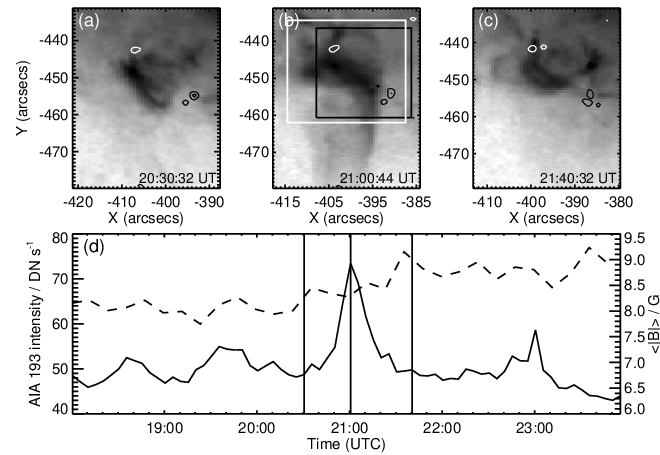
With regard to the magnetic structure of the bright point, we first consider the long term evolution as obtained from 12-minute cadence HMI magnetograms and 5-minute cadence A193 images. (The A193 images were again derived by averaging five consecutive 12-second cadence images.) Figure 3a–c shows three A193 images from before, during and after the jet, with the HMI magnetograms over-plotted as contours. These reveal that the bright point had a fairly simple, tilted bipole structure that was largely unchanged by the jet. In particular the strengths of the magnetic poles did not change, nor did they move closer together. (The LOS magnetic field strengths of the negative and positive poles were around and G at the time of the jet.) This contrasts with the 9-Feb jet for which the magnetic poles of the bright point came together and canceled. For a six hour period from 18:00 to 24:00 UT, a A193 light curve for the bright point was created by averaging the signal from a 28 28 box (indicated on Figure 3b), and it is shown in Figure 3d. The basic morphology of the bright point first appeared around 18:40 UT (the first intensity peak in Figure 3d) and remained present until 23:25 UT. There are four main intensity brightenings seen in the light curve, the largest corresponding to the jet discussed in the present work. The brightening at around 19:40 UT also produced a jet, although much smaller and less dynamic than the blowout jet. The evolution of the average, unsigned magnetic flux is shown in Figure 3d as a dashed line. The flux was derived by averaging the absolute flux over a box of size 22 25 (indicated on Figure 3b) that enclosed the two dominant polarities of the bright point. It can be seen that there was relatively little change in the magnetic field, with a slight increase with time. This again contrasts with the 9-Feb jet for which there was a clear decrease in unsigned magnetic flux over a four hour period.
The fact that the loop ejected from the bright point first rose from the negative polarity part of the bright point gives an important clue as to the magnetic evolution that triggered the jet. To investigate further we took the 45-second cadence HMI magnetograms and binned consecutive sets of five images to yield magnetograms at a 225-second cadence. This sequence revealed that a positive polarity feature with a strength of up to 35 G appeared about 5 north of the negative pole at around 20:10 UT, moved toward it, and canceled with it by around 21:30 UT. Four frames from this sequence are shown in Figure 2b. The boxes on these plots show the location where flux cancelation occurred, and the signed flux within these boxes was averaged to yield the average magnetic flux that is shown in Figure 2a. As the weak positive polarity is canceled around 20:54 UT, the average signed flux becomes more negative. As discussed by Young & Muglach (2013), jets are commonly associated with canceling flux. Unlike the 9-Feb jet, however, the dominant magnetic poles of the bright point remained relatively unaffected, explaining why the bright point was not destroyed by the jet in this case. Note that the high spatial resolution magnetograms of HMI are critical to observing the weak positive polarity feature: a lower resolution or lower sensitivity instrument likely would not have captured this.
To summarize the SDO observations, the jet was triggered by magnetic cancellation at one footpoint of the bipole. The jet erupted as an elongated loop-like shape visible only in the A193 and A211 filters, suggesting that the plasma has a temperature of 1.5–2.0 MK. The ejection of chromospheric plasma was implied by the loop appearing in absorption in the A171 channel. The loop was present for about 25 mins before fading down to background levels, and the light curve of the jet in the A193 filter was closely matched to that of the bright point. The loop appeared highly elongated with an aspect ratio up to approximately 4, although this may be a line-of-sight effect. It is not clear if the loop broke open at the apex during the eruption due to the low signal-to-noise at large heights. The projected maximum extent of the loop above the bright point was around 30 Mm.
4 EIS observations
EIS scanned the jet and bright point between 20:56 and 21:03 UT, and there was a strong velocity signal in four consecutive exposures at 20:58, 20:59, 21:00 and 21:01 UT for which the 195.12 line displayed significant emission on the short wavelength side of the line. A 13 81 pixel sub-region around the jet was extracted and the Fe xii 195.12 line was fit with two Gaussians over this region using the IDL routine EIS_AUTO_FIT (Young, 2012). The fit was constrained by requiring that the two Gaussians had the same width, and that the spectrum background near the lines was flat. We refer to the Gaussian component nearest the rest wavelength of the line as the primary component, and the blue-shifted component as the secondary component. Figures 4b and d show intensity maps derived from the primary and secondary components. The rest component looks quite similar to the A193 image (Figure 4a), with a small bright point and weak, loop-like emission extending southwards from the bright point. The intensity image from the secondary component (Figure 4d) has significant intensity from the top of the weak loop, the right-hand side of the loop and a section of the bright point (only the exposure at 20:59 UT, X-pixel 6). Velocity images from the two EIS Fe xii components are shown in Figures 4c and e. The primary component of the line shows significant blueshifts in the expanding loop, with velocities of around to km s-1. The secondary component shows velocities of to km s-1.
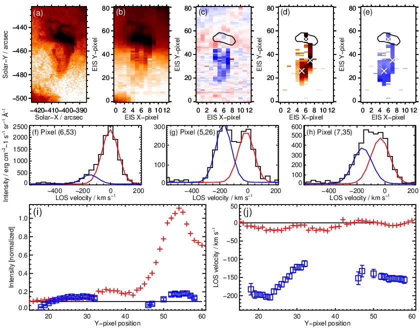
Example line profiles from individual spatial pixels within the jet are shown in Figures 4f, g and h. Figure 4f shows a profile for the jet base where the secondary component is seen as a bump on the side of the dominant primary component. Figure 4g shows an example profile from near the top of the ejected loop where the secondary component is stronger than the primary component, and Figure 4h shows an example where a single broad feature is observed in the leg of the loop. Although two Gaussian components are fit to this feature, it is possible that there is a wide range of velocities that combine to give the observed feature.
Cuts through the EIS intensity and velocity images are shown in Figures 4i and j. X-pixel number 6 was selected, corresponding to a time of 20:59 UT. This exposure shows a significant blue-shifted component in the bright point (see also Figure 4f) as well as the expanding loop. The horizontal line in Figure 4i shows the background coronal hole intensity (note: all intensities have been normalized to the average intensity of the bright point). The expanding loop intensity is only a factor two or less brighter than the background, but because EIS is able to resolve the two velocity components of 195.12 then a faint, highly-blueshifted signal can be detected to large heights. The velocity cross-sections for X-pixel 6 show large velocities in both the bright point and the expanding loop. The primary component of the profile shows blue-shifted velocities of up to 20 km s-1 in the expanding loop.
The LOS velocities of the secondary component from X-pixel 6 are seen to increase away from the bright point between Y-pixels 32 and 23. This behavior suggests that plasma acceleration is occurring within the jet, and it was also seen in the 9-Feb jet (Young & Muglach, 2013) where it was cited as evidence for the nonlinear Alfvén waves predicted from the jet model of Pariat et al. (2009). Although not shown, we note that comparable velocity increases are seen in X-pixels 4 and 5, and a smaller, though still significant, velocity increase is seen from X-pixel 7.
As the jet is spatially resolved in the transverse direction to the jet axis, then it is possible to consider the variation of LOS velocity across the jet. Three-dimensional models of jets (Pariat et al., 2009, e.g.,) predict some degree of twisting motion which would be reflected in the LOS velocities being larger on one side of the jet than the other. Figure 5 shows velocity cross-sections through the jet at three Y-positions (refer to Figure 4e for the locations of the pixels). Although larger velocities are seen on the right-side of the jet (X-pixel 7) compared to the left-side of the jet, consistent with twist, there is not a monotonic variation of LOS velocity across the jet axis. This may indicate more complex motions within the jet, but we also caution that the data points are taken over a period of four minutes and there is likely a significant time dependence that can not be accounted for. Despite this it is clear that the sensitivity of the EIS velocity measurements is sufficient to resolve twisting motions and there is some evidence that the present jet is twisted with the right-side showing a larger LOS speed compared to the left-side by 60 km s-1. This would correspond to anti-clockwise rotation if looking down the axis of the jet towards the bright point.

If we interpret the velocity difference between X-pixels 4 and 7 as representing the rotational motions around the axis of the jet, then we can estimate the angular speed and period as rad s-1 and 690 s, respectively, where is the angle between the jet axis and the LOS to the observer. Given the location on the solar surface of the bright point and the morphology of the images, we consider it likely that –90∘, giving –1.0. The cylindrical radius of the jet is taken to be 4.5= 3300 km based on the width of the EIS velocity feature. Shen et al. (2011) found values of rad s-1 and 564 s for an active region jet, Chen et al. (2012) values of rad s-1 and 452 s for a coronal hole jet, and Hong et al. (2013) values of rad s-1 and 475 s for another coronal hole jet, so the present values are comparable. We note that these authors derived the twist parameters through high-cadence imaging by tracking the transverse motions of discrete structures within the jets.
The temperature reached by the bright point during the event was investigated by creating an average spectrum from the EIS data. Thirty-five spatial pixels in the brightest part of the Fe xii 195.12 image were selected and averaged using the IDL routine EIS_MASK_SPECTRUM (Young, 2012), and Gaussians were fit to the emission lines in the spectrum using the IDL routine SPEC_GAUSS_EIS. The line intensities are given in Table 1. The spectrum showed a weak Fe xv 284.16 line, but Fe xvi 262.99 was not present. The densities derived from the Fe xii 186.88/195.12 and Fe xiii 203.82/202.04 ratios are and 8.86, respectively. We refer the reader to Young et al. (2009) for details on applying these diagnostics to EIS data, and we note that atomic data were taken from version 7.1 of the CHIANTI atomic database (Dere et al., 1997; Landi et al., 2013). Emission lines of Fe viii–xiii and Fe xv are available from the data-set, and the intensities of the lines have been converted to column emission measure values using the method described in Section 3.1 of Tripathi et al. (2010). The emission measure values are plotted in Figure 6. The coronal iron abundance value of Schmelz et al. (2012) was used, and the density was assumed to be constant with temperature with a value of . The emission measure curve peaks at (Fe xi), and falls sharply between Fe xiii and Fe xv. This is consistent with the lack of Fe xvi 262.99 emission, and also the very weak signal in the A335 channel. We can thus place a constraint on the maximum temperature reached in the bright point as (2 MK). Previously Doschek et al. (2010) presented an analysis of a coronal hole bright point that produced a jet and found similar plasma parameters to those found here. No Fe xvi emission was seen, the differential emission measure curve peaked at , and the density (derived from three diagnostics) was –9.05.

For the jet, a block of pixels at the tip of the jet was averaged to yield a single spectrum. Another block of pixels to the right of the jet was also averaged to yield a background spectrum that was subtracted from the jet spectrum, thus isolating the jet emission from the background. This demonstrated that the jet only emits in Fe xi–xiii, with no significant emission from Fe viii–x or Fe xv. The intensities for the Fe xi–xiii lines are shown in Table 1. The density implied from the Fe xii 186.88/195.12 diagnostic is . Isothermal temperatures derived from Fe xii 195.12/Fe xi 188.22 and Fe xiii 202.04/Fe xii 195.12 are and 6.23, respectively. (These values were derived using the CHIANTI atomic database.) The LOS velocities of Fe xi–xiii – measured relative to the line positions in the background spectrum – are , and km s-1 for Fe xi 192.81, Fe xii 195.12 and Fe xiii 202.04, suggesting that there is a temperature dependence of the outflow speed.
| Intensity (erg cm-2 s-1 sr-1) | |||
|---|---|---|---|
| Ion | Line | BP | Jet |
| Fe viii | 185.21 | — | |
| Fe ix | 197.86 | — | |
| Fe x | 184.54 | — | |
| Fe xi | 188.22 | ||
| Fe xii | 195.12 | ||
| 186.88 | |||
| Fe xiii | 202.04 | ||
| 203.82 | — | ||
| Fe xv | 284.16 | — | |
The jet parameters can be compared with previous EIS observations of coronal hole jets studied by Doschek et al. (2010) and Young & Muglach (2013). Doschek et al. (2010) found temperatures of –6.12 using a Fe xi/Fe xii ratio, measured at four heights along their jet. Young & Muglach (2013) used a Fe xi/Fe xii ratio to derive a temperature of . Doschek et al. (2010) measured densities of and 8.85 at two locations in their jet, and Young & Muglach (2013) found a density of . These results suggest that coronal hole jets typically release plasma close to the formation temperature of Fe xi and Fe xii (–6.2) and with a low density typical of coronal hole or quiet Sun plasma.
5 Summary
The key properties of the 8-Feb jet are as follows:
- •
The jet is an expanding, loop-shaped structure that emerges from the negative polarity end of a small magnetic bipole.
- •
The jet is triggered by cancellation of a weak, positive polarity magnetic feature that moves towards the negative pole of the bipole.
- •
The bright point does not get hotter than 2.0 MK during the event, and the coronal density is cm-3.
- •
The jet duration is 25 minutes, and the bright point is not significantly disrupted by the jet occurrence (the intensity returns to the pre-jet levels, and the magnetic field strength remains similar).
- •
The jet extends 30 Mm (projected distance) above the bright point and the temperature of the ejected plasma is 1.7 MK; the density is in the range 0.9 to 1.7 cm-3; and absorption in the A171 channel suggests that chromospheric plasma is also ejected.
- •
LOS speeds increase with distance from the bright point, reaching values up to 250 km s-1.
- •
Evidence from the spectroscopic LOS velocities is found for twisted motions in the jet, and an angular speed of rad s-1 is derived.
Comparing with the 9-Feb jet analyzed by Young & Muglach (2013), the key difference lies with the magnetic field evolution: for the 9-Feb jet the two dominant polarities canceled with each other, whereas for the 8-Feb jet a parasitic polarity emerges near the negative polarity footpoint, and cancels with it. This difference is reflected in the evolution of the bright point during the event: the base arch of the 9-Feb jet is blown open by the jet, and a number of very intense kernels are seen; yet for the 8-Feb jet the base arch remains and no kernels were seen. Despite these differences, the temperature, density and velocity of the ejected plasma are similar between the two events.
On-disk observations of coronal holes afford an excellent opportunity for comparing different types of coronal jet, as both the magnetic and coronal evolution can be studied. The results here and in Young & Muglach (2013) suggest that blowout jets can behave quite differently depending on the particular magnetic field geometry and evolution. Further categorization perhaps based on the types of magnetic field interaction (majority–majority or minority–majority cancelation) may be appropriate.
The authors acknowledge funding from National Science Foundation grant AGS-1159353, and we thank the referee for valuable comments. P.R.Y. thanks ISSI for financial support to attend the 2014 International Team Meeting “Understanding Solar Jets and their Role in Atmospheric Structure and Dynamics” (PI: N.-E. Raouafi), and he thanks the participants for useful discussions. Hinode is a Japanese mission developed and launched by ISAS/JAXA, with NAOJ as domestic partner and NASA and STFC (UK) as international partners. It is operated by these agencies in co-operation with ESA and NSC (Norway). SDO is a mission for NASA’s Living With a Star program, and data are provided courtesy of NASA/SDO and the AIA and HMI science teams.
References
- Chen et al. (2012) Chen, H.-D., Zhang, J., & Ma, S.-L. 2012, Research in Astronomy and Astrophysics, 12, 573
- Dere et al. (1997) Dere, K. P., Landi, E., Mason, H. E., Monsignori Fossi, B. C., & Young, P. R. 1997, A&AS, 125, 149
- Doschek et al. (2010) Doschek, G. A., Landi, E., Warren, H. P., & Harra, L. K. 2010, ApJ, 710, 1806
- Hong et al. (2011) Hong, J., Jiang, Y., Zheng, R., Yang, J., Bi, Y., & Yang, B. 2011, ApJ, 738, L20
- Hong et al. (2013) Hong, J.-C., Jiang, Y.-C., Yang, J.-Y., Zheng, R.-S., Bi, Y., Li, H.-D., Yang, B., & Yang, D. 2013, Research in Astronomy and Astrophysics, 13, 253
- Landi et al. (2013) Landi, E., Young, P. R., Dere, K. P., Del Zanna, G., & Mason, H. E. 2013, ApJ, 763, 86
- Lee et al. (2013) Lee, K.-S., Innes, D. E., Moon, Y.-J., Shibata, K., Lee, J.-Y., & Park, Y.-D. 2013, ApJ, 766, 1
- Liu et al. (2011) Liu, C., Deng, N., Liu, R., Ugarte-Urra, I., Wang, S., & Wang, H. 2011, ApJ, 735, L18
- Moore et al. (2010) Moore, R. L., Cirtain, J. W., Sterling, A. C., & Falconer, D. A. 2010, ApJ, 720, 757
- Moore et al. (2013) Moore, R. L., Sterling, A. C., Falconer, D. A., & Robe, D. 2013, ApJ, 769, 134
- Nisticò et al. (2009) Nisticò, G., Bothmer, V., Patsourakos, S., & Zimbardo, G. 2009, Sol. Phys., 259, 87
- O’Dwyer et al. (2010) O’Dwyer, B., Del Zanna, G., Mason, H. E., Weber, M. A., & Tripathi, D. 2010, A&A, 521, A21
- Pariat et al. (2009) Pariat, E., Antiochos, S. K., & DeVore, C. R. 2009, ApJ, 691, 61
- Schmelz et al. (2012) Schmelz, J. T., Reames, D. V., von Steiger, R., & Basu, S. 2012, ApJ, 755, 33
- Schmieder et al. (2013) Schmieder, B., et al. 2013, A&A, 559, A1
- Shen et al. (2012) Shen, Y., Liu, Y., Su, J., & Deng, Y. 2012, ApJ, 745, 164
- Shen et al. (2011) Shen, Y., Liu, Y., Su, J., & Ibrahim, A. 2011, ApJ, 735, L43
- Shibata & Uchida (1986) Shibata, K., & Uchida, Y. 1986, Sol. Phys., 103, 299
- Shimojo et al. (1996) Shimojo, M., Hashimoto, S., Shibata, K., Hirayama, T., Hudson, H. S., & Acton, L. W. 1996, PASJ, 48, 123
- Tripathi et al. (2010) Tripathi, D., Mason, H. E., Del Zanna, G., & Young, P. R. 2010, A&A, 518, A42
- Young & Muglach (2013) Young, P., & Muglach, K. 2013, ArXiv e-prints
- Young (2012) Young, P. R. 2012, EIS Software Note No. 16, ver. 2.4
- Young et al. (2009) Young, P. R., Watanabe, T., Hara, H., & Mariska, J. T. 2009, A&A, 495, 587