IPMU14-0007

Electroweak baryogenesis in the MSSM with vector-like superfields

Xue Chang, Ran Huo Affiliation: State Key Laboratory of Theoretical Physics, Institute of Theoretical Physics, Chinese Academy of Sciences, P.O. Box 2735, Beijing 100190, China
Kavli IPMU (WPI), The University of Tokyo, 5-1-5 Kashiwanoha, Kashiwa, CHiba 277-8583, Japan Email: chxue@itp.ac.cn, ran.huo@ipmu.jp

Abstract

Introducing heavy particles with strong couplings to the Higgs field can strengthen electroweak phase transition, through the entropy release mechanism from both bosons and fermions. We analyze the possibility of electroweak baryogenesis in the MSSM with new vector-like superfields. The new vector-like particles belong to the representation $5+\overline{5}+10+\overline{10}$ of $SU(5)$ . By analyzing in detail the effective potential at finite temperature, we show that a strongly first order electroweak phase transition in this model is ruled out by a combination of 125 GeV Higgs requirement, the bound for exotic quarks, the gluon fusion Higgs production rate and the Higgs diphoton decay rate as well as the electroweak precision measurement.

Keywords:

supersymmetry,

pacs

11.10.Wx, 12.10.-g, 11.30.Pb

I Introduction

The origin of the matter anti-matter asymmetry of our universe remains unclear. The three Sakharov conditions [1] can be fulfilled in high scale mechanisms such as leptogenesis [2, 3] and Grand Unified Theory (GUT) baryogenesis [4, 5, 6, 7], but are difficult to test by electroweak (EW) scale experiments. While electroweak baryogenesis (EWBG) [8], relying on weak scale physics, provides an alternative solution which requires a strongly first-order phase transition (SFOPT) [9]. Unfortunately, the EW phase transition (EWPT) is too weak in the Standard Model (SM) with large Higgs mass [10, 11] and the CP violation is too small [12].

Extensions of the SM with new EW scale physics can lead to a SFOPT, in all of which new particles beyond the SM are needed. On the other hand, the ATLAS and CMS collaborations at the CERN Large Hadron Collider (LHC) reported observation of a SM-like Higgs boson with mass of $125-126$ GeV [13, 14]. If we require the EWBG mechanism to account for the matter anti-matter asymmetry, the new fields introduced for a SFOPT can induce significant corrections to the SM-like Higgs mass as well as production and decay rates, which will be strongly constrained. For example in the Minimal Supersymmetric Standard Model (MSSM), the light stop scenario [15, 16] has been severely constrained [17].

Based on what physics is responsible for generating the barrier between the symmetric and broken phases, there are three EWPT model classes in general [18]. In this paper, we focus on the thermally driven case. In addition to the effect induced by terms cubic in $\phi$ in the bosonic high temperature expansion, the phase transition can be strengthened by introducing heavy particles with strong couplings to the Higgs fields, such as the SM extension with TeV Higgsinos, Winos and Binos [19, 20]. That is, after the electroweak symmetry breaking (EWSB), the new particles get Yukawa masses and become heavier, they approximately decouple from the thermal plasma and transfer their entropy into the thermal bath. In this paper we consider a different model, namely in addition to the MSSM, adding several vector-like (VL) superfields. This kind of model [22, 23] have been extensively studied and found interesting, for it can relax the naturalness problem raised by the Higgs mass, be consistent with gauge coupling unification and precision EW measurements, and have a rich phenomenology. So it is interesting to explore its possibility to realize the SFOPT in detail.

The added exotic particles belong to the representation $5+\overline{5}+10+\overline{10}$ of $SU(5)$ , which consists four new quarks, two new charged leptons, two left handed neutrinos and the corresponding sparticles with total degree of freedom 120. The model is the MSSM with two new supersymmetric generations, while VL mass terms are introduced between the two to escape the experimental 4th generation search bound. In search for a SFOPT we analyze in details the zero temperature potential, the one-loop zero temperature potential and the finite temperature potential. To search for viable parameter region we also impose all conventional constraints: the SM like Higgs mass is about $125$ GeV, no new light quarks of a few hundred GeV exist [24], the gluon fusion Higgs production rate and the Higgs diphoton decay rate are not significantly changed [13, 14], and the Peskin-Takeuchi parameters $T$ and $S$ [25] are small.

We find generally a SFOPT combining with a 125 GeV Higgs requirement will lead to a too light exotic fermion/scalar. In order to make them heavy enough to escape the direct search bound the VL masses should be about $500$ GeV, but the VL Yukawa are also pushed to large values near the perturbativity bound. We find an almost supersymmetric VL sector with large $\tan\beta$ and no scalar mixing as our best solution, which can satisfy the $125$ GeV Higgs requirement without changing the Higgs gluon fusion rate and the Higgs diphoton decay rate. However, it is still in tension with the direct light new particle search, and eventually ruled out by contributing a very large Peskin-Takeuchi $T$ parameter. So in all, the possibility of EWBG induced by supersymmetric VL generations in our setup is fairly ruled out.

The outline of the rest of the paper is as follows: We will define the model precisely in section II. In section III and IV we investigate the zero temperature potential (as well as the Higgs mass) and the finite temperature potential separately. Section V contains our final results and discussions of various constraints. A brief summary is given in the last section.

II The MSSM with Vector-Like Superfields

As mentioned above, new particles beyond the MSSM are two new generations $5+\overline{5}+10+\overline{10}$ of $SU(5)$ . Here we do not take the singlet right hand neutrino into account, so there will be no Yukawa couplings of the VL neutrinos and the neutrinos do not contribute to EWSB. Moreover, the model almost preserve gauge couplings unification [27], so it is also UV motivated.

The corresponding quantum numbers of VL superfields under SU(3) ${}_{c}\times$ SU(2) ${}_{L}\times$ U(1)_Y are given as

\begin{array}[]{c}Q(3,2,\frac{1}{3}),~~~~~U(3,1,\frac{4}{3}),~~~~D(3,1,-\frac{2}{3}),~~~L(1,2,-1),~~~E(1,1,-2),\\ \overline{Q}(\bar{3},2,-\frac{1}{3}),~~~~\overline{U}(\bar{3},1,-\frac{4}{3}),~~~~\overline{D}(\bar{3},1,\frac{2}{3}),~~~~\overline{L}(1,2,1),~~~~\overline{E}(1,1,2).\end{array}

(1)

And the superpotential is

\begin{array}[]{lll}W&=&W_{\mathrm{MSSM}}+M_{Q}\overline{Q}Q+M_{U}\overline{U}U+M_{D}\overline{D}D+M_{L}\overline{L}L+M_{E}\overline{E}E\\ &&+k_{1}H_{u}Q\overline{U}+k_{2}H_{u}\overline{Q}D+k_{3}H_{u}\overline{L}E-k_{1}^{{}^{\prime}}H_{d}\overline{Q}U-k_{2}^{{}^{\prime}}H_{d}Q\overline{D}-k_{3}^{{}^{\prime}}H_{d}L\overline{E}~.\end{array}

(2)

Note that in general there are mixing between the new vector-like superfields and the MSSM superfields. The related Yukawa couplings with the first/second family MSSM fields are strongly constrained by the EW phenomenology such as flavor changing neutral current [26], which need to be less than $10^{-3}$ . The constraint on the couplings with the third family MSSM fields is relatively loose, which can be of order $0.1$ . We ignore the effect of these terms just in the EWPT calculation for simplicity.

By assuming universality of the mass-squared terms and the alignment of the B terms, the soft mass terms and the trilinear soft terms of all the VL scalar partners are given by

$\displaystyle-{\mathcal{L}}_{\mathrm{soft}}$	$\displaystyle=$	$\displaystyle m^{2}_{Q}\|\tilde{Q}\|^{2}+m^{2}_{\bar{Q}}\|\tilde{\bar{Q}}\|^{2}+m^{2}_{U}\|\tilde{U}\|^{2}+m^{2}_{\bar{U}}\|\tilde{\bar{U}}\|^{2}+m^{2}_{D}\|\tilde{D}\|^{2}+m^{2}_{\bar{D}}\|\tilde{\bar{D}}\|^{2}$	(3)
		$\displaystyle+m^{2}_{L}\|\tilde{L}\|^{2}+m^{2}_{\bar{L}}\|\tilde{\bar{L}}\|^{2}+m^{2}_{E}\|\tilde{E}\|^{2}+m^{2}_{\bar{E}}\|\tilde{\bar{E}}\|^{2}+(B_{Q}M_{Q}\tilde{Q}\tilde{\bar{Q}}+B_{U}M_{U}\tilde{U}\tilde{\bar{U}}$
		$\displaystyle+B_{D}M_{D}\tilde{D}\tilde{\bar{D}}+B_{L}M_{L}\tilde{L}\tilde{\bar{L}}+B_{E}M_{E}\tilde{E}\tilde{\bar{E}}+A_{k_{t}}k_{1}H_{u}\tilde{Q}\tilde{\bar{U}}+A_{k_{b}}k_{2}H_{u}\tilde{\bar{Q}}\tilde{D}$
		$\displaystyle-A_{k_{t}^{{}^{\prime}}}k_{1}^{{}^{\prime}}H_{d}\tilde{\bar{Q}}\tilde{U}-A_{k_{b}^{{}^{\prime}}}k_{2}^{{}^{\prime}}H_{d}\tilde{Q}\tilde{\bar{D}}-A_{k_{\tau}^{{}^{\prime}}}k_{3}^{{}^{\prime}}H_{d}\tilde{L}\tilde{\bar{E}}+\mathrm{c.c.}).$

From Eq. (2, 3), the new charged fermions field-dependent mass matrices are

{\mathcal{M}}_{U}(\phi)=\begin{pmatrix}M_{Q}&k_{1}\frac{\phi_{u}}{\sqrt{2}}\\ k_{1}^{{}^{\prime}}\frac{\phi_{d}}{\sqrt{2}}&M_{U}\\ \end{pmatrix}~,~{\mathcal{M}}_{D}(\phi)=\begin{pmatrix}M_{Q}&k_{2}^{{}^{\prime}}\frac{\phi_{d}}{\sqrt{2}}\\ k_{2}\frac{\phi_{u}}{\sqrt{2}}&M_{D}\\ \end{pmatrix}~,~{\mathcal{M}}_{E}(\phi)=\begin{pmatrix}M_{L}&k_{3}^{{}^{\prime}}\frac{\phi_{d}}{\sqrt{2}}\\ k_{3}\frac{\phi_{u}}{\sqrt{2}}&M_{E}\\ \end{pmatrix}.

(4)

We have defined¹¹ 1 In this paper we use $s_{\beta},c_{\beta}$ for $\sin\beta,\cos\beta$ $\langle\phi_{d}\rangle=v_{d}=c_{\beta}v$ and $\langle\phi_{u}\rangle=v_{u}=s_{\beta}v$ and $v\simeq 246$ GeV. The corresponding field-dependent sfermion squared-mass matrix, for new up type squark for instance, is

\mathcal{M}^{2}_{\tilde{U}}=\begin{pmatrix}m_{\tilde{{t}}_{L^{{}^{\prime}}}}^{2}&m_{X_{t^{{}^{\prime}}}}^{2}&B_{Q}M_{Q}&M^{*}_{Q}k_{1}\frac{\phi_{u}}{\sqrt{2}}+M_{U}k^{\prime}_{1}\frac{\phi_{d}}{\sqrt{2}}\\ m_{X_{t^{{}^{\prime}}}}^{2}&m_{\tilde{{t}}_{R^{{}^{\prime}}}}^{2}&M_{U}k_{1}\frac{\phi_{u}}{\sqrt{2}}+M^{*}_{Q}k^{\prime}_{1}\frac{\phi_{d}}{\sqrt{2}}&B_{U}M_{U}\\ B_{Q}M_{Q}&M_{U}k_{1}\frac{\phi_{u}}{\sqrt{2}}+M^{*}_{Q}k^{\prime}_{1}\frac{\phi_{d}}{\sqrt{2}}&m_{\tilde{{t}}_{L^{{}^{\prime\prime}}}}^{2}&m_{X_{t^{{}^{\prime\prime}}}}^{2}\\ M^{*}_{Q}k_{1}\frac{\phi_{u}}{\sqrt{2}}+M_{U}k^{\prime}_{1}\frac{\phi_{d}}{\sqrt{2}}&B_{U}M_{U}&m_{X_{t^{{}^{\prime\prime}}}}^{2}&m_{\tilde{{t}}_{R^{{}^{\prime\prime}}}}^{2}\end{pmatrix},

(5)

in which the basis is $(\bar{Q}^{*},U,Q,\bar{U}^{*})$ , and we have defined

\begin{array}[]{lll}m_{\tilde{t}_{L^{\prime}}}^{2}(\phi)=M_{Q}^{2}+m_{\bar{Q}}^{2}+\frac{1}{2}k_{1}^{{}^{\prime}2}\phi_{d}^{2}+D_{\tilde{t}_{L^{\prime}}}^{2}(\phi)\\ m_{\tilde{t}_{R^{\prime}}}^{2}(\phi)=M_{U}^{2}+m_{U}^{2}+\frac{1}{2}k_{1}^{{}^{\prime}2}\phi_{d}^{2}+D_{\tilde{t}_{R^{\prime}}}^{2}(\phi)\\ m_{\tilde{t}_{L^{\prime\prime}}}^{2}(\phi)=M_{Q}^{2}+m_{Q}^{2}+\frac{1}{2}k_{1}^{2}\phi_{u}^{2}+D_{\tilde{t}_{L^{\prime\prime}}}^{2}(\phi)\\ m_{\tilde{t}_{R^{\prime\prime}}}^{2}(\phi)=M_{U}^{2}+m_{\bar{U}}^{2}+\frac{1}{2}k_{1}^{2}\phi_{u}^{2}+D_{\tilde{t}_{R^{\prime\prime}}}^{2}(\phi)\\ m_{X_{t^{\prime}}}^{2}(\phi)=k_{1}^{{}^{\prime}}(A_{k_{t^{\prime}}}\frac{\phi_{d}}{\sqrt{2}}-\mu\frac{\phi_{u}}{\sqrt{2}})\\ m_{X_{t^{\prime\prime}}}^{2}(\phi)=k_{1}(A_{k_{t}}\frac{\phi_{u}}{\sqrt{2}}-\mu\frac{\phi_{d}}{\sqrt{2}})\\ D_{\tilde{t}_{L^{\prime}}}^{2}(\phi)=-D_{\tilde{t}_{L^{\prime\prime}}}^{2}(\phi)=-(\frac{g^{2}}{8}-\frac{g^{\prime 2}}{12})(\phi_{d}^{2}-\phi_{u}^{2}),\\ D_{\tilde{t}_{R^{\prime}}}^{2}(\phi)=-D_{\tilde{t}_{R^{\prime\prime}}}^{2}(\phi)=-\frac{g^{\prime 2}}{6}(\phi_{d}^{2}-\phi_{u}^{2}).\end{array}

(6)

The squared-mass matrices for down type squark and charged slepton are similar. After diagonalization we get two new Dirac up-type quarks $t^{\prime}_{1,2}$ , two new Dirac down-type quarks $b^{\prime}_{1,2}$ , two new Dirac charged leptons $\tau^{\prime}_{1,2}$ , and two new left-handed neutrino $\nu^{\prime}_{1,2}$ as well as their superpartners $\tilde{t}^{\prime}_{1,2,3,4}$ , $\tilde{b}^{\prime}_{1,2,3,4}$ , $\tilde{\tau}^{\prime}_{1,2,3,4}$ , and $\tilde{\nu}^{\prime}_{1,2}$ ²² 2 Strictly speaking (s)neutrinos don’t need diagonalization..

In the following calculation we neglect all the D-terms and B-terms in the mass matrices ³³ 3 At phase transition the D-terms are comparable with top squark thermal mass in Eq. (49) which we are not ignoring, but here we have more important contribution from VL Yukawa couplings in any way.. For simplicity we further assume at low scale (namely without renormalization group equation (RGE) running):

$\displaystyle m^{2}_{Q}=m^{2}_{\bar{Q}}=m^{2}_{U}=m^{2}_{\bar{U}}=m^{2}_{D}=m^{2}_{\bar{D}}=m^{2}_{L}=m^{2}_{\bar{L}}=m^{2}_{E}=m^{2}_{\bar{E}}$	$\displaystyle=$	$\displaystyle m^{2},$
$\displaystyle M_{Q}=M_{U}=M_{D}=M_{L}=M_{E}$	$\displaystyle=$	$\displaystyle M_{V},$
$\displaystyle A_{k_{t,b,\tau}}=A_{k_{t^{\prime},b^{\prime},\tau^{\prime}}}$	$\displaystyle=$	$\displaystyle A,$	(7)

and define the VL scalar squared-mass average and the mass mixing parameter as

$\displaystyle M^{2}_{S}$	$\displaystyle=$	$\displaystyle M^{2}_{V}+m^{2},$
$\displaystyle X_{1}$	$\displaystyle=$	$\displaystyle A-\mu\mathrm{cot}\beta,$
$\displaystyle X_{2}$	$\displaystyle=$	$\displaystyle A-\mu\mathrm{tan}\beta.$	(8)

We choose $\tan\beta=10$ as our benchmark. Note that the Yukawa $k_{1,2,3}$ are always combined with $\phi_{u}$ and the Yukawa $k^{\prime}_{1,2,3}$ with $\phi_{d}$ , the latter is always suppressed by $\tan\beta$ . We actually set $k^{\prime}_{1,2,3}$ to zero (see the discussion of the gluon fusion and Higgs diphoton deacy), then $\phi_{d}$ decouples. Arising from the first mass matrix in Eq. (4), the field-dependent squared-mass eigenvalues of $t^{{}^{\prime}}_{1,2}$ can be simplified as

\displaystyle m_{{t^{{}^{\prime}}_{1,2}}}^{2}(\phi_{u},\phi_{d})

\displaystyle=

\displaystyle M^{2}_{V}+\frac{1}{4}k^{2}_{1}\phi^{2}_{u}\mp\frac{1}{4}\sqrt{k^{4}_{1}\phi^{4}_{u}+8M^{2}_{V}k^{2}_{1}\phi^{2}_{u}}~,

(9)

and the four field-dependent squared-mass eigenvalues, arising from Eq. (5,6), are

$\displaystyle m_{{\tilde{t}^{{}^{\prime}}_{1}}}^{2}(\phi_{u},\phi_{d})$	$\displaystyle=$	$\displaystyle M^{2}_{S}+\frac{1}{4}k^{2}_{1}\phi^{2}_{u}-\frac{1}{2\sqrt{2}}k_{1}\phi_{u}X_{1}$	(10)
		$\displaystyle-\frac{1}{2}\sqrt{(\frac{1}{2}k^{2}_{1}\phi^{2}_{u}-\frac{1}{\sqrt{2}}k_{1}\phi_{u}X_{1})^{2}+2M^{2}_{V}k^{2}_{1}\phi^{2}_{u}},$	(10)
$\displaystyle m_{{\tilde{t}^{{}^{\prime}}_{2}}}^{2}(\phi_{u},\phi_{d})$	$\displaystyle=$	$\displaystyle M^{2}_{S}+\frac{1}{4}k^{2}_{1}\phi^{2}_{u}+\frac{1}{2\sqrt{2}}k_{1}\phi_{u}X_{1}$	(11)
		$\displaystyle-\frac{1}{2}\sqrt{(\frac{1}{2}k^{2}_{1}\phi^{2}_{u}+\frac{1}{\sqrt{2}}k_{1}\phi_{u}X_{1})^{2}+2M^{2}_{V}k^{2}_{1}\phi^{2}_{u}},$	(11)
$\displaystyle m_{{\tilde{t}^{{}^{\prime}}_{3}}}^{2}(\phi_{u},\phi_{d})$	$\displaystyle=$	$\displaystyle M^{2}_{S}+\frac{1}{4}k^{2}_{1}\phi^{2}_{u}-\frac{1}{2\sqrt{2}}k_{1}\phi_{u}X_{1}$	(12)
		$\displaystyle+\frac{1}{2}\sqrt{(\frac{1}{2}k^{2}_{1}\phi^{2}_{u}-\frac{1}{\sqrt{2}}k_{1}\phi_{u}X_{1})^{2}+2M^{2}_{V}k^{2}_{1}\phi^{2}_{u}},$	(12)
$\displaystyle m_{{\tilde{t}^{{}^{\prime}}_{4}}}^{2}(\phi_{u},\phi_{d})$	$\displaystyle=$	$\displaystyle M^{2}_{S}+\frac{1}{4}k^{2}_{1}\phi^{2}_{u}+\frac{1}{2\sqrt{2}}k_{1}\phi_{u}X_{1}$	(13)
		$\displaystyle+\frac{1}{2}\sqrt{(\frac{1}{2}k^{2}_{1}\phi^{2}_{u}+\frac{1}{\sqrt{2}}k_{1}\phi_{u}X_{1})^{2}+2M^{2}_{V}k^{2}_{1}\phi^{2}_{u}}.$	(13)

For field-dependent masses of new down-type quarks, new charged leptons and their superpartners, one just need to substitute $k_{1}\rightarrow k_{2},k_{3}$ .

At the end of this section, we give the direct search limits on new particles. As mentioned before, the exotic heavy fermions can decay into SM particles when kinematically allowed through the mixing Yukawa couplings [22, 23]. Direct searches set limits to the exotic fermions in such decay modes. Limits on sparticles depend on the mixing angles of the mass eigenstates and the mass splittings between them and the lightest neutralino. The strongest current limits on the extra quarks, leptons and their scalar particles are given as [24]

	$\displaystyle m_{t^{\prime}}>685\mathrm{GeV}~,~m_{\tilde{t}^{\prime}}>95.7\mathrm{GeV},$		(14)
	$\displaystyle m_{b^{\prime}}>685\mathrm{GeV}~,~m_{\tilde{b}^{\prime}}>89\mathrm{GeV},$		(15)
	$\displaystyle m_{\tau^{\prime}}>100.8\mathrm{GeV}~,~m_{\tilde{\tau}^{\prime}}>81.9\mathrm{GeV},$		(16)
	$\displaystyle m_{\nu^{\prime}}>39.5\mathrm{GeV}~,~m_{\tilde{\nu}^{\prime}}>94\mathrm{GeV}.$		(17)

However when considering various combinations of decay modes of new fermions and not being limited to a special mass constrain for scalars, the above bounds are relaxed. We will see later that the mass of charged exotic fermions is important to an acceptable SFOPT, so here in our work we consider some optimistic mass limits for new charged fermions. Namely we consider $m_{t^{\prime}}>415\mathrm{GeV}$ for $t^{\prime}$ [29], which is achieved by scanning the exotic decay branching ratio triangle, and $m_{b^{\prime}}>360\mathrm{GeV}$ [22] for $b^{\prime}$ and $m_{\tau^{\prime}}>63.5\mathrm{GeV}$ [30] for $\tau^{\prime}$ . The mass limits for other new particles still take the values shown above.

III Zero Temperature Potential and Higgs Mass

In this model, the zero temperature effective potential at one-loop level are given by

\displaystyle V(\phi_{u},\phi_{d},T=0)

\displaystyle=

\displaystyle V_{0}(\phi_{u},\phi_{d})+V_{1}(\phi_{u},\phi_{d})

(18)

in which $V_{0}$ is the tree-level potential, $V_{1}$ is the zero-temperature renormalized one-loop potential.

III.1 Tree Level Potential

The zero temperature tree-level potential here in our model is the same as in the MSSM, which is given as

\displaystyle V_{\mathrm{MSSM}}

\displaystyle=

\displaystyle\frac{1}{2}m^{2}_{11}\phi_{d}^{2}+\frac{1}{2}m^{2}_{22}\phi_{u}^{2}-m^{2}_{12}\phi_{d}\phi_{u}+\frac{1}{4}\lambda_{1}\phi_{d}^{4}+\frac{1}{4}\lambda_{2}\phi_{u}^{4}+\frac{1}{2}\lambda_{3}\phi_{d}^{2}\phi_{u}^{2},

(19)

in which

$\displaystyle m^{2}_{11}$	$\displaystyle=$	$\displaystyle m^{2}_{H_{d}}+\mu^{2},$	(20)
$\displaystyle m^{2}_{22}$	$\displaystyle=$	$\displaystyle m^{2}_{H_{u}}+\mu^{2},$	(21)
$\displaystyle m^{2}_{12}$	$\displaystyle=$	$\displaystyle b\mu,$	(22)
$\displaystyle\lambda_{1}$	$\displaystyle=$	$\displaystyle\lambda_{2}=-\lambda_{3}=\frac{1}{8}(g^{2}+g^{\prime 2}).$	(23)

III.2 The Renormalization Group Improved Higgs Potential and the SM-Like Higgs Mass

The third generation MSSM particles and the new VL particles will induce significant corrections to the Higgs potential. Here we are interested in the complete one loop improved Higgs potential, because it determines the SM like Higgs mass. We follow [28] to write it as

$\displaystyle V_{\mathrm{MSSM}}$	$\displaystyle=$	$\displaystyle\frac{1}{2}(m^{2}_{11}+\Delta m^{2}_{11})\phi_{d}^{2}+\frac{1}{2}(m^{2}_{22}+\Delta m^{2}_{22})\phi_{u}^{2}-(m^{2}_{12}+\Delta m^{2}_{12})\phi_{d}\phi_{u}$	(24)
		$\displaystyle+\frac{1}{4}(\lambda_{1}+\Delta\lambda_{1})\phi_{d}^{4}+\frac{1}{4}(\lambda_{2}+\Delta\lambda_{2})\phi_{u}^{4}+\frac{1}{2}(\lambda_{3}+\Delta\lambda_{3})\phi_{d}^{2}\phi_{u}^{2}$
		$\displaystyle+\Delta\lambda_{6}\phi_{d}^{3}\phi_{u}+\Delta\lambda_{7}\phi_{d}\phi_{u}^{3},$

where $\Delta\lambda_{6}\phi_{d}^{3}\phi_{u}$ and $\Delta\lambda_{7}\phi_{d}\phi_{u}^{3}$ are the one-loop potential induced terms which don’t exist in the tree-level potential. The expressions for the corrections are listed in Appendix A.

With the renormalization group (RG) improved Higgs potential, the SM-like Higgs mass can be written as

	$\displaystyle m^{2}_{h_{0}}$	$\displaystyle=$	$\displaystyle m^{2}_{Z}\cos^{2}2\beta+2\Delta\lambda_{1}v^{2}\sin^{4}\beta+2\Delta\lambda_{2}v^{2}\cos^{4}\beta+4\Delta\lambda_{3}v^{2}\sin^{2}\beta\cos^{2}\beta$		(25)
			$\displaystyle+8\Delta\lambda_{6}v^{2}\sin\beta\cos^{3}\beta+8\Delta\lambda_{7}v^{2}\sin^{3}\beta\cos\beta.$		(25)

In order to get a simple analytical expression, we set the parameters as mentioned before and further set

\displaystyle k_{1}=k_{2}=k_{3}=k~,~

(26)

then the SM-like Higgs mass can be simplified as

	$\displaystyle m^{2}_{h_{0}}$	$\displaystyle=$	$\displaystyle m^{2}_{Z}\cos^{2}2\beta+\frac{3v^{2}}{4\pi^{2}}y_{t}^{4}[\mathrm{ln}\Big(\frac{\tilde{m}_{t}}{m_{t}}\Big)+\frac{X^{2}_{t}}{2\tilde{m}^{2}_{t}}\Big(1-\frac{X^{2}_{t}}{12\tilde{m}^{2}_{t}}\Big)]$		(27)
			$\displaystyle+\frac{7v^{2}}{8\pi^{2}}k^{4}s^{4}_{\beta}\Bigl[\mathrm{ln}\frac{M^{2}_{S}}{M^{2}_{V}}-\frac{1}{6}\Big(5-\frac{M^{2}_{V}}{M^{2}_{S}}\Big)\Big(1-\frac{M^{2}_{V}}{M^{2}_{S}}\Big)+\hat{X}^{2}_{1}\Big(1-\frac{M^{2}_{V}}{3M^{2}_{S}}\Big)-\frac{\hat{X}^{4}_{1}}{12}\Bigr].$		(27)

We can see that new heavy particles give extra contributions and permitting relatively lighter stop mass, which can loose the tension of the naturalness problem.

III.3 Zero Temperature One-loop Level Potential

In the above analysis we actually run the RGE top down from the supersymmetry breaking scale, in order to fix the low energy Higgs mass to be the observed value. However, as we go to higher scales where the EW phase transition takes place, the RGE running is backwards from the low energy potential Eq. (24). We describe this process in the way of (zero temperature) one loop potential, which is equivalent to RGE⁴⁴ 4 We choose to present the one-loop issue in this awkward way because this is the way we do the numerical work: the Coleman-Weinberg form one loop potential are always implemented by a build-in function in the code CosmoTransition [32], so the low scale parameters consistent with Higgs mass and VEV need to be run down from the supersymmetry breaking scale at first.. The zero-temperature one-loop potential are given by

\displaystyle V_{1}(\phi_{u},\phi_{d})=\frac{1}{64\pi^{2}}\sum_{i}n_{i}m^{4}_{i}(\phi_{u},\phi_{d})\left[~\mathrm{log}\frac{m^{2}_{i}(\phi_{u},\phi_{d})}{Q^{2}}-c_{i}~\right]

(28)

where $m_{i}(\phi_{u},\phi_{d})$ are the field-dependent masses and $Q$ is the renormalization scale⁵⁵ 5 A variation of $Q$ induces variation of $\phi^{2}$ and $\phi^{4}$ terms, in Eq. (29-31) we see that the combination of them together with counterterms are determined by the renormalization condition, so the value of $Q$ is immaterial.. $i$ stands for the particles which can contribute to the effective potential, $n_{i}$ is the particle degree of freedom, $c_{i}$ ’s are constants which are 5/6 for gauge bosons and 3/2 for fermions and scalars. In our work we include the large one-loop corrections induced by top, stop and all the vector-like particles as well as the EW gauge bosons, the corresponding degree of freedoms are: $n_{t}=n_{t^{\prime}_{1,2}}=n_{b^{\prime}_{1,2}}=3n_{\tau^{\prime}_{1,2}}=-12$ , $n_{\tilde{t}_{1,2}}=n_{\tilde{t}^{\prime}_{1,2,3,4}}=n_{\tilde{b}^{\prime}_{1,2,3,4}}=3n_{\tilde{\tau}^{\prime}_{1,2,3,4}}=6$ , $n_{W_{L}}=2$ , $n_{W_{T}}=4$ , $n_{Z_{L}}=1$ , $n_{Z_{T}}=2$ , where subscripts L and T means longitudinal and transverse modes respectively.

As stressed above, the one-loop potential should be renormalized in a way which preserves the low energy Higgs VEV and the Higgs mass. In the one loop potential language it is easy to implement, namely by requiring

\displaystyle\left(\frac{\partial}{\partial\phi_{u}},\frac{\partial}{\partial\phi_{d}},\frac{\partial^{2}}{\partial\phi_{u}^{2}},\frac{\partial^{2}}{\partial\phi_{d}^{2}},\frac{\partial^{2}}{\partial\phi_{u}\partial\phi_{d}}\right)\big(V_{1}(\phi_{u},\phi_{d})+V_{1}^{\mathrm{c.t.}}(\phi_{u},\phi_{d})\big)\bigg|_{\phi_{d}=v_{d},\phi_{u}=v_{u}}=0.

(29)

Here we introduce the finite “counterterms” $V_{1}^{\mathrm{c.t.}}$ to protect the one-loop potential from shifting the Higgs VEV and CP even Higgs mass matrix. We have five equations so that we can determine up to five coefficients of the counterterm polynomial, here we choose them to be

\displaystyle V_{1}^{\mathrm{c.t.}}=\frac{1}{2}\delta m^{2}_{11}\phi_{d}^{2}+\frac{1}{2}\delta m^{2}_{22}\phi_{u}^{2}+\frac{1}{4}\delta\lambda_{1}\phi_{d}^{4}+\frac{1}{4}\delta\lambda_{2}\phi_{u}^{4}+\frac{1}{2}\delta\lambda_{3}\phi_{d}^{2}\phi_{u}^{2}.

(30)

And the corresponding total zero temperature one-loop potential is

			$\displaystyle V_{1}^{\mathrm{re}}(\phi_{u},\phi_{d})_{i}=V_{1}(\phi_{u},\phi_{d})_{i}+V_{1}^{\mathrm{c.t.}}(\phi_{u},\phi_{d})_{i}$		(31)
		$\displaystyle=$	$\displaystyle\frac{n_{i}}{64\pi^{2}}\Bigl[m^{4}_{i}(\phi_{u},\phi_{d})\log\frac{m^{2}_{i}(\phi_{u},\phi_{d})}{Q^{2}}+\alpha^{u}_{i}\phi^{2}_{u}+\alpha^{d}_{i}\phi^{2}_{d}+\beta^{u}_{i}\phi^{4}_{u}+\beta^{d}_{i}\phi^{4}_{d}+2\beta^{ud}_{i}\phi^{2}_{u}\phi^{2}_{d}\Bigr]$		(31)

The solution of Eq. (29) is unique, namely

$\displaystyle\alpha^{u}_{i}$	$\displaystyle=$	$\displaystyle(-\frac{3}{2}\frac{\omega_{i}\omega^{u^{\prime}}_{i}}{v_{u}}+\frac{1}{2}\omega_{i}^{u^{\prime}2}+\frac{1}{2}\omega_{i}\omega^{u^{\prime\prime}}_{i})\log\frac{\omega_{i}}{Q^{2}}-\frac{3}{4}\frac{\omega_{i}\omega^{u^{\prime}}_{i}}{v_{u}}+\frac{3}{2}\omega_{i}^{u^{\prime}2}+\frac{1}{2}\omega_{i}\omega^{u^{\prime\prime}}_{i}-\beta^{ud}_{i}v_{d}^{2}$	(32)
$\displaystyle\alpha^{d}_{i}$	$\displaystyle=$	$\displaystyle(-\frac{3}{2}\frac{\omega_{i}\omega^{d^{\prime}}_{i}}{v_{d}}+\frac{1}{2}\omega_{i}^{d^{\prime}2}+\frac{1}{2}\omega_{i}\omega^{d^{\prime\prime}}_{i})\log\frac{\omega_{i}}{Q^{2}}-\frac{3}{4}\frac{\omega_{i}\omega^{d^{\prime}}_{i}}{v_{d}}+\frac{3}{2}\omega_{i}^{d^{\prime}2}+\frac{1}{2}\omega_{i}\omega^{d^{\prime\prime}}_{i}-\beta^{ud}_{i}v_{u}^{2}$	(33)
$\displaystyle\beta^{u}_{i}$	$\displaystyle=$	$\displaystyle\frac{1}{v^{2}_{u}}\bigl[(\frac{1}{4}\frac{\omega_{i}\omega^{u^{\prime}}_{i}}{v_{u}}-\frac{1}{4}\omega_{i}^{u^{\prime}2}-\frac{1}{4}\omega_{i}\omega^{u^{\prime\prime}}_{i})\log\frac{\omega_{i}}{Q^{2}}+\frac{1}{8}\frac{\omega_{i}\omega^{u^{\prime}}_{i}}{v_{u}}-\frac{3}{8}\omega_{i}^{u^{\prime}2}-\frac{1}{8}\omega_{i}\omega^{u^{\prime\prime}}_{i}\bigr]$	(34)
$\displaystyle\beta^{d}_{i}$	$\displaystyle=$	$\displaystyle\frac{1}{v^{2}_{d}}\bigl[(\frac{1}{4}\frac{\omega_{i}\omega^{d^{\prime}}_{i}}{v_{d}}-\frac{1}{4}\omega_{i}^{d^{\prime}2}-\frac{1}{4}\omega_{i}\omega^{d^{\prime\prime}}_{i})\log\frac{\omega_{i}}{Q^{2}}+\frac{1}{8}\frac{\omega_{i}\omega^{d^{\prime}}_{i}}{v_{d}}-\frac{3}{8}\omega_{i}^{d^{\prime}2}-\frac{1}{8}\omega_{i}\omega^{d^{\prime\prime}}_{i}\bigr]$	(35)
$\displaystyle\beta^{ud}_{i}$	$\displaystyle=$	$\displaystyle-(\frac{\omega^{u^{\prime}}_{i}\omega^{d^{\prime}}_{i}+\omega_{i}\omega^{ud^{\prime\prime}}_{i}}{4v_{u}v_{d}})\log\frac{\omega_{i}}{Q^{2}}+\frac{3\omega^{u^{\prime}}_{i}\omega^{d^{\prime}}_{i}+\omega_{i}\omega^{ud^{\prime\prime}}_{i}}{2v_{u}v_{d}}$	(36)

where we define $\omega_{i}=m^{2}_{i}(v_{u},v_{d})$ , $\left.\omega^{u(d)^{\prime}}_{i}=\frac{\partial m^{2}_{i}(\phi_{u},\phi_{d})}{\partial\phi_{u(d)}}\right|_{(v_{u},v_{d})}$ , $\left.\omega^{u(d)^{\prime\prime}}_{i}=\frac{\partial^{2}m^{2}_{i}(\phi_{u},\phi_{d})}{\partial^{2}\phi_{u(d)}}\right|_{(v_{u},v_{d})}$ and $\left.\omega^{ud^{\prime\prime}}_{i}=\frac{\partial^{2}m^{2}_{i}(\phi_{u},\phi_{d})}{\partial\phi_{u}\partial\phi_{d}}\right|_{(v_{u},v_{d})}$ . These are the generalization of expressions in [19] to the two-Higgs doublet model.

IV Finite Temperature Potential

The temperature dependent potential at one-loop level are given by

\displaystyle\Delta V(\phi_{u},\phi_{d},T)=\Delta V_{1}(\phi_{u},\phi_{d},T)+\Delta V_{\mathrm{daisy}}(\phi_{u},\phi_{d},T)

(37)

where $\Delta V_{1}$ is the finite temperature one-loop potential [11], and $\Delta V_{\mathrm{daisy}}$ is the finite-temperature effect coming from the resummation of the leading infrared-dominated higher-loop contributions [10]. The specific formulas are

	$\displaystyle\Delta V_{1}(\phi_{u},\phi_{d},T)$	$\displaystyle=$	$\displaystyle\frac{T^{4}}{2\pi^{2}}\Bigl\{\sum_{i=\mathrm{bosons}}n_{i}J_{B}\Bigl[\frac{\bar{m}_{i}(\phi_{u},\phi_{d})}{T}\Bigr]+\sum_{i=\mathrm{fermions}}n_{i}J_{F}\Bigl[\frac{m_{i}(\phi_{u},\phi_{d})}{T}\Bigr]\Bigr\},$		(38)
	$\displaystyle\Delta V_{\mathrm{daisy}}(\phi_{u},\phi_{d},T)$	$\displaystyle=$	$\displaystyle-\frac{T}{12}\sum_{i=\mathrm{bosons}}n_{i}\Bigl[\bar{m}^{3}_{i}(\phi_{u},\phi_{d},T)-m^{3}_{i}(\phi_{u},\phi_{d})\Bigr],$		(39)

with definitions and high temperature expansions

	$\displaystyle J_{B}\Bigl[\frac{m}{T}\Bigr]$	$\displaystyle=$	$\displaystyle\int^{\infty}_{0}dx~x^{2}\mathrm{log}\Bigl[1-e^{-\sqrt{x^{2}+\frac{m^{2}}{T^{2}}}}\Bigr]=-\frac{\pi^{4}}{45}+\frac{\pi^{2}}{12}\frac{m^{2}}{T^{2}}-\frac{\pi}{6}\Big(\frac{m^{2}}{T^{2}}\Big)^{\frac{3}{2}}+\mathcal{O}\Big(\frac{m^{4}}{T^{4}}\Big),$		(40)
	$\displaystyle J_{F}\Bigl[\frac{m}{T}\Bigr]$	$\displaystyle=$	$\displaystyle\int^{\infty}_{0}dx~x^{2}\mathrm{log}\Bigl[1+e^{-\sqrt{x^{2}+\frac{m^{2}}{T^{2}}}}\Bigr]=\frac{7\pi^{4}}{360}-\frac{\pi^{2}}{24}\frac{m^{2}}{T^{2}}+\mathcal{O}\Big(\frac{m^{4}}{T^{4}}\Big),$		(41)

in which the thermal mass $\bar{m}^{2}_{i}(\phi_{u},\phi_{d},T)=m^{2}_{i}(\phi_{u},\phi_{d})+\Pi_{i}(T)$ and $\Pi_{i}(T)$ is the leading $T$ dependent self-energy. To leading order, only bosons receive thermal mass corrections. Only the longitudinal components of $W$ and $Z$ receive the daisy corrections.

The thermal masses of the MSSM particles are well known. For the EW gauge bosons the field and temperature dependent masses are

	$\displaystyle m_{W}^{2}(\phi_{u},\phi_{d},T)$	$\displaystyle=$	$\displaystyle\frac{1}{2}g^{2}(\phi^{2}_{d}+\phi^{2}_{u})+\Pi_{W^{\pm}}~,$		(42)
	$\displaystyle\mathcal{M}^{2}_{Z\gamma}(\phi_{u},\phi_{d},T)$	$\displaystyle=$	$\displaystyle\left(\begin{array}[]{cc}\frac{1}{2}g^{2}(\phi^{2}_{d}+\phi^{2}_{u})+\Pi_{W^{3}}&-\frac{1}{2}gg^{\prime}(\phi^{2}_{d}+\phi^{2}_{u})\\ -\frac{1}{2}gg^{\prime}(\phi^{2}_{d}+\phi^{2}_{u})&\frac{1}{2}{g^{\prime}}^{2}(\phi^{2}_{d}+\phi^{2}_{u})+\Pi_{B}\end{array}\right),$

in which the thermal masses $\Pi_{W^{\pm}}=\Pi_{W^{3}}=\frac{9}{2}g^{2}T^{2}$ and $\Pi_{B}=\frac{9}{2}g^{\prime 2}T^{2}$ for the longitudinal modes, and for the transverse modes all the thermal masses are zeros. The field and temperature dependent mass of the MSSM 3rd generation stops are given by

\displaystyle\mathcal{M}_{\tilde{t}}^{2}(\phi_{u},\phi_{d},T)

\displaystyle=

\displaystyle\left(\begin{array}[]{cc}M_{t}^{2}+\frac{1}{2}y_{t}^{2}\phi^{2}_{u}+\Pi_{\tilde{t}_{L}}&\frac{1}{\sqrt{2}}y_{t}\phi_{u}X_{1}\\ \frac{1}{\sqrt{2}}y_{t}\phi_{u}X_{1}&M_{t}^{2}+\frac{1}{2}y_{t}^{2}\phi^{2}_{u}+\Pi_{\tilde{t}_{R}}\end{array}\right),

where

	$\displaystyle\Pi_{\tilde{t}_{L}}$	$\displaystyle=$	$\displaystyle\frac{2}{3}g_{s}^{2}T^{2}+\frac{1}{72}g^{2}T^{2}+\frac{3}{8}g^{\prime 2}T^{2}+\frac{1}{4}y_{t}^{2}T^{2},$		(49)
	$\displaystyle\Pi_{\tilde{t}_{R}}$	$\displaystyle=$	$\displaystyle\frac{2}{3}g_{s}^{2}T^{2}+\frac{2}{9}g^{\prime 2}T^{2}+\frac{1}{2}y_{t}^{2}T^{2}.$		(50)

All the thermal mass are derive from Ref. [31]. On the other hand, all the new VL particles’ thermal masses are neglected in our work, for both simplicity and nonexistence in literature. If included, naively it will further rise an order of $g_{s}^{2}T^{2}$ or $k^{2}T^{2}$ contribution to the $M_{S}^{2}$ terms, which is probably large and makes a SFOPT even more difficult according to the following discussion.

We calculate the thermal functions $J_{B/F}$ in Eq. (40) numerically instead of using a high temperature expansion, which is crucial for our purpose. The change in $J_{B/F}$ include the information of continuous variation of entropy density induced by the new VL particles, see Fig. 2 in the next section.

V Results and Discussion

We use the public code CosmoTransition [32] for a numerical evaluation of the phase transition and perform several scans of the parameter space. As mentioned before we choose $\tan\beta=10$ , we also choose CP odd Higgs mass $m_{A}=2000$ GeV for a typical decoupling Higgs sector. For the MSSM top/stop sector we want a small contribution to the SM like Higgs mass (so that large contribution from the VL sector and large VL Yukawa coupling are possible), so we choose $M_{t_{L}}=700$ GeV, $M_{t_{R}}=500$ GeV and $A_{t}=500$ GeV for the soft breaking parameters and $\mu=500$ GeV. However our results are not sensitive to the values of the MSSM parameters, because with $X=0$ we can (as we actually do) choose arbitrarily degenerated fermions and sfermions, $\frac{M_{S}^{2}}{M_{V}^{2}}\rightarrow 1$ , to reduce their contribution to Higgs mass through the factor

\log\left(\frac{M_{S}^{2}}{M_{V}^{2}}\right)-\frac{1}{6}\left(5-\frac{M_{V}^{2}}{M_{S}^{2}}\right)\left(1-\frac{M_{V}^{2}}{M_{S}^{2}}\right)\rightarrow\frac{1}{3}\left(\frac{M_{S}^{2}}{M_{V}^{2}}-1\right)

(51)

As for the VL parameters, for simplicity in all our scans we set the parameters as mentioned in Eq. (7,8,26), and all the new down-type Yukawa couplings $k^{\prime}$ and the down-type mass mixing parameter $X_{2}$ are taken to be zero. In scan we have checked that the up-type mass mixing parameter $X_{1}$ prefers zero in order to have larger phase transition strength, so we also fix $X_{1}=0$ , which also reduce other contributions to add to the factor in Eq. (51) to enable a large Yukawa.

V.1 SFOPT

In Fig. 1 we show two scans of phase transition strength with the Yukawa coupling $k$ and the VL mass $M_{V}$ . We also show the constraint of Higgs mass $m_{h^{0}}\sim 124-127$ GeV and the lightest new fermion mass contours. On the left panel we fix $M_{S}/M_{V}=1.5$ . We can see for such a range of Higgs mass, the SFOPT can only be achieved for $k\simeq 1.6$ and VL mass $M_{V}\lesssim 100$ GeV. On the right panel we fix $M_{S}/M_{V}=1.1$ , the combination of SFOPT with about 125 GeV Higgs can only be generated for $k\simeq 2.6$ and VL mass $M_{V}\lesssim 230$ GeV.

Refer to caption — Figure 1: EWBG, Higgs mass and the lightest new fermion mass contours in the MSSM extension with vector-like superfields. Black curves are the EWPT strength $\phi_{c}/T_{c}$ , and blue dashed curves are the lightest new fermion mass. Pink band is the SM-like Higgs mass region $124-127$ GeV. In the left panel we fix $M_{S}/M_{V}=1.5$ , in the right panel we fix $M_{S}/M_{V}=1.1$ .

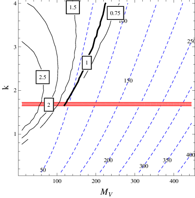
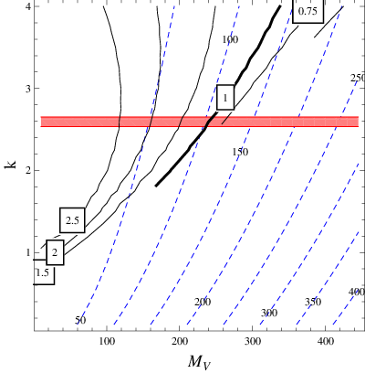
First we can see, as far as the SFOPT is concerned, the larger the VL mass $M_{V}$ is taken, the larger the Yukawa coupling $k$ needs to be. Because Boltzmann suppression effect of a few hundred GeV $M_{V}$ may decouple the new particle in the symmetric phase, significant entropy release effects for a SFOPT can only be guaranteed by a large Yuwaka mass and a large $m(\phi)/T$ shift.

Comparing to the entropy release effect in [19], we can see that for a SFOPT our required degree of freedom is much larger⁶⁶ 6 We note a convention difference and our $k=4$ corresponds to $h=2$ in [19].. This is quantitatively the most significant point of our analysis. To see clearly, with Eq. (16-20) we can write the new fermion mass squares as $M_{f_{1,2}}^{2}=M_{V}^{2}+\frac{1}{4}k^{2}\phi_{u}^{2}\mp\frac{1}{4}\sqrt{k^{4}\phi^{4}_{u}+8M^{2}_{V}k^{2}\phi^{2}_{u}}$ , or equivalently

M_{f_{1,2}}=\sqrt{M_{V}^{2}+\frac{1}{8}k^{2}\phi_{u}^{2}}\mp\frac{1}{2\sqrt{2}}k\phi_{u}.

(52)

The new sfermion mass have a similar behavior. We can understand in the following interesting picture. After EWSB the fermion masses jump from $M_{V}$ to $\sqrt{M_{V}^{2}+\frac{1}{4}k^{2}\phi_{u}^{2}}$ , and on this basis become split. The mass splitting terms $\frac{1}{2\sqrt{2}}k\phi_{u}$ make half of the VL fermions lighter than those in the symmetric phase, overcoming the common shift $M_{V}\to\sqrt{M_{V}^{2}+\frac{1}{4}k^{2}\phi_{u}^{2}}$ , while the other half heavier. In Fig. 2 we show the fully calculated finite temperature potential contribution $J_{B/F}$ instead of only the hight temperature expansions. We can refer to the $J_{B},J_{F}$ curves to see the potential change.

A shift of $M_{V}/T\to\sqrt{M_{V}^{2}+\frac{1}{4}k^{2}\phi_{u}^{2}}/T$ is exactly the entropy release effect in [19], with an effect of the representative point rise on the $J_{F}$ curve, or the thermal potential rise. Here the further new splitting of $\frac{1}{2\sqrt{2}}k\phi_{u}$ for the heavy particle will raise more the $m(\phi,T)/T$ and release more entropy, while unfortunately, the $-\frac{1}{2\sqrt{2}}k\phi_{u}$ for the light particle will have an opposite effect. A little bit more quantitative analysis indicates, because the slope of the $J_{B}/J_{F}$ curve is less at higher $m/T$ (for example, 4) than at lower $m/T$ (say, 1), the backward splitting $-\frac{1}{2\sqrt{2}}k\phi_{u}$ to lower masses always induce a larger thermal potential drop $\Delta J_{B}/\Delta J_{F}$ than the forward splitting $+\frac{1}{2\sqrt{2}}k\phi_{u}$ , and the net effect is a drop, unable to trigger the SFOPT [20]. This opposite effect will significantly compensate the $M_{V}/T\to\sqrt{M_{V}^{2}+\frac{1}{4}k^{2}\phi_{u}^{2}}/T$ effect, making the contribution to phase transition strength in our scenario much smaller than that with merely the same degree of freedom, the same soft mass and the same Yukawa, but without splitting. We will give a more general analysis in our next paper.

V.2 Higgs Mass and Light Exotic Particle Constraints

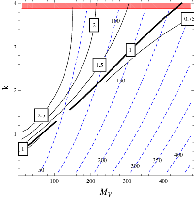
Apparently with SFOPT requirement the first two scans always give too light a new fermion, so they are ruled out. As we have already discussed, the direction we can go is to increase $M_{V}$ and $k$ . In Ref. [22] an infrared quasi fix point is pointed out, as $k\simeq 1.0$ and $h\simeq 1.2$ . Here we ignore this bound, but the bottom line is the perturbativity bound $k\lesssim 4$ . We choose to saturate the bound, then we get an almost unbroken supersymmetric VL sector⁷⁷ 7 With our MSSM parameter choices we get $\frac{M_{S}}{M_{V}}=1.019$ ., see Fig. 3

i $M_{V}$	i $M_{S}$	i $k$	i $m_{f^{\prime}_{1}}$	i $m_{f^{\prime}_{2}}$	i $m_{\tilde{f}^{\prime}_{1}}$	i $m_{\tilde{f}^{\prime}_{2}}$	i $m_{\tilde{f}^{\prime}_{3}}$	i $m_{\tilde{f}^{\prime}_{4}}$	i $\phi_{c}/T_{c}$	i $m_{h_{0}}$
70	105	1.6	17	293	80	80	304	304	2.1	126.5
100	150	1.6	32	309	116	116	329	329	1.46	126.9
230	253	2.4	102	517	116	116	528	528	0.93	125.7
475	484	4.0	241	934	259	259	939	939	0.94	126.0

Table 1: Input parameters which can realize both the SFOPT and 124-127 GeV Higgs, and the corresponding new particle masses.

The best lightest fermion mass we get is about $241$ GeV, which is still generally ruled out by heavy $t^{\prime}$ and $b^{\prime}$ quark searches, even by optimistic bounds, as mentioned in Sec. II. We will not discuss the possibility of aligned Yukawa matrix in generation basis, which make the decay mode nonstandard. On the other hand, the possibility is to relax the degeneracy between the quarks and the leptons, to make the quark sector $M_{V}$ and $M_{S}$ larger to accommodate heavier new quarks. However at first it is naively against our model assumption of $5+\overline{5}+10+\overline{10}$ of $SU(5)$ GUT, which predicts $M_{Q}=M_{U}=M_{E}$ and $M_{D}=M_{L}$ at the GUT scale. Further we numerically find that due to large zero temperature corrections, for separate quark and lepton (or generally two sets) corrections the potential usually don’t even run away from symmetric phase even at zero temperature. So we will not go into detail of that possibility.

V.3 Gluon Fusion and Higgs Diphoton Decay Constraints

We use the low energy theorem [33] for an estimation. The contributions to the loop amplitude are all proportional to $\frac{\partial}{\partial\ln v}\det\mathcal{M}$ where $\mathcal{M}$ is any of the mass matrix in Eq. (4,5). As can be see clearly in the fermion mass matrix, setting all $k^{\prime}$ s to be zeros eventually makes all the determinants independent of the Higgs VEV. The two masses of Eq. (9) are actually from the matrix $\mathcal{M}\mathcal{M}^{\dagger}$ or $\mathcal{M}^{\dagger}\mathcal{M}$ , and $\det(\mathcal{M}\mathcal{M}^{\dagger})=m_{{t^{{}^{\prime}}_{1}}}^{2}m_{{t^{{}^{\prime}}_{2}}}^{2}=M_{V}^{4}$ is independent of $\phi_{u},\phi_{d}$ . With $X_{1}=X_{2}=0$ the scalar sector has a similar behavior, but there is a residual contribution proportional to supersymmetry breaking soft parameter $m^{2}=M_{S}^{2}-M_{V}^{2}$ , namely $\det\mathcal{M}^{2}_{\tilde{U},\tilde{D},\tilde{E}}=(M_{S}^{4}+\frac{1}{2}m^{2}k^{2}\phi_{u}^{2})^{2}$ . Since we are interested in an almost supersymmetric VL sector and $m^{2}\rightarrow 0$ , the corrections to gluon fusion and Higgs diphoton decay amplitudes also vanish in this limit. So the gluon fusion Higgs production rate and Higgs diphoton decay rate are not affected. This discussion also justifies our parameter choices $k^{\prime}=0$ , $X_{1}=0$ and $X_{2}=0$ .

V.4 Peskin-Takeuchi $T$ and $S$ parameters

We perform a numerical calculation. The fermionic contribution agrees with the formulas in [22]

	$\displaystyle\Delta T$	$\displaystyle=$	$\displaystyle\frac{N_{c}}{480\pi s_{W}^{2}M_{W}^{2}M_{V}^{2}}\left(\frac{13}{4}(k^{4}v_{u}^{4}+k^{\prime 4}v_{d}^{4})+\frac{1}{2}(k^{3}k^{\prime}v_{u}^{3}v_{d}+k^{\prime 3}kv_{d}^{3}v_{u})+\frac{9}{2}k^{2}k^{\prime 2}v_{u}^{2}v_{d}^{2}\right),$		(53)
	$\displaystyle\Delta S$	$\displaystyle=$	$\displaystyle\frac{N_{c}}{30\pi M_{V}^{2}}\left(2(k^{2}v_{u}^{2}+k^{\prime 2}v_{d}^{2})+kk^{\prime}v_{u}v_{d}\Big(\frac{3}{2}+10Y_{\Phi}\Big)\right),$		(54)

with $Y_{\Phi}=-\frac{1}{3}$ for our model, while the scalar part nearly gives the same contribution for nearly unbroken supersymmetry. In particular for the last point in Tab. (1) we get $T\simeq 32.5$ and $S\simeq 0.2$ , which apparently makes it excluded. Such a large $T$ parameter contribution is because it is proportional to $k^{4}$ , and only suppressed by $M_{V}^{2}$ . On the other hand, the form of the superpotential Eq. (2) determines the custodial symmetry is violated in the maximal way, namely a light left hand up quark component always find a heavy left hand down quark component.

VI Summary

We have discussed EWBG in the MSSM extension with vector-like superfields belonging to the representation $5+\overline{5}+10+\overline{10}$ of $SU(5)$ in detail. We find the SFOPT has been ruled out by a combination of 125 GeV Higgs requirement, the direct search for the exotic fermions, the gluon fusion rate and the Higgs diphoton decay rate as well as the EW precision measurement. However, the general contribution from a (nearly) supersymmetric sector to SFOPT with minimal effect to Higgs phenomenology is still interesting.

Acknowledgements.

We would like to thank Chun Liu and Yu-Feng Zhou for a very helpful discussion. The work of X.C. was supported in part by the National Natural Science Foundation of China under nos.11375248 and 10821504, and by the National Basic Research Program of China under Grant No. 2010CB833000. The work of R.H. was supported by World Premier International Research Center Initiative (WPI Initiative), MEXT, Japan.

Appendix A one-loop corrections to the quartic coupling coefficients

Under the parameter assumptions mentioned above, the one-loop corrections to quadratic and quartic coupling coefficients in the zero temperature potential are given by

$\displaystyle\Delta m^{2}_{11}$	$\displaystyle=$	$\displaystyle\sum_{i}\frac{n_{i}}{64\pi^{2}}\alpha^{d}_{i}$	(55)
$\displaystyle\Delta m^{2}_{22}$	$\displaystyle=$	$\displaystyle\sum_{i}\frac{n_{i}}{64\pi^{2}}\alpha^{u}_{i}$	(56)
$\displaystyle\Delta\lambda_{1}$	$\displaystyle=$	$\displaystyle\sum_{i}\frac{n_{i}}{64\pi^{2}}\beta^{d}_{i}+\frac{1}{16\pi^{2}}\Bigl\{-3y_{t}^{4}\frac{\mu^{4}}{12M_{s}^{4}}$	(57)
		$\displaystyle+\sum_{i}N_{C_{i}}\Bigl[k^{{}^{\prime}4}_{i}\Bigl(\mathrm{ln}\frac{M^{2}_{S}}{M^{2}_{V}}-\frac{1}{6}(5-\frac{M^{2}_{V}}{M^{2}_{S}})(1-\frac{M^{2}_{V}}{M^{2}_{S}})+\hat{X}^{2}_{1}(1-\frac{M^{2}_{V}}{3M^{2}_{S}})-\frac{\hat{X}^{4}_{1}}{12}\Bigr)\Bigr]\Bigr\}$	(57)
$\displaystyle\Delta\lambda_{2}$	$\displaystyle=$	$\displaystyle\sum_{i}\frac{n_{i}}{64\pi^{2}}\beta^{u}_{i}+\frac{1}{16\pi^{2}}\Bigl\{3y_{t}^{4}\Bigl[\ln(\frac{\tilde{m}^{2}_{t}}{m^{2}_{t}})+\frac{A_{t}^{2}}{\tilde{m}^{2}_{t}}(1-\frac{A_{t}^{2}}{12\tilde{m}^{2}_{t}})-\frac{\mu^{4}}{12\tilde{m}^{4}_{t}}\Bigr]$	(58)
		$\displaystyle+\sum_{i}N_{C_{i}}\Bigl[k^{4}_{i}\Bigl(\mathrm{ln}\frac{M^{2}_{S}}{M^{2}_{V}}-\frac{1}{6}(5-\frac{M^{2}_{V}}{M^{2}_{S}})(1-\frac{M^{2}_{V}}{M^{2}_{S}})+\hat{X}^{2}_{1}(1-\frac{M^{2}_{V}}{3M^{2}_{S}})-\frac{\hat{X}^{4}_{1}}{12}\Bigr)\Bigr]\Bigr\}$	(58)
$\displaystyle\Delta\lambda_{3}$	$\displaystyle=$	$\displaystyle\sum_{i}\frac{n_{i}}{64\pi^{2}}\beta^{ud}_{i}+\frac{1}{16\pi^{2}}\Bigl\{3\Bigl[\frac{y_{t}^{4}}{2}\frac{\mu^{2}}{\tilde{m}^{2}_{t}}(1-\frac{A_{t}^{2}}{2\tilde{m}^{2}_{t}})\Bigr]$	(59)
		$\displaystyle+\sum_{i}N_{C_{i}}\Bigl[k^{2}_{i}k^{{}^{\prime}2}_{i}\Bigl(-(1-\frac{M^{2}_{V}}{M^{2}_{S}})^{2}-\frac{1}{3}(\hat{X}_{1}+\hat{X}_{2})^{2}\Bigr)\Bigr]\Bigr\}$	(59)
$\displaystyle\Delta\lambda_{6}$	$\displaystyle=$	$\displaystyle\frac{1}{16\pi^{2}}\Bigl\{3y_{t}^{4}\frac{\mu^{3}A_{t}}{12\tilde{m}^{4}_{t}}$	(60)
		$\displaystyle+\sum_{i}N_{C_{i}}\Bigl[k^{{}^{\prime}3}_{i}k_{i}\Bigl(-\frac{2}{3}(2-\frac{M^{2}_{V}}{M^{2}_{S}})(1-\frac{M^{2}_{V}}{M^{2}_{S}})-\frac{1}{3}(2\hat{X}^{2}_{2}+\hat{X}_{1}\hat{X}_{2})\Bigr)\Bigr]\Bigr\}$	(60)
$\displaystyle\Delta\lambda_{7}$	$\displaystyle=$	$\displaystyle\frac{1}{16\pi^{2}}\Bigl\{3y_{t}^{4}\frac{\mu A_{t}}{\tilde{m}^{2}_{t}}(-\frac{1}{2}+\frac{A_{t}^{2}}{12\tilde{m}^{2}_{t}})$	(61)
		$\displaystyle+\sum_{i}N_{C_{i}}\Bigl[k^{3}_{i}k^{{}^{\prime}}_{i}\Bigl(-\frac{2}{3}(2-\frac{M^{2}_{V}}{M^{2}_{S}})(1-\frac{M^{2}_{V}}{M^{2}_{S}})-\frac{1}{3}(2\hat{X}^{2}_{1}+\hat{X}_{1}\hat{X}_{2})\Bigr)\Bigr]\Bigr\}$	(61)

References

[1] M. E. Shaposhnikov, Nucl. Phys. B 287, 757 (1987).
[2] M. Fukugita and T. Yanagida, Phys. Lett. B 174, 45 (1986).
[3] W. Buchmuller, P. Di Bari and M. Plumacher, Nucl. Phys. B 665, 445 (2003) [hep-ph/0302092].
[4] M. Yoshimura, Phys. Rev. Lett. 41, 281 (1978) [Erratum-ibid. 42, 746 (1979)].
[5] S. Dimopoulos and L. Susskind, Phys. Rev. D 18, 4500 (1978).
[6] S. Weinberg, Phys. Rev. Lett. 42, 850 (1979).
[7] W. Buchmuller and M. Plumacher, Int. J. Mod. Phys. A 15, 5047 (2000) [hep-ph/0007176].
[8] A. G. Cohen, D. B. Kaplan and A. E. Nelson, Ann. Rev. Nucl. Part. Sci. 43, 27 (1993) [hep-ph/9302210]; M. Quiros, Helv. Phys. Acta 67, 451 (1994); V. A. Rubakov and M. E. Shaposhnikov, Usp. Fiz. Nauk 166, 493 (1996) [Phys. Usp. 39, 461 (1996)] [hep-ph/9603208]; M. S. Carena and C. E. M. Wagner, hep-ph/9704347; A. Riotto and M. Trodden, Ann. Rev. Nucl. Part. Sci. 49, 35 (1999)[hep-ph/9901362]; M. Quiros and M. Seco, Nucl. Phys. Proc. Suppl. 81, 63 (2000) [hep-ph/9903274].
[9] V. A. Kuzmin, V. A. Rubakov and M. E. Shaposhnikov, Phys. Lett. B 155, 36 (1985).
[10] M. E. Carrington, Phys. Rev. D 45, 2933 (1992); P. B. Arnold and O. Espinosa, [Erratum-ibid. D 50, 6662 (1994)] [hep-ph/9212235].
[11] S. Y. .Khlebnikov and M. E. Shaposhnikov, Nucl. Phys. B 308, 885 (1988); F. R. Klinkhamer and N. S. Manton, Phys. Rev. D 30, 2212 (1984); M. Dine, P. Huet and R. L. Singleton, Jr, Nucl. Phys. B 375, 625 (1992); M. Dine, R. G. Leigh, P. Huet, A. D. Linde and D. A. Linde, Phys. Lett. B 283, 319 (1992) [hep-ph/9203201]; P. B. Arnold, Phys. Rev. D 46, 2628 (1992) [hep-ph/9204228]; J. E. Bagnasco and M. Dine, Phys. Lett. B 303, 308 (1993) [hep-ph/9212288]; K. Kajantie, K. Rummukainen and M. E. Shaposhnikov, Nucl. Phys. B 407, 356 (1993) [hep-ph/9305345]; K. Kajantie, M. Laine, K. Rummukainen and M. E. Shaposhnikov, Nucl. Phys. B 466, 189 (1996) [hep-lat/9510020].; G. R. Farrar and M. E. Shaposhnikov, Phys. Rev. Lett. 70, 2833 (1993) [Erratum-ibid. 71, 210 (1993)] [hep-ph/9305274].
[12] M. B. Gavela, P. Hernandez, J. Orloff and O. Pene, Mod. Phys. Lett. A 09, 795 (1994) [hep-ph/9312215, hep-ph/9312215]; M. B. Gavela, P. Hernandez, J. Orloff, O. Pene and C. Quimbay, Nucl. Phys. B 430, 382 (1994) [hep-ph/9406289]; P. Huet and E. Sather, Phys. Rev. D 51, 379 (1995) [hep-ph/9404302].
[13] G. Aad et al. [ATLAS Collaboration], Phys. Lett. B 716, 1 (2012) [arXiv:1207.7214 [hep-ex]].
[14] S. Chatrchyan et al. [CMS Collaboration], Phys. Lett. B 716, 30 (2012) [arXiv:1207.7235 [hep-ex]].
[15] M. S. Carena, M. Quiros and C. E. M. Wagner, Phys. Lett. B 380, 81 (1996) [hep-ph/9603420].
[16] D. Delepine, J. M. Gerard, R. Gonzalez Felipe and J. Weyers, Phys. Lett. B 386, 183 (1996) [hep-ph/9604440].
[17] D. Curtin, P. Jaiswal and P. Meade, JHEP 1208, 005 (2012) [arXiv:1203.2932 [hep-ph]]; T. Cohen, D. E. Morrissey and A. Pierce, Phys. Rev. D 86, 013009 (2012) [arXiv:1203.2924 [hep-ph]]; M. Carena, G. Nardini, M. Quiros and C. E. M. Wagner, JHEP 1302, 001 (2013) [arXiv:1207.6330 [hep-ph]].
[18] D. J. H. Chung, A. J. Long and L. -T. Wang, Phys. Rev. D 87, 023509 (2013) [arXiv:1209.1819 [hep-ph]].
[19] M. S. Carena, A. Megevand, M. Quiros and C. E. M. Wagner, Nucl. Phys. B 716, 319 (2005) [hep-ph/0410352].
[20] R. Huo, arXiv:1305.1973 [hep-ph].
[21] R. Fok and G. D. Kribs, Phys. Rev. D 78, 075023 (2008) [arXiv:0803.4207 [hep-ph]].
[22] S. P. Martin, Phys. Rev. D 81, 035004 (2010) [arXiv:0910.2732 [hep-ph]]; S. P. Martin and J. D. Wells, Phys. Rev. D 86, 035017 (2012) [arXiv:1206.2956 [hep-ph]].
[23] C. Liu, Phys. Rev. D 80, 035004 (2009) [arXiv:0907.3011 [hep-ph]]; X. Chang, C. Liu and Y. -L. Tang, Phys. Rev. D 87, no. 7, 075012 (2013) [arXiv:1303.7055 [hep-ph]]; A. Joglekar, P. Schwaller and C. E. M. Wagner, JHEP 1307, 046 (2013) [arXiv:1303.2969 [hep-ph]].
[24] J. Beringeret al. (Particle Data Group), Phys. Rev. D86, 010001 (2012).
[25] M. E. Peskin and T. Takeuchi, Phys. Rev. D 46, 381 (1992); G. Cynolter and E. Lendvai, Eur. Phys. J. C 58, 463 (2008) [arXiv:0804.4080 [hep-ph]].
[26] P. H. Frampton, P. Q. Hung and M. Sher, Phys. Rept. 330, 263 (2000) [hep-ph/9903387]; S. Nandi and A. Soni, Phys. Rev. D 83, 114510 (2011) [arXiv:1011.6091 [hep-ph]]; G. D. Kribs, T. Plehn, M. Spannowsky and T. M. P. Tait, Phys. Rev. D 76, 075016 (2007) [arXiv:0706.3718 [hep-ph]].
[27] K. S. Babu, I. Gogoladze, M. U. Rehman and Q. Shafi, Phys. Rev. D 78, 055017 (2008) [arXiv:0807.3055 [hep-ph]].
[28] H. E. Haber and R. Hempfling, Phys. Rev. D 48, 4280 (1993) [hep-ph/9307201].
[29] K. Rao and D. Whiteson, Phys. Rev. D 86, 015008 (2012) [arXiv:1204.4504 [hep-ph]].
[30] D. Buskulic et al. [ALEPH Collaboration], Phys. Lett. B 384 (1996) 439.
[31] D. Comelli and J. R. Espinosa, Phys. Rev. D 55 (1997) 6253 [hep-ph/9606438].
[32] C. L. Wainwright, Comput. Phys. Commun. 183, 2006 (2012) [arXiv:1109.4189 [hep-ph]].
[33] J. F. Gunion, H. E. Haber, G. L. Kane and S. Dawson, Front. Phys. 80, 1 (2000); M. A. Shifman, A. I. Vainshtein, M. B. Voloshin and V. I. Zakharov, Sov. J. Nucl. Phys. 30, 711 (1979) [Yad. Fiz. 30, 1368 (1979)].
[34] C. Bal¨¢zs, A. Mazumdar, E. Pukartas and G. White, JHEP 1401, 073 (2014) [arXiv:1309.5091 [hep-ph]].