Algorithmic Aspects of Regular Graph Covers
with Applications to Planar GraphsThanks:
The conference version of this paper appeared in ICALP 2014.
The first three authors are supported by the ESF Eurogiga project GraDR as GAČR GIG/11/E023,
the fourth author by the ESF Eurogiga project GReGAS as the APVV project ESF-EC-0009-10 and by VEGA 1/0621/11.
The first author is also supported by the project Kontakt LH12095 and the second author by GAČR 14-14179S.
The second and the third authors are also supported by Charles University as GAUK 196213.
Abstract
A graph covers a graph if there exists a locally bijective homomorphism from to . We deal with regular covers in which this locally bijective homomorphism is prescribed by an action of a subgroup of . Regular covers have many applications in constructions and studies of big objects all over mathematics and computer science.
We study computational aspects of regular covers that have not been addressed before. The decision problem RegularCover asks for two given graphs and whether regularly covers . When , this problem becomes Cayley graph recognition for which the complexity is still unresolved. Another special case arises for when it becomes the graph isomorphism problem. Therefore, we restrict ourselves to graph classes with polynomially solvable graph isomorphism.
Inspired by Negami, we apply the structural results used by Babai in the 1970’s to study automorphism groups of graphs. Our main result is the following FPT meta-algorithm: Let be a class of graphs such that the structure of automorphism groups of 3-connected graphs in is simple. Then we can solve RegularCover for -inputs in time where denotes the number of the edges of . As one example of , this meta-algorithm applies to planar graphs. In comparison, testing general graph covers is known to be NP-complete for planar inputs even for small fixed graphs such as or . Most of our results also apply to general graphs, in particular the complete structural understanding of regular covers for 2-cuts.
1 Introduction
The notion of covering originates in topology as a notion of local similarity of two topological surfaces. For instance, consider the unit circle and the real line. Globally, these two surfaces are not the same, they have different properties, different fundamental groups, etc. But when we restrict ourselves to a small part of the circle, it looks the same as a small part of the real line; more precisely the two surfaces are locally homeomorphic, and thus they share the local properties. The notion of covering formalizes this property of two surfaces being locally the same.
More precisely, suppose that we have two topological spaces: a big one and a small one . We say that covers if there exists a mapping called a covering projection which locally preserves the structure of . For instance, the mapping from the real line to the unit circle is a covering projection. The existence of a covering projection ensures that looks locally the same as ; see Figure 1a.
In this paper, we study coverings of graphs in a more restricting version called regular covering, for which the covering projection is described by an action of a group; see Section 2 for the formal definition. If regularly covers , then we say that is a quotient of .

1.1 Applications of Graph Coverings
Suppose that covers and we have some information about one of the objects. How much knowledge does translate to the other object? It turns out that quite a lot, and this makes covering a powerful technique with many diverse applications. The big advantage of regular coverings is that they can be efficiently described and many properties easily translate between the objects. We sketch some applications now.
Powerful Constructions. The reverse of covering called lifting can be applied to small objects in order to construct large objects of desired properties. For instance, the well-known Cayley graphs are large objects which can be described easily by a few elements of a group. Let be a Cayley graph generated by elements of a group . The vertices of correspond to the elements of and the edges are described by actions of on by left multiplication; each defines a permutation on and we put edges along the cycles of this permutation. See Figure 1b for an example. Cayley graphs were originally invented to study the structure of groups [13].
In the language of coverings, every Cayley graph with an involution-free generating set can be described as a lift of a one vertex graph with loops labeled . Regular covers can be viewed as a generalization of Cayley graphs where the small graph can contain more then one vertex. For example, the famous Petersen graph can be constructed as a lift of a two vertex graph , see Figure 2a. These two vertices are necessary as it is known that Petersen graph is not a Cayley graph. Figure 2b shows a simple construction [36] of the Hoffman-Singleton graph [27] which is a 7-regular graph with 50 vertices. Notice that from this construction it is immediately apparent that the Hoffman-Singleton graph contains many induced copies of the Petersen graph. (In fact, it contains 525 copies of it.)

The Petersen and the Hoffman-Singleton graphs are extremal graphs for the degree-diameter problem: Given integers and , find a maximal graph with diameter and degree . In general, the size of is not known. Many currently best constructions are obtained using the covering techniques [37].
Further applications employ the fact that nowhere-zero flows, vertex and edge colorings, eigenvalues and other graph invariants lift along a covering projection. In history, two main applications are the solution of the Heawood map coloring problem [39, 23] and construction of arbitrary large highly symmetrical graphs [7].
Models of Local Computation. These and similar constructions have many practical applications in designing highly efficient computer networks [15, 1, 6, 10, 11, 12, 24, 43] since these networks can be efficiently described/constructed and have many strong properties. In particular, networks based on covers of simple graphs allow fast parallelization of computation as described e.g. in [9, 2, 3].
Simplifying Objects. Regular covering can be also applied in the opposite way, to project big objects onto smaller ones while preserving some properties. One way is to represent a class of objects satisfying some properties as quotients of the universal object of this property. For instance, this was used in the study of arc-transitive cubic graphs [22], and the key point is that universal objects are much easier to work with. This idea is commonly used in fields such as Riemann surfaces [17] and theoretical physics [30].
1.2 Complexity Aspects
In the constructions we described, the covers are regular and satisfy additional algebraic properties. The reason is that regular covers are easier to describe. In this paper, we initiate the study of the computational complexity of regular covering.
| Problem: | RegularCover |
|---|---|
| Input: | Connected graphs and . |
| Output: | Does regularly cover ? |
Relations to Covers. This problem is closely related to the complexity of general covering which was widely studied before. We try to understand how much the additional algebraic structure changes the computational complexity. Study of the complexity of general covers was pioneered by Bodlaender [9] in the context of networks of processors in parallel computing, and for fixed target graph was first asked by Abello et al. [19]. The problem -Cover asks for an input graph whether it covers a fixed graph . The general complexity is still unresolved but papers [31, 20] show that it is NP-complete for every -regular graph where . (For a survey of the complexity results, see [21].)
The complexity results concerning graph covers are mostly NP-complete. In our impression, the additional algebraic structure of regular graph covers makes the problem easier, as shown by the following two contrasting results. The problem -Cover remains NP-complete for several small fixed graphs (such as , ) even for planar inputs [8]. On the other hand, our main result is that the problem RegularCover is fixed-parameter tractable in the number of edges of for every planar graph and for every .
Two additional problems of finding lifts and quotients, closely related to RegularCover, are considered in Section 2.3.
Relations to Cayley Graphs and Graph Isomorphism. The notion of regular covers builds a bridge between two seemingly different problems. If the graph consists of a single vertex, it corresponds to recognizing Cayley graphs which is still open; a polynomial-time algorithm is known only for circulant graphs [16]. When both graphs and have the same size, we get graph isomorphism testing. Our results are far from this but we believe that better understanding of regular covering can also shed new light on these famous problems.
Theoretical motivation for studying graph isomorphism is very similar to RegularCover. For practical instances, one can solve the isomorphism problem very efficiently using various heuristics. But polynomial-time algorithm working for all graph is not known and it is very desirable to understand the complexity of graph isomorphism. It is known that testing graph isomorphism is equivalent to testing isomorphism of general mathematical structures [25]. The notion of isomorphism is widely used in mathematics when one wants to show that two seemingly different mathematical structures are the same. One proceeds by guessing a mapping and proving that this mapping is an isomorphism. The natural complexity question is whether there is a better way in which one algorithmically derives an isomorphism. Similarly, regular covering is a well-known mathematical notion which is algorithmically interesting and not understood.
Further, a regular covering is described by a semiregular subgroup of the automorphism group . Therefore it seems to be closely related to computation of since one should have a good understanding of this group first to solve the regular covering problem. The problem of computing automorphism groups is known to be closely related to graph isomorphism.
Homomorphisms and CSP. Since regular covering is a restricted locally bijective homomorphism, we give an overview of complexity results concerning homomorphisms and general coverings. Hell and Nešetřil [26] studied the problem -Hom which asks whether there exists a homomorphism between an input graph and a fixed graph . Their celebrated dichotomy result for simple graphs states that the problem -Hom is polynomially solvable if is bipartite and it is NP-complete otherwise. Homomorphisms can be described in the language of constraint satisfaction (CSP), and the famous dichotomy conjecture [18] claims that every CSP is either polynomially solvable, or NP-complete.
1.3 Our Results
Let be a class of connected multigraphs. By we denote the class of all regular quotients of graphs of (note that ). For instance for equal to planar graphs, the class is – according to the Negami’s Theorem [38] – the class of projective planar graphs. We consider four properties of , for formal definitions see Section 2:
- (P0)
The class is closed under taking subgraphs and under replacing connected components attached to 2-cuts by edges.
- (P1)
The graph isomorphism problem is solvable in polynomial time for and .
- (P2)
For a 3-connected graph , the group and all its semiregular subgroups can be computed in polynomial time. Here by semiregularity, we mean that the action of has no non-trivial stabilizers of the vertices.
- (P3)
Let and be 3-connected graphs of , possibly with colored and directed edges. Let the vertices of be further colored by , and let be equipped with a list of possible colors for each vertex (the coloring is not necessarily proper). We can test in polynomial time whether there exists a color-compatible isomorphism , i.e. an isomorphism such that the colors and orientations of edges are preserved and for every , we have . (The existence of such an isomorphism is denoted by .)
As we prove in Section 6, these four properties are tailored for the class of planar graphs. (But the proof of the property (P3) is non-trivial, based on the result of [32].) Negami’s Theorem [38] dealing with regular covers of planar graphs is one of the oldest results in topological graph theory; therefore we decided to start the study of computational complexity of RegularCover for planar graphs. Our algorithm, however, applies to a wider class of graphs.
We use the complexity notation which omits polynomial factors. Our main result is the following FPT meta-algorithm:
Theorem 1.1
Let be a class of graphs satisfying (P0) to (P3). Then there is an FPT algorithm for RegularCover for -inputs in the parameter , running in time where is the number of edges of .
It is important that most of our results apply to general graphs. We wanted to generalize the result of Babai [4] which states that it is sufficient to solve graph isomorphism for 3-connected graphs. Our main goal was to understand how regular covering behaves with respect to vertex 1-cuts and 2-cuts. Concerning 1-cuts, regular covering behaves non-trivially only on the central block of , so they are easy to deal with. But we show that regular covering can behave highly complex on 2-cuts. From structural point of view, we give a complete description of this behaviour. Algorithmically, we solve computation only partially and we need several other assumptions to get an efficient algorithm.
Planar graphs are very important and also well studied in connection to coverings. Negami’s Theorem [38] dealing with regular covers of planar graphs is one of the oldest results in topological graph theory; therefore we decided to start the study of computational complexity of RegularCover for planar graphs. In particular, our theory applies to planar graphs since they satisfy (P0) to (P3).
Corollary 1
For a planar graph , RegularCover can be solved in time .
Our Approach. We quickly sketch our approach. The meta-algorithm proceeds by a series of reductions replacing parts of the graphs by edges. These reductions are inspired by the approach of Negami [38] and turn out to follow the same lines as the reductions introduced by Babai for studying automorphism groups of planar graphs [4, 5]. Since the key properties of the automorphism groups are preserved by the reductions, computing automorphism groups can be reduced to computing them for 3-connected graphs [4]. In [29, 28], this is used to compute automorphism groups of planar graphs since the automorphism groups of 3-connected planar graphs are the automorphism groups of tilings of the sphere, and are well-understood.
The RegularCover problem is more complicated, and we use the following novel approach. When the reductions reach a 3-connected graph, the natural next step is to compute all its quotients; there are polynomially many of them according to (P2). What remains is the most difficult part: To test for each quotient whether it corresponds to after unrolling the reductions. This process is called expanding and the issue here is that there may be exponentially many different ways to expand the graph, so we have to test in a clever way whether it is possible to reach . Our algorithm consists of several subroutines, most of which we indeed can perform in polynomial time. Only one subroutine (finding a certain “generalized matching”) we have not been able to solve in polynomial time.
This slow subroutine can be avoided in some cases:
Corollary 2
If the -graph is 3-connected or if is odd, then the meta-algorithm of Theorem 1.1 can be modified to run in polynomial time.
Structure. This paper is organized as follows. In Section 2, we introduce the formal notation used in this paper. In Section 3, we introduce atoms which are the key objects of this paper. In Section 4, we describe structural properties of reductions via atoms, and expansions of constructed quotient graphs. In Section 5, we use these structural properties to create the meta-algorithm of Theorem 1.1. Finally, in Section 6 we deal with specific properties of planar graphs and show that the class of planar graphs satisfies (P0) to (P3). In Conclusions, we describe open problems and possible extensions of our results. See Section 2.4 for more detailed overview of the main steps.
2 Definitions and Preliminaries
A multigraph is a pair where is a set of vertices and is a multiset of edges. We denote by and by . The graph can possibly contain parallel edges and loops, and each loop at is incident twice with the vertex . (So it contributes by two to the degree of .) Each edge gives rise to two half-edges, one attached to and the other to . We denote by the collection of all half-edges. We denote by and clearly . As quotients, we sometime obtain graphs containing half-edges with free ends (missing the opposite half-edges).
We consider graphs with colored edges and also with three different edge types (directed edges, undirected edges and a special type called halvable edges). It might seem strange to consider such general objects. But when we apply reductions, we replace parts of the graph by edges and the colors encode isomorphism classes of replaced parts. This allows the algorithm to work with smaller reduced graphs and deduce some structure of the original large graph. So even if the input graphs and are simple, the more complicated multigraphs are naturally constructed.
2.1 Automorphisms and Groups
Automorphisms. We state the definitions in a very general setting of multigraphs and half-edges. An automorphism is fully described by a permutation preserving edges and incidences between half-edges and vertices. Thus, induces two permutations and connected together by the very natural property for every . In most of situations, we omit subscripts and simply use or . In addition, when we work with colored graphs, we require that an automorphism preserves the colors.
Groups. We assume that the reader is familiar with basic properties of groups; otherwise see [40]. We denote groups by Greek letters as for instance . We use the following notation for standard groups:
- •
for the symmetric group of all -element permutations,
- •
for the cyclic group of integers modulo ,
- •
for the dihedral group of the symmetries of a regular -gon, and
- •
for the group of all even -element permutations.
Automorphism Groups. Groups are quite often studied in the context of group actions, since their origin is in studying symmetries of mathematical objects. A group acts on a set in the following way. Each permutes the elements of , and the action is described by a mapping usually satisfying further properties that arise naturally from the structure of .
In the language of graphs, an example of such an action is the group of all automorphisms of , denoted by . Each element acts on , permutes its vertices, edges and half-edges while it preserves edges and incidences between the half-edges and the vertices.
The orbit of a vertex is the set of all vertices , and the orbit of an edge is defined similarly as . The stabilizer of is the subgroup of all automorphisms which fix . An action is called semiregular if it has no non-trivial (i.e., non-identity) stabilizers of both vertices and half-edges. Note that the stabilizer of an edge in a semiregular action may be non-trivial, since it may contain an involution transposing the two half-edges. We say that a group is semiregular if the associated action is semiregular.
2.2 Coverings

A graph covers a graph (or is a cover of ) if there exists a locally bijective homomorphism called a covering projection. A homomorphism from to is given by a mapping preserving edges and incidences between half-edges and vertices. It induces two mappings and such that for every . The property to be local bijective states that for every vertex the mapping restricted to the half-edges incident with is a bijection. Figure 3 contains two examples of graph covers. Again, we mostly omit subscripts and just write or . A fiber of a vertex is the set , i.e., the set of all vertices that are mapped to , and similarly for fibers over edges and half-edges.
The Unique Walk Lifting Property. Let be an edge which is not a loop. Then the set corresponds to a perfect matching between the fibers and . And if is a loop, then the set is a union of disjoint cycles which cover exactly . Figure 4 shows examples. In general for a subgraph of , the correspondence between and its preimages in is called lifting.

Let be a walk in . Then consists of copies of . Suppose that we fix as the start one vertex in the fiber . Due to the local bijectiveness of , there is exactly one edge incident with it which maps to , so is now uniquely determined, and so on for and the other vertices of . When we proceed in this way, the rest of the walk is determined. This important property of every covering is called the unique walk lifting property.
We adopt the standard assumption that both and are connected. Then as a simple corollary we get that all fibers of are of the same size. To see that, observe that a path in is lifted to disjoint paths in . For , consider a path between them. Then the paths in define a bijection between the fibers and . In other words, for some which is the size of each fiber, and we say that is a -fold cover of .
Covering Transformation Groups. Every covering projection defines a special subgroup of called covering transformation group . It consists of all automorphisms which preserve the fibers of , i.e., for every , the vertices and belong to one fiber. Consider the graphs from Figure 3. For the graph , we have and . And has but is trivial; and we note that it is often the case that a covering projection has only one fiber-preserving automorphism, the trivial one.
Now suppose that . Observe that a single choice of the image of one vertex fully determines . This follows from the unique walk lifting property. Let and consider some path connecting and in . This path corresponds to a path in . Now we lift and according to the unique walk lifting property, there exists a unique path which starts in . But since is an automorphism and it maps to , then has to be equal . In other words, we just proved that is semiregular.
Regular Coverings. We want to consider coverings which are highly symmetrical. For examples from Figure 3, the covering is more symmetric than . The size of is a good measure of symmetricity of the covering . Since is semiregular, it easily follows that for any -fold covering . A covering is regular if . In Figure 3, the covering is regular since , and the covering is not regular since .
We use the following definition of regular covering. Let be any semiregular subgroup of . It defines a graph called a regular quotient (or simply quotient) of as follows: The vertices of are the orbits of the action on , the half-edges of are the orbits of the action on . A vertex-orbit is incident with a half-edge-orbit if and only if the vertices of are incident with the half-edges of . (Because the action of is semiregular, each vertex of is incident with exactly one half-edge of , so this is well defined.) We naturally construct by mapping the vertices to its vertex-orbits and half-edges to its half-edge-orbits. Concerning an edge , it is mapped to an edge of if the two half-edges belong to different half-edge-orbits of . If they belong to the same half-edge-orbits, it corresponds to a standalone half-edge of .
Since acts semiregularly on , one can prove that is a -fold regular covering with . For the graphs and of Figure 3, we get for which “rotates the cycle by three vertices”. As a further example, Figure 5 geometrically depicts all quotients of the cube graph.

2.3 Fundamental Complexity Properties of Coverings
We establish fundamental complexity properties of regular covering and also general covering. Our goal is to highlight similarities with the graph isomorphism problem. Also we discuss other variants of the RegularCover problem.
Belonging to NP. The general -Cover problem is clearly in NP since one can just test in polynomial time whether a given mapping is a locally bijective homomorphism. Not so obviously, the same holds for the RegularCover problem.
Lemma 1
The problem RegularCover is in NP.
Proof
One just needs to use a suitable definition of regular covering. As stated above, regularly covers , if and only if there exists a semiregular subgroup of such that . As the certificate, we just give permutations, one for each element of , and the isomorphism between and . We can easily check whether these permutations define a group , and whether acts semiregularly on . Further, the given isomorphism allows to check whether the constructed is isomorphic to . Clearly, this certificate is polynomially large and can be verified in polynomial time.∎
One can prove even a stronger result:
Lemma 2
For a mapping , we can test whether it is a regular covering in polynomial time.
Proof
Testing whether is a covering can clearly be done in polynomial time. It remains to test regularity. Choose an arbitrary spanning tree of . Since is a covering, then is a disjoint union of isomorphic copies of . We number the vertices of the fibers according to the spanning trees, i.e., such that . This induces a numbering of the half-edges of each fiber over a half-edge of , following the incidences between half-edges and vertices. For every half-edge , we define a permutation of taking to if there is a half-edge in such that the edge corresponds to .
It remains to test whether the size of the group generated by all , where , is of size exactly . From the theory of permutation groups, since is assumed to be connected, it follows that the action of is transitive. Therefore its size is at least , and the action is regular if and only if it is exactly .∎
The constructed permutations associated with are known in the literature [23] as permutation voltage assigments associated with .
Other Variants. In the RegularCover problem, the input gives two graphs and and we ask for an existence of a regular covering from to . There are two other reasonable variants of this problem we discuss now. The input can specify only one of the two graphs and ask for existence of the other graph of, say, a given size.
First, suppose that only is given and we ask whether a -fold cover of exists. This is called lifting and the answer is always positive. The theory of covering describes a technique called voltage assignment which can be applied to generate all -folds . We do not deal with lifting in this paper, but there are nevertheless many interesting computational questions with important applications. For instance, one can try to generate efficiently all lifts up to isomorphism; this is not trivial since different voltage assignments might lead to isomorphic graphs. Also, one may ask for existence of a lift with some additional properties.
The other variant gives only and asks for existence of a quotient which is regularly covered by and . This problem is NP-complete even for fixed , proved in a different language by Lubiw [33]. Lubiw shows that testing existence of a fixed-point free involutory automorphism is NP-complete which is equivalent to existence of a half-quotient . We sketch hers reduction from -Sat. Each variable is represented by an even cycle attached to the rest of the graph. Each cycle has two possible regular quotients, either a cycle of half length (obtained by the rotation), or a path of half length with attached half-edges (obtained by a reflection through opposite edges). Each of these quotients represents one truth assignment of the corresponding variable. To distinguish variables, distinct gadgets are attached to the cycles. These variable gadgets are attached to clause gadgets. Naturally, one can construct a quotient of the clause gadget if and only if at least one literal is satisfied.
One should ask whether this reduction also implies NP-completeness for the RegularCover problem. Since the input gives also a graph , one can decode the assignment of the variables from it, and thus this reduction does not work. We conjecture that no similar reduction with a fixed can be constructed for RegularCover since we believe that for a fixed the problem of counting the number of regular coverings between and can be solved using polynomially-many instances of RegularCover. In complexity theory, it is believed that the counting version of no NP-complete problem satisfies this. Similar evidence was used by Mathon [35] to show that graph isomorphism is unlikely NP-complete, and as a work in progress we believe that a similar argument can be applied to RegularCover.
The results of this paper also show that the reduction of Lubiw cannot be modified for planar inputs . Our algorithmic and structural insights allow an efficient enumeration of all quotients of a given planar graph . On the other hand, the hardness result of Lubiw states that to solve the RegularCover problem in general, one has to work with both graphs and from beginning. Our algorithm starts only with and tries to match its quotients to only in the end. Nevertheless, some modifications in this directions, not necessary for planar graphs, would be possible.
2.4 Overview of the Main Steps
We now give a quick overview of the paper.
The main idea is the following. If the input graph is 3-connected, using our assumptions the RegularCover problem is trivially solvable. Otherwise, we proceed by a series of reductions, replacing parts of the graph by edges, essentially forgetting details of the graph. We end-up with a primitive graph which is either 3-connected, or very simple (a cycle or ). The reductions are done in such a way that no essential information of semiregular actions is lost.
Inspired by Negami [38] and Babai [5], we introduce in Section 3 the most important definition of an atom. Atoms are inclusion-minimal subgraphs which cannot be further simplified and are essentially 3-connected. Our strategy for reductions is to detect the atoms and replace them by edges. In this process, we remove details from the graph but preserve its overall structure. Our definition of atoms is quite technical, dealing with many details necessary for the next sections.
When the graph is not 3-connected, we consider its block-tree. The central block plays the key role in every regular covering projection. The reason is that the covering behaves non-trivially only on this central block; the remaining blocks are isomorphically preserved in . Therefore the atoms are defined with respect to the central block. We distinguish three types of atoms:
- •
Proper atoms are inclusion-minimal subgraphs separated by a 2-cut inside a block.
- •
Dipoles are formed by the sets of all parallel edges joining two vertices.
- •
Block atoms are blocks which are leaves of the block-tree, or stars of all pendant edges attached to a vertex. The central block is never a block atom.
In Section 4, we deal with two transformations of graphs called reduction and expansion. The graph is reduced by replacing its atoms by edges; for proper atoms and dipoles inside the blocks, for block atoms by pendant edges. Further these edges are colored according to isomorphism classes of the atoms. This way the reduction omits unimportant details from the graph but its key structure is preserved. We apply a series of reductions till we obtain a graph called primitive which contains no atoms. We show that the reduction preserves essentially the automorphism group. More precisely, is a factor-group of ; the action of inside the atoms is lost by the factorization.
The other transformation called expansion is applied to the quotient graphs. The goal of expansion is to revert the reduction, so it replaces colored edges back by atoms. To do this, we have to understand how regular covering behaves with respect to atoms. Inspired by Negami [38], we show that each proper atom/dipole has three possible types of quotients that we call an edge-quotient, a loop-quotient and a half-quotient. The edge-quotient and the loop-quotient are uniquely determined but an atom may have many non-isomorphic half-quotients.
When the primitive graph is reached, all semiregular subgroups of are computed and for each one a quotient is constructed. Our goal is to understand all graphs to which can be expanded, as depicted in the following diagram:
The constructed quotients contain colored edges, loops and half-edges corresponding to atoms. Each half-edge in is created from a halvable edge if an automorphism of fixes this halvable edge and exchanges its endpoints. Roughly speaking it corresponds to cutting the edge in half. We show that every possible expansion of a quotient from can be constructed by replacing the colored edges by the edge-quotients of the atoms, the colored loops by the loop-quotients and the color half-edges by some choices of half-quotients. This gives the complete structural description of all graphs which can be reached from by expansion. Half-edges of can arise only in expansions of half-edges of .
In Section 5, we describe the meta-algorithm itself. From algorithmic point of view, the key difficulty arises from the fact that a graph can have exponentially many pairwise non-isomorphic expansions . Therefore we cannot test all of them and we proceed in the opposite way. We start with the graph and try to reach by a series of reductions. But here the reductions are non-deterministic since a part of the graph can correspond to many different subgraphs of . Therefore, we keep lists of possible correspondences when we replace atoms in . We proceed with the reductions and compute further lists using dynamic programming. There is only one slow subroutine which takes time which we describe in detail in Section 5.3.
In Section 6 we deal with specific properties of planar graphs and show that the meta-algorithm applies to them. It is a key observation that the RegularCover problem is trivially solvable for 3-connected inputs since the automorphism group is spherical; it is either cyclic, dihedral or a subgroup of one of the three special groups. One can just enumerate all quotients of and test graph isomorphism to . The reason is that 3-connected planar graphs and their quotients behave geometrically. On the other hand, dealing with general planar graphs is rather non-trivial, since the geometry of the sphere is lost and it requires all the theory built in this paper. We establish that planar graphs satisfy the conditions (P0) to (P3) where especially the proof for (P3) is not straightforward.
3 Structural Properties of Atoms
In this section, we introduce special inclusion-minimal subgraphs of called atoms. We show their structural properties such as that they behave nicely with respect to any covering projection.
3.1 Block-trees and Their Automorphisms
The block-tree of is a tree defined as follows. Consider all articulations in and all maximal -connected subgraphs which we call blocks (with bridge-edges also counted as blocks). The block-tree is the incidence graph between the articulations and the blocks. For an example, see Figure 6.

There is the following well-known connection between and :
Lemma 3
Every automorphism induces an automorphisms .
Proof
First, observe that every automorphism of maps the articulations to the articulations and the blocks to the blocks which gives the induced mapping . It remains to show that is an automorphism of . Let be an articulation adjacent to a block in the tree. Then is contained in . Therefore is contained in and vice versa, which implies that is an automorphisms of the block-tree .∎
We note that there is no direct relation between the structure of and . First, may contain some additional automorphisms not induced by anything in . Second, several distinct automorphisms of may induce the same automorphism of . For example in Figure 6, and .
The Central Block. The center of a graph is a subset of the vertices which minimize the maximum distance to all vertices of the graph. For a tree, its center is either the central vertex or the central pair of vertices of a longest path, depending on the parity of its length. Every automorphism of a graph preserves its center.
Lemma 4
If has a non-trivial semiregular automorphism, then has a central block.
Proof
For the block-tree , all leaves are blocks, so each longest path is of an even length. Therefore preserves the central vertex. The central vertex can be either a central articulation, or a central block. If the central vertex is an articulation , then every automorphism fixes which contradicts the assumptions.∎
In the following, we shall assume that contains a central block. We orient edges of the block-tree towards the central block; so the block-tree becomes rooted. A subtree of the block-tree is defined by any vertex different from the central block acting as root and by all its descendants.
Let be an articulation contained in the central block. By we denote the subtree attached to the central block at .
Lemma 5
Let be a semiregular subgroup of . If and are two articulations of the central block and of the same orbit of , then . Moreover there is a unique which maps to .
Proof
Notice that either , or . Since and are in the same orbit of , there exists such that . Consequently . Suppose that there exist such that . Then is an automorphism of fixing . Since is semiregular, .∎
3.2 Definition and Basic Properties of Atoms
Let and be two distinct vertices of degree at least three joined by at least two parallel edges. Then the subgraph induced by and is called a dipole. Let be one block of , so is a 2-connected graph. Two vertices and form a 2-cut if is disconnected. We say that a 2-cut is non-trivial if and .
Lemma 6
Let be a -cut and let be a component of . Then is uniquely determined by .
Proof
If is a component of , then has to be the set of all neighbors of in . Otherwise would not be 2-connected, or would not be a component of .∎
The Definition. We first define a set of subgraphs of which we call parts:
- •
A block part is a subgraph non-isomorphic to induced by the blocks of a subtree of the block-tree.
- •
A proper part is a subgraph of defined by a non-trivial 2-cut of a block not containing the central block. The subgraph consists of a connected component of together with and and all edges between and .
- •
A dipole part is any dipole.
The inclusion-minimal elements of are called atoms. We distinguish block atoms, proper atoms and dipoles according to the type of the defining part. Block atoms are either pendant stars, or pendant blocks possibly with single pendant edges attached to it. Also each proper atom or dipole is a subgraph of a block. For an example, see Figure 7.

We use topological notation to denote the boundary and the interior of an atom . If is a dipole, we set . If is a proper or block atom, we put equal the set of vertices of which are incident with an edge not contained in . For the interior, we use the standard topological definition where we only remove the vertices , the edges adjacent to are kept.
Note that for any block atom , and for a proper atom or dipole . The interior of a dipole is a set of free edges. We note that dipoles are automatically atoms and they are exactly the atoms with no vertices in their interiors. Observe for a proper atom that the vertices of are exactly the vertices of the non-trivial 2-cut used in the definition of proper parts. Also the vertices of of a proper atom are never adjacent. Further, no block or proper atom contains parallel edges; otherwise a dipole would be its subgraph.
Properties of Atoms. Our goal is to replace atoms by edges, and so it is important to know that the atoms cannot overlap too much. The reader can see in Figure 7 that the atoms only share their boundaries. This is true in general, and we are going to prove it in two steps now.
Lemma 7
The interiors of atoms are pairwise disjoint.
Proof
For contradiction, let and be two distinct atoms with non-empty intersections of and . First suppose that is a block item. Then corresponds to a subtree of the block-tree which is attached by an articulation to the rest of the graph. If is a block atom then it corresponds to some subtree, and we can derive that or . And if is proper atom or dipole, then it is a subgraph of a block, and thus subgraph of . In both cases, we get contradiction with minimality. Similarly, if one atom is a dipole, we can easily argue contradiction with minimality.
The last case is that both and are proper atoms. Since the interiors are connected and the boundaries are defined as neighbors of the interiors, it follows that both and are nonempty. We have two cases according to the sizes of these intersections depicted in Figure 8.

If , then is a 2-cut separating which contradicts minimality of and . And if, without loss of generality, , then there is no edge between and the remainder of the graph . Therefore, is separated by a 2-cut which again contradicts minimality of . We note that in both cases the constructed 2-cut is non-trivial since it is formed by vertices of non-trivial cuts and .∎
Next we show a stronger version of the previous lemma which states that two atoms can intersect only in their boundaries.
Lemma 8
Let and be two atoms. Then .
Proof
We already know from Lemma 7 that . It remains to argue that, say, . If is a block atom, then is the articulation separating . No atom can contain this articulation as its interior. Similarly, if is a block atom, then has to be contained in the interior of or vice versa which contradicts minimality.
Let and . First we deal with dipoles. The situation where is a dipole is trivial. And if is a dipole with , then either which contradicts minimality of , or is not a 2-cut. It remains to deal with both and being proper atoms. Recall that in such a case is defined as neighbors of in , and that are neighbors of in .

The proof is illustrated in Figure 9. Suppose for contradiction that and let . Since has at least one neighbor in , then without loss of generality and . Since is a proper atom, the set is not a 2-cut, so there is another neighbor of in , which has to be equal . Symmetrically, has another neighbor in which is . So and . If and , the graph is (since the minimal degree of cut-vertices is three) which contradicts existence of 2-cuts and atoms. And if for example , then does not cut a subset of , so there has to a third neighbor of , which contradicts that cuts from the rest of the graph.∎
Connectivity of Atoms. We call a graph essentially 3-connected if it is a 3-connected graphs with possibly single pendant edges attached to it. For instance, every block atom is essentially 3-connected. A proper might not be essentially 3-connected. Let . We define as with the additional edge . Notice that the property (P0) ensures that belongs to . It is easy to see that is essentially 3-connected graph. Additionally, we put for a block atom or dipole.
Lemma 9
Let be an essentially 3-connected graph, and we construct from by removing the single pendant edges of . Then is a subgroup of .
Proof
These pendant single edges behave like markers, giving a 2-partition of which has to preserve.∎
Further, if is of polynomial size, we can easily check which permutations preserve this 2-partition, and thus give . Also, similar relation holds for any group acting on and its subgroup preserving the 2-partition.
It is important that we can code the 2-partition by coloring the vertices of , and work with such colored 3-connected graph using (P2) and (P3).
3.3 Symmetry Types of Atoms
We distinguish three symmetry types of atoms which describe how symmetric each atom is. When such an atom is reduced, we replace it by an edge carrying the type. Therefore we have to use multigraphs with three edge types: halvable edges, undirected edges and directed edges. We consider only the automorphisms which preserve these edge types and indeed the orientation of directed edges.
Let be a proper atom or dipole with . Then we distinguish the following three symmetry types, see Figure 10:

- •
The halvable atom. There exits an semiregular involutory automorphism which exchanges and . More precisely, the automorphism fixes no vertices and no edges with an exception of some halvable edges.
- •
The symmetric atom. The atom is not halvable, but there exists an automorphism which exchanges and .
- •
The asymmetric atom. The atom which is neither halvable nor symmetric.
If is a block atom, then it is by definition symmetric.
Lemma 10
For a given dipole , it is possible to determine its type in polynomial time.
Proof
The type depends only on the quantity of distinguished types of the parallel edges. We have directed edges from to , directed edges from to , undirected edges and halvable edges. We call a dipole balanced if the number of directed edges in the both directions is the same. Observe that:
- •
The dipole is halvable if and only if it is balanced and has an even number of undirected edges.
- •
The dipole is symmetric if and only if it is balanced and has an odd number of undirected edges.
- •
The dipole is asymmetric if and only if it is unbalanced.
This clearly can be tested in polynomial time.∎
Lemma 11
For a given proper atom of satisfying (P2), it is possible to determine its type in polynomial time.
Proof
Let . Recall that is an essentially 3-connected graph. Let be the 3-connected graph created from by removing pendant edges, where existence of pendant edges is coded by colors of . Using (P3), we can check whether there is a color-preserving automorphism exchanging to as follows, see Figure 11. We take two copies of . In one copy, we color by a special color, and by another special color. In the other copy, we swap the colors of and . Using (P3) on these two copies, we can check whether there is an automorphism which exchanges and . If not, then is asymmetric. If yes, we check whether is symmetric or halvable.

Using (P2), we generate polynomially many semiregular involutions of order two acting on . For each semiregular involution, we check whether it transposes to , and whether it preserves the colors of coding pendant edges. If such a semiregular involution exists, then is halvable, otherwise it is just symmetric.∎
3.4 Automorphisms of Atoms
We start with a simple lemma which states how automorphisms behave with respect to atoms.
Lemma 12
Let be an atom and let . Then the following holds:
- (a)
The image is an atom isomorphic to . Further and .
- (b)
If , then .
- (c)
If , then .
Proof
(a) Every automorphism permutes the set of articulations and non-trivial 2-cuts. So separates from the rest of the graph. It follows that is an atom, since otherwise would not be an atom. And clearly preserves the boundaries and the interiors.
Therefore, for an automorphism of an atom , we require that . If a block or proper atom satisfying (P2), then we can compute according to Lemma 9 in polynomial time.
Projections of Atoms. Let be a semiregular subgroup of , which defines a regular covering projection . Negami [38, p. 166] investigated possible projections of proper atoms, and we investigate this question in more details. For a proper atom or a dipole with , we get one of the following three cases illustrated in Figure 12.

- (C1)
The atom is preserved in , meaning . Notice that is just a subgraph of . For a proper atom, it can happen that is adjacent, even through , as in Figure 12.
- (C2)
The interior of the atom is preserved and the vertices and are identified, i.e., and .
- (C3)
The covering projection is a -fold cover. There exists an involutory permutation in which exchanges and and preserves . The projection is a halved atom . This can happen only when is a halvable atom.
Lemma 13
For every atom and every semiregular subgroup defining covering projection , one of the cases (C1), (C2) and (C3) happens. Moreover, for a block atom we have exclusively the case (C1).
Proof
For a block atom , Lemma 5 implies that , so the case (C1) happens. It remains to deal with being a proper atom or a dipole, and let . According to Lemma 12b every automorphism either preserves , or and are disjoint. If there exists a non-trivial which preserves , we get (C3); otherwise we get (C1) or (C2).
Let be a non-trivial automorphism of preserving . We know and by semiregularity, has to exchange and . Then the fiber containing and has to be of an even size, with being an involution reflecting copies of , and therefore the covering is a -fold cover. This proves (C3).
Suppose there is no non-trivial automorphism which preserves . The only difference between (C1) and (C2) is whether and are contained in one fiber of , or not. First suppose that for every non-trivial we get . Then no fiber contains more than one vertex of , and we get (C1), i.e, . And if there exists such that . By Lemma 12c, we get , so and belong to one fiber of , which gives (C2).∎
4 Graph Reductions and Quotient Expansions
We start with a quick overview. The reduction initiates with a graph and produces a sequence of graphs . To produce from , we find a collection of all atoms and replace each of them by an edge of the corresponding type. We stop at step when contains no further atoms, and we call such a graph primitive. We call this sequence of graphs starting with and ending with a primitive graph as the reduction series of .
Now suppose that is some quotient of . To revert the reductions applied to obtain , we revert the reduction series on and produce an expansion series of . We obtain semiregular subgroups such that . The entire process is depicted in the following diagram:
| (1) |
In this section, we describe structural properties of reductions and expansions. We study changes of automorphism groups done by reductions. Indeed, can differ from . But the reduction is done right and the important information of is preserved in which is key for expansions. The issue is that expansions are unlike reductions not uniquely determined. From , we can construct multiple . In this section, we characterize all possible ways how can be constructed from .
4.1 Reducing Graphs Using Atoms
The reduction produces a series of graphs . To construct from , we find the collection of all atoms and determine their types, using Lemma 11. We replace a block atom by a pendant edge of some color based at where . We replace each proper atom or dipole with by a new edge of some color and of one of the three edge types according to the type of . According to Lemma 8, the replaced parts for the atoms of are pairwise disjoint, so the reduction is well defined. We stop in the step when contains no atoms. We show in Lemma 16 that a primitive graph is either -connected, a cycle, or possibly with attached single pendant edges.
To be more precise, we consider graphs with colored vertices, colored edges and with three edge types. We say that two graphs and are isomorphic if there exists an isomorphism which preserves all colors and edge types, and we denote this by . We note that the results built in Section 3 transfers to colored graphs and colored atoms without any problems. Two atoms and are isomorphic if there exists an isomorphism which maps to . We obtain isomorphism classes for the set of all atoms such that and belong to the same class if and only if . To each color class, we assign one new color not yet used in the graph. When we replace the atoms of by edges, we color the edges according to the colors assigned to the isomorphism classes.

It remains to say that for an asymmetric atom we choose an arbitrary orientation, but consistently with for the entire isomorphism class. For an example of the reduction, see Figure 13.
The symmetry type of atoms depends on the types of edges the atom contains; see Figure 14 for an example. Also, the figure depicts a quotient of , and its expansions to and . The resulting quotients and contain half-edges because and fixes some halvable edges but contains no half-edges. This example shows that for reductions and expansions we need to consider half-edges even when the input and are simple graphs.

Properties of Reduction. Consider the groups and . There exists a natural homomorphism which we define as follows. Let . The graph is constructed from by replacing interiors of all atoms by colored edges. For the common vertices and edges of and , we define the image in exactly as in . If is an atom of , then according to Lemma 12a, is an atom isomorphic to . In , we replace the interiors of both and by the edges and of the same type and color. Therefore, we define .
More precisely for purpose of Section 4.2, we define on the half edges. Let and let and be the half-edges composing , and similarly let and be the half-edges composing . Then we define and .
Proposition 1
The mapping satisfies the following:
- (a)
The mapping is a group homomorphism.
- (b)
The mapping is surjective.
- (c)
Moreover, monomorphically embeds into .
- (d)
For a semiregular subgroup of , the mapping is an isomorphism. Moreover, the subgroup remains semiregular.
Proof
(a) It is easy to see that each . The well-known Homomorphism Theorem states that is a homomorphism if and only if the kernel , i.e., the set of all such that , is a normal subgroup of . It is easy to see that the kernel has the following structure. If , it fixes everything except for the interiors of the atoms. Further, , so can non-trivially act only inside the interiors of the atoms.
Let and . We need to show that . Let be an atom. Then is an isomorphic atom. The composition clearly permutes the interior . Moreover, the part of the graph outside of interiors is fixed by the composition. Hence it belongs to and by the Homomorphism Theorem is a homomorphism.
(b) Let , we want to extend to such that . We just need to describe this extension on a single edge . If is an original edge of , there is nothing to extend. Suppose that was created in from an atom in . Then is an edge of the same color and the same type as , and therefore is constructed from an isomorphic atom of the same symmetry type. The automorphism prescribes the action on the boundary . We need to show that it is possible to define an action on consistently.
If is a block atom, then the both edges and are pendant, attached by articulations and . We just define using an isomorphism from to which takes to . It remains to deal with proper atoms and dipoles.
First suppose that is an asymmetric atom. Then by definition the orientation of and is consistent with respect to . Since , we define on according to one such isomorphism.
Secondly suppose that is symmetric or halvable. Let be an isomorphism of and . Either maps exactly as , and then we can use for defining . Or we compose with the automorphism of exchanging the two vertices of . (We know that such an automorphism exists since is not antisymmetric.)
(c) Let be an orbit of on edges representing atoms . We construct the extension as above, choosing any isomorphism from to , where , and properly the isomorphism to . Here, properly means that composition of all these isomorphisms is the identity on . Repeating this procedure for every orbit of , we determine an extension of defining a monomorphic embedding .
(d) We note that for any subgroup , the restricted mapping is a group homomorphism with . If is semiregular, then is trivial. The reason is that contains at least one atom , and the boundary is fixed by . Hence is an isomorphism.
For the semiregularity of , let be an automorphism of . Since is an isomorphism, there exists the unique such that . If fixes a vertex , then fixes as well, so it is the identity, and . And if only fixes an edge , then exchanges and . Since does not fix , then there is an atom replaced by in . Then is an involutary semiregular automorphism exchanging and , so is halvable. But then is a halvable edge, and thus can fix it.∎
The above statement is an example of a phenomenon known in permutation group theory. Interiors of atoms behave as blocks of imprimitivity in the action of . It is well-known that the kernel of the action on the imprimitivity blocks is a normal subgroup of . For the example of Figure 14, we get and . As a simple corollary, we get:
Corollary 3
We get
Proof
We already proved that .∎
Actually, one can prove much more, that . First, we describe the structure of .
Lemma 14
The group is the direct product where is the point-wise stabilizer of in .
Proof
According to Lemma 7, the interiors of the atoms are pairwise disjoint, so acts independently on each interior. Thus we get as the direct product of actions on each interior which is precisely .∎
Alternatively, is isomorphic to the point-wise stabilizer of in . Let be pairwise non-isomorphic atoms in , each appearing with the multiplicity . According to Lemma 14, we get .
Proposition 2
We get
Proof
According to Proposition 1c, we know that has a complement isomorphic to . Actually, this already proves that has the structure of the semidirect product. We give more details into its structure.
Each element of can be written as a pair where and . We first apply and permute , mapping interiors of the atoms as blocks. Then permutes the interiors of the atoms, preserving the remainder of .
It remains to understand how composition of two automorphisms and works. We get this as a composition of four automorphisms , which we want to write as a pair . Therefore, we need to swap with . This clearly preserves , since the action on the interiors does not influence it; so we get .
But is changed by this swapping. According to Lemma 14, we get where each . Since preserves the isorphism classes of atoms, it acts on each independently and permutes the isomorphic copies of . Suppose that and are two isomorphic copies of and . Then the action of on the interior of corresponds after the swapping to the same action on the interior of . This can be described using the semidirect product, since each defines an automorphism of which permutes the coordinates of each .∎
Lemma 15
Let admit a non-trivial semiregular automorphism . Then each has a central block which is obtained from the central block of by replacing its atoms by colored edges.
Proof
By Proposition 1d existence of a semiregular automorphism is preserved during the reduction. Thus by Lemma 4, each has a central block. Since we replace only proper atoms and dipoles in the central block, it remains as a block after reduction. We argue by induction that it remains central as well.
Let be the central block of and let be this block in . Consider the subtree of the block tree of attached to in containing the longest path in from . This subtree corresponds to in . (See Section 3.1 for the definition of .) Let be a non-trivial semiregular automorphism in . Then , and by Lemma 5 we have . Then corresponds in to after reduction and . Therefore is the central block of .∎
Primitive Graphs. Recall that a graph is called primitive if it contains no atoms. If has a non-trivial semiregular automorphism, then according to Lemma 15 the central block is preserved in the primitive graph . We shall assume in the following that every primitive graph has a central block.
Lemma 16
Let be a graph with a central block. Then the graph is primitive if and only if it is isomorphic to a 3-connected graph, to a cycle for , or to , or can be obtained from these graphs by taking such that and attaching a single pendant edge to each vertex of .
Proof
The primitive graphs are depicted in Figure 15 and clearly such graphs are primitive. For the other implication, the graph contains a central block. All blocks attached to it have to be single pendant edges, otherwise would contain a block atom. By removal of all pendant edges, we get the 2-connected graph consisting of only the central block. We argue that is isomorphic to one of the graphs above.

Now, let be a vertex of the minimum degree of . If , the graph has to be , otherwise it would not be 2-connected. If , then either the graph is a cycle , or is an inner vertex of a path connecting two vertices and of degree at least three such that all inner vertices are of degree two. But then this path is an atom. And if , then every 2-cut is non-trivial, and since contains no atoms, it has to be 3-connected.∎
We note that if existence of a central block is not required, and we define atoms with respect to the central articulation then in addition the primitive graph can be .
4.2 Quotients and Their Expansion
Let be the reduction series of and let be a semiregular subgroup of . By repeated application of Proposition 1d, we get the uniquely determined semiregular subgroups of , each isomorphic to . Let be the quotients where we preserve colors of edges in the quotients, and let be the corresponding covering projection from to . Recall that can contain edges, loops and half-edges; depending on the action of on the half-edges corresponding to the edges of .
Quotients Reductions. Consider and . We investigate relations between these quotients. Let be an atom of represented by a colored edge in . According to Lemma 13, we have three possible cases (C1), (C2) and (C3) for the projection . It is easy to see that is defined exactly in the way that corresponds to an edge in the case (C1), to a loop in the case (C2) and to a half-edge in the case (C3). See Figure 16 for examples. In other words, we get the following commuting diagram:
| (2) |
So we can construct the graph from by replacing the projections of atoms in by the corresponding projections of the edges replacing the atoms. We get the following.

Lemma 17
Every semiregular subgroup of corresponds to a unique semiregular subgroup of .∎
Overview of Quotients Expansions. Our goal is to reverse the horizontal edges in Diagram (2), i.e, to understand:
| (3) |
Now we investigate the opposite relations. There are two fundamental questions we address in this section in full details:
- •
Question 1. Given a group , how many different semiregular groups do we have such that ? Notice that all these groups are isomorphic to as abstract groups, but they correspond to different actions on .
- •
Question 2. Let and be two groups extending . Under which conditions are the quotients and different graphs?
Extensions of Group Actions. We first deal with Question 1. Let and be the semiregular groups such that . Then we call a reduction of , and an extension of .
Lemma 18
For every semiregular group , there exists an extension .
Proof
First notice that determines the action of everywhere on except for the interiors of the atoms, so we just need to define it there. Let be one edge of replacing an atom in . First, we assume that is not a block atom. Let . We distinguish two cases. Either the orbit contains exactly edges, or it contains edges. See Figure 17 for an overview.

Case 1: The orbit contains exactly edges. Let be the orbit and let and for the unique mapping to . (We know that is unique because is semiregular.) Let be the atoms corresponding to . The edges have the same color and type, and thus the atoms are pairwise isomorphic and of the same type.
We define the action of on the interiors of as follows. Let denote any isomorphism from to such that and , with being the identity on . Such isomorphism exists trivially for symmetric and halvable atoms, and they also exists for asymmetric atoms since the action of preserves the orientation of . Then we define . Let and we define the extension as follows. If maps to , we set .
Case 2: The orbit contains exactly edges. Then we have half-edges in one orbit, so in we get one half-edge. Let be the edges of . They have to be halvable, and consequently the corresponding atoms are halvable. Let be an arbitrary endpoint of and let be the second endpoint of . Let be any involutory semiregular automorphism of which maps to ; we know that such exists since is a halvable atom.
Similarly as above, we set to be any isomorphism mapping to such that , and we put . Moreover, we put and . Then we put , and . Let and . To define the extension , we set equal if , and if .
We deal with block atoms in a similar manner as in Case 1, except the orbit consists of articulations, and the orbit consists of leaves. It is easy to observe that by semiregularity of the constructed group acts semiregularly on , as well.∎

Corollary 4
The construction in the above proof gives all possible extensions of .
Proof
We get all possible choices for in Case 1 by different choices of , and in Case 2 by different choices of and .∎
Quotients of Atoms. To answer Question 2, we first need to understand possible quotients of an atom . In Section 3.4, we stated that that for each regular covering projection , the projection satisfies one of the three cases (C1), (C2) and (C3). Figure 18 shows how can look in depending on which of the three cases happens. If is a block atom, it is always projected as in the case (C1).
So we get three types of quotients of . For (C1), we call this quotient an edge-quotient, for (C2) a loop-quotient and for (C3) a half-quotient. The reason lying behind these names is that is in represented by an edge, a loop or a half-edge respectively. The following lemma allows to say “the” edge- and “the” loop-quotient of an atom.
Lemma 19
For every atom , there is the unique edge-quotient and the unique loop-quotient up to isomorphism.
Proof
For the cases (C1) and (C2), we have , so the quotients are unique.∎
For half-quotients uniqueness does not hold. First, an atom has to be halvable to admit a half-quotient. Then each half-quotient is determined by an involutory automorphism, and we denote its restriction to ; recall (C3). There is a one-to-many relation between non-isomorphic half-quotients and automorphisms , i.e., several different automorphisms may give the same half-quotient.
For a proper atom, we can bound the number of non-isomorphic half-quotients by the number of different semiregular involutions of 3-connected graphs.
Lemma 20
Let be a proper atom of the class satisfying (P2). Then there are polynomially many non-isomorphic half-quotients of .
Proof
The graph is essentially 3-connected graph and belongs to . According to (C2), the number of different semiregular subgroups of order two is polynomial in the size of . Each half-quotient is defined by one of these semiregular involutions which fix the edge and transpose and .∎
For dipoles, we get the following result valid for general graphs:
Lemma 21
Let be a dipole. Then the number of pairwise non-isomorphic half-quotients is bounded by and this bound is achieved.
Proof
Figure 19 shows a construction of dipoles achieving the upper bound. It remains to argue correctness of the upper bound.

First, we derive the structure of all involutory semiregular automorphisms acting on . We have no freedom concerning the non-halvable edges of : The undirected edges of each color class has to paired by together. Further, each directed edge has to be paired with a directed edges of the opposite direction and the same color. It remains to describe possible action of on the remaining at most halvable edges of . These edges belong to color classes having edges. Each automorphism has to preserve the color classes, so it acts independently on each class.
We concentrate only for one color class having edges. We bound the number of pairwise non-isomorphic quotients of this class. Then we get the upper bound
| (4) |
for the number of non-isomorphic half-quotients of .
An edge fixed in is mapped into a half-edge of the given color in the half-quotient of . And if maps to , then we get a loop in the half-quotient. The resulting half-quotient only depends on the number of fixed edges and fixed two-cycles in the considered color class. We can construct at most pairwise non-isomorphic quotients, since we may have zero to loops with the complementing number of half-edges.
The bound (4) is maximized when each class contains exactly two edges. (Except for one class containing three or one edge if is odd.)∎
This bound plays the key role for the complexity of our meta-algorithm of Section 5; in one subroutine, we iterate over all half-quotients of a dipole. Also the structure of all possible quotients is important.
Quotient Expansion. When we know all quotients of atoms, we can construct from given all quotients as follows. We say that two quotients and extending are different if there exists no isomorphism of and which fixes the vertices and edges common with . (But and still might be isomorphic.)
Proposition 3
Every quotient of can be constructed from some quotient of by replacing each edge, loop and half-edge corresponding to an atom of by an edge-, loop-, or half-quotient respectively. Moreover, for different choices of and of half-quotients we get different graphs .
Proof
Let and let be constructed in the above way. We first argue that is a quotient of , i.e., it is equal to for some extending . To see this, it is enough to construct in the way described in the proof of Lemma 18. We choose arbitrarily, and the involutory permutations are prescribed by chosen half-quotients replacing half-edges. It is easy to see that the resulting graph is the constructed . We note that only the choices of matter, for arbitrary choices of we get the same quotients.
On the other hand, if is a quotient, it replaces the edges, loops and half-edges of by some quotients, so we can generate in this way. The reason is that according to Corollary 4, we can generate all extending by some choices and .
For the last statement, according to Lemma 19, the edge and loop-quotients are uniquely determined, so we are only free in choosing different half-quotients. For different choices of half-quotients, we get different graphs .∎
For instance suppose that contains a half-edge corresponding to the dipole from Figure 19. Then in we can replace this half-edge by one of the four possible half-quotients of this dipole.
Corollary 5
If contains no half-edge, then is uniquely determined. So for odd order of , the quotient uniquely determines .
Proof
The Block Structure of Quotients. The following properties are key for identifying quotients of atoms in the input graph . The approach used in the meta-algorithm is to find a way how to expand by repeated application of Proposition 3 to which is isomorphic to the input .
A block atom of is always projected by (C1), and so it corresponds to a block atom of . Suppose that is a proper atom or a dipole, and let . For (C1) we get , and for (C2) and (C3) we get . For (C1), is isomorphic to an atom in . For (C2) and (C3) is an articulation of , and corresponds to a pendant star, or a pendant block with possible attached single pendant edges.
Lemma 22
The block structure of is preserved in with possible some new pendant blocks attached.
Proof
Edges inside blocks are replaced using (C1) by edge-quotients of block atoms, proper atoms and dipoles which preserves 2-connectivity. The new pendant blocks in are created by replacing pendant edges with the block atoms, loops by loop-quotients, and half-edges by half-quotients.∎
5 Meta-algorithm
In this section, we establish the fixed parameter tractable algorithm of Theorem 1.1. We show that for a class satisfying (P0) to (P3) we can solve in time . We use the property (P3) for essentially 3-connected graphs with colored pendant edges which code colors and lists of colors.
Let , and we assume that . (If is not an integer, then clearly does not cover . If , then we can test it using the algorithm for graph isomorphism given by (P1) whether .) The algorithm proceeds in the following major steps:
- 1.
We construct the reduction series for terminating with the unique primitive graph . Throughout the reduction the central block is preserved, otherwise according to Lemma 15 there exists no semiregular automorphism of and we output “no”. According (P0), the reduction preserves the class , and also every atom belongs to .
- 2.
Using (P2), we compute and construct a list of all subgroups of the order acting semiregularly on . The number of subgroups in the list is polynomial by (P2).
- 3.
For each in the list, we compute . We say that a graph is expandable if there exists a sequence of extensions repeatedly applying Proposition 3 which constructs isomorphic to . We test the expandability of using dynamic programming while using (P1) and (P3).
It remains to explain details of the third step, and prove the correctness of the algorithm.
5.1 Testing Expandability Using Dynamic Programming
Catalog of Atoms. During the reduction phase of the algorithm, we construct the following catalog of atoms forming a database of all discovered atoms and their quotients. We are not very concerned with a specific implementation of the algorithm, so this catalog is mainly used to simplify description. For each isomorphism class of atoms represented by an atom , we store the following information in the catalog:
- •
the atom ,
- •
the corresponding colored edge of a given type representing the atom in the reduction,
- •
the unique edge- and loop-quotients of .
For dipoles, according to Lemma 21 we can have exponentially many non-isomorphic half-quotients, and so we work with their half-quotients implicitly in the dynamic programming.
If is not a dipole, we compute a list of all its pairwise non-isomorphic half-quotients, and store them in the catalog in the following way. A half-quotient might not be 3-connected, and so we apply a reduction series on , and add all atoms discovered by the reduction to the catalog. (We do not compute their half-quotients. They are never realized unless these atoms are directly found in as well.) When the reduction series finishes, this half-quotient is reduced to a primitive graph. We note that , being a single vertex of the half-quotient, behaves like the central block in the definition of atoms, i.e., it is never reduced.
Further, if a halvable dipole consists of exactly two edges of the same color, we compute its half-quotient consisting of just the single loop attached, and we add this quotient to the catalog. The reason is that that this quotient behaves exactly as a loop-quotient of some proper atom.
Lemma 23
The catalog contains polynomially many quotients and atoms.
Proof
First we deal with the number of atoms in . Notice that by replacing an interior of an atom, the total number of vertices and edges is decreased; the interiors of atoms in each contain at least two vertices and edges in total and are pairwise disjoint (implied by Lemma 7). Thus we have atoms in .
For the number of quotients, let be a block or a proper atom. Each half-quotient of is created by some semiregular action of an involution on . According to (P2), there are polynomially many half-quotients. For each half-quotient, we can have at most linearly many atoms in its reduction series. And by Lemma 19 we have the unique edge- and loop-quotient. So the total number of atoms and their quotients is polynomial.∎
Throughout the algorithm, we repeatedly ask whether some atom or some of its quotients is contained in the catalog. Each such query can be answered in polynomial time.

Preimages of a Pendant Block. We now illustrate the fundamental difficulty in testing whether is expandable to , for simplicity we do it on pendant blocks. Suppose that has a pendant block as in Figure 20. Then there is no way to know whether this block corresponds in to an edge-quotient of a block atom, or to a loop-quotient of a proper atom, or to a half-quotient of another proper atom. It can easily happen that the catalog offers all three options. So without exploiting some additional information from , there is no way to know what is the preimage of this pendant block.
In our approach, we do not decide everything in one stage, instead we just remember a list of possibilities. The dynamic programming deals with these lists and computes further lists for larger parts of .
Atoms in Quotients. We define atoms in the quotient graphs similarly as in Section 3 with only one difference. We choose one arbitrary block/articulation called the core in ; for instance, we can choose the central block/articulation. The core plays the role of the central block in the definition of parts and atoms. Also, in the definition we consider half-edges and loops as pendant edges, so they do not form block-atoms.
We proceed with the reductions in further till we obtain a primitive quotient graph , for some ; see Figure 21. Notice that all atoms in are necessarily block atoms since otherwise would contain some proper atoms or dipoles and it would not be primitive. We add the newly discovered atoms to the catalog.

Now, the graph consists of the core together with some pendant edges, loops and half-edges. Let be the graphs obtained by an expansion series of using Proposition 3. Notice that the core is preserved as an articulation/block in all these graphs. The core can be only changed by replacing of its colored edges by edge-quotients. Then the core in has to correspond to some block or articulation of . We test all possible positions of the core in . (We have possibilities, so we run the dynamic programming algorithm multiple times.) In what follows, we have the core fixed in as well.
Overview of Dynamic Programming. Our goal is to apply a reduction series on defining . As already discussed above, we do not know which parts of project to different parts of . Therefore each is a set of graphs, and is a set of primitive graphs. We then determine expandability of by testing whether .
Since each set can contain a huge number of graphs, we represent it implicitly in the following manner. Each is represented by one graph with some colored edges and with so-called pendant elements attached to some vertices. Here, each pendant element can represent a pendant edge, loop or half-edge at the same time. Further for each pendant element , we have a list of possible realizations of the corresponding subgraph of by the quotients from the catalog. Each graph of is created for by replacing the pendant elements by some edges, loops and half-edges from the respective lists.

Pendant elements of correspond to block parts of with pairwise disjoint interiors. (Recall that block parts are defined in Section 3.) A pendant element contains an edge/loop/half-edge in if and only if it is possible to expand this edge/loop/half-edge to a graph isomorphic to the given block part. Further for each element of the list, we remember how to do this expansion. For an example, see Figure 22.
Testing whether is equivalent to testing whether there exists an embedding . Here, the embedding is an isomorphism which maps pendant edges, loops and half-edges of to the pendant elements of . Further, we require that the list of the pendant element contains the mapped edge .
These lists are used in the dynamic programming to compute from . According to Lemma 23, we have polynomially many atoms, and so the size of each list is polynomial. We note that one list may contain many half-edges.
Lemma 24
Each list contains at most one edge and at most one loop. Further, if two lists contain the same edge or loop, then they have to be equal.
Proof
If the pendant element of is fully expanded, it corresponds to one block part of . Suppose that an edge- or a loop-quotient is in the list. If it is fully expanded, then it has to be isomorphic to this block part. But according to Lemma 19, there is only one way how to expand an edge- or a loop-quotient, because it can never contain half-edges.∎
Reductions with Lists. Suppose that we know , and we want to apply one step of the reduction and compute . First, we find all atoms in . (We define atoms with respect to the core block, and we consider pendant elements as pendant edges.) To construct from :
- •
We replace dipoles and proper atoms by edges of the corresponding colors from the catalog. If the corresponding dipole or proper atom is not contained in the catalog, we halt the reduction procedure.
- •
We replace block atoms by pendant elements with constructed lists. If some list is empty, we again halt the reduction.
It remains to describe the construction of the lists for the created pendant elements.
Let be an atom in , replaced by an edge/pendant element , and we want to compute the list for . We call an atom as a star atom if it consists of an articulation with attached pendant edges, loops and pendant elements.
Lemma 25
Let be a non-star block atom in . Then we can compute its list in polynomial time.
Proof
We iterate over all quotients in the catalog. For one such quotient , we determine whether where is mapped to as follows. Notice that is essentially 3-connected, and thus has to be 3-connected as well. (Otherwise an embedding does not exist.) So by (P3), we can test in polynomial time whether by coding colors of the pendant edges of by the colors of the vertices, and the lists of the pendant elements by lists of colors for vertices of . If , we add the edge/loop/half-edge representing this quotient to the list, and we remember the constructed mapping . See Figure 23 for an example.∎

Lemma 26
Let be a star atom in . Then we can compute its list in time where is the number of edges in .
Proof
Each star atom of corresponds either to a block atom isomorphic to a star, or to the loop-quotient or a half-quotient of a dipole. Star atoms involve half-quotients of dipoles, and Lemma 21 states that a dipole can have exponentially many pairwise non-isomorphic half-quotients. For a dipole, we iterate over all possible half-quotients which gives part in the complexity bound.
Case 1: Dipoles. First, we show how to deal with dipoles. We iterate over all dipoles in the catalog and try to add them to the list. For each dipole, we first test whether the lists of the pendant elements attached to the star atom are compatible with the unique loop quotient. Then we iterate over all half-quotients of . Let be one dipole in the catalog with and let be one of its at most possible quotients. Recall from the proof of Lemma 21 that an edge of a dipole either projects to a half-edge, or two edges of the same color and type project to one loop. So each consists of loops and half-edges attached to , and they have to be matched to the pendant elements of with the corresponding lists.
We can reduce this problem to finding a perfect matching in bipartite graphs: Here, one part is formed by the loops and the half-edges of , and the other part is formed by the pendant elements of . A loop/half-edge is adjacent to a pendant element, if and only if the corresponding list contains this loop/half-edge. Each perfect matching defines one embedding . We add the half-edge of the dipole to the list if there exists a perfect matching.
Case 2: Star Atoms. We iterate over all star atoms of the catalog, let be one of them. The star atom consists of pendant edges, loops and half-edges attached to one vertex. Some of these half-edges correspond to dipoles, and some to proper atoms. Let be the half-edges corresponding to the dipoles . We construct all quotients of by replacing by all possible choices of the half-quotients of . In total, we have at most different quotients of . For each , we test by the matching procedure described above whether the edge representing the star atom should be added to the constructed list. If yes, we add to the list.
The procedure computes the list correctly since we test all possible quotients from catalog, and for each quotient we test all possibilities how it could be matched to . For each quotient , the running time is clearly polynomial, and we have at most quotients.∎
Algorithm 1 gives the pseudocode for computation of the list of a pendant element replacing an atom . If the returned list is empty, we halt the reduction. Either is not expandable to , or we have chosen a wrong core in . The following diagram shows the overview of the meta-algorithm:
| (5) |
Lemma 27
We can test whether in polynomial time.
Proof
The graph consists of the core together with edges, loops and half-edges attached to it. The graph consists of the core together with pendant elements with computed lists attached to it. Similarly as in the proof of Lemma 25, since the core of is essentially 3-connected, we use (P3) and test whether .∎
The following lemma states that we can test the expandability of using .
Lemma 28
We have for some choice of the core in if and only if is expandable to which is isomorphic to .
Proof
First suppose that for some choice of the core. Then the embedding of gives a sequence of replacements of edges, loops and half-edges by edge-quotients, loop-quotients and half-quotients respectively such that the resulting graph is isomorphic to . We can apply these replacements in any order, since they modify the graph independently.
Therefore, we first replace pendant edges by the unique block atoms in to get , this has to be compatible with the sequence of replacements defined by . Then we do replacements in the manner of Proposition 3, and construct the expansions . Since we expand according to the embedding , the constructed is isomorphic to .
On the other hand, suppose that is expandable to which is isomorphic to . Then according to Lemma 22, the core of is preserved in , so it has to correspond to some block or to some articulation of . We claim that for this choice of the core. There exists a sequence of replacements from which constructs , and this sequence of replacements have to be possible in . Thus .∎
5.2 Proof of The Main Theorem
Now, we are ready to establish the main algorithmic result of the paper; see Algorithm 2 for the pseudocode.
Proof (Theorem 1.1)
We recall the main steps of the algorithm and discuss their time complexity. The reduction series can be computed in polynomial time. The property (P2) ensures that there are polynomially many semiregular subgroups of which can be computed in polynomial time. (If is an edge or a cycle, then it is clearly true as well.)
We compute the quotient , and we fix the central block/articulation of as the core. Then we compute the reduction series by replacing only block atoms. We compute for all choices of the core in time and we can test in polynomial time according to Lemma 27. If we succeed for at least one choice of the core, then regularly covers . To certify this, we construct the regular covering projection as follows: We proceed as in the proof of Lemma 28 and construct . Then gives a regular covering projection . If for all choices of the core, we proceed with the next choice of . If we fail for all choices of , the algorithm outputs “no”.
It remains to argue correctness of the algorithm. First suppose that the algorithm succeeds. According to Lemma 28 and Proposition 3, we construct a semiregular subgroup of such that which proves that regularly covers . On the other hand, suppose that there exists a semiregular such that . According to Lemma 17, it corresponds to the unique semiregular on which is one of the semiregular subgroups tested by the algorithm. Therefore has to be expandable to isomorphic to , and we detect this correctly according to Lemma 28.∎
Proof (Corollary 2)
If is 3-connected, then it is primitive and only block atoms can appear. So the expansion runs in polynomial time. If is odd, no half-edges occur in , and so according Corollary 5 the expansion gives the unique graph . We can just test whether , or we can compute the reduction series while ignoring half-quotients.∎
5.3 More Details about Star Atoms and Their Lists
In this section, we give details and insides on lists of star atoms in . We show that this problem can be reduced to finding a certain generalization of a perfect matching which we call IV-Matching. Here we describe a complete derivation of this problem, and in Conclusions we just give its combinatorial statement.
An instance of the problem is depicted in Figure 24. Suppose that contains a star atom with attached pendant elements, each with a previously computed list. We want to determine the list which consists of some star atoms and half-quotients of dipoles from the catalog. Let be a star atom from catalog, with attached half-edges, loops and pendant edges. We want to test whether belongs to .

Before we do so, we establish basic properties of atoms concerning sizes. This properties allow us to understand the structure.
Size Properties. Let be an atom and let be a quotient of this atom. We get the following relations between the sizes of and , depending on the type of the quotient:
- •
is the edge-quotient: Then and .
- •
is the loop-quotient: Then and .
- •
is a half-quotient: Then and .
Throughout each reduction, we calculate how many vertices and edges are in all the atoms replaced by colored edges which we denote by and . Initially, we put and for every edge . For a subgraph , we then define
When an atom is replaced by an edge in the reduction, we put and . So for a subgraph of , the numbers and are the numbers of vertices and edges when is fully expanded.
We similarly define and for quotients and their subgraphs; the difference here is that the quotients might contain half-edges. Let be the set of half-edges of a subgraph . Then for a half-edge , created by halving an edge , we put and . For a subgraph , we naturally define
Finally, we also use and for pendant elements, created in the reduction series .
We get straightforwardly the following:
Lemma 29
For every pendant element , the possible pendant edge, the possible loop and all half-edges of the list have the same sizes and as and respectively.∎
We apply this when is computed since we consider only quotients of the correct sizes. Thus we can speedup the subroutine of Algorithm 1. But for purpose of this section, the following corollary is important:
Corollary 6
Let and be two pendant elements.
- (i)
If and contain a half-edge in common, then and .
- (ii)
Let contains a loop of a color and a half-edge of a color . Then cannot contain both the loop of the color and the half-edge of the color .
Proof
(i) Implied by Lemma 29 directly.
(ii) Let contain a loop and contain a half-edge of the same color. Then and for the vertices, and and for the edges. Therefore is larger than . For the same reason, we deduce that is larger than , which gives a contradiction.∎
The property (i) relates half-edges together. For pendant edges and loops, recall also Lemma 24. The property (ii) states that there is a certain size hierarchy on the pendant elements as we discuss below. We use this hierarchy to simplify the testing problem for and as follows.
Chains of Pendant Elements. Suppose that we ignore pendant edges contained in the lists since they are easy to deal with. Pendant elements are organized into independent chains, consisting of several levels. Each chain starts with pendant elements of the level zero with and . Further, it contains on the level the pendant elements with and . See Figure 25 for an example of one chain from Figure 24.

A star atom can contain multiple chains. It is important that different chains contain completely different colors in their lists, so they behave completely independently. If contains a half-edge of a color and contains the loop of the same color , then belongs to a level and belongs to the level of the same chain.
Preprocessing Dipoles. We have a star atom with several pendant edges, loops and half-edges attached and we want to test whether it embeds into a star atom in . Let us denote the single vertex of both and by . As we discuss below, it is easy to deal with pendant edges and loops since they correspond to unique edge- and loop-quotients. On the other hand, the half-edges are more complex since we can have many different half-quotients of a half-edge. A half-edge can be of two types: Either it corresponds to a half-quotient of a proper atom, or of a dipole; for example in Figure 24 we have two half-edges corresponding to proper atoms, and two half-edges corresponding to dipoles. In the case of a proper atom, it corresponds to exactly one pendant element attached in to . (Alternatively, one subtree of blocks attached to in .) In the case of a dipole, a half-quotient of this dipole may correspond to several different pendants elements of .
Recall Lemma 21 describing the structure of every half-quotient of a dipole. The resulting quotient has half-edges and loops attached to . Again, edges of the dipole can be of two types:
- •
An edge can correspond to a proper atom, or alternatively it can be an original edge of . Then in a half-quotient we obtain a half-edge/loop from this edge which corresponds after the full expansion to a subtree of blocks attached to , and thus it corresponds to exactly one pendant element of .
- •
Further, each dipole can also contain an edge corresponding to a dipole; for example in Figure 7, after one reduction step, we obtain on top a dipole consisting of two parallel edges, one corresponding to a dipole and the other to a proper atom. A half-quotient of this dipole would correspond to several pendant elements of which we want to avoid. According to the definition of a dipole, there can be at most one edge corresponding to a dipole since every dipole contains all parallel edges between the given two vertices. Therefore, we can just expand this edge by replacing it with the edges of the dipole. We obtain exactly the same half-quotients as before.

Further, may contain multiple half-edges corresponding to half-quotients of dipoles; this can be obtained by factorization as depicted in Figure 26. Suppose that each dipole is expanded as described, so it consists of some edges, each corresponding to a proper atom or an original edge of . We would like to unify these dipoles into one dipole , containing all the edges. But this might introduce additional quotients as in Figure 26. If two dipoles both contain an odd number of edges of one color, in the unified dipole we have a half-quotient consisting of only loops of this color which is not possible in the case of two separated dipoles. There is an easy fix of the problem, we pre-process each dipole and we remove one edge from each color class of odd size (of necessarily halvable edges) and place it as the half-edge directly in attached to . We surely know that at least one half-edge of this color appears in every half-quotient of this dipole. The resulting star atom belongs to if and only if the original belongs there. In Figure 27, we illustrate this preprocessing for the example in Figure 24.
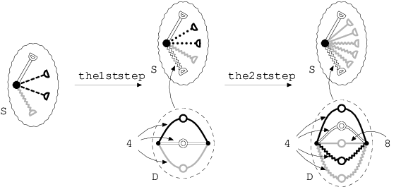
Dealing with Attached Edges and Loops. After the preprocessing step, the star atom contains several pendant edges, loops, half-edge attached to , with at most one half-edge corresponding to a dipole. If this dipole contains some non-halvable edges, then they are paired in every half-quotient and form loops. So we can remove them from the dipole and attach the corresponding number of loops directly to in . After this step, the dipole contains only even number of halvable edges in each color class.
Each pendant edge corresponds to a block atom attached to . Each loop either corresponds to a proper atom, or a dipole. Similarly as before, we expand these dipoles, replacing them by several loops corresponding to their edges. After this expansion, each pendant edge/loop corresponds to exactly one pendant element of . But since their expansion is unique, they can be contained in lists of only one type of pendant elements. Therefore we can arbitrarily assign pendant elements and remove these pendant elements and loops from and the assigned pendant elements from .
The resulting star atom contains only half-edges and at most one half-edge corresponds to a dipole having only halvable edges corresponding to proper atoms. Hence the considered star atom decomposes into the half-edges corresponding to proper atoms and at most one half-edge corresponding to a halvable dipole .
Reduction to the V-Matching Problem. Suppose that contains a half-edge corresponding to a dipole , otherwise the half-quotient of is unique and we can easily match it using perfect matching in a bipartite graph, as described in the proof of Lemma 26. Let be the set of the remaining half-edges attached in corresponding to proper atoms. In each half-quotient of the dipole , we have color classes of even sizes. For each color class of an even size , we can choose an arbitrary number of loops and the corresponding number of half-edges . If we know these values and , we can just test existence of a perfect matching as described in Lemma 26. Since we do not know the values and , we need to solve a generalization of perfect matching called IV-Matching in which we are free to choose these values.
The input of IV-Matching gives a bipartite graph defined similarly as before. One part has a vertex per a pendant element and the other part has a vertex for each edge of and half-edge of . We put an edge between and , if a half-quotient of or the loop-quotient created by rotating two edges is in the list . We call the first case a half-incidence and the latter case a loop-incidence. Further, we add a half-incidence between and , if the half-edge is contained in the list .
We ask whether there exists a spanning subgraphs of , with each component of connectivity a path of length one or two, as follows. Each pendant element is in either half-incident to exactly one vertex in the other part, or it is loop-incident to exactly two edges of the same color class. Further, each edge and half-edge is incident in to exactly one pendant element. In what follows, we call an IV-subgraph of . See Figure 28 for an example, with several additional properties which we discuss now.
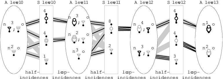
Special Properties of Inputs. The IV-Matching would likely be NP-complete in general, but there are additional properties already depicted in Figure 28. We describe them in details, since they might help in constructing a polynomial-time algorithm for this problem.
First, consists of separate connected components and for each we can solve the problem separately. A connected component is induced by a chain of pendant elements and its incident vertices representing . In what follows, we assume that we just have a single chain. This chain has its level structure which translates into a level structure for part with half-edges of and edges of as follows.
- •
Let be a half-edge of with and . Then this half-edge can be in half-incident to pendant elements only of the level with and .
- •
Let be an edge of the dipole with and . It can be half-incident to pendant elements only of the level with and and loop-incident to pendant elements only of the level with and .
So we also have levels for the other part of . Let us call these levels levels and levels, respectively. If we depict all levels from left to right according to their order, alternating levels of pendant elements levels and levels of half-edges of and edges of . The graph has only edges going between consecutive levels as depicted in Figure 28.
The second property says that can be viewed as a cluster graph. In each level, the edges of and the half-edges of form clusters according to their color classes. Similarly in each level, the pendant elements form clusters according to equivalence classes of their lists. (We note that two pendant elements with equal lists can correspond to non-isomorphic subgraphs in . Then their lists contain only half-edges.) Two clusters from different levels are either completely adjacent, or not adjacent at all. In other words, the subgraph induced by all edges between two clusters is either complete bipartite, or contains no edges.
Also each edge cluster is loop-adjacent to at most one pendant element cluster, since a loop-quotient contained in a list uniquely determines the pendant element, as discussed above. We do not need the condition that each list is loop-incident in the IV-subgraph to two edges of the same color class since this is automatically achieved. On the other hand, there are no constraints for half-incidences between clusters.
The third property reads as follows. If the highest level is an level, we can deal with this level greedily. All pendant elements of this level has to be loop-incident in , so we can ignore half-edges in their lists and assign them directly to the previous level. For instance in Figure 28, we know that we have two black shaken loops and one gray shaken loops. Therefore we can remove this level together with the corresponding number of edges of . We can assume that the highest level is an level. Similarly if the smallest level is an level, we can match it greedily. If the smallest level is an level, this greedy approach does not work. We know how many lists have to be realized by their half-quotients. But the lists may contain multiple half-edge colors and therefore may be realized by different edges of . Therefore in the next level we may end up with different numbers of edges of which may change solvability on higher levels.
Another property is that we know for each level of incidences, between two consecutive levels, how many edges have to be placed in . We can just process the graph from left to right. On the smallest level, we know how many half-incidences are in . Therefore we can compute the remaining number of edges of which are loop-incident in . By processing in this way from left to right, we get all the numbers. Notice that we do not know how many half- and loop-incidences are in for each cluster, otherwise we could solve the problem directly by a perfect matching in a modified graph.
Since the sizes of the levels are growing exponentially from left to right, we have at most logarithmically many levels with respect to the size of the graph . One can also show that the number of vertices in each level is somewhat limited by the size of the level, but it does not seem to give any useful bound.
6 Applying the Meta-algorithm to Planar Graphs
In this section, we show that the meta-algorithm described in Section 5 applies to the class of planar graphs. We describe the properties of planar graphs and their quotients in more details than necessary. We do it to give a deeper insight into regular covers of planar graphs.
6.1 Automorphism Groups of 3-connected Planar Graphs
We review the well-known properties of planar graphs and their automorphism groups. These strong properties are based on the Whitney’s Theorem [42] stating that a 3-connected graph has a unique embedding into the sphere.
Spherical Groups. A group is spherical if it is a group of symmetries of a tiling of the sphere. The first class of spherical groups are the subgroups of the automorphism groups of the platonic solids, i.e., for the tetrahedron, for the cube and the octahedron, and for the dodecahedron and the icosahedron. See Table 1 for the number of conjugacy classes of the subgroups of these three groups. Note that conjugate subgroups determine isomorphic quotients . The second class of spherical groups is formed by infinite families and .
| of the order 24 | |||
| Order | Number | Order | Number |
| 1 | 1 | 6 | 1 |
| 2 | 2 | 8 | 1 |
| 3 | 1 | 12 | 1 |
| 4 | 3 | ||
| of the order 48 | |||
| Order | Number | Order | Number |
| 1 | 1 | 8 | 7 |
| 2 | 5 | 12 | 2 |
| 3 | 1 | 16 | 1 |
| 4 | 9 | 24 | 3 |
| 6 | 3 | ||
| of the order 120 | |||
| Order | Number | Order | Number |
| 1 | 1 | 8 | 1 |
| 2 | 3 | 10 | 3 |
| 3 | 1 | 12 | 2 |
| 4 | 3 | 20 | 1 |
| 5 | 1 | 24 | 1 |
| 6 | 3 | 60 | 1 |
Automorphisms of a Map. A map is a 2-cell embedding of a graph onto a surface . For purpose of this paper, is either the sphere or the projective plane. A rotational scheme at a vertex is a cyclic ordering of the edges incident with the vertex. When working with abstract maps, they are graphs with a rotational scheme given for every vertex. An angle is a triple where is a vertex, and and are two incident edges which are consecutive in the rotational scheme of .
An automorphism of a map is an automorphism of the graph which preserves the angles; in other words the rotational scheme is preserved up to reflections. With the exception of paths and cycles, is a subgroup of . In general these two groups might be very different. For instance, the star has , but for any map of we just have .
Lemma 30
For any map , a permutation representation of the group can be computed in time where is the number of edges of .
Proof (Sketch)
There are angles in . We fix one angle , and test for each other angle whether there is an automorphism mapping to it. The key observation is that if such an automorphism exists, it is uniquely determined. We can just test in whether the map is compatible with this prescribed mapping. The total running time is .∎
If is drawn on the sphere, then is isomorphic to one of the spherical groups [23, 14]. In case is a -connected planar graph, there exists the unique embedding of onto the sphere. Then for any map of , we have [42]. Thus we get the following corollary of Lemma 30.
Corollary 7
If is a -connected planar graph, then is isomorphic to one of the spherical groups. We can determine this group in polynomial time and find permutations which generate it in time .
We note that a linear-time algorithm for computing automorphism groups of planar graphs is known [28].
6.2 Automorphisms and Quotients of Primitive Graphs and Atoms
To be able to apply the meta-theorem on planar graphs, we first investigate the automorphism groups of atoms and primitive graphs, and their quotients. Recall that a graph is essentially 3-connected if it is a 3-connected graph with attached single pendant edges.
Lemma 31
For a planar primitive graph , the group is a spherical group and can be computed in time .
Proof
For an atom , Recall that is the point-wise stabilizer of in . Further, by we denote the set-wise stabilizer of in .
Lemma 32
We get the following automorphism groups for atoms:
- •
For a star block atom, we get in general which is a direct product of symmetric groups.
- •
For a dipole, we get in general as a direct product of symmetric groups. For a symmetric dipole, we have , for non-symmetric .
- •
For a proper atom of a planar graph, the group is a subgroup of and is a subgroup of .
- •
For a non-star block atom of a planar graph, and it is a subgroup of .
Proof
The edges of the same color class of a star block atom can be arbitrary permuted, so we get for and the same group which is a direct product of symmetric groups. For a dipole the situation is similar, just for a symmetric dipole we can permute the vertices in , so we get a semidirect product with .
Let be a proper atom with , and let be the essentially 3-connected graph created by adding the edge . Since preserves , we have , and fixes in addition the edge . Because is essentially 3-connected, then corresponds to the stabilizer of in for the unique map of . But such a stabilizer has to be a subgroup of . For we further stabilize the vertices of , so it is a subgroup of .
Let be a non-star block atom. Then is preserved, so we have one fixed vertex in both and , so they are the same. Since is essentially 3-connected, then is a subgroup of where is the degree of .∎
As a corollary of Proposition 2, we can characterize automorphism groups of planar graphs, similarly to Babai [4, 5].
Corollary 8
Each automorphism group of a planar graph is obtained from a spherical groups by repeated semidirect products of direct products of groups of atoms from Lemma 32.
Proof
Geometry of Quotients. We review in more details the geometry of quotients of planar graphs. These are classical results from geometry of the sphere, and the reader can find the missing proofs and details in [41]. We note that this precise understanding is not necessary for the correctness of the meta-algorithm, but we believe it gives a deeper insight into the quotients of planar graphs, in the direction of the Negami’s Theorem [38].
We start by basic definitions from geometry. An automorphism of a 3-connected planar graph is called orientation preserving, if the respective map automorphism preserves the global orientation of the surface. It is called orientation reversing if it changes the global orientation of the surface. A group of automorphisms of a 3-connected planar graph is either orientation preserving, or it contains a subgroup of index two of orientation preserving automorphisms. (The reason is that composition of two orientation reversing automorphisms is an orientation preserving automorphism.)
Let be an orientation reversing involution. The involution is called antipodal if it is a semiregular automorphism of a closed orientable surface such that is a non-orientable surface. Otherwise is called a reflection. A reflection of the sphere fixes a circle.
In particular, the half-quotient of the sphere by an antipodal involution is the projective plane and the half-quotient by a reflection is a disk. An orientation reversing involution of a 3-connected planar graph is called antipodal if the respective map automorphism is antipodal and it is called a reflection if the respective map automorphism is a reflection. A reflection of a map on the sphere fixes always either an edge, or a vertex.
Lemma 33 ([41])
Let be a 3-connected planar graph and be a semiregular subgroup of . Then the following can happen:
- (a)
The action of is orientation preserving and the quotient is planar,
- (b)
The action of is orientation reversing but does not contain an antipodal involution. Then the quotient is planar and necessarily contains half-edges,
- (c)
The action of is orientation reversing and contains an antipodal involution. Then is projective planar.∎
As we show, if is projective non-planar, then necessarily also the quotient of associated primitive graph is projective non-planar. The reason is that a projection of an atom is always planar, and planarity is preserved by expansions.
Lemma 34
Let be a proper atom in planar graph and let . Then there are at most two involutory semiregular automorphisms transposing and . Moreover, if there are exactly two of them, then one is orientation preserving and the other one is a reflection. In particular, the two respective quotient graphs may be non-isomorphic planar graphs.
Proof
The graph is an essentially 3-connected planar graph with a unique embedding into the plane. Then any graph automorphism transposing and is a map automorphism fixing . It is easy to see that that either is a 180 degree rotation around the centre of , or it is a reflection [4, 5]. According to Lemma 33, both possible quotients are planar.∎
The following lemma is straightforward, and completes the description of possible quotients of primitive graphs.
Lemma 35
Let be a quotient of a cycle by a semiregular group of automorphisms. Then either is a cycle, or a path, or a path with one pendant half edge, or is a path with two pendant half edges. Depending on parity, just three of the above for cases happen.∎
6.3 The Class of Planar Graphs Satisfies (P0) to (P3)
In this section, we prove that planar graphs satisfy the properties (P0) to (P3), and thus the meta-algorithm of Section 5 applies to them. The class of planar graphs clearly satisfies (P0). The graph isomorphism can be tested in polynomial time for planar graphs [28] and for projective planar graphs [32], which implies (P1). For (P2), Corollary 7 states that the automorphism group of a 3-connected planar graph is a spherical group, and so we can generate all at most linearly many subgroups of given order and check which ones act semiregularly. It remains to prove (P3):
Proposition 4
The class of planar graphs satisfies the property (P3).
Proof
Let be a 3-connected projective planar graph. Lichtenstein [32] proved that there are two possible cases: Either the number of possible projective maps of is bounded by , or contains an edge such that is a planar graph. The property (P3) gives two 3-connected graphs and , and if , then necessarily (while ignoring the colors), and thus the same case happens for both and . We deal with these two cases separately.
Case 1: Linear number of projective maps. We want to show that the size of is polynomial in . To see this, every is either a map automorphism, or an isomorphism between two maps of . The number of automorphisms of a map is bounded by . Since we have a linear number of non-isomorphic maps, we get the bound , which is . We can construct all these automorphisms in polynomial time, for instance by attaching specific gadgets to the vertices of and , and testing whether the modified graphs are still isomorphic. Therefore we can compute in polynomial time, and by composition with some isomorphism from to , we can test whether there exists an embedding .
Case 2: Removal of two vertices makes each of the graphs and planar. We know that there exists and such that and are both planar graphs. We test possible choices of the pairs of vertices, and we want to test whether there exists an embedding such that and . Clearly, and . It remains to deal with the planar remainders and . Notice that and are not necessarily 3-connected.
Now, we can approach the problem exactly as with testing expandability of in the meta-algorithm. We code the colors of the vertices of by the colors of the single pendant edges attached to the corresponding vertices of , and we code the lists of the colors by the list of the pendant elements attached to the vertices in . We choose the central block/articulation of both and as the core.
First, we proceed with a series of reductions of , replacing the atoms by edges and placing them in the separate catalog. Here, the automorphisms are indeed color preserving. Further, we have four partition classes of according to the adjacencies to and , and automorphisms preserves them. We end up with a primitive 3-connected graph .
Using the constructed catalog, we proceed similarly with the reductions of . But there are two important differences. First, the starting graph already contains pendant elements with initial lists, given by . The second difference is that we have to remember lists also for interior edges of , not only for pendant elements. The reduction is done similarly, by replacing the atoms of by edges and pendant elements in . Let be an atom in , and to compute the list we iterate over all atoms of of the given type in the catalog. Let be one such atom from the catalog. Depending on the type of , we proceed as follows:
- •
If is a block atom of , then according to Lemma 32 we have is a subgroup of , and so we can test all possible isomorphisms from to . If one such isomorphism defines an embedding of to , we add the edge representing to the list.
- •
If is a proper atom of , then we similarly test according to Lemma 32 at most four possible isomorphisms from to .
- •
If is a dipole, we construct a bipartite graph. One part is formed by the colored edges of , the other part by the edges of with the associated lists of possible colors. The adjacencies are given by containments of the colors in the lists. We test existence of a perfect matching in this bipartite graph.
Finally, when we reach the primitive graph , then according to Lemma 31 we have that is a spherical group. Thus we can test all possible isomorphisms from to whether they are compatible with the lists of . The entire subroutine is clearly correct and runs in polynomial time.∎
7 Concluding Remarks
We conclude this paper by remarks to the meta-algorithm and open problems.
Possible Extensions of The Meta-algorithm. There are several possible natural extensions of the meta-algorithm. First, we can easily generalize it for input graph and with half-edges, directed edges and halvable edges, and also for colored graphs. Further, one can prescribe lists of possible images for the vertices and of possible pre-images of the vertices , the expandability testing can compute also with these lists.
The most interesting extension would be to use the meta-algorithm to generate all quotients of . Indeed, this cannot be achieved in polynomial time since there might be exponentially many such quotients. But we can enumerate all labeled quotients with a polynomial delay, by using different expansions determined in Proposition 3.
Open problems. We already discussed that RegularCover generalizes the graph isomorphism problem. We ask the following:
Problem 1
Is the problem RegularCover GI-complete?
Similarly to the graph isomorphism problem, we are given two graphs and which restrict each other. To solve RegularCover, one needs to understand automorphism groups of graphs and their semiregular subgroups.
As possible next direction of research, we suggest to attack classes of graphs close to planar graphs, for instance projective planar graphs or toroidal graphs. To do so, it seems that new techniques need to be built. Also the automorphism groups of projective planar graphs and toroidal graphs are not well understood.
Lastly, we indeed ask whether the slow subroutine for dipole expansion of the meta-algorithm can be solved in polynomial time:
Problem 2
Can the complexity of the algorithm of Theorem 1.1 be improved to be polynomial?
In Section 5.3, we have shown that the slow subroutine reduces to a generalized matching problem called IV-Matching. Here, we describe a purely combinatorial formulation of the IV-Matching problem. This reformulation can be useful to people studying combinatorial optimization since they can attack the problem without understanding the regular coverings and the structural results obtained in the entire paper.
The input of IV-Matching consists of a bipartite graph with a partitioning , with even, of its vertices which we call levels, with all edges between of consecutive levels and , for . The levels are called odd and the levels even. Further each level is partitioned into several clusters, each consisting of a few vertices with identical neighborhoods. There are three key properties:
- •
The incidences in respect the clusters; between any two clusters the graph induces either a complete bipartite graph, or an edge-less graph.
- •
Each cluster of an even level is incident with at most one cluster at the odd level , and each cluster of is incident with at most one cluster at ; so we have a matching between clusters at levels and .
- •
The incidences between the clusters of and can be arbitrary.
The problem IV-Matching asks whether there is a spanning subgraph with each component of connectivity equal to a path of length one or two. We call this subgraph an IV-subgraph of . Each vertex of an odd level is in adjacent either to exactly one vertex of , or to exactly two vertices of . Each vertex of an even level is adjacent to exactly one vertex of the levels . In other words, from to the edges of form a matching, not necessarily perfect. From to , the edges of form independent -shapes, with their centers in the level . Figure 29 shows an example.

Problem 3
What is the complexity of the IV-Matching problem?
It would be interesting to know solutions even to more restricted versions of this problem. For instance, what if the number of levels is small? We note that for instances having odd numbers of levels, as the one in Figure 29, we can match the highest level greedily; thus we can assume that the number of levels is always even. For two levels, the problem is just the standard perfect matching problem for bipartite graphs. On the other hand, already the case of four levels is very interesting and open. The instances of our algorithm needs to solve for the problem RegularCover have at most logarithmic number of levels in size of the smaller input graph .
References
- [1] S. B. Akers and B. Krishnamurthy. On group graphs and their fault tolerance. IEEE Trans. Comput., 36(7):885–888, 1987.
- [2] D. Angluin. Local and global properties in networks of processors. In ACM Symposium on Theory of Computing, pages 82–93. ACM, 1980.
- [3] D. Angluin and A. Gardiner. Finite common coverings of pairs of regular graphs. J. Combin. Theory Ser. B, 30(2):184–187, 1981.
- [4] L. Babai. Automorphism groups of planar graphs II. In Infinite and finite sets (Proc. Conf. Keszthely, Hungary, 1973) Bolyai-North-Holland, pages 29–84, 1975.
- [5] L. Babai. Automorphism groups, isomorphism, reconstruction. In Handbook of combinatorics (vol. 2), pages 1447–1540. MIT Press, 1996.
- [6] R. Bar-Yehuda and T. Etzion. Connections between two cycles – a new design of dense processor interconnection networks. Discrete Applied Mathematics, 37–38:29–43, 1992.
- [7] N. Biggs. Algebraic graph theory. Cambridge University Press, 1993.
- [8] O. Bílka, J. Jirásek, P. Klavík, M. Tancer, and J. Volec. On the complexity of planar covering of small graphs. In LNCS, WG, volume 6986, pages 83–94, 2011.
- [9] H. L. Bodlaender. The classification of coverings of processor networks. Journal of Parallel and Distributed Computing, 6(1):166–182, 1989.
- [10] L. Campbell. Dense group networks. Discrete Applied Mathematics, 37–38:65–71, 1992.
- [11] L. Campbell, G. E. Carlsson, M. J. Dinneen, V. Faber, M. R. Fellows, M. A. Langston, J. W. Moore, A. P. Mullhaupt, and H. B. Sexton. Small diameter symmetric networks from linear groups. IEEE Trans. Comput., 41(2):218–220, 1992.
- [12] G. E. Carlsson, J. E. Cruthirds, H. B. Sexton, and C. G. Wright. Interconnection networks based on a generalization of cube-connected cycles. IEEE Trans. Comput., 100(8):769–772, 1985.
- [13] A. Cayley. The theory of groups: Graphical representation. Amer. J. Math., 1:174–176, 1878.
- [14] H. S. M. Coxeter. Introduction to geometry. New York, London, 1961.
- [15] P. Erdös, S. Fajtlowicz, and A. J. Hoffman. Maximum degree in graphs of diameter 2. Networks, 10(1):87–90, 1980.
- [16] S. Evdokimov and I. Ponomarenko. Circulant graphs: recognizing and isomorphism testing in polynomial time. St. Petersburg Mathematical Journal, 15(6):813–835, 2004.
- [17] H. M. Farkas and I. Kra. Riemann surfaces. In Riemann Surfaces, volume 71 of Graduate Texts in Mathematics, pages 9–31. 1992.
- [18] T. Feder and M. Y. Vardi. The computational structure of monotone monadic snp and constraint satisfaction: A study through datalog and group theory. SIAM Journal on Computing, 28(1):57–104, 1998.
- [19] M. R. Fellows and J. C. Stillweil. On the complexity and combinatorics of covering finite complexes. Australasian Journal of Combinatorics, 4:103–112, 1991.
- [20] J. Fiala. Note on the computational complexity of covering regular graphs. In 9th Annual Conference of Doctoral Students, WDS’00, pages 89–90. Matfyzpress, 2000.
- [21] J. Fiala and J. Kratochvíl. Locally constrained graph homomorphisms—structure, complexity, and applications. Computer Science Review, 2(2):97–111, 2008.
- [22] D. M. Goldschmidt. Automorphisms of trivalent graphs. Annals of Mathematics, 111(2):377–406, 1980.
- [23] J. L. Gross and T. W. Tucker. Topological graph theory. Courier Dover Publications, 2001.
- [24] D. Guo, J. Wu, H. Chen, and X. Luo. Moore: An extendable peer-to-peer network based on incomplete Kautz digraph with constant degree. In INFOCOM 2007. 26th IEEE International Conference on Computer Communications. IEEE, pages 821–829, 2007.
- [25] Z. Hedrlín and A. Pultr. On full embeddings of categories of algebras. Illinois Journal of Mathematics, 10(3):392–406, 1966.
- [26] P. Hell and J. Nešetřil. On the complexity of -coloring. J. Combin. Theory Ser. B, 48(1):92–110, 1990.
- [27] A. J. Hoffman and R. R. Singleton. On moore graphs with diameters 2 and 3. IBM Journal of Research and Development, 4(5):497–504, 1960.
- [28] J. E. Hopcroft and R. E. Tarjan. Isomorphism of planar graphs. In Complexity of computer computations, pages 131–152. Springer, 1972.
- [29] J. E. Hopcroft and R. E. Tarjan. Dividing a graph into triconnected components. SIAM Journal on Computing, 2(3):135–158, 1973.
- [30] M. O. Katanaev. All universal coverings of two-dimensional gravity with torsion. Journal of mathematical physics, 34:700–736, 1993.
- [31] J. Kratochvíl, A. Proskurowski, and J. A. Telle. Covering regular graphs. J. Comb. Theory Ser. B, 71(1):1–16, 1997.
- [32] D. Lichtenstein. Isomorphism for graphs embeddable on the projective plane. In ACM Symposium on Theory of Computing, STOC ’80, pages 218–224, 1980.
- [33] A. Lubiw. Some NP-complete problems similar to graph isomorphism. SIAM Journal on Computing, 10(1):11–21, 1981.
- [34] A. Malnič, R. Nedela, and M. Škoviera. Lifting graph automorphisms by voltage assignments. European Journal of Combinatorics, 21(7):927–947, 2000.
- [35] Rudolf Mathon. A note on the graph isomorphism counting problem. Information Processing Letters, 8(3):131–132, 1979.
- [36] B. D. McKay, M. Miller, and J. Širáň. A note on large graphs of diameter two and given maximum degree. J. Combin. Theory Ser. B, 74(1):110–118, 1998.
- [37] M. Miller and J. Širáň. Moore graphs and beyond: A survey of the degree/diameter problem. Electronic Journal of Combinatorics, 61:1–63, 2005.
- [38] S. Negami. The spherical genus and virtually planar graphs. Discrete Mathematics, 70(2):159–168, 1988.
- [39] G. Ringel and J. Youngs. Solution of the Heawood map-coloring problem. Proceedings of the National Academy of Sciences of the United States of America, 60(2):438–445, 1968.
- [40] J.J. Rotman. An Introduction to the Theory of Groups. Graduate Texts in Mathematics. Springer, 1994.
- [41] J. Stillwell. Geometry of surfaces. Springer, 1992.
- [42] H. Whitney. Nonseparable and planar graphs. Trans. Amer. Math. Soc., 34:339–362, 1932.
- [43] S. Zhou. A class of arc-transitive Cayley graphs as models for interconnection networks. SIAM Journal on Discrete Mathematics, 23(2):694–714, 2009.