跳到论文正文
W Papers独立论文阅读器 arXiv:1402.3710 论文正文 计算阅读时间 · 0%
引用这篇论文根据当前论文元数据生成,正式投稿前建议核对。


License: arXiv.org perpetual non-exclusive license
arXiv:1402.3710v2 [math.FA] 05 Sep 2014

Multivariate periodic wavelets of de la Vallée Poussin type

Ronny Bergmann ††thanks: Department of Mathematics, University of Technology Kaiserslautern, Paul-Ehrlich-Straße 31, D-67653 Kaiserslautern, Germany, bergmann@mathematik.uni-kl.de    Jürgen Prestin ††thanks: Institute of Mathematics, University of Lübeck, Ratzeburger Allee 160, D-23562 Lübeck, Germany.
prestin@math.uni-luebeck.de
Abstract

In this paper we present a general approach to multivariate periodic wavelets generated by scaling functions of de la Vallée Poussin type. These scaling functions and their corresponding wavelets are determined by their Fourier coefficients, which are sample values of a function, that can be chosen arbitrarily smooth, even with different smoothness in each direction. This construction generalizes the one-dimensional de la Vallée Poussin means to the multivariate case and enables the construction of wavelet systems, where the set of dilation matrices for the two-scale relation of two spaces of the multiresolution analysis may contain shear and rotation matrices. It further enables the functions contained in each of the function spaces from the corresponding series of scaling spaces to have a certain direction or set of directions as their focus, which is illustrated by detecting jumps of certain directional derivatives of higher order.

Keywords.

wavelets, lattices, de la Vallée Poussin means, periodic multiresolution analysis, shift-invariant space

Mathematical Subject Classification 2010.

42C40, 65T60

1 Introduction

In the recent years, a framework for multivariate wavelets was developed [1, 7, 9, 10, 11, 14], generalizing the one-dimensional periodic wavelets, which were developed in [13, 14, 16], to the multivariate case. By introducing the possibility to use any integer matrix for the underlying patterns, this framework possesses anisotropic approximation properties [4]. The directional approach was also discussed in the case of wavelets on the ℝd\mathbb{R}^{d} recently, e.g. for the shearlets [6] in order to detect singularities [8]. For the one-dimensional case the de la Vallée Poussin means and their corresponding periodic wavelets create a multiresolution analysis (MRA) with a fast decomposition algorithm and provide good localization [17, 18]. These de la Vallée Poussin wavelets were used in [12] in order to detect singularities of a function. In [10] an MRA was constructed using Dirichlet kernels and a certain set of dilation matrices. In [1] fast algorithms for both the Fourier and wavelet transform were presented for any set of dilation matrices and corresponding scaling functions forming an MRA.

Our main goal is the construction of multivariate trigonometric functions defined through their Fourier coefficients by sampling a function gg of certain smoothness. This function gg can be of compact support and the sampling points vary for each space of the nested sequence of spaces that form the MRA. We investigate, how to also obtain the coefficients of the two-scale relation from this construction. For a special case, gg resembles not only the de la Vallée Poussin means of the one-dimensional case, but also the mentioned Dirichlet kernels. Choosing a smooth function gg follows the idea of obtaining well localized scaling functions which also lead to well localized periodic wavelets. This construction further introduces the possibility to use arbitrary dilation matrices, especially shearing matrices such as 𝐉X±:=(20±11)\mathbf{J}_{\text{X}}^{\pm}:=\bigl(\begin{smallmatrix}2&0\\ \pm 1&1\end{smallmatrix}\bigr) and 𝐉Y±:=(1±102)\mathbf{J}_{\text{Y}}^{\pm}:=\bigl(\begin{smallmatrix}1&\pm 1\\ 0&2\end{smallmatrix}\bigr). The presented approach does not only enable a construction for an arbitrary set of scaling functions, for the dyadic case we also obtain a similar construction for the corresponding wavelets. Their analogues to the two-scale relation, i.e. the coefficients that characterize the wavelet in the scaling space they are nested in, is derived. Both, the two-scale relation and these coefficients can be computed just using gg and the dilation matrix 𝐉\mathbf{J} involved.

We investigate for which functions gg we can derive a construction of a set of nested dyadic spaces where each scaling function φj\varphi_{j} together with its translates forms a basis for the corresponding space and depends on the next scaling function φj+1\varphi_{j+1} at most. On the one hand, the construction enables an explicit description of a complete MRA using the function gg. On the other hand, it increases the flexibility of an adaptive MRA, where the sequence of dilation matrices 𝐉j\mathbf{J}_{j} and hence their scaling functions φj\varphi_{j} and wavelets ψj\psi_{j} can be chosen adaptively. The scaling spaces obtained in this setting can also be used to construct and characterize anisotropic interpolation operators. Corresponding error estimates and function spaces are discussed in [4].

The remainder of this paper is organized as follows. In Section 2 we first introduce basic preliminaries in order to define the multiresolution analysis for an arbitrary sequence of dilation matrices {𝐉j}j>0\{\mathbf{J}_{j}\}_{j>0}. For the dyadic case, i.e. where |det𝐉j|=2|\det\mathbf{J}_{j}|=2 for all j>0j>0, Lemma 2.2 characterizes the orthonormality of the translates of the corresponding wavelet. In Lemmata 2.4-2.7 the MRA is described, by using the Fourier coefficients c𝐤​(φj)c_{\mathbf{k}}(\varphi_{j}) of the scaling functions φj\varphi_{j}.

In Section 3 we introduce the notation of the classical de la Vallée Poussin means from [17, 18] and refine its notation in order to demonstrate the challenges arising by building a direct multivariate analogue.

The functions of de la Vallée Poussin type based on a smooth function gg are presented in Section 4. For a sequence of nn dilation matrices we obtain n+1n+1 scaling functions. The spaces of their translates are characterized in Theorem 4.3, especially the spaces are nested and the Fourier coefficients of these scaling functions are sample values of a function that possesses the same smoothness properties as gg. For the dyadic case, i.e. both the scaling space corresponding to jj and its orthogonal complement with respect to the next space j+1j+1 are again a spaces of translates of just one function each, we obtain a wavelet of de la Vallée Poussin type, which is investigated in Theorem 4.6. It inherits the properties from the corresponding scaling functions and is also given through Fourier coefficients by sampling a smooth function, too.

Finally, in Section 5 we investigate for which functions gg the dyadic scaling functions φ𝐌l𝒥l+1,n\varphi_{\mathbf{M}_{l}}^{\mathcal{J}_{l+1,n}} do not depend on the complete vector of matrices 𝒥l+1,n\mathcal{J}_{l+1,n}, but only on the first matrix 𝐉l+1\mathbf{J}_{l+1}. This generalizes the one-dimensional case, where only the scaling factor 22 was fixed. Starting from the two-dimensional case, we also investigate the dd-dimensional case. Finally, in Section 6 the wavelets of de la Vallée Poussin type are illustrated by decomposing a two-dimensional box spline with two specific wavelets in order to detect singularities of its higher order directional derivatives.

2 The multiresolution analysis

For a regular matrix 𝐌∈ℤd×d\mathbf{M}\in\mathbb{Z}^{d\times d}, d∈ℕd\in\mathbb{N}, we define the lattice Λ⁡(𝐌):=𝐌−1​ℤd\Lambda(\mathbf{M}):=\mathbf{M}^{-1}\mathbb{Z}^{d} and obtain an equivalence relation with respect to mod𝟏\bmod\mathbf{1} on Λ⁡(𝐌)\Lambda(\mathbf{M}), where 𝟏\mathbf{1} denotes the vector (1,…,1)T∈ℝd(1,\ldots,1)^{\mathrm{T}}\in\mathbb{R}^{d}. For a vector 𝐱∈ℝd\mathbf{x}\in\mathbb{R}^{d} we denote the usual Euclidean norm by ‖𝐱‖\|\mathbf{x}\|. A pattern 𝒫​(𝐌)\mathcal{P}_{\!\mathrm{}}(\mathbf{M}) is defined as any set of representatives ofmod𝟏\bmod\mathbf{1} on the lattice Λ⁡(𝐌)\Lambda(\mathbf{M}). Any pattern 𝒫​(𝐌)\mathcal{P}_{\!\mathrm{}}(\mathbf{M}) equipped with the addition mod𝟏\bmod\mathbf{1} generates an abelian group. Especially with 𝒬d:=[−12,12)d\mathcal{Q}_{d}:=\bigl[-\tfrac{1}{2},\tfrac{1}{2}\bigr)^{d} the two sets

𝒫S(𝐌):=𝐌−1ℤd∩𝒬d and 𝒫I(𝐌):=𝐌−1ℤd∩[0,1)d\mathcal{P}_{\!\mathrm{S}}(\mathbf{M}):=\mathbf{M}^{-1}\mathbb{Z}^{d}\cap\mathcal{Q}_{d}\quad\text{ and }\quad\mathcal{P}_{\!\mathrm{I}}(\mathbf{M}):=\mathbf{M}^{-1}\mathbb{Z}^{d}\cap[0,1)^{d}

are patterns. In the following we will omit the notation mod𝟏\bmod\mathbf{1}, wherever it is clear from the context, that the addition of two elements 𝐱+𝐲\mathbf{x}+\mathbf{y} of a pattern is performed.

For a multivariate 2​π2\pi-periodic function f:𝕋d→ℝf:\mathbb{T}^{d}\to\mathbb{R}, where 𝕋d:=ℝd/2​π​ℤd\mathbb{T}^{d}:=\mathbb{R}^{d}/2\pi\mathbb{Z}^{d} denotes the dd-dimensional torus, we can apply the shift operator T𝐲f:=f(∘−2π𝐲)\text{T}_{\mathbf{y}}f:=f(\circ-2\pi\mathbf{y}), 𝐲∈ℝd\mathbf{y}\in\mathbb{R}^{d}.

For any factorization 𝐌=𝐉𝐍\mathbf{M}=\mathbf{J}\mathbf{N}, the pattern 𝒫X​(𝐍)\mathcal{P}_{\!X}(\mathbf{N}) is a subset of 𝒫X​(𝐌)\mathcal{P}_{\!X}(\mathbf{M}), X∈{S,I}X\in\{\text{S},\text{I}\}. For this factorization we use the same notation for any set of representatives, i.e. 𝒫​(𝐍)⊂𝒫​(𝐌)\mathcal{P}_{\!\mathrm{}}(\mathbf{N})\subset\mathcal{P}_{\!\mathrm{}}(\mathbf{M}). Using the congruence relation on ℤd\mathbb{Z}^{d} with respect to a regular matrix 𝐌∈ℤd×d\mathbf{M}\in\mathbb{Z}^{d\times d}, which is defined by

𝐡≡𝐤mod𝐌⇔∃𝐳∈ℤd×d:𝐤=𝐡+𝐌T​𝐳,𝐤,𝐡∈ℤd​,\mathbf{h}\equiv\mathbf{k}\bmod\mathbf{M}\Leftrightarrow\exists\,\mathbf{z}\in\mathbb{Z}^{d\times d}:\mathbf{k}=\mathbf{h}+\mathbf{M}^{\mathrm{T}}\mathbf{z},\quad\mathbf{k},\mathbf{h}\in\mathbb{Z}^{d}\text{,}

we further define the generating set 𝒢​(𝐌)\mathcal{G}_{\mathrm{}}(\mathbf{M}) as any set of congruence representants of the equivalence relation mod𝐌\bmod\mathbf{M}. Due to the bijectivity of the linear map 𝐌∘\mathbf{M}\circ, a pattern always derives a generating set 𝒢​(𝐌)=𝐌​𝒫​(𝐌)\mathcal{G}_{\mathrm{}}(\mathbf{M})=\mathbf{M}\mathcal{P}_{\!\mathrm{}}(\mathbf{M}), in particular

𝒢S(𝐌):=ℤd∩𝐌𝒬d and 𝒢I(𝐌):=ℤd∩𝐌[0,1)d\mathcal{G}_{\mathrm{S}}(\mathbf{M}):=\mathbb{Z}^{d}\cap\mathbf{M}\mathcal{Q}_{d}\quad\text{ and }\quad\mathcal{G}_{\mathrm{I}}(\mathbf{M}):=\mathbb{Z}^{d}\cap\mathbf{M}[0,1)^{d}

are generating sets. When performing additions on the generating set 𝒢⁡(𝐌)\mathcal{G}(\mathbf{M}), i.e. with respect to mod𝐌\bmod\mathbf{M}, we omit the modulo, when it is clear from the context, that the result is again an element from 𝒢⁡(𝐌)\mathcal{G}(\mathbf{M}). Using a geometrical argument [5, Lemma II.7], it holds

|𝒫​(𝐌)|=|𝒫​(𝐌T)|=|𝒢​(𝐌)|=|𝒢​(𝐌T)|=|det𝐌|=:m​.|\mathcal{P}_{\!\mathrm{}}(\mathbf{M})|=|\mathcal{P}_{\!\mathrm{}}(\mathbf{M}^{\mathrm{T}})|=|\mathcal{G}_{\mathrm{}}(\mathbf{M})|=|\mathcal{G}_{\mathrm{}}(\mathbf{M}^{\mathrm{T}})|=|\det\mathbf{M}|=:m\text{.}

For any regular matrix 𝐌∈ℤd×d\mathbf{M}\in\mathbb{Z}^{d\times d} the Fourier matrix ℱ⁡(𝐌)\mathcal{F}(\mathbf{M}) is given by

ℱ⁡(𝐌):=1m​(e−2​π​i​𝐡T​𝐲)𝐡∈𝒢​(𝐌T),𝐲∈𝒫​(𝐌)∈ℂm×m​,\mathcal{F}(\mathbf{M}):=\frac{1}{\sqrt{m}}\left(\mathrm{e}^{-2\pi\mathrm{i}\mathbf{h}^{\mathrm{T}}\mathbf{y}}\right)_{\mathbf{h}\in\mathcal{G}_{\mathrm{}}(\mathbf{M}^{\mathrm{T}}),\mathbf{y}\in\mathcal{P}_{\!\mathrm{}}(\mathbf{M})}\in\mathbb{C}^{m\times m}\text{,} (1)

where the pattern 𝒫​(𝐌)\mathcal{P}_{\!\mathrm{}}(\mathbf{M}) addressing the columns and the generating set 𝒢​(𝐌)\mathcal{G}_{\mathrm{}}(\mathbf{M}) addressing the rows are ordered in an arbitrary but fixed way. For any vector 𝐚=(a𝐲)𝐲∈𝒫​(𝐌)\mathbf{a}=\bigl(a_{\mathbf{y}}\bigr)_{\mathbf{y}\in\mathcal{P}_{\!\mathrm{}}(\mathbf{M})} having the same order as the columns of the Fourier matrix ℱ⁡(𝐌)\mathcal{F}(\mathbf{M}) the discrete Fourier transform with respect to 𝐌\mathbf{M} is defined by

𝐚^:=(a^𝐡)𝐡∈𝒢​(𝐌T)=m​ℱ​(𝐌)​𝐚∈ℂm​,\mathbf{\hat{a}}:=(\hat{a}_{\mathbf{h}})_{\mathbf{h}\in\mathcal{G}_{\mathrm{}}(\mathbf{M}^{\mathrm{T}})}=\sqrt{m}\mathcal{F}(\mathbf{M})\mathbf{a}\in\mathbb{C}^{m}\text{,}

where 𝐚^=(a𝐡)𝐡∈𝒢​(𝐌T)\mathbf{\hat{a}}=(a_{\mathbf{h}})_{\mathbf{h}\in\mathcal{G}_{\mathrm{}}(\mathbf{M}^{\mathrm{T}})} has the same order of the elements as the rows of ℱ⁡(𝐌)\mathcal{F}(\mathbf{M}). For a certain order of the elements of both sets, a fast Fourier transform exists [1, Section 4].

A subspace VV of functions of the Hilbert space L2​(𝕋d)L_{2}(\mathbb{T}^{d}) on the torus 𝕋d\mathbb{T}^{d} is called shift-invariant with respect to 𝐌\mathbf{M}, or 𝐌\mathbf{M}-invariant, if

∀φ∈V,𝐲∈𝒫(𝐌):T𝐲φ:=φ(∘−2π𝐲)∈V.\forall\varphi\in V,\ \mathbf{y}\in\mathcal{P}_{\!\mathrm{}}(\mathbf{M})\,:\,\text{T}_{\mathbf{y}}\varphi:=\varphi(\circ-2\pi\mathbf{y})\in V\text{.}

An important example of an 𝐌\mathbf{M}-invariant space is given by the span of translates of φ∈L2​(𝕋d)\varphi\in L_{2}(\mathbb{T}^{d}), i.e.

V𝐌φ:=span⁡{T𝐲​φ:𝐲∈𝒫​(𝐌)}​,V_{\mathbf{M}}^{\,\varphi}:=\operatorname{span}\bigl\{\text{T}_{\mathbf{y}}\varphi\,:\,\mathbf{y}\in\mathcal{P}_{\!\mathrm{}}(\mathbf{M})\bigr\}\text{,}

where each function f∈V𝐌φf\in V_{\mathbf{M}}^{\,\varphi} can be written as

f=∑𝐲∈𝒫​(𝐌)a𝐲​T𝐲​φ,a𝐲∈ℂ​.f=\sum_{\mathbf{y}\in\mathcal{P}_{\!\mathrm{}}(\mathbf{M})}a_{\mathbf{y}}\text{T}_{\mathbf{y}}\varphi,\quad a_{\mathbf{y}}\in\mathbb{C}\text{.} (2)

This can also be equivalently formulated using the scalar product of the Hilbert space L2​(𝕋d)L_{2}(\mathbb{T}^{d}), the Fourier coefficients

c𝐤(φ):=⟨φ,ei𝐤T∘⟩=1(2​π)d∫𝕋dφ(𝐱)ei​𝐤T​𝐱d𝐱,𝐤∈ℤd,c_{\mathbf{k}}(\varphi):=\langle\varphi,\mathrm{e}^{\mathrm{i}\mathbf{k}^{\mathrm{T}}\circ}\rangle=\frac{1}{(2\pi)^{d}}\int_{\mathbb{T}^{d}}\varphi(\mathbf{x})\mathrm{e}^{\mathrm{i}\mathbf{k}^{\mathrm{T}}\mathbf{x}}\,\mathrm{d}\mathbf{x},\quad\mathbf{k}\in\mathbb{Z}^{d}\text{,}

and the Parseval equation, as [10, Theorem 3.3]

c𝐡+𝐌T​𝐳​(f)=a^𝐡​c𝐡+𝐌T​𝐳​(φ) holds for all ​𝐡∈𝒢​(𝐌),𝐳∈ℤd​,c_{\mathbf{h}+\mathbf{M}^{\mathrm{T}}\mathbf{z}}(f)=\hat{a}_{\mathbf{h}}c_{\mathbf{h}+\mathbf{M}^{\mathrm{T}}\mathbf{z}}(\varphi)\quad\text{ holds for all }\mathbf{h}\in\mathcal{G}_{\mathrm{}}(\mathbf{M}),\mathbf{z}\in\mathbb{Z}^{d}\text{,} (3)

where 𝐚^=(a^𝐡)𝐡∈𝒢​(𝐌T)\mathbf{\hat{a}}=(\hat{a}_{\mathbf{h}})_{\mathbf{h}\in\mathcal{G}_{\mathrm{}}(\mathbf{M}^{\mathrm{T}})} is the discrete Fourier transform of a vector of coefficients 𝐚=(a𝐲)𝐲∈𝒫​(𝐌)\mathbf{a}=(a_{\mathbf{y}})_{\mathbf{y}\in\mathcal{P}_{\!\mathrm{}}(\mathbf{M})} from (2).

For any factorization 𝐌=𝐉𝐍\mathbf{M}=\mathbf{J}\mathbf{N} the sub-pattern 𝒫​(𝐍)\mathcal{P}_{\!\mathrm{}}(\mathbf{N}) also induces a subspace, i.e. for a function η∈V𝐌φ\eta\in V_{\mathbf{M}}^{\varphi} we obtain V𝐍η⊂V𝐌φV_{\mathbf{N}}^{\,\eta}\subset V_{\mathbf{M}}^{\,\varphi}. Using the coefficients characterizing η\eta with respect to the translates of φ\varphi, cf. [10, Lemma 4.2 (i) and (ii)], we can characterize each function f∈V𝐍ηf\in V_{\mathbf{N}}^{\,\eta} also in V𝐌φV_{\mathbf{M}}^{\varphi}. We extend this characterization by the following Lemma to investigate the orthogonality of the translates T𝐱​η\text{T}_{\mathbf{x}}\eta, 𝐱∈𝒫​(𝐍)\mathbf{x}\in\mathcal{P}_{\!\mathrm{}}(\mathbf{N}), of the subspace.

Lemma 2.1.

Let 𝐌=𝐉𝐍\mathbf{M}=\mathbf{J}\mathbf{N} and a function φ∈L2​(𝕋d)\varphi\in L_{2}(\mathbb{T}^{d}) be given, such that the shifts T𝐲​φ\text{T}_{\mathbf{y}}\varphi, 𝐲∈𝒫​(𝐌)\mathbf{y}\in\mathcal{P}_{\!\mathrm{}}(\mathbf{M}), are an orthonormal basis of the 𝐌\mathbf{M}-invariant space V𝐌φV_{\mathbf{M}}^{\,\varphi}. Let η=∑𝐲∈𝒫​(𝐌)b𝐲​T𝐲​φ∈V𝐌φ\eta=\sum_{\mathbf{y}\in\mathcal{P}_{\!\mathrm{}}(\mathbf{M})}b_{\mathbf{y}}\text{T}_{\mathbf{y}}\varphi\in V_{\mathbf{M}}^{\,\varphi} be given. Then the translates T𝐱​η\text{T}_{\mathbf{x}}\eta, 𝐱∈𝒫​(𝐍)\mathbf{x}\in\mathcal{P}_{\!\mathrm{}}(\mathbf{N}), are orthonormal if and only if

∑𝐠∈𝒢​(𝐉T)|b^𝐤+𝐍T​𝐠|2=|det𝐉| holds for all ​𝐤∈𝒢​(𝐍T)​,\sum_{\mathbf{g}\in\mathcal{G}_{\mathrm{}}(\mathbf{J}^{\mathrm{T}})}|\hat{b}_{\mathbf{k}+\mathbf{N}^{\mathrm{T}}\mathbf{g}}|^{2}=|\det\mathbf{J}|\quad\text{ holds for all }\mathbf{k}\in\mathcal{G}_{\mathrm{}}(\mathbf{N}^{\mathrm{T}})\text{,}

where 𝐛^\mathbf{\hat{b}} is the discrete Fourier Transform of 𝐛=(b𝐲)𝐲∈𝒫​(𝐌)\mathbf{b}=\bigl(b_{\mathbf{y}}\bigr)_{\mathbf{y}\in\mathcal{P}_{\!\mathrm{}}(\mathbf{M})}.

Proof.

Let m=|det𝐌|m=\lvert\det\mathbf{M}\rvert and n=|det𝐍|n=\lvert\det\mathbf{N}\rvert. Using [10, Corollary 3.6], (3) and the orthonormality of the translates T𝐲​φ\text{T}_{\mathbf{y}}\varphi, 𝐲∈𝒫​(𝐌)\mathbf{y}\in\mathcal{P}_{\!\mathrm{}}(\mathbf{M}), the orthonormality of the translates T𝐱​η\text{T}_{\mathbf{x}}\eta, 𝐱∈𝒫​(𝐍)\mathbf{x}\in\mathcal{P}_{\!\mathrm{}}(\mathbf{N}), η∈V𝐌φ\eta\in V_{\mathbf{M}}^{\,\varphi} as above, is equivalent to the fact that it holds for all 𝐤∈𝒢​(𝐍T)\mathbf{k}\in\mathcal{G}_{\mathrm{}}(\mathbf{N}^{\mathrm{T}})

|det𝐉|=mn\displaystyle|\det{\mathbf{J}}|=\frac{m}{n} =m​∑𝐰∈ℤd|c𝐤+𝐍T​𝐰​(η)|2\displaystyle=m\sum_{\mathbf{w}\in\mathbb{Z}^{d}}|c_{\mathbf{k}+\mathbf{N}^{\mathrm{T}}\mathbf{w}}(\eta)|^{2}
=m​∑𝐠∈𝒢​(𝐉T)|b^𝐤+𝐍T​𝐠|2​∑𝐳∈ℤd|c𝐤+𝐍T​𝐠+𝐌T​𝐳​(η)|2\displaystyle=m\sum_{\mathbf{g}\in\mathcal{G}_{\mathrm{}}(\mathbf{J}^{\mathrm{T}})}|\hat{b}_{\mathbf{k}+\mathbf{N}^{\mathrm{T}}\mathbf{g}}|^{2}\sum_{\mathbf{z}\in\mathbb{Z}^{d}}|c_{\mathbf{k}+\mathbf{N}^{\mathrm{T}}\mathbf{g}+\mathbf{M}^{\mathrm{T}}\mathbf{z}}(\eta)|^{2}
=∑𝐠∈𝒢​(𝐉T)|b^𝐤+𝐍T​𝐠|2​.∎\displaystyle=\sum_{\mathbf{g}\in\mathcal{G}_{\mathrm{}}(\mathbf{J}^{\mathrm{T}})}|\hat{b}_{\mathbf{k}+\mathbf{N}^{\mathrm{T}}\mathbf{g}}|^{2}\text{.}\qed

If f∈V𝐌φf\in V_{\mathbf{M}}^{\,\varphi} is known by its coefficient vector 𝐚∈ℂm\mathbf{a}\in\mathbb{C}^{m} from (2) , then the projection f𝐍,ηf_{\mathbf{N},\eta} of ff onto V𝐍ηV_{\mathbf{N}}^{\,\eta} is given in matrix form in [10, Lemma 4.2 (iii)] and can be reformulated as [3, (1.50)]

d^𝐤=1|det𝐉|​∑𝐠∈𝒢​(𝐉T)a^𝐤+𝐍T​𝐠¯​b^𝐤+𝐍T​𝐠​,𝐤∈𝒢​(𝐍T)​,\hat{d}_{\mathbf{k}}=\frac{1}{\sqrt{|\det{\mathbf{J}}|}}\sum_{\mathbf{g}\in\mathcal{G}_{\mathrm{}}(\mathbf{J}^{\mathrm{T}})}\overline{\hat{a}_{\mathbf{k+\mathbf{N}^{\mathrm{T}}\mathbf{g}}}}\hat{b}_{\mathbf{k}+\mathbf{N}^{\mathrm{T}}\mathbf{g}}\text{,}\quad\mathbf{k}\in\mathcal{G}_{\mathrm{}}(\mathbf{N}^{\mathrm{T}})\text{,} (4)

such that f𝐍,η=∑𝐱∈𝒫​(𝐍)d𝐱​T𝐱​ηf_{\mathbf{N},\eta}=\sum_{\mathbf{x}\in\mathcal{P}_{\!\mathrm{}}(\mathbf{N})}d_{\mathbf{x}}\text{T}_{\mathbf{x}}\eta, where again 𝐝^∈ℂn\mathbf{\hat{d}}\in\mathbb{C}^{n} is the discrete Fourier transform (with respect to 𝐍\mathbf{N}) of 𝐝∈ℂn\mathbf{d}\in\mathbb{C}^{n}.

Let the translates T𝐲​φ\text{T}_{\mathbf{y}}\varphi, 𝐲∈𝒫​(𝐌)\mathbf{y}\in\mathcal{P}_{\!\mathrm{}}(\mathbf{M}), be linearly independent. Let further a set of functions η1,…,η|det𝐉|∈V𝐌φ\eta_{1},\ldots,\eta_{|\det{\mathbf{J}}|}\in V_{\mathbf{M}}^{\varphi} be given such that the translates T𝐱​ηj\text{T}_{\mathbf{x}}\eta_{j} are linearly independent for each j=1,…,|det𝐉|j=1,\ldots,|\det\mathbf{J}|. If these translates are mutually orthogonal, i.e. ⟨T𝐱​ηi,T𝐲​ηj⟩=0\langle\text{T}_{\mathbf{x}}\eta_{i},\text{T}_{\mathbf{y}}\eta_{j}\rangle=0 for each i≠ji\neq j, i,j∈{1,…,|det𝐉|}i,j\in\{1,\ldots,|\det\mathbf{J}|\}, and 𝐱≠𝐲\mathbf{x}\neq\mathbf{y}, 𝐱,𝐲∈𝒫​(𝐍)\mathbf{x},\mathbf{y}\in\mathcal{P}_{\!\mathrm{}}(\mathbf{N}), we obtain an orthogonal decomposition of the space V𝐌φV_{\mathbf{M}}^{\,\varphi} into

V𝐌φ=⨁j=1|det𝐉|V𝐍ηj​.V_{\mathbf{M}}^{\,\varphi}=\bigoplus_{j=1}^{|\det{\mathbf{J}}|}V_{\mathbf{N}}^{\,\eta_{j}}\text{.} (5)

By applying (4) to each of the subspaces V𝐍ηjV_{\mathbf{N}}^{\,\eta_{j}}, we obtain a decomposition algorithm in 𝒪⁡(m)\mathcal{O}(m) steps, cf. [1, Subsection 5.3].

For the case of a dyadic decomposition, i.e. |det𝐉|=2|\det{\mathbf{J}}|=2, the following Lemma states how to construct the orthogonal complement in the direct sum of (5). While Theorem 4.3 of [10] presents a general construction for the translates of the orthogonal complement, this lemma further characterizes, how to obtain these translates T𝐱​ψT_{\mathbf{x}}\psi, 𝐱∈𝒫​(𝐍)\mathbf{x}\in\mathcal{P}_{\!\mathrm{}}(\mathbf{N}), as an orthonormal basis of the corresponding space.

Lemma 2.2.

Let 𝐌=𝐉𝐍\mathbf{M}=\mathbf{J}\mathbf{N} be a decomposition of the regular matrix 𝐌∈ℤd×d\mathbf{M}\in\mathbb{Z}^{d\times d} into integer matrices 𝐍,𝐉∈ℤd×d\mathbf{N},\,\mathbf{J}\in\mathbb{Z}^{d\times d}, where |det𝐉|=2|\det\mathbf{J}|=2. Let φ,η∈L2​(𝕋d)\varphi,\eta\in L_{2}(\mathbb{T}^{d}) be two functions, such that the translates T𝐲​φ\text{T}_{\mathbf{y}}\varphi,𝐲∈𝒫​(𝐌)\mathbf{y}\in\mathcal{P}_{\!\mathrm{}}(\mathbf{M}), and T𝐱​η\text{T}_{\mathbf{x}}\eta, 𝐱∈𝒫​(𝐍)\mathbf{x}\in\mathcal{P}_{\!\mathrm{}}(\mathbf{N}), are orthonormal bases of V𝐌φV_{\mathbf{M}}^{\,\varphi} and V𝐍ηV_{\mathbf{N}}^{\,\eta} respectively, where

c𝐡+𝐌T​𝐳​(η)=a^𝐡​c𝐡+𝐌T​𝐳​(φ),𝐡∈𝒢​(𝐌T),𝐳∈ℤd​.c_{\mathbf{h}+\mathbf{M}^{\mathrm{T}}\mathbf{z}}(\eta)=\hat{a}_{\mathbf{h}}c_{\mathbf{h}+\mathbf{M}^{\mathrm{T}}\mathbf{z}}(\varphi),\quad\mathbf{h}\in\mathcal{G}_{\mathrm{}}(\mathbf{M}^{\mathrm{T}}),\ \mathbf{z}\in\mathbb{Z}^{d}\text{.}

Then the orthogonal complement of V𝐍ηV_{\mathbf{N}}^{\,\eta} in V𝐌φV_{\mathbf{M}}^{\,\varphi} is again a shift-invariant space of the form V𝐍ψV_{\mathbf{N}}^{\,\psi} possessing the orthonormal basis T𝐱​ψ\text{T}_{\mathbf{x}}\psi, 𝐱∈𝒫​(𝐍)\mathbf{x}\in\mathcal{P}_{\!\mathrm{}}(\mathbf{N}), if and only if there exist numbers σ𝐡∈ℂ\{0}\sigma_{\mathbf{h}}\in\mathbb{C}\backslash\{0\}, which fulfill

σ𝐤\displaystyle\sigma_{\mathbf{k}} =−σ𝐤+𝐍T​𝐠​ for ​𝐠∈𝒢​(𝐉T)\{𝟎},𝐤∈𝒢​(𝐍T)\displaystyle=-\sigma_{\mathbf{k}+\mathbf{N}^{\mathrm{T}}\mathbf{g}}\text{ for }\mathbf{g}\in\mathcal{G}_{\mathrm{}}(\mathbf{J}^{\mathrm{T}})\backslash\{\mathbf{0}\},\mathbf{k}\in\mathcal{G}_{\mathrm{}}(\mathbf{N}^{\mathrm{T}})
and
|σ𝐡|\displaystyle|\sigma_{\mathbf{h}}| =1​ for ​𝐡∈𝒢​(𝐌T)​.\displaystyle=1\text{ for }\mathbf{h}\in\mathcal{G}_{\mathrm{}}(\mathbf{M}^{\mathrm{T}})\text{.}

The function ψ\psi is given by its Fourier coefficients as

c𝐡+𝐌T​𝐳​(ψ)=σ𝐡​a^𝐡+𝐍T​𝐠​c𝐡+𝐌T​𝐳​(φ),𝐡∈𝒢​(𝐌T),𝐳∈ℤd​.c_{\mathbf{h}+\mathbf{M}^{\mathrm{T}}\mathbf{z}}(\psi)=\sigma_{\mathbf{h}}\hat{a}_{\mathbf{h}+\mathbf{N}^{\mathrm{T}}\mathbf{g}}c_{\mathbf{h}+\mathbf{M}^{\mathrm{T}}\mathbf{z}}(\varphi),\quad\mathbf{h}\in\mathcal{G}_{\mathrm{}}(\mathbf{M}^{\mathrm{T}}),\ \mathbf{z}\in\mathbb{Z}^{d}\text{.}
Proof.

Using the orthonormality of the translates T𝐲​φ\text{T}_{\mathbf{y}}\varphi, 𝐲∈𝒫​(𝐌)\mathbf{y}\in\mathcal{P}_{\!\mathrm{}}(\mathbf{M}), and [10, Theorem 4.3] we obtain that the translates T𝐱​ψ\text{T}_{\mathbf{x}}\psi, 𝐱∈𝒫​(𝐍)\mathbf{x}\in\mathcal{P}_{\!\mathrm{}}(\mathbf{N}), span the orthogonal complement of V𝐍ηV_{\mathbf{N}}^{\,\eta} in V𝐌φV_{\mathbf{M}}^{\,\varphi} if and only if for ψ=∑𝐲∈𝒫​(𝐌)b𝐲​T𝐲​φ\psi=\sum_{\mathbf{y}\in\mathcal{P}_{\!\mathrm{}}(\mathbf{M})}b_{\mathbf{y}}\text{T}_{\mathbf{y}}\varphi there exist coefficients σ𝐡′∈ℂ\{0}\sigma^{\prime}_{\mathbf{h}}\in\mathbb{C}\backslash\{0\} with σ𝐤′=−σ𝐤+𝐍T​𝐠′\sigma^{\prime}_{\mathbf{k}}=-\sigma^{\prime}_{\mathbf{k}+\mathbf{N}^{\mathrm{T}}\mathbf{g}}, 𝐠∈𝒢​(𝐉T)\{𝟎}\mathbf{g}\in\mathcal{G}_{\mathrm{}}(\mathbf{J}^{\mathrm{T}})\backslash\{\mathbf{0}\}, 𝐤∈𝒢​(𝐍T)\mathbf{k}\in\mathcal{G}_{\mathrm{}}(\mathbf{N}^{\mathrm{T}}), such that

b^𝐡=σ𝐡′​a^𝐡+𝐍T​𝐠¯∑𝐤∈ℤd|c𝐡+𝐌T​𝐤​(η)|2=m​σ𝐡′​a^𝐡+𝐍T​𝐠¯,for all ​𝐡∈𝒢​(𝐌T)​.\hat{b}_{\mathbf{h}}=\frac{\sigma^{\prime}_{\mathbf{h}}\overline{\hat{a}_{\mathbf{h}+\mathbf{N}^{\mathrm{T}}\mathbf{g}}}}{\sum\limits_{\mathbf{k}\in\mathbb{Z}^{d}}|c_{\mathbf{h}+\mathbf{M}^{\mathrm{T}}\mathbf{k}}(\eta)|^{2}}=m\sigma^{\prime}_{\mathbf{h}}\overline{\hat{a}_{\mathbf{h}+\mathbf{N}^{\mathrm{T}}\mathbf{g}}},\quad\text{for all }\mathbf{h}\in\mathcal{G}_{\mathrm{}}(\mathbf{M}^{\mathrm{T}})\text{.}

Applying Lemma 2.1 we conclude that the translates T𝐱​ψ\text{T}_{\mathbf{x}}\psi, 𝐱∈𝒫​(𝐍)\mathbf{x}\in\mathcal{P}_{\!\mathrm{}}(\mathbf{N}), are orthonormal if and only if it holds for all 𝐤∈𝒢​(𝐍T)\mathbf{k}\in\mathcal{G}_{\mathrm{}}(\mathbf{N}^{\mathrm{T}})

2=|b^𝐤|2+|b^𝐤+𝐍T​𝐠|2=m2​|σ𝐤′|2​(|a^𝐤+𝐍T​𝐠|2+|a^𝐤|2)=2​m2​|σ𝐤′|2​,2=|\hat{b}_{\mathbf{k}}|^{2}+|\hat{b}_{\mathbf{k}+\mathbf{N}^{\mathrm{T}}\mathbf{g}}|^{2}=m^{2}|\sigma^{\prime}_{\mathbf{k}}|^{2}\bigl(|\hat{a}_{\mathbf{k}+\mathbf{N}^{\mathrm{T}}\mathbf{g}}|^{2}+|\hat{a}_{\mathbf{k}}|^{2}\bigr)=2m^{2}|\sigma^{\prime}_{\mathbf{k}}|^{2}\text{,}

hence setting σ𝐡=m​σ𝐡′\sigma_{\mathbf{h}}=m\sigma^{\prime}_{\mathbf{h}}, 𝐡∈𝒢​(𝐌T)\mathbf{h}\in\mathcal{G}_{\mathrm{}}(\mathbf{M}^{\mathrm{T}}), finishes the proof. ∎

Definition 2.3.

For a sequence {𝐉k}k>0\{\mathbf{J}_{k}\}_{k>0} of regular matrices 𝐉k∈ℤd×d\mathbf{J}_{k}\in\mathbb{Z}^{d\times d}, |det𝐉k|>1|\det\mathbf{J}_{k}|>1, and a sequence of spaces {Vj}j≥0\{V_{j}\}_{j\geq 0}, Vj⊂L2​(𝕋d)V_{j}\subset L_{2}(\mathbb{T}^{d}), we denote 𝐌0:=𝐄d\mathbf{M}_{0}:=\mathbf{E}_{d}, where 𝐄d∈ℤd×d\mathbf{E}_{d}\in\mathbb{Z}^{d\times d} is the unit matrix, m0=1m_{0}=1, and for j>0j>0

𝐌j:=𝐉j​𝐌j−1=∏k=j1𝐉k=𝐉j⋅…⋅𝐉1andmj:=|det𝐌j|​.\mathbf{M}_{j}:=\mathbf{J}_{j}\mathbf{M}_{j-1}=\prod_{k=j}^{1}\mathbf{J}_{k}=\mathbf{J}_{j}\cdot\ldots\cdot\mathbf{J}_{1}\quad\text{and}\quad m_{j}:=|\det{\mathbf{M}_{j}}|\text{.}

An anisotropic periodic multiresolution analysis of L2​(𝕋d)L_{2}(\mathbb{T}^{d}) is given by the tuple ({𝐉k}k>0,{Vj}j≥0)\bigl(\{\mathbf{J}_{k}\}_{k>0},\allowbreak\,\{V_{j}\}_{j\geq 0}\bigr) if the following properties hold

  1. MR1

    For j∈ℕ0j\in\mathbb{N}_{0}, there exists a function φj∈Vj\varphi_{j}\in V_{j}, such that the translates T𝐲​φj\text{T}_{\mathbf{y}}\varphi_{j}, 𝐲∈𝒫​(𝐌j)\mathbf{y}\in\mathcal{P}_{\!\mathrm{}}(\mathbf{M}_{j}), constitute a basis of VjV_{j}.

  2. MR2

    For all j∈ℕj\in\mathbb{N}, we have Vj⊂Vj+1V_{j}\subset V_{j+1}.

  3. MR3

    The union of all VjV_{j} is dense in L2​(𝕋d)L_{2}(\mathbb{T}^{d}).

The following Lemmata characterize these three properties of an anisotropic periodic multiresolution analysis ({𝐉k}k>0,{Vj}j≥0)\bigl(\{\mathbf{J}_{k}\}_{k>0},\allowbreak\,\{V_{j}\}_{j\geq 0}\bigr) using the Fourier coefficients c𝐤​(φj)c_{\mathbf{k}}(\varphi_{j}) of the scaling functions φj\varphi_{j}. This was already examined for the one-dimensional case in [14, 18].

Lemma 2.4.

For j∈ℕj\in\mathbb{N} the property MR1 is equivalent to dimVj=mj\dim V_{j}=m_{j} and the existence of a function φj∈Vj\varphi_{j}\in V_{j}, such that

∑𝐳∈ℤd|c𝐡+𝐌jT​𝐳​(φj)|2>0holds for all ​𝐡∈𝒢​(𝐌jT)​.\sum_{\mathbf{z}\in\mathbb{Z}^{d}}|c_{\mathbf{h}+\mathbf{M}_{j}^{\mathrm{T}}\mathbf{z}}(\varphi_{j})|^{2}>0\quad\text{holds for all }\mathbf{h}\in\mathcal{G}_{\mathrm{}}(\mathbf{M}_{j}^{\mathrm{T}})\text{.} (6)
Proof.

Let MR1 be given. Then for each j∈ℕ0j\in\mathbb{N}_{0} the equality dimVj=mj\dim V_{j}=m_{j} holds and (6) is a reformulation of (3). For the reverse direction of the equivalence, the property given in (6) together with the just mentioned dimension of VjV_{j} ensures, that the translates T𝐲​φj∈Vj\text{T}_{\mathbf{y}}\varphi_{j}\in V_{j}, 𝐲∈𝒫​(𝐌j)\mathbf{y}\in\mathcal{P}_{\!\mathrm{}}(\mathbf{M}_{j}), are a basis of VjV_{j}. ∎

Lemma 2.5.

Let MR1 be fulfilled for a set of regular matrices {𝐉k}k>0\{\mathbf{J}_{k}\}_{k>0} and a set of spaces {Vj}j≥0\{V_{j}\}_{j\geq 0}. Then, the property MR2 holds if and only if for all j∈ℕj\in\mathbb{N} there exists a vector 𝐚^j=(a^j,𝐡)𝐡∈𝒢​(𝐌j+1T)∈ℂmj+1\mathbf{\hat{a}}_{j}=\bigl(\hat{a}_{j,\mathbf{h}}\bigr)_{\mathbf{h}\in\mathcal{G}_{\mathrm{}}(\mathbf{M}^{\mathrm{T}}_{j+1})}\in\mathbb{C}^{m_{j+1}}, such that

c𝐡+𝐌j+1T​𝐳​(φj)=a^j,𝐡​c𝐡+𝐌j+1T​𝐳​(φj+1)holds for all ​𝐡∈𝒢​(𝐌j+1T),𝐳∈ℤd​.c_{\mathbf{h}+\mathbf{M}_{j+1}^{\mathrm{T}}\mathbf{z}}(\varphi_{j})=\hat{a}_{j,\mathbf{h}}c_{\mathbf{h}+\mathbf{M}_{j+1}^{\mathrm{T}}\mathbf{z}}(\varphi_{j+1})\quad\text{holds for all }\mathbf{h}\in\mathcal{G}_{\mathrm{}}(\mathbf{M}_{j+1}^{\mathrm{T}}),\ \mathbf{z}\in\mathbb{Z}^{d}\text{.} (7)
Proof.

Due to 𝐌j+1=𝐉j+1​𝐌j\mathbf{M}_{j+1}=\mathbf{J}_{j+1}\mathbf{M}_{j} we have 𝒫​(𝐌j)⊂𝒫​(𝐌j+1)\mathcal{P}_{\!\mathrm{}}(\mathbf{M}_{j})\subset\mathcal{P}_{\!\mathrm{}}(\mathbf{M}_{j+1}). Using MR1 the property MR2 is equivalent to fulfilling a statement like (3) for each j∈ℕj\in\mathbb{N}, which is stated in (7). ∎

Corollary 2.6.

For two successive scaling functions, Lemma 2.5 implies, that for the sequences 𝐜⁡(φj):={c𝐤​(φj)}𝐤∈ℤd\mathbf{c}(\varphi_{j}):=\{c_{\mathbf{k}}(\varphi_{j})\}_{\mathbf{k}\in\mathbb{Z}^{d}} and 𝐜⁡(φj+1)\mathbf{c}(\varphi_{j+1}) it holds

supp⁡(𝐜⁡(φj))⊆supp⁡(𝐜⁡(φj+1)),j∈ℕ0​.\operatorname{supp}(\mathbf{c}(\varphi_{j}))\subseteq\operatorname{supp}(\mathbf{c}(\varphi_{j+1})),\quad j\in\mathbb{N}_{0}\text{.}
Lemma 2.7.

Let MR1 and MR2 be fulfilled. The property MR3 holds if and only if

limj→∞supp⁡(𝐜⁡(φj))=ℤd​.\lim_{j\to\infty}\operatorname{supp}(\mathbf{c}(\varphi_{j}))=\mathbb{Z}^{d}\text{.} (8)
Proof.

The proof follows the one-dimensional approach, mentioned in [15, 16].

Assume, (8) is not fulfilled. Then there exists a vector 𝐤0∈ℤd\mathbf{k}_{0}\in\mathbb{Z}^{d}, such that c𝐤0​(φj)=0c_{\mathbf{k}_{0}}(\varphi_{j})=0 is true for all j∈ℕj\in\mathbb{N}. Using the basis {ei𝐤T∘;𝐤∈ℤd}\{\mathrm{e}^{\mathrm{i}\mathbf{k}^{\mathrm{T}}\circ}\,;\,\mathbf{k}\in\mathbb{Z}^{d}\} of the Hilbert space L2​(𝕋d)L_{2}(\mathbb{T}^{d}), we obtain, that the function ei𝐤0T∘\mathrm{e}^{\mathrm{i}\mathbf{k}_{0}^{\mathrm{T}}\circ} is orthogonal to all spaces VjV_{j}. Hence, the union of these spaces is not dense in L2​(𝕋d)L_{2}(\mathbb{T}^{d}) and MR3 does not hold.

Assume, (8) is fulfilled. In order to deduce, that MR3 holds, assume there exists a function f∈L2​(𝕋d)f\in L_{2}(\mathbb{T}^{d}), f≠0f\neq 0, such that

f⊥closL2​(𝕋d)⁡(⋃j∈ℕ0Vj)f\ \bot\ \operatorname{clos}_{L_{2}(\mathbb{T}^{d})}\Biggl(\bigcup_{j\in\mathbb{N}_{0}}V_{j}\Biggr) (9)

holds. There exists 𝐤0∈ℤd\mathbf{k}_{0}\in\mathbb{Z}^{d} with

|c𝐤0​(f)|=max⁡{|c𝐤​(f)|;𝐤∈ℤd}>0​.|c_{\mathbf{k}_{0}}(f)|=\max\{|c_{\mathbf{k}}(f)|\ ;\ \mathbf{k}\in\mathbb{Z}^{d}\}>0\text{.}

Using (8) there exists a j0∈ℕ0j_{0}\in\mathbb{N}_{0}, such that 𝐤0∈supp⁡(𝐜⁡(φj0))\mathbf{k}_{0}\in\operatorname{supp}(\mathbf{c}(\varphi_{j_{0}})). Furthermore using MR2, we have φj0∈Vj\varphi_{j_{0}}\in V_{j}, for each j≥j0j\geq j_{0} and hence V𝐌j0φj0⊂VjV_{\mathbf{M}_{j_{0}}}^{\varphi_{j_{0}}}\subset V_{j}. Due to (9) we have f⊥Vjf\bot V_{j} and especially f⊥V𝐌j0φj0f\bot V_{\mathbf{M}_{j_{0}}}^{\varphi_{j_{0}}}. Using the discrete Fourier transform of the coefficients a𝐲a_{\mathbf{y}} characterizing the projection of ff into V𝐌jφjV_{\mathbf{M}_{j}}^{\varphi_{j}}, we obtain for each j≥j0j\geq j_{0}, 𝐡∈𝒢​(𝐌jT)\mathbf{h}\in\mathcal{G}_{\mathrm{}}(\mathbf{M}_{j}^{\mathrm{T}}), that

0=∑𝐲∈𝒫​(𝐌j)⟨f,T𝐲​φj0⟩​e−2​π​i​𝐡T​𝐲=mj​∑𝐳∈ℤdc𝐡+𝐌jT​𝐳​(f)​c𝐡+𝐌jT​𝐳​(φj0)¯​.0=\sum_{\mathbf{y}\in\mathcal{P}_{\!\mathrm{}}(\mathbf{M}_{j})}\langle f,\text{T}_{\mathbf{y}}\varphi_{j_{0}}\rangle\mathrm{e}^{-2\pi\mathrm{i}\mathbf{h}^{\mathrm{T}}\mathbf{y}}=m_{j}\sum_{\mathbf{z}\in\mathbb{Z}^{d}}c_{\mathbf{h}+\mathbf{M}_{j}^{\mathrm{T}}\mathbf{z}}(f)\overline{c_{\mathbf{h}+\mathbf{M}_{j}^{\mathrm{T}}\mathbf{z}}(\varphi_{j_{0}})}\text{.}

Looking at the congruence classes, we see, that we have a unique vector 𝐡∈𝒢​(𝐌jT)\mathbf{h}\in\mathcal{G}_{\mathrm{}}(\mathbf{M}_{j}^{\mathrm{T}}) fulfilling 𝐡≡𝐤0mod𝐌jT\mathbf{h}\equiv\mathbf{k}_{0}\bmod\mathbf{M}_{j}^{\mathrm{T}} for any j≥j0j\geq j_{0}. The corresponding sum can be written as

0=c𝐤0​(f)​c𝐤0​(φj0)¯+∑𝐳∈ℤd\{𝟎}c𝐤0+𝐌jT​𝐳​(f)​c𝐤0+𝐌jT​𝐳​(φj0)¯,j≥j0​.0=c_{\mathbf{k}_{0}}(f)\overline{c_{\mathbf{k}_{0}}(\varphi_{j_{0}})}+\sum_{\mathbf{z}\in\mathbb{Z}^{d}\backslash\{\mathbf{0}\}}c_{\mathbf{k}_{0}+\mathbf{M}_{j}^{\mathrm{T}}\mathbf{z}}(f)\overline{c_{\mathbf{k}_{0}+\mathbf{M}_{j}^{\mathrm{T}}\mathbf{z}}(\varphi_{j_{0}})},\quad j\geq j_{0}\text{.} (10)

Let ε:=|c𝐤0​(f)​c𝐤0​(φj0)¯|>0\varepsilon:=|c_{\mathbf{k}_{0}}(f)\overline{c_{\mathbf{k}_{0}}(\varphi_{j_{0}})}|>0. Applying the Cauchy Schwarz inequality to the series of the absolute values of the Fourier coefficients, yields

∑𝐳∈ℤd|c𝐳​(f)​c𝐳​(φj0)¯|≤|𝐜⁡(f)|ℓ2|⋅|𝐜⁡(φj0)|ℓ2|<∞​.\sum_{\mathbf{z}\in\mathbb{Z}^{d}}|c_{\mathbf{z}}(f)\overline{c_{\mathbf{z}}(\varphi_{j_{0}})}|\leq\|\mathbf{c}(f)\ |\ \ell_{2}\|\cdot\|\mathbf{c}(\varphi_{j_{0}})\ |\ \ell_{2}\|<\infty\text{.}

Hence, there exists a j1≥j0j_{1}\geq j_{0}, such that

∑𝐳∈ℤd\𝒢​(𝐌j1T)|c𝐳​(f)​c𝐳​(φj0)¯|<ε/2​,\sum_{\mathbf{z}\in\mathbb{Z}^{d}\backslash\mathcal{G}_{\mathrm{}}(\mathbf{M}_{j_{1}}^{\mathrm{T}})}|c_{\mathbf{z}}(f)\overline{c_{\mathbf{z}}(\varphi_{j_{0}})}|<\varepsilon/2\text{,}

which yields a contradiction, choosing j=j1j=j_{1} in (10) and hence f=0f=0. This implies, that MR3 follows from (8) and completes the proof. ∎

3 De la Vallée Poussin means

In [17, 18] the de la Vallée Poussin means φNT\varphi_{N}^{T} were used to generate an one-dimensional MRA. They are given by their Fourier coefficients

φNT=1N∑k∈ℤckeik∘,whereck={1 if ​|k|<N2−T​,12​T​(N2+T−|k|) if ​N2−T≤|k|≤N2+T​,0 if ​N2+T<|k|​,\varphi_{N}^{T}=\frac{1}{\sqrt{N}}\sum_{k\in\mathbb{Z}}c_{k}\mathrm{e}^{\mathrm{i}k\circ},\quad\text{where}\quad c_{k}=\begin{cases}1&\mbox{ if }|k|<\frac{N}{2}-T\text{,}\\ \frac{1}{2T}\bigl(\frac{N}{2}+T-|k|\bigr)&\mbox{ if }\frac{N}{2}-T\leq|k|\leq\frac{N}{2}+T\text{,}\\ 0&\mbox{ if }\frac{N}{2}+T<|k|\text{,}\end{cases} (11)

where N∈2​ℕN\in 2\mathbb{N} is even and N2≥T∈ℕ\tfrac{N}{2}\geq T\in\mathbb{N}. For M=2​NM=2N the two de la Vallée Poussin means φNT\varphi_{N}^{T} and φMS\varphi_{M}^{S}, S≤NS\leq N, provide two nested spaces of shifts, i.e. VNφNT⊂VMφMSV_{N}^{\varphi_{N}^{T}}\subset V_{M}^{\varphi_{M}^{S}}, if and only if S+T≤N2S+T\leq\frac{N}{2}, cf. [18, Theorem 4.1.3].

Figure 1: The Fourier coefficients with nonnegative k∈ℕk\in\mathbb{N} of the functions φNT\varphi_{N}^{T} (dark), φMS\varphi_{M}^{S} (white) and their corresponding wavelet ψ\psi (gray, in absolute value) are shown for M=32=2​NM=32=2N, S=4=2​TS=4=2T. The corresponding scaled functions bα,bβb_{\alpha},b_{\beta} and |w|\lvert w\rvert are also plotted.

They can also be obtained by using a scaled version of a linear spline, i.e.

bα​(x)\displaystyle b_{\alpha}(x) ={1 if ​|x|<12−α​,12​α​(12+α−|x|) if ​12−α≤|x|≤12+α​,0 if ​12+α<|x|​, where ​0<α≤12​,\displaystyle=\begin{cases}1&\mbox{ if }|x|<\frac{1}{2}-\alpha\text{,}\\ \frac{1}{2\alpha}\bigl(\frac{1}{2}+\alpha-|x|\bigr)&\mbox{ if }\frac{1}{2}-\alpha\leq|x|\leq\frac{1}{2}+\alpha\text{,}\\ 0&\mbox{ if }\frac{1}{2}+\alpha<|x|\text{,}\end{cases}\quad\text{ where }0<\alpha\leq\frac{1}{2}\text{,}
by defining
ck​(φNT)\displaystyle c_{k}(\varphi_{N}^{\mathrm{T}}) =1N​bTN​(kN),k∈ℤ​.\displaystyle=\tfrac{1}{\sqrt{N}}b_{\tfrac{T}{N}}(\tfrac{k}{N}),\quad k\in\mathbb{Z}\text{.}

While the value TT provides an absolute number of coefficients that decay, α\alpha describes this as a relative part of NN. Let b0b_{0} denote the limit b0=limα→0bαb_{0}=\lim_{\alpha\to 0}b_{\alpha}. Then, both extremal cases provide known functions, i.e. the modified Dirichlet kernel for b0b_{0} and the Féjer kernel for b12b_{\frac{1}{2}}. In this notation the requirement for the spaces to be nested reads 2​SM+TN≤12\frac{2S}{M}+\frac{T}{N}\leq\frac{1}{2}, which can also be reformulated as 2​α+β≤122\alpha+\beta\leq\frac{1}{2} by setting α:=SM\alpha:=\frac{S}{M} and β:=TN\beta:=\frac{T}{N}. Then we can provide the function

w(x)=wα,β(x):=e−i​x​π4(bα(x2)−bβ(x))=e−i​x​π4(∑z∈ℤbβ(x+1+2z))bα(x2)w(x)=w_{\alpha,\beta}(x):=\mathrm{e}^{-\frac{\mathrm{i}x\pi}{4}}\Bigr(b_{\alpha}\bigl(\tfrac{x}{2}\bigr)-b_{\beta}(x)\!\Bigr)=\mathrm{e}^{-\frac{\mathrm{i}x\pi}{4}}\biggl(\sum_{z\in\mathbb{Z}}b_{\beta}(x+1+2z)\!\biggr)b_{\alpha}\bigl(\tfrac{x}{2}\bigr)

that gives rise to a definition of the corresponding wavelet ψ=ψM,NS,T\psi=\psi_{M,N}^{S,T}. The equality of both formulas for w⁡(x)w(x) is a direct consequence from [18, Theorem 4.2.1]. For α=β\alpha=\beta this is similar to the function used in the Remark on page 29 in [12]. The wavelet ψ\psi is given by sampling the function ww on the points kN\frac{k}{N}, i.e.

ck​(ψ)=1N​wSM,TN​(N−1​k),k∈ℤ​.c_{k}(\psi)=\tfrac{1}{\sqrt{N}}w_{\frac{S}{M},\frac{T}{N}}(N^{-1}k),\quad k\in\mathbb{Z}\text{.}

Figure 1 illustrates the whole construction, where due to symmetry, we omitted the negative axis k<0k<0. We took M=32=2​NM=32=2N and S=4=2​TS=4=2T, hence α=β=18\alpha=\beta=\frac{1}{8}. In order to illustrate ww and the complex valued Fourier coefficients of the wavelet ψ\psi,, it’s absolute value is used in the Figure.

The inequality 2​SM+TN≤12\frac{2S}{M}+\frac{T}{N}\leq\frac{1}{2} can also be seen in terms of the frequencies which the wavelet has to reproduce exactly. The inequality ensures, that at least exp(i(M+N4+T−S2)∘)∈VNψ\exp\bigl(\mathrm{i}\bigl(\frac{M+N}{4}+\frac{T-S}{2}\bigr)\circ\bigr)\in V_{N}^{\psi}​.

The advantage of this notation with a relative decay TN=α\frac{T}{N}=\alpha is that it is independent of the chosen NN. In the inequality 2​α+β≤122\alpha+\beta\leq\frac{1}{2} the factor of dilation can be seen in the first relative factor. This can easily be generalized to the multivariate functions on the torus 𝕋d\mathbb{T}^{d} using

Bα​(𝐱):=∏j=1dbαj​(xj),α=(α1,…,αd)T∈[0,12]d,𝐱∈ℝd​,B_{\mathbf{\alpha}}(\mathbf{x}):=\prod_{j=1}^{d}b_{\alpha_{j}}(x_{j}),\quad\mathbf{\alpha}=(\alpha_{1},\ldots,\alpha_{d})^{\mathrm{T}}\in\bigl[0,\tfrac{1}{2}\bigr]^{d},\ \mathbf{x}\in\mathbb{R}^{d}\text{,} (12)

to define for any regular matrix 𝐌∈ℤd×d\mathbf{M}\in\mathbb{Z}^{d\times d} a de la Vallée Poussin mean scaling function φ𝐌α\varphi_{\mathbf{M}}^{\mathbf{\alpha}} via its Fourier coefficients

c𝐤​(φ𝐌α):=1|det𝐌|​Bα​(𝐌−T​𝐤),𝐤∈ℤd​.c_{\mathbf{k}}(\varphi_{\mathbf{M}}^{\mathbf{\alpha}}):=\frac{1}{\sqrt{|\det{\mathbf{M}}|}}B_{\mathbf{\alpha}}(\mathbf{M}^{-\mathrm{T}}\mathbf{k}),\quad\mathbf{k}\in\mathbb{Z}^{d}\text{.}

Any of the congruence class computations in the argument of BαB_{\alpha}, i.e. decompositions like 𝐤=𝐡+𝐌T​𝐳\mathbf{k}=\mathbf{h}+\mathbf{M}^{\mathrm{T}}\mathbf{z}, where 𝐡∈𝒢​(𝐌T)\mathbf{h}\in\mathcal{G}_{\mathrm{}}(\mathbf{M}^{T}), 𝐳∈ℤd\mathbf{z}\in\mathbb{Z}^{d}, can be performed by using the pattern 𝒫​(𝐌T)\mathcal{P}_{\!\mathrm{}}(\mathbf{M}^{T}) and the congruence mod𝟏\bmod\mathbf{1} in each dimension.

For α=𝟎\mathbf{\alpha}=\mathbf{0} we obtain the Dirichlet kernels D𝐌reD_{\mathbf{M}}^{\text{re}} from [10, Eq. (34)]. They form a dyadic MRA using the scaling matrices

𝐉k∈{𝐉D,𝐉X,𝐉Y}:={(1−111),(2001),(1002)}​.\mathbf{J}_{k}\in\{\mathbf{J}_{\text{D}},\mathbf{J}_{\text{X}},\mathbf{J}_{\text{Y}}\}:=\Biggl\{\begin{pmatrix}1&-1\\ 1&1\end{pmatrix},\begin{pmatrix}2&0\\ 0&1\end{pmatrix},\begin{pmatrix}1&0\\ 0&2\end{pmatrix}\Biggr\}\text{.}

For α≠𝟎\mathbf{\alpha}\neq\mathbf{0}, this construction does not lead to an MRA in general.

(a) 𝐉X\mathbf{J}_{X}
(b) 𝐉D\mathbf{J}_{D}
Figure 2: Two cases of functions BαB_{\mathbf{\alpha}} (white) and Bβ(𝐉T∘)B_{\mathbf{\beta}}(\mathbf{J}^{\mathrm{T}}\circ) (dark) for the matrices 2 (a) 𝐉X\mathbf{J}_{X} and 2 (b) 𝐉D\mathbf{J}_{D}, each having α=β=110​(1,1)T\mathbf{\alpha}=\mathbf{\beta}=\frac{1}{10}(1,1)^{\mathrm{T}}. The light area is the part, where frequencies of both kernels create the contradiction, e.g. looking at the points 𝐩\mathbf{p} and 𝐪\mathbf{q}.

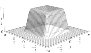
As an example let us fix d=2d=2 and α=β=110​(1,1)T\mathbf{\alpha}=\mathbf{\beta}=\tfrac{1}{10}(1,1)^{\mathrm{T}}. Figure 2 illustrates the two cases Bβ​(𝐉X​𝐱)B_{\mathbf{\beta}}(\mathbf{J}_{\text{X}}\mathbf{x}) and Bβ​(𝐉D​𝐱)B_{\mathbf{\beta}}(\mathbf{J}_{\text{D}}\mathbf{x}) in comparison to Bα​(𝐱)B_{\mathbf{\alpha}}(\mathbf{x}). For simplification and due to symmetry, both figures are restricted to the first quadrant, where the dashed line delimits the support of BαB_{\mathbf{\alpha}} or the shaded support of BβB_{\mathbf{\beta}} and the dotted line marks the inner plateau. The first case using 𝐉X\mathbf{J}_{\text{X}} is similar to the one-dimensional case, because β2=α2\beta_{2}=\alpha_{2} and 2​α1+β1=310≤122\alpha_{1}+\beta_{1}=\tfrac{3}{10}\leq\tfrac{1}{2}.

In the second case, cf. Figure 2 (b), we have for any point 𝐪\mathbf{q}, 0<q1<2​α10<q_{1}<2\alpha_{1}, 12<q2<12+α2−|α1−q1|\tfrac{1}{2}<q_{2}<\tfrac{1}{2}+\alpha_{2}-|\alpha_{1}-q_{1}| that Bα​(𝐪)≠0B_{\mathbf{\alpha}}(\mathbf{q})\neq 0 and Bβ​(𝐉D​𝐪)≠0B_{\mathbf{\beta}}(\mathbf{J}_{\text{D}}\mathbf{q})\neq 0. In order to fulfill MR2, cf. Lemma 2.5, these coefficients a^𝐡\hat{a}_{\mathbf{h}} are in this illustration — due to multiplication with 𝐌−T\mathbf{M}^{-\mathrm{T}} — given by sampling a 11-periodic function. For the point 𝐪+(0,1)T\mathbf{q}+(0,1)^{\mathrm{T}} we have by symmetry, Bα​(𝐪+(0,1)T)=Bα​(𝐩)≠0B_{\mathbf{\alpha}}(\mathbf{q}+(0,1)^{\mathrm{T}})=B_{\mathbf{\alpha}}(\mathbf{p})\neq 0 and Bβ​(𝐉D​(𝐪+(0,1)T)=Bβ​(𝐉D​𝐩)=0CLOSEB_{\mathbf{\beta}}(\mathbf{J}_{\text{D}}(\mathbf{q}+(0,1)^{\mathrm{T}})=B_{\mathbf{\beta}}(\mathbf{J}_{\text{D}}\mathbf{p})=0. This holds for any of the mentioned points 𝐪\mathbf{q} and yields a contradiction to MR2, if only the absolute value of the determinant of 𝐌\mathbf{M} is large enough, such that any point 𝐌−T​𝐤\mathbf{M}^{-\mathrm{T}}\mathbf{k}, 𝐤∈𝒢​(𝐌T)\mathbf{k}\in\mathcal{G}_{\mathrm{}}(\mathbf{M}^{\mathrm{T}}), corresponds to one point 𝐪\mathbf{q}.

4 Scaling functions of de la Vallée Poussin type

This section is devoted to a construction of scaling functions and in the dyadic case their wavelets having an arbitrary smooth decay in their Fourier coefficients.

Definition 4.1.

We call a function g:ℝd→ℝg:\mathbb{R}^{d}\to\mathbb{R} admissible if the following two properties are fulfilled

  1. F1)

    g⁡(𝐱)≥0g(\mathbf{x})\geq 0, for all 𝐱∈supp⁡g⊂ℝd\mathbf{x}\in\operatorname{supp}g\subset\mathbb{R}^{d}, and g⁡(𝐱)>0g(\mathbf{x})>0, 𝐱∈𝒬d\mathbf{x}\in\mathcal{Q}_{d},

  2. F2)

    ∑𝐳∈ℤdg⁡(𝐱+𝐳)=1\sum\limits_{\mathbf{z}\in\mathbb{Z}^{d}}g(\mathbf{x}+\mathbf{z})=1, for all 𝐱∈ℝd\mathbf{x}\in\mathbb{R}^{d}.

A special class of admissible functions are the centered box splines MΞcM_{\Xi}^{c}, cf. [5, Chapter I], where the dd-dimensional unit matrix 𝐄d\mathbf{E}_{d} is a subset of the vectors in Ξ\Xi. The function BαB_{\mathbf{\alpha}} from (12) is a special case of the centered box splines, more precisely with Ξ=(𝐞1,…,𝐞d,α1​𝐞1,…,αd​𝐞d)\Xi=\bigl(\mathbf{e}_{1},\ldots,\mathbf{e}_{d},\alpha_{1}\mathbf{e}_{1},\ldots,\alpha_{d}\mathbf{e}_{d}\bigr), where 𝐞j\mathbf{e}_{j} denotes the jjth unit vector. Of course, an admissible function gg can also be chosen, such that it is arbitrarily smooth, e.g. by adding the last dd vectors multiple times to the matrix Ξ\Xi. Introducing the possibility to choose a smooth function gg follows the idea, that sampling a smooth function to obtain the Fourier coefficients yields a certain localization, which was used in the one-dimensional case for example in [12].

For a regular matrix 𝐉∈ℤd×d\mathbf{J}\in\mathbb{Z}^{d\times d}, a function f:ℝd→ℂf:\mathbb{R}^{d}\to\mathbb{C} is called summable with respect to 𝐉\mathbf{J}, if for all 𝐱∈ℝd\mathbf{x}\in\mathbb{R}^{d}

f𝐉​(𝐱):=∑𝐳∈ℤdf⁡(𝐱+𝐉T​𝐳)<∞​.f^{\mathbf{J}}(\mathbf{x}):=\sum_{\mathbf{z}\in\mathbb{Z}^{d}}f(\mathbf{x}+\mathbf{J}^{\mathrm{T}}\mathbf{z})<\infty\text{.}

Any admissible function gg is summable with respect to 𝐉\mathbf{J}.

For any two functions f1,f2:ℝd→ℂf_{1},f_{2}:\mathbb{R}^{d}\to\mathbb{C} and a regular matrix 𝐉∈ℤd×d\mathbf{J}\in\mathbb{Z}^{d\times d}, where f1f_{1} is summable with respect to 𝐉\mathbf{J}, we define the operator

Φ𝐉(f1,f2):=f1𝐉(∘)f2(𝐉−T∘)=(∑𝐳∈ℤdf1(∘−𝐉T𝐳))f2(𝐉−T∘)\Phi_{\mathbf{J}}\mathopen{(}f_{1},f_{2}\mathclose{)}:=f_{1}^{\mathbf{J}}(\circ)f_{2}(\mathbf{J}^{-\mathrm{T}}\circ)=\Biggr(\sum_{\mathbf{z}\in\mathbb{Z}^{d}}f_{1}(\circ-\mathbf{J}^{\mathrm{T}}\mathbf{z})\Biggr)f_{2}(\mathbf{J}^{-\mathrm{T}}\circ)

and for a vector of regular integral matrices 𝐉1,…,𝐉n∈ℤd×d\mathbf{J}_{1},\ldots,\mathbf{J}_{n}\in\mathbb{Z}^{d\times d}, n∈ℕn\in\mathbb{N}, we define the matrix vectors

𝒥l,k:={(𝐉j)j=lk∈(ℤd×d)k−l+1 if ​1≤l≤k≤n​,∅else,\mathcal{J}_{l,k}:=\begin{cases}\bigl(\mathbf{J}_{j}\bigr)_{j=l}^{k}\in\bigl(\mathbb{Z}^{d\times d}\bigr)^{k-l+1}&\mbox{ if }1\leq l\leq k\leq n\text{,}\\ \emptyset&\mbox{else,}\end{cases}

where we restrict the set of matrices by writing 𝒥l,k∈𝒳k−l+1\mathcal{J}_{l,k}\in\mathcal{X}^{k-l+1} for matrices 𝐉j\mathbf{J}_{j}, j=l,…,kj=l,\ldots,k from the set 𝒳\mathcal{X}. A matrix vector 𝒥l,k\mathcal{J}_{l,k} only consisting of matrices having |det𝐉j|=2|\det\mathbf{J}_{j}|=2, j=1,…,nj=1,\ldots,n, is called dyadic.

For a matrix vector 𝒥1,n\mathcal{J}_{1,n} the functions B𝒥l,kB_{\!\!\mathcal{J}_{l,k}}, k∈{1,…,n}k\in\{1,\ldots,n\} are recursively defined by

B𝒥l,k:={g if ​l≥k+1​,Φ𝐉l​(g,B𝒥l+1,k) if ​l=k,k−1,…,1​,B_{\!\!\mathcal{J}_{l,k}}:=\begin{cases}g&\mbox{ if }l\geq k+1\text{,}\\ \Phi_{\mathbf{J}_{l}}\mathopen{\big(}g,B_{\!\!\mathcal{J}_{l+1,k}}\mathclose{\big)}&\mbox{ if }l=k,k-1,\ldots,1\text{,}\end{cases}

where g:ℝd→ℂg:\mathbb{R}^{d}\to\mathbb{C} is an admissible function.

Definition 4.2.

Let 𝐌0∈ℤd×d\mathbf{M}_{0}\in\mathbb{Z}^{d\times d} be a regular matrix, m0=|det𝐌0|>0m_{0}=|\det\mathbf{M}_{0}|>0, and let 𝒥1,n∈(ℤd×d)n\mathcal{J}_{1,n}\in\bigl(\mathbb{Z}^{d\times d}\bigr)^{n}, n∈ℕn\in\mathbb{N}, be a vector of regular matrices 𝐉l\mathbf{J}_{l}, l=1,…,nl=1,\ldots,n. We further denote for each l=1,…,nl=1,\ldots,n, that 𝐌l:=𝐉l⋅…⋅𝐉1​𝐌0\mathbf{M}_{l}:=\mathbf{J}_{l}\cdot\ldots\cdot\mathbf{J}_{1}\mathbf{M}_{0} and ml:=|det𝐌l|m_{l}:=|\det\mathbf{M}_{l}|.

The functions φ𝐌l𝒥l+1,n\varphi_{\mathbf{M}_{l}}^{\mathcal{J}_{l+1,n}}, l=0,…,nl=0,\ldots,n, which are defined by their Fourier coefficients

c𝐤​(φ𝐌l𝒥l+1,n)\displaystyle c_{\mathbf{k}}\bigl(\varphi_{\mathbf{M}_{l}}^{\mathcal{J}_{l+1,n}}\bigr) :=1mlB𝒥l+1,n(𝐌l−T𝐤),𝐤∈ℤd×d,l=0,…,n,\displaystyle:=\frac{1}{\sqrt{m_{l}}}B_{\!\!\mathcal{J}_{l+1,n}}(\mathbf{M}_{l}^{-\mathrm{T}}\mathbf{k}),\quad\mathbf{k}\in\mathbb{Z}^{d\times d},\ l=0,\ldots,n\text{,}

are called scaling functions of de la Vallée Poussin type.

We further introduce the corresponding spaces, which we denote by

V𝐌l𝒥l+1,n:=span⁡{T𝐲​φ𝐌l𝒥l+1,n;𝐲∈𝒫​(𝐌l)},l∈{0,…,n}​.V_{\mathbf{M}_{l}}^{\mathcal{J}_{l+1,n}}:=\operatorname{span}\Bigl\{\text{T}_{\mathbf{y}}\varphi_{\mathbf{M}_{l}}^{\mathcal{J}_{l+1,n}}\ ;\ \mathbf{y}\in\mathcal{P}_{\!\mathrm{}}(\mathbf{M}_{l})\Bigr\},\quad l\in\{0,\ldots,n\}\text{.}

Let Cr​(𝕋d)C^{r}(\mathbb{T}^{d}), r∈ℕr\in\mathbb{N}, denote the space of functions f:𝕋d→ℂf:\mathbb{T}^{d}\to\mathbb{C} whose rrth directional derivatives are continuous.

Theorem 4.3.

Let the scaling functions of de la Vallée Poussin type φ𝐌l𝒥l+1,n\varphi_{\mathbf{M}_{l}}^{\mathcal{J}_{l+1,n}}, l=0,…,nl=0,\ldots,n, n∈ℕn\in\mathbb{N}, be given as in Definition 4.2. Then the following statements hold

  1. a)

    The spaces V𝐌l𝒥l+1,nV_{\mathbf{M}_{l}}^{\mathcal{J}_{l+1,n}} are nested, i.e.

    φ𝐌l𝒥l+1,n∈V𝐌l+1𝒥l+2,n holds for ​l=0,…,n−1​.\varphi_{\mathbf{M}_{l}}^{\mathcal{J}_{l+1,n}}\in V_{\mathbf{M}_{l+1}}^{\mathcal{J}_{l+2,n}}\quad\text{ holds for }l=0,\ldots,n-1\text{.}
  2. b)

    For each l∈{0,…,n}l\in\{0,\ldots,n\}, the shifts T𝐲​φ𝐌l𝒥l+1,n\text{T}_{\mathbf{y}}\varphi_{\mathbf{M}_{l}}^{\mathcal{J}_{l+1,n}}, 𝐲∈𝒫​(𝐌l)\mathbf{y}\in\mathcal{P}_{\!\mathrm{}}(\mathbf{M}_{l}), are linearly independent.

  3. c)

    Let g∈Cr​(ℝd),r∈ℕg\in C^{r}(\mathbb{R}^{d}),r\in\mathbb{N}. Then, for l∈{0,…,n}l\in\{0,\ldots,n\} it holds B𝒥l+1,n(𝐌l−T∘)∈Cr(ℝd).B_{\!\!\mathcal{J}_{l+1,n}}(\mathbf{M}_{l}^{-\mathrm{T}}\circ)\in C^{r}(\mathbb{R}^{d})\text{.}

Proof.
  1. a)

    Let l∈{0,…,n−1}l\in\{0,\ldots,n-1\} be given. We define

    a^l,𝐡:=|det𝐉l+1|​g𝐉l+1​(𝐌l−T​𝐡),𝐡∈𝒢​(𝐌l+1T)\hat{a}_{l,\mathbf{h}}:=\sqrt{|\det\mathbf{J}_{l+1}|}g^{\mathbf{J}_{l+1}}(\mathbf{M}_{l}^{-\mathrm{T}}\mathbf{h}),\quad\mathbf{h}\in\mathcal{G}_{\mathrm{}}(\mathbf{M}^{\mathrm{T}}_{l+1}) (13)

    and use the unique decomposition of any 𝐤∈ℤd\mathbf{k}\in\mathbb{Z}^{d} into 𝐤=𝐡+𝐌l+1T​𝐳\mathbf{k}=\mathbf{h}+\mathbf{M}_{l+1}^{\mathrm{T}}\mathbf{z}, 𝐡∈𝒢​(𝐌l+1T)\mathbf{h}\in\mathcal{G}_{\mathrm{}}(\mathbf{M}_{l+1}^{\mathrm{T}}), 𝐳∈ℤd\mathbf{z}\in\mathbb{Z}^{d}, to obtain

    c𝐡+𝐌l+1T​𝐳​(φ𝐌l𝒥l+1,n)=1mjB𝒥l+1,n(𝐌l−T(𝐡+𝐌l+1T𝐳))=1mj​Φ𝐉l+1​(g,B𝒥l+2,n)​(𝐌l−T​𝐡+𝐉l+1T​𝐳)=a^l,𝐡​1ml+1​B𝒥l+2,n​(𝐌l+1−T​𝐡+𝐳)=a^l,𝐡​c𝐡+𝐌l+1T​𝐳​(φ𝐌l+1𝒥l+2,n)​.\begin{split}c_{\mathbf{h}+\mathbf{M}_{l+1}^{\mathrm{T}}\mathbf{z}}\bigl(\varphi_{\mathbf{M}_{l}}^{\mathcal{J}_{l+1,n}}\bigr)&=\frac{1}{\sqrt{m_{j}}}B_{\!\!\mathcal{J}_{l+1,n}}\Bigl(\mathbf{M}_{l}^{-\mathrm{T}}\bigl(\mathbf{h}+\mathbf{M}_{l+1}^{\mathrm{T}}\mathbf{z}\bigl)\Bigl)\\ &=\frac{1}{\sqrt{m_{j}}}\Phi_{\mathbf{J}_{l+1}}\mathopen{(}g,B_{\!\!\mathcal{J}_{l+2,n}}\mathclose{)}\bigl(\mathbf{M}_{l}^{-\mathrm{T}}\mathbf{h}+\mathbf{J}_{l+1}^{\mathrm{T}}\mathbf{z}\bigr)\\ &=\hat{a}_{l,\mathbf{h}}\frac{1}{\sqrt{m_{l+1}}}B_{\!\!\mathcal{J}_{l+2,n}}\bigl(\mathbf{M}_{l+1}^{-\mathrm{T}}\mathbf{h}+\mathbf{z}\bigr)\\ &=\hat{a}_{l,\mathbf{h}}c_{\mathbf{h}+\mathbf{M}_{l+1}^{\mathrm{T}}\mathbf{z}}\bigl(\varphi_{\mathbf{M}_{l+1}}^{\mathcal{J}_{l+2,n}}\bigr)\text{.}\end{split}

    Hence the statement follows with (3).

  2. b)

    For 𝐡∈𝒢S​(𝐌lT)\mathbf{h}\in\mathcal{G}_{\mathrm{S}}(\mathbf{M}_{l}^{\mathrm{T}}) and l∈{0,…,n}l\in\{0,\ldots,n\} it holds c𝐡​(φ𝐌l𝒥l+1,n)=1ml​B𝒥l+1,n​(𝐌l−T​𝐡)c_{\mathbf{h}}(\varphi_{\mathbf{M}_{l}}^{\mathcal{J}_{l+1,n}})=\frac{1}{\sqrt{m_{l}}}B_{\!\!\mathcal{J}_{l+1,n}}(\mathbf{M}_{l}^{-\mathrm{T}}\mathbf{h}) and 𝐌l−T​𝐡∈𝒬d\mathbf{M}_{l}^{-\mathrm{T}}\mathbf{h}\in\mathcal{Q}_{d}. The linear independence of translates does not depend on the choice of the generating set 𝒢​(𝐌lT)\mathcal{G}_{\mathrm{}}(\mathbf{M}_{l}^{\mathrm{T}}). We will restrict the rest of the proof to the generating set 𝒢S​(𝐌lT)\mathcal{G}_{\mathrm{S}}(\mathbf{M}_{l}^{\mathrm{T}}).

    For l=nl=n we have for 𝐱∈𝒬d\mathbf{x}\in\mathcal{Q}_{d}, that B𝒥n+1,n​(𝐱)=g⁡(𝐱)>0B_{\!\!\mathcal{J}_{n+1,n}}(\mathbf{x})=g(\mathbf{x})>0 and hence c𝐡​(φ𝐌n𝒥n+1,n)≠0c_{\mathbf{h}}(\varphi_{\mathbf{M}_{n}}^{\mathcal{J}_{n+1,n}})\neq 0 for 𝐡∈𝒢S​(𝐌nT)\mathbf{h}\in\mathcal{G}_{\mathrm{S}}(\mathbf{M}_{n}^{\mathrm{T}}).

    For 0≤l<n0\leq l<n the statement follows by induction over ll. By induction hypothesis B𝒥l+2,n​(𝐱)>0B_{\!\!\mathcal{J}_{l+2,n}}(\mathbf{x})>0 for 𝐱∈𝒬d\mathbf{x}\in\mathcal{Q}_{d} and for each 𝐲∈ℝd\mathbf{y}\in\mathbb{R}^{d} there exist 𝐱′∈𝒬d,𝐳′∈ℤd\mathbf{x}^{\prime}\in\mathcal{Q}^{d},\mathbf{z}^{\prime}\in\mathbb{Z}^{d} such that 𝐲=𝐱′+𝐳\mathbf{y}=\mathbf{x}^{\prime}+\mathbf{z}. Hence if 𝐲=𝐉l+1−T​𝐱∉𝒬d\mathbf{y}=\mathbf{J}_{l+1}^{-\mathrm{T}}\mathbf{x}\notin\mathcal{Q}_{d}, we have 𝐱′∈𝒬d\mathbf{x}^{\prime}\in\mathcal{Q}_{d}. The shift by 𝐳\mathbf{z} does not affect the corresponding first factor because we have 𝐲′=𝐱−𝐉j+1T​𝐳\mathbf{y}^{\prime}=\mathbf{x}-\mathbf{J}_{j+1}^{\mathrm{T}}\mathbf{z}. We obtain

    B𝒥l+1,n​(𝐱)\displaystyle B_{\!\!\mathcal{J}_{l+1,n}}(\mathbf{x}) =Φ𝐉l+1​(g,B𝒥l+2,n)​(𝐱)\displaystyle=\Phi_{\mathbf{J}_{l+1}}\mathopen{(}g,B_{\!\!\mathcal{J}_{l+2,n}}\mathclose{)}(\mathbf{x})
    =(∑𝐳∈ℤg⁡(𝐱+𝐉l+1T​𝐳))​B𝒥l+2,n​(𝐉l+1−T​𝐲′)>0​,\displaystyle=\Biggl(\sum_{\mathbf{z}\in\mathbb{Z}}g(\mathbf{x}+\mathbf{J}^{\mathrm{T}}_{l+1}\mathbf{z})\Biggr)B_{\!\!\mathcal{J}_{l+2,n}}(\mathbf{J}_{l+1}^{-\mathrm{T}}\mathbf{y}^{\prime})>0\text{,}

    because gg is nonnegative. Hence c𝐡​(φ𝐌l𝒥l+1,n)≠0c_{\mathbf{h}}\bigl(\varphi_{\mathbf{M}_{l}}^{\mathcal{J}_{l+1,n}}\bigr)\neq 0 for all 𝐡∈𝒢S​(𝐌lT)\mathbf{h}\in\mathcal{G}_{\mathrm{S}}(\mathbf{M}_{l}^{\mathrm{T}}) and the translates T𝐲​φ𝐌l𝒥l+1,n\text{T}_{\mathbf{y}}\varphi_{\mathbf{M}_{l}}^{\mathcal{J}_{l+1,n}}, 𝐲∈𝒫S​(𝐌l)\mathbf{y}\in\mathcal{P}_{\!\mathrm{S}}(\mathbf{M}_{l}) are linearly independent by [10, Corollary 3.5].

  3. c)

    For l=nl=n the function B𝒥l+1,n(𝐌l−T∘)B_{\!\!\mathcal{J}_{l+1,n}}(\mathbf{M}_{l}^{-\mathrm{T}}\circ) is just a scaled, sheared and rotated version of the function gg and hence by assumption in Cr​(ℝd)C^{r}(\mathbb{R}^{d}). For 0≤l<n0\leq l<n we obtain the statement by applying the same induction as in b).∎

The coefficients a^l,𝐡\hat{a}_{l,\mathbf{h}}, l<nl<n, defined in the proof Theorem 4.3 a) can also be interpreted as sampling the function |det𝐉l+1|g𝐉l+1(𝐌l−T∘)\sqrt{|\det\mathbf{J}_{l+1}|}g^{\mathbf{J}_{l+1}}(\mathbf{M}_{l}^{-\mathrm{T}}\circ) at a subset of the integer vectors. As long as only these coefficients are needed, e.g. for the orthonormalization utilizing Lemma 2.2, they can easily be obtained using the summation with respect to 𝐉l+1T\mathbf{J}^{\mathrm{T}}_{l+1} of the function gg, which is analogously to Theorem 4.3 c) a function in Cr​(ℝ)C^{r}(\mathbb{R}).

Lemma 4.4.

For n∈ℕn\in\mathbb{N}, 𝒥1,n∈{𝐉X,𝐉Y,𝐉D}n\mathcal{J}_{1,n}\in\{\mathbf{J}_{X},\mathbf{J}_{Y},\mathbf{J}_{D}\}^{n}, and g=M𝐄dc=χ[−12,12]dg=M_{\mathbf{E}_{d}}^{c}=\mathbf{\chi}_{[-\frac{1}{2},\frac{1}{2}]^{d}}, the characteristic function of [−12,12]d[-\tfrac{1}{2},\tfrac{1}{2}]^{d}, the scaling functions of de la Vallée Poussin type φ𝐌l𝒥l+1,n\varphi_{\mathbf{M}_{l}}^{\mathcal{J}_{l+1,n}}, l=0,…,nl=0,\ldots,n, yield the Dirichlet kernels D𝐌lreD_{\mathbf{M}_{l}}^{\text{re}} from [10, Section 6].

Proof.

For l=nl=n this is evident. For l=n−1,n−2,…,0l=n-1,\,n-2,\ldots,0 we again apply induction over ll and the fact, that the sum in

B𝒥l+1,n=(∑𝐳∈ℤdχ𝒬d(∘−𝐉l+1T𝐳))B𝒥l+2,n(𝐉l+1−T∘)B_{\!\!\mathcal{J}_{l+1,n}}=\Biggl(\sum_{\mathbf{z}\in\mathbb{Z}^{d}}\mathbf{\chi}_{\mathcal{Q}_{d}}(\circ-\mathbf{J}_{l+1}^{\mathrm{T}}\mathbf{z})\Biggr)B_{\!\!\mathcal{J}_{l+2,n}}(\mathbf{J}_{l+1}^{-\mathrm{T}}\circ)

consists only of one point or a certain number of points of χ[−12,12]d\mathbf{\chi}_{[-\frac{1}{2},\frac{1}{2}]^{d}} at the boundary. The multiplication following the summation yields B𝒥l+1,n=χ[−12,12]dB_{\!\!\mathcal{J}_{l+1,n}}=\mathbf{\chi}_{[-\frac{1}{2},\frac{1}{2}]^{d}}, l=0,…,nl=0,\ldots,n. ∎

In case of a dyadic vector 𝒥1,n\mathcal{J}_{1,n}, it is also possible to derive the corresponding wavelets. If we fix l∈{1,…,n}l\in\{1,\ldots,n\}, we obtain, that the elements 𝐯l∈𝒫​(𝐉lT)\{𝟎}\mathbf{v}_{l}\in\mathcal{P}_{\!\mathrm{}}(\mathbf{J}_{l}^{\mathrm{T}})\backslash\{\mathbf{0}\} and 𝐰l∈𝒫​(𝐉l)\{𝟎}\mathbf{w}_{l}\in\mathcal{P}_{\!\mathrm{}}(\mathbf{J}_{l})\backslash\{\mathbf{0}\} are uniquely determined due to |det𝐉l|=2|\det\mathbf{J}_{l}|=2. The function B~𝒥l,k\tilde{B}_{\!\!\mathcal{J}_{l,k}}, 1≤l<k<n∈ℕ1\leq l<k<n\in\mathbb{N} is similarly to B𝒥l,kB_{\!\!\mathcal{J}_{l,k}} given by

B~𝒥l,k:=exp(−2πi∘T𝐰l)Φ𝐉l(T̂𝐯lg,B𝒥l+1,k),\tilde{B}_{\mathcal{J}_{l,k}}:=\exp(-2\pi\mathrm{i}\circ^{\mathrm{T}}\mathbf{w}_{l})\,\Phi_{\mathbf{J}_{l}}\mathopen{\Big(}\text{\^{T}}_{\mathbf{v}_{l}}g,B_{\mathcal{J}_{l+1,k}}\mathclose{\Big)}\text{,}

where T̂𝐯g:=g(∘−𝐯)\text{\^{T}}_{\mathbf{v}}g:=g(\circ-\mathbf{v}). It differs from B𝒥l,kB_{\!\!\mathcal{J}_{l,k}} just in the first step of the recursive definition, where instead of gg, the shifted function T̂𝐯l​g\text{\^{T}}_{\mathbf{v}_{l}}g is used and a modulation is introduced by the factor e−2πi∘T𝐰l\mathrm{e}^{-2\pi\mathrm{i}\circ^{\mathrm{T}}\mathbf{w}_{l}}.

Definition 4.5.

Let the matrix 𝐌0∈ℤd×d\mathbf{M}_{0}\in\mathbb{Z}^{d\times d} be regular, m0=|det𝐌0|>0m_{0}=|\det\mathbf{M}_{0}|>0, a dyadic vector 𝒥1,n\mathcal{J}_{1,n}, n∈ℕn\in\mathbb{N}, of matrices be given and denote 𝐌l\mathbf{M}_{l}, l=1,…,nl=1,\ldots,n, as in Definition 4.2.

The functions ψ𝐌l𝒥l+1,n\psi_{\mathbf{M}_{l}}^{\mathcal{J}_{l+1,n}}, which are defined by their Fourier coefficients as

c𝐤​(ψ𝐌l𝒥l+1,n)\displaystyle c_{\mathbf{k}}\bigl(\psi_{\mathbf{M}_{l}}^{\mathcal{J}_{l+1,n}}\bigr) =1mlB~𝒥l+1,n(𝐌l−T𝐤),𝐤∈ℤd×d,l=0,…,n−1,\displaystyle=\frac{1}{\sqrt{m_{l}}}\tilde{B}_{\!\!\mathcal{J}_{l+1,n}}(\mathbf{M}_{l}^{-\mathrm{T}}\mathbf{k}),\quad\mathbf{k}\in\mathbb{Z}^{d\times d},\quad l=0,\ldots,n-1\text{,}

are called wavelets of de la Vallée Poussin type.

We introduce the corresponding spaces of their shifts for l∈{0,…,n−1}l\in\{0,\ldots,n-1\} as

W𝐌l𝒥l+1,n:=span⁡{T𝐲​ψ𝐌l𝒥l+1,n;𝐲∈𝒫​(𝐌l)}​.W_{\mathbf{M}_{l}}^{\mathcal{J}_{l+1,n}}:=\operatorname{span}\Bigl\{\text{T}_{\mathbf{y}}\psi_{\mathbf{M}_{l}}^{\mathcal{J}_{l+1,n}}\ ;\ \mathbf{y}\in\mathcal{P}_{\!\mathrm{}}(\mathbf{M}_{l})\Bigr\}\text{.}
Theorem 4.6.

For n∈ℕn\in\mathbb{N}, a regular matrix 𝐌0∈ℤd×d\mathbf{M}_{0}\in\mathbb{Z}^{d\times d} and a dyadic vector 𝒥1,n∈(ℤd×d)n\mathcal{J}_{1,n}\in\bigl(\mathbb{Z}^{d\times d}\bigr)^{n} of regular matrices, let the scaling functions of de la Vallée Poussin type φ𝐌l𝒥l+1,n\varphi_{\mathbf{M}_{l}}^{\mathcal{J}_{l+1,n}}, l=0,…,nl=0,\ldots,n, and the corresponding wavelets of de la Vallée Poussin type ψ𝐌l𝒥l+1,n\psi_{\mathbf{M}_{l}}^{\mathcal{J}_{l+1,n}}, l=0,…,n−1l=0,\ldots,n-1, be given.

Then, for each l∈{0,…,n−1}l\in\{0,\ldots,n-1\} the following holds.

  1. a)

    ψ𝐌l𝒥l+1,n∈V𝐌l+1𝒥l+2,n​.\psi_{\mathbf{M}_{l}}^{\mathcal{J}_{l+1,n}}\in V_{\mathbf{M}_{l+1}}^{\mathcal{J}_{l+2,n}}\text{.}

  2. b)

    V𝐌l+1𝒥l+2,n=V𝐌l𝒥l+1,n⊕W𝐌l𝒥l+1,n​.V_{\mathbf{M}_{l+1}}^{\mathcal{J}_{l+2,n}}=V_{\mathbf{M}_{l}}^{\mathcal{J}_{l+1,n}}\oplus W_{\mathbf{M}_{l}}^{\mathcal{J}_{l+1,n}}\text{.}

  3. c)

    The shifts T𝐲​ψ𝐌l𝒥l+1,n​,​𝐲∈𝒫​(𝐌l)​,\text{T}_{\mathbf{y}}\psi_{\mathbf{M}_{l}}^{\mathcal{J}_{l+1,n}}\text{,}\ \mathbf{y}\in\mathcal{P}_{\!\mathrm{}}(\mathbf{M}_{l})\text{,} are linearly independent.

  4. d)

    For g∈Cr​(ℝd),r∈ℕg\in C^{r}(\mathbb{R}^{d}),r\in\mathbb{N}, we have B~𝒥l+1,n(𝐌l−T∘)∈Cr(ℝd)\tilde{B}_{\mathcal{J}_{l+1,n}}(\mathbf{M}_{l}^{-\mathrm{T}}\circ)\in C^{r}(\mathbb{R}^{d}).

Proof.
  1. a)

    Analogously to the coefficients a^𝐡\hat{a}_{\mathbf{h}} from the proof of Theorem 4.3 a) we define for 𝐡∈𝒢​(𝐌l+1T)\mathbf{h}\in\mathcal{G}_{\mathrm{}}(\mathbf{M}_{l+1}^{\mathrm{T}}) the coefficients

    b^𝐡:=|det𝐉l+1|​exp⁡(−2​π​i​𝐤T​𝐌l−1​𝐰l+1)​(T̂𝐯l+1​g)𝐉l+1​(𝐌l−T​𝐡)=2​exp⁡(−2​π​i​𝐡T​𝐌l−1​𝐰l+1)​(∑𝐳∈ℤdg⁡(𝐌l−T​𝐡+𝐉l+1−T​𝐳−𝐯l+1))​.\begin{split}\hat{b}_{\mathbf{h}}:&=\sqrt{|\det\mathbf{J}_{l+1}|}\exp(-2\pi\mathrm{i}\mathbf{k}^{\mathrm{T}}\mathbf{M}_{l}^{-1}\mathbf{w}_{l+1})\bigl(\text{\^{T}}_{\mathbf{v}_{l+1}}g\bigr)^{\mathbf{J}_{l+1}}(\mathbf{M}^{-\mathrm{T}}_{l}\mathbf{h})\\ &=\sqrt{2}\exp(-2\pi\mathrm{i}\mathbf{h}^{\mathrm{T}}\mathbf{M}_{l}^{-1}\mathbf{w}_{l+1})\Bigl(\sum_{\mathbf{z}\in\mathbb{Z}^{d}}g(\mathbf{M}_{l}^{-\mathrm{T}}\mathbf{h}+\mathbf{J}_{l+1}^{-\mathrm{T}}\mathbf{z}-\mathbf{v}_{l+1})\Bigr)\text{.}\end{split} (14)

    The statement a) follows using the same steps as in the proof of Theorem 4.3 a), replacing B𝒥l+1,nB_{\mathcal{J}_{l+1,n}} by B~𝒥l+1,n\tilde{B}_{\mathcal{J}_{l+1,n}} and hence obtaining b^𝐡\hat{b}_{\mathbf{h}} instead of a^𝐡\hat{a}_{\mathbf{h}} in the calculations.

  2. b)

    The coefficients a^𝐡\hat{a}_{\mathbf{h}}, 𝐡∈𝒢​(𝐌l+1T)\mathbf{h}\in\mathcal{G}_{\mathrm{}}(\mathbf{M}_{l+1}^{\mathrm{T}}), from Theorem 4.3 a) and b^𝐡\hat{b}_{\mathbf{h}}, 𝐡∈𝒢​(𝐌l+1T)\mathbf{h}\in\mathcal{G}_{\mathrm{}}(\mathbf{M}_{l+1}^{\mathrm{T}}), from a) fulfill the requirements of Lemma 4.3 in [10], more precisely the values

    σ𝐡:=exp⁡(−2​π​i​𝐡T​𝐌l−1​𝐰l+1),𝐡∈𝒢​(𝐌l+1T)​,\sigma_{\mathbf{h}}:=\exp(-2\pi\mathrm{i}\mathbf{h}^{\mathrm{T}}\mathbf{M}_{l}^{-1}\mathbf{w}_{l+1}),\quad\mathbf{h}\in\mathcal{G}_{\mathrm{}}(\mathbf{M}_{l+1}^{\mathrm{T}})\text{,}

    even fulfill the requirements of Lemma 2.2, i.e. if the scaling functions of de la Vallée Poussin type φ𝐌l𝒥l+1,n\varphi_{\mathbf{M}_{l}}^{\mathcal{J}_{l+1,n}} and φ𝐌l+1𝒥l+2,n\varphi_{\mathbf{M}_{l+1}}^{\mathcal{J}_{l+2,n}} have orthonormal shifts, thus does the wavelet ψ𝐌l𝒥l+1,n\psi_{\mathbf{M}_{l}}^{\mathcal{J}_{l+1,n}}.

  3. c)

    The statement follows directly from b) and the linear independence of the shifts T𝐱​φ𝐌l𝒥l+1,n\text{T}_{\mathbf{x}}\varphi_{\mathbf{M}_{l}}^{\mathcal{J}_{l+1,n}}, 𝐱∈𝒫​(𝐌l)\mathbf{x}\in\mathcal{P}_{\!\mathrm{}}(\mathbf{M}_{l}), and T𝐲​φ𝐌l+1𝒥l+2,n\text{T}_{\mathbf{y}}\varphi_{\mathbf{M}_{l+1}}^{\mathcal{J}_{l+2,n}}, 𝐲∈𝒫​(𝐌l+1)\mathbf{y}\in\mathcal{P}_{\!\mathrm{}}(\mathbf{M}_{l+1}), cf. Theorem 4.3 b).

  4. d)

    Using the same modifications as in a), B~𝒥l+1,n(𝐌l−T∘)∈Cr(ℝd)\tilde{B}_{\mathcal{J}_{l+1,n}}(\mathbf{M}_{l}^{-\mathrm{T}}\circ)\in C^{r}(\mathbb{R}^{d}) holds analogously to Theorem 4.3 c).∎

Corollary 4.7.

For n∈ℕn\in\mathbb{N}, 𝒥1,n∈{𝐉X,𝐉Y,𝐉D}n\mathcal{J}_{1,n}\in\{\mathbf{J}_{X},\mathbf{J}_{Y},\mathbf{J}_{D}\}^{n} and g=M𝐄dcg=M_{\mathbf{E}_{d}}^{c} we obtain the Dirichlet wavelets ψ𝐍\psi_{\mathbf{N}} from [10, Eq. (42)] analogously to Lemma 4.4.

The presented construction of the scaling functions φ𝐌l𝒥l+1,n\varphi_{\mathbf{M}_{l}}^{\mathcal{J}_{l+1,n}} and wavelets ψ𝐌l𝒥l+1,n\psi_{\mathbf{M}_{l}}^{\mathcal{J}_{l+1,n}} of de la Vallée Poussin type introduces a huge variety of periodic anisotropic MRAs: On the one hand the function gg can be chosen with very less restrictions, especially it can be chosen arbitrarily smooth. Hence the scaling functions and wavelets are obtained by sampling an arbitrarily smooth function, e.g. by choosing box splines. The directional smoothness of gg does construct a certain directional smoothness with respect to the parallelotope defined by 𝐌lT​𝒬d\mathbf{M}_{l}^{\mathrm{T}}\mathcal{Q}_{d} on each level. On the other hand, the construction introduces the possibility to choose any matrix 𝐉l\mathbf{J}_{l} in the vector of scaling matrices. This extends the known Dirichlet case especially to the shear matrices, e.g. 𝐉𝐘+:=(1102)\mathbf{J}_{\mathbf{Y}}^{+}:=\bigl(\begin{smallmatrix}1&1\\ 0&2\end{smallmatrix}\bigr), but also any other integral regular matrix can be chosen. In the construction of the dyadic wavelets spanning the orthogonal complement, all matrices of determinant |det𝐉l|=2|\det{\mathbf{J}_{l}}|=2 are possible.

Taking a closer look at the coefficients a^l,𝐡\hat{a}_{l,\mathbf{h}} and b^l,𝐡\hat{b}_{l,\mathbf{h}}, that describe the two-scale relation for one level of the scaling function and the wavelet respectively, we see from (13) and (14), that both are obtained by sampling a certain sum of shifts of gg. If gg has finite support, these sums also have finite support. Moreover, these coefficients are obtained by sampling a function as smooth as gg.

A small extension to this construction, that was omitted in order to keep the notation simple, is the possibility to also chose gg for each level of the nested spaces separately, i.e. to introduce admissible functions g0,…,gng_{0},\ldots,g_{n} to define the sum in each level. Then of course the functions B𝒥l,k,B~𝒥l,kB_{\mathcal{J}_{l,k}},\tilde{B}_{\mathcal{J}_{l,k}} have to be adapted, to use glg_{l} in the operator Φ𝐉l​(gl,B𝒥l+1,n)\Phi_{\mathbf{J}_{l}}\mathopen{(}g_{l},B_{\!\!\mathcal{J}_{l+1,n}}\mathclose{)}. The coefficients a^l,𝐡\hat{a}_{l,\mathbf{h}} and b^l,𝐡\hat{b}_{l,\mathbf{h}} would each depend on glg_{l} and 𝐉l\mathbf{J}_{l}.

(a) supp⁡c𝐤​(φ𝐍(𝐉))\operatorname{supp}c_{\mathbf{k}}\bigl(\varphi_{\mathbf{N}}^{(\mathbf{J})}\bigr) and supp⁡c𝐤​(φ𝐌∅)\operatorname{supp}c_{\mathbf{k}}\bigl(\varphi_{\mathbf{M}}^{\emptyset}\bigr)
(b) supp⁡c𝐤​(ψ𝐍(𝐉))\operatorname{supp}c_{\mathbf{k}}\bigl(\psi_{\mathbf{N}}^{(\mathbf{J})}\bigr)
Refer to caption
(c) φ𝐌∅\varphi_{\mathbf{M}}^{\emptyset}
Refer to caption
(d) φ𝐍(𝐉)\varphi_{\mathbf{N}}^{(\mathbf{J})}
Refer to caption
(e) ψ𝐍(𝐉)\psi_{\mathbf{N}}^{(\mathbf{J})}
Refer to caption
(f) ψ𝐍(𝐉)\psi_{\mathbf{N}}^{(\mathbf{J})}, for α=𝟎\mathbf{\alpha}=\mathbf{0}
Figure 3: The support of the Fourier coefficients supp⁡c𝐤​(φ𝐍(𝐉))\operatorname{supp}c_{\mathbf{k}}\bigl(\varphi_{\mathbf{N}}^{(\mathbf{J})}\bigr), supp⁡c𝐤​(φ𝐌∅)\operatorname{supp}c_{\mathbf{k}}\bigl(\varphi_{\mathbf{M}}^{\emptyset}\bigr) and supp⁡c𝐤​(ψ𝐍(𝐉))\operatorname{supp}c_{\mathbf{k}}\bigl(\psi_{\mathbf{N}}^{(\mathbf{J})}\bigr) from Example 4.8 shown in 3 (a) and 3 (b). The corresponding functions φ𝐌∅\varphi_{\mathbf{M}}^{\emptyset}, φ𝐍(𝐉)\varphi_{\mathbf{N}}^{(\mathbf{J})} and ψ𝐍(𝐉)\psi_{\mathbf{N}}^{(\mathbf{J})} are plotted in 3 (c)-3 (e), where finally 3 (f) is constructed setting α=𝟎\mathbf{\alpha}=\mathbf{0} and hence obtaining a wavelet of Dirichlet type, to which ψ𝐍(𝐉)\psi_{\mathbf{N}}^{(\mathbf{J})} in 3 (e) looks more localized.
Example 4.8.

We look at the decomposition 𝐌:=(160128)=𝐉𝐍:=(1102)​(10−464)\mathbf{M}:=\bigl(\begin{smallmatrix}16&0\\ 12&8\end{smallmatrix}\bigr)=\mathbf{J}\mathbf{N}:=\bigl(\begin{smallmatrix}1&1\\ 0&2\end{smallmatrix}\bigr)\bigl(\begin{smallmatrix}10&-4\\ 6&4\end{smallmatrix}\bigr) and use the function g=Bαg=B_{\mathbf{\alpha}}, α=110​(1,1)T\mathbf{\alpha}=\tfrac{1}{10}(1,1)^{\mathrm{T}}, and n=1n=1. Then, we obtain a sequence of two functions, which consists of φ𝐌𝒥2,1=φ𝐌∅\varphi_{\mathbf{M}}^{\mathcal{J}_{2,1}}=\varphi_{\mathbf{M}}^{\emptyset} and φ𝐍𝒥1,1=φ𝐍(𝐉)\varphi_{\mathbf{N}}^{\mathcal{J}_{1,1}}=\varphi_{\mathbf{N}}^{(\mathbf{J})}. Both are given by their Fourier coefficients, cf. Definition 4.2. In Figure 3 (a), the support of both functions g(𝐌−T∘)g(\mathbf{M}^{-\mathrm{T}}\circ) in gray lines and Φ𝐉(g,g)(𝐍−T∘)\Phi_{\mathbf{J}}\mathopen{\big(}g,g\mathclose{\big)}(\mathbf{N}^{-\mathrm{T}}\circ) in black lines with gray shade is shown. For both, the dashed line marks the boundary of the support, while the dotted line encircles the area, where the function and hence the coefficients are constantly 1|det𝐍|=18\tfrac{1}{|\sqrt{\det\mathbf{N}}|}=\tfrac{1}{8}. The solid line further marks the boundary of the generating set, hence all integer points inside this parallelepiped including the left and lower boundary belong to the generating set 𝒢S​(𝐌T)\mathcal{G}_{\mathrm{S}}(\mathbf{M}^{\mathrm{T}}). One tenth along that line from any edge, the coefficients equal 12\tfrac{1}{2}. The maximum value c𝐤​(φ𝐍(𝐉))c_{\mathbf{k}}\bigl(\varphi_{\mathbf{N}}^{(\mathbf{J})}\bigr) on the additional nonzero area outside the parallelepiped is 14\tfrac{1}{4} on the solid gray line. Figure 3 (b) denotes the support of the corresponding wavelet, restricted to the gray area. Again, both dotted lines mark the plateaus in absolute values of the coefficients.

The corresponding functions φ𝐌∅\varphi_{\mathbf{M}}^{\emptyset}, φ𝐍(𝐉)\varphi_{\mathbf{N}}^{(\mathbf{J})} and ψ𝐍(𝐉)\psi_{\mathbf{N}}^{(\mathbf{J})} are shown in Figures 3 (c)-3 (e). In comparison to the wavelet of de la Vallée Poussin type in Figure 3 (e), a wavelet constructed by using g=χ𝒬dg=\chi_{\mathcal{Q}_{d}} is shown in Figure 3 (f). This corresponds to a wavelet of Dirichlet type, cf. Lemma 4.4, though for the original construction the shear matrix used in this example is not possible. The wavelet of de la Vallée Poussin type is better localized, which can be seen by the flatness of the function away from the origin. This is due to the continuity of the function gg, that is continuous for the de la Vallée Poussin type while being a characteristic function of the symmetric unit cube for the Dirichlet case.

5 A multiresolution analysis of de la Vallée Poussin type

While the construction from Section 4 introduces a huge variety of possibilities to choose gg and the scaling matrices 𝐉l\mathbf{J}_{l}, l=0,…,nl=0,\ldots,n, it introduces the necessity, that a scaling function φ𝐌l𝒥l+1,n\varphi_{\mathbf{M}_{l}}^{\mathcal{J}_{l+1,n}} or wavelet ψ𝐌l𝒥l+1,n\psi_{\mathbf{M}_{l}}^{\mathcal{J}_{l+1,n}} of de la Vallée Poussin type depends on all scaling matrices 𝐉l\mathbf{J}_{l}, the first ones 𝐉1,…,𝐉l\mathbf{J}_{1},\ldots,\mathbf{J}_{l} in a natural way, because they define 𝐌l\mathbf{M}_{l}, but also all following ones, i.e. 𝐉l+1,…,𝐉n\mathbf{J}_{l+1},\ldots,\mathbf{J}_{n}. This section will introduce a third condition of gg in order to reduce this dependency as far as possible.

For the one-dimensional case from Section 3, choosing the same function gg is equivalent to setting α=β\alpha=\beta. Theorem 4.1.3 in [18] yields, that these functions constitute an MRA if and only if α≤16\alpha\leq\tfrac{1}{6}. If α>16\alpha>\tfrac{1}{6}, Section 4 does still introduce a construction, though the Fourier coefficients are then constructed from three separated intervals, the support of (∑z∈ℤg(∘+2z))g(2−1∘)\bigr(\sum_{z\in\mathbb{Z}}g(\circ+2z)\bigl)g(2^{-1}\circ) consists of. Though, the first case is preferable due to it’s easier form and single interval of support.

For the multivariate case, we have at least to use φ𝐌l(𝐉l+1)\varphi_{\mathbf{M}_{l}}^{(\mathbf{J}_{l+1})}, for l<nl<n, because the first summation is g𝐉l+1g^{\mathbf{J}_{l}+1} and the matrices 𝐉l\mathbf{J}_{l} may vary even in the dyadic case from one ll to another which does not happen in the one-dimensional case for the factor 22. In the following, we examine the function gg further and introduce a description of its support, in order to characterize, for which cases the matrix 𝐉l+2\mathbf{J}_{l+2} does not affect φ𝐌l𝒥l+1,n\varphi_{\mathbf{M}_{l}}^{\mathcal{J}_{l+1,n}}, which hence simplifies to φ𝐌l(𝐉l+1)\varphi_{\mathbf{M}_{l}}^{(\mathbf{J}_{l+1})}. In order to do that, we look at three successive functions B𝒥k,nB_{\!\!\mathcal{J}_{k,n}}, k=l,l+1,l+2k=l,l+1,l+2, especially at their support. For simplification, we will first look at the case d=n=2d=n=2, where 𝒥1,2∈{𝐉X,𝐉Y,𝐉D}2\mathcal{J}_{1,2}\in\{\mathbf{J}_{\text{X}},\mathbf{J}_{\text{Y}},\mathbf{J}_{\text{D}}\}^{2} and discuss the general cases afterwards.

For 𝐩∈(−12,12)d\mathbf{p}\in\bigl(-\tfrac{1}{2},\frac{1}{2}\bigr)^{d} we define the domain Ω𝐩d\Omega_{\mathbf{p}}^{d} by

Ω𝐩d:=‘j=1d[−12−pj,12+pj]\Omega_{\mathbf{p}}^{d}:=\bigtimes_{j=1}^{d}\Bigl[-\frac{1}{2}-p_{j},\frac{1}{2}+p_{j}\Bigl]

and use the short cut Ωpd:=Ωp​𝟏d\Omega_{p}^{d}:=\Omega_{p\mathbf{1}}^{d} for p∈(−12,12)p\in\bigl(-\frac{1}{2},\frac{1}{2}\bigr). Immediately it follows

Lemma 5.1.

For any admissible function gg with supp⁡g⊆Ω𝐩d\operatorname{supp}g\subseteq\Omega_{\mathbf{p}}^{d}, 𝐩∈[0,12)d\mathbf{p}\in\bigl[0,\tfrac{1}{2}\bigr)^{d} it holds g⁡(𝐱)=1g(\mathbf{x})=1 for all 𝐱∈Ω−𝐩d\mathbf{x}\in\Omega_{-\mathbf{p}}^{d}.

Figure 4: Supports of three successive functions B𝒥j,2B_{\mathcal{J}_{j,2}}, j=1,2,3j=1,2,3, where 𝒥1,2=(𝐉D,𝐉D)\mathcal{J}_{1,2}=(\mathbf{J}_{\text{D}},\mathbf{J}_{\text{D}}) and supp⁡g∈Ω1202\operatorname{supp}g\in\Omega_{\frac{1}{20}}^{2}.

A typical situation is depicted in Figure 4, where we look at the support of three successive functions in the construction of nested spaces of de la Vallée Poussin type. To obtain independence from the initial matrix 𝐌0\mathbf{M}_{0} we take the first of the functions B𝒥j,nB_{\!\!\mathcal{J}_{j,n}} unscaled and apply the matrices 𝐉l,l=k+1,…,n\mathbf{J}_{l},l=k+1,\ldots,n to the argument of the function B𝒥j+1,nB_{\!\!\mathcal{J}_{j+1,n}}. We obtain a picture where the effect of summation, i.e. g(𝐉l)g^{(\mathbf{J}_{l})} compared to gg itself, is visible for example in the two hatched regions. Here both “inner” functions inherit a support by applying the summation, that only depends on the next upper support. If the support is bigger, than at some point the most inner function would also inherit a certain support that the second inner function obtained from the outer most one by summation. Due to symmetry we restrict the following illustrations again to the first quadrant.

For the rest of this section let gg have the two further properties, that

g(𝐱)=∏i=1dgi(xi), and suppgi⊂Ωpj1for i=1,…,d,g(\mathbf{x})=\prod_{i=1}^{d}g_{i}(x_{i}),\text{ and }\operatorname{supp}g_{i}\subset\Omega_{p_{j}}^{1}\quad\text{for }i=1,\ldots,d\text{,} (15)

where each gi:ℝ→ℝg_{i}:\mathbb{R}\to\mathbb{R}, i=1,…,di=1,\ldots,d, is itself a function having the properties F1) and F2) from Definition 4.1 for d=1d=1.

Then we need two auxiliary lemmata.

Lemma 5.2.

For 𝐉∈{𝐉X,𝐉Y}\mathbf{J}\in\{\mathbf{J}_{X},\mathbf{J}_{Y}\} and an admissible function g:ℝ2→ℂg:\mathbb{R}^{2}\to\mathbb{C} which also fulfills (15) and supp⁡g⊂Ωp2\operatorname{supp}g\subset\Omega_{p}^{2}, 0≤p≤160\leq p\leq\tfrac{1}{6}, it holds

Φ𝐉​(g,g)=g​.\Phi_{\mathbf{J}}\mathopen{(}g,g\mathclose{)}=g\text{.}
Proof.

The proof is given for 𝐉=𝐉X\mathbf{J}=\mathbf{J}_{X}, but can be obtained by the same arguments also for 𝐉=𝐉Y\mathbf{J}=\mathbf{J}_{Y}.

By assumptions, we have supp⁡g⊂Ωp2\operatorname{supp}g\subset\Omega_{p}^{2}, suppg(𝐉X−T∘)⊂𝐉XTΩp2\operatorname{supp}g(\mathbf{J}_{X}^{-\mathrm{T}}\circ)\subset\mathbf{J}_{X}^{\mathrm{T}}\Omega_{p}^{2}. For 𝐳=(0,z2)T∈ℤ2\mathbf{z}=(0,z_{2})^{\mathrm{T}}\in\mathbb{Z}^{2}, z1=0z_{1}=0, we have 𝐳+Ωp2∩𝐉X​Ωp2≠∅\mathbf{z}+\Omega_{p}^{2}\cap\mathbf{J}_{X}\Omega_{p}^{2}\neq\emptyset holds for 0≤p<120\leq p<\frac{1}{2} if and only if z2∈{−1,0,1}z_{2}\in\{-1,0,1\}. For z2∈{−1,0,1}z_{2}\in\{-1,0,1\}, the statements ∀z1∈ℤ\{0}:(𝐉XT​𝐳+Ωp2)∩𝐉X​Ωp2≠∅\forall z_{1}\in\mathbb{Z}\backslash\{0\}:(\mathbf{J}_{X}^{\mathrm{T}}\mathbf{z}+\Omega_{p}^{2})\cap\mathbf{J}_{X}\Omega_{p}^{2}\neq\emptyset and p≤16p\leq\tfrac{1}{6} are equivalent. Hence for 𝐱∈Ω(p,−p)T2⊂𝐉X​Ω(p,−p)T2\mathbf{x}\in\Omega_{(p,-p)^{\mathrm{T}}}^{2}\subset\mathbf{J}_{X}\Omega_{(p,-p)^{\mathrm{T}}}^{2} we obtain using property F2)

∑𝐳∈ℤ2g⁡(𝐱+𝐉XT​𝐳)=g⁡(𝐱)=g⁡(𝐉X−T​𝐱)=1​.\sum_{\mathbf{z}\in\mathbb{Z}^{2}}g(\mathbf{x}+\mathbf{J}_{X}^{\mathrm{T}}\mathbf{z})=g(\mathbf{x})=g(\mathbf{J}_{X}^{-\mathrm{T}}\mathbf{x})=1\text{.}

For 𝐱∈Ωp2\mathbf{x}\in\Omega_{p}^{2}, |x2|>12−p|x_{2}|>\tfrac{1}{2}-p, the sum over 𝐳∈ℤd\mathbf{z}\in\mathbb{Z}^{d} covers a second nonzero index despite 𝐳=𝟎\mathbf{z}=\mathbf{0}: z2=1z_{2}=1 for x2<−12+px_{2}<-\tfrac{1}{2}+p and z2=−1z_{2}=-1 for x2>12+px_{2}>\tfrac{1}{2}+p. Then, we have two cases: Due to |x1|<12−p|x_{1}|<\tfrac{1}{2}-p together with F2) of gg the sum is 11 and hence

(∑𝐳∈ℤ2g⁡(𝐱+𝐉XT​𝐳))​g​(𝐉X−T​𝐱)=g⁡(𝐉X−T​𝐱)=g⁡(𝐱)​.\Bigl(\sum_{\mathbf{z}\in\mathbb{Z}^{2}}g(\mathbf{x}+\mathbf{J}_{X}^{\mathrm{T}}\mathbf{z})\Bigr)g(\mathbf{J}_{X}^{-\mathrm{T}}\mathbf{x})=g(\mathbf{J}_{X}^{-\mathrm{T}}\mathbf{x})=g(\mathbf{x})\text{.}

Further, for 12−p≤|x1|≤12+p\tfrac{1}{2}-p\leq|x_{1}|\leq\tfrac{1}{2}+p, the summation does not simplify to 11 due to the dilation caused by 𝐉X−T\mathbf{J}_{X}^{-\mathrm{T}}. It holds

(∑𝐳∈ℤ2g⁡(𝐱+𝐉XT​𝐳))​g​(𝐉X−T​𝐱)\displaystyle\Bigl(\sum_{\mathbf{z}\in\mathbb{Z}^{2}}g(\mathbf{x}+\mathbf{J}_{X}^{\mathrm{T}}\mathbf{z})\Bigr)g(\mathbf{J}_{X}^{-\mathrm{T}}\mathbf{x}) =g1​(x1)​(g2​(x2)+g2​(x2±1))​g1​(x12)​g2​(x2)\displaystyle=g_{1}(x_{1})\Bigl(g_{2}(x_{2})+g_{2}(x_{2}\pm 1)\Bigr)g_{1}\Bigl(\frac{x_{1}}{2}\Bigr)g_{2}(x_{2})
=g1​(x1)​g2​(x2)=g⁡(𝐱)​.∎\displaystyle=g_{1}(x_{1})g_{2}(x_{2})=g(\mathbf{x})\text{.}\qed
Lemma 5.3.

For 0≤p≤160\leq p\leq\tfrac{1}{6} let a function g:ℝ2→ℝg:\mathbb{R}^{2}\to\mathbb{R} be given as in (15), having supp⁡g⊂Ωp2\operatorname{supp}g\subset\Omega_{p}^{2}. Then it holds for 𝐉∈{𝐉X,𝐉Y,𝐉D}\mathbf{J}\in\{\mathbf{J}_{X},\mathbf{J}_{Y},\mathbf{J}_{D}\}, that

Φ𝐉​(g,Φ𝐉D​(g,g))=Φ𝐉​(g,g)\Phi_{\mathbf{J}}\mathopen{\big(}g,\Phi_{\mathbf{J}_{D}}\mathopen{(}g,g\mathclose{)}\mathclose{\big)}=\Phi_{\mathbf{J}}\mathopen{(}g,g\mathclose{)} (16)

if and only if

(⋃𝐳∈ℤ2Ωp2+𝐉T​𝐳)∩𝐉T​Ωp2⊂𝐉T​𝐉DT​Ω−p2​.\Biggl(\bigcup_{\mathbf{z}\in\mathbb{Z}^{2}}\Omega_{p}^{2}+\mathbf{J}^{\mathrm{T}}\mathbf{z}\Biggr)\cap\mathbf{J}^{\mathrm{T}}\Omega_{p}^{2}\ \ \subset\ \ \mathbf{J}^{\mathrm{T}}\mathbf{J}_{D}^{\mathrm{T}}\Omega_{-p}^{2}\text{.} (17)
Proof.

Writing the operator on the left hand side of (16) we obtain

Φ𝐉(g,Φ𝐉D(g,g))=(∑𝐳∈ℤ2g(∘+𝐉T𝐳))(∑𝐲∈ℤ2g(𝐉−T∘+𝐉DT𝐲))g(𝐉D−T𝐉−T∘),\Phi_{\mathbf{J}}\mathopen{\big(}g,\Phi_{\mathbf{J}_{D}}\mathopen{(}g,g\mathclose{)}\mathclose{\big)}=\Bigl(\sum_{\mathbf{z}\in\mathbb{Z}^{2}}g(\circ+\mathbf{J}^{\mathrm{T}}\mathbf{z})\Bigr)\Bigl(\sum_{\mathbf{y}\in\mathbb{Z}^{2}}g(\mathbf{J}^{-\mathrm{T}}\circ+\mathbf{J}_{D}^{\mathrm{T}}\mathbf{y})\Bigr)g(\mathbf{J}_{D}^{-\mathrm{T}}\mathbf{J}^{-\mathrm{T}}\circ)\text{,}

where both sums are absolutely summable and we may shift the first sum by any 𝐉DT​𝐲\mathbf{J}_{D}^{\mathrm{T}}\mathbf{y}, 𝐲∈ℤ2\mathbf{y}\in\mathbb{Z}^{2}, to obtain

Φ𝐉​(g,Φ𝐉D​(g,g))=(∑𝐲∈ℤ2(∑𝐳∈ℤ2g(∘+𝐉T(𝐳+𝐉DT𝐲)))g(𝐉−T(∘+𝐉T𝐉DT𝐲)))×g(𝐉D−T𝐉−T∘)=(∑𝐲∈ℤ2Φ𝐉(g,g)(∘+𝐉T𝐉DT𝐲))g(𝐉D−T𝐉−T∘).\begin{split}\Phi_{\mathbf{J}}\mathopen{\big(}g,\Phi_{\mathbf{J}_{D}}\mathopen{(}g,g\mathclose{)}\mathclose{\big)}&=\Biggl(\sum_{\mathbf{y}\in\mathbb{Z}^{2}}\Bigl(\sum_{\mathbf{z}\in\mathbb{Z}^{2}}g\bigl(\circ+\mathbf{J}^{\mathrm{T}}(\mathbf{z}+\mathbf{J}_{D}^{\mathrm{T}}\mathbf{y})\bigr)\Bigr)g\bigl(\mathbf{J}^{-\mathrm{T}}(\circ+\mathbf{J}^{\mathrm{T}}\mathbf{J}_{D}^{\mathrm{T}}\mathbf{y})\bigr)\Biggr)\\ &\quad\times g(\mathbf{J}_{D}^{-\mathrm{T}}\mathbf{J}^{-\mathrm{T}}\circ)\\[6.0pt] &=\Biggl(\sum_{\mathbf{y}\in\mathbb{Z}^{2}}\Phi_{\mathbf{J}}\mathopen{\big(}g,g\mathclose{\big)}(\circ+\mathbf{J}^{\mathrm{T}}\mathbf{J}_{D}^{\mathrm{T}}\mathbf{y})\Biggr)g(\mathbf{J}_{D}^{-\mathrm{T}}\mathbf{J}^{-\mathrm{T}}\circ)\text{.}\end{split} (18)

The support of the summand 𝐲=𝟎\mathbf{y}=\mathbf{0} in the sum is given by

⋃𝐳∈ℤ2Ωp2+𝐉T​𝐳​.\bigcup_{\mathbf{z}\in\mathbb{Z}^{2}}\Omega_{p}^{2}+\mathbf{J}^{\mathrm{T}}\mathbf{z}\text{.}

Let (17) be given. Assume, there exists a value 𝐲∈ℤd\{𝟎}\mathbf{y}\in\mathbb{Z}^{d}\backslash\{\mathbf{0}\}, such that

((𝐉T​𝐉DT​𝐲+⋃𝐳∈ℤ2Ωp2+𝐉T​𝐳)∩𝐉T​Ωp2)∩𝐉T​𝐉DT​Ω−p2\Biggl(\Bigl(\mathbf{J}^{\mathrm{T}}\mathbf{J}_{D}^{\mathrm{T}}\mathbf{y}+\bigcup_{\mathbf{z}\in\mathbb{Z}^{2}}\Omega_{p}^{2}+\mathbf{J}^{\mathrm{T}}\mathbf{z}\Bigr)\cap\mathbf{J}^{\mathrm{T}}\Omega_{p}^{2}\Biggr)\ \ \cap\ \ \mathbf{J}^{\mathrm{T}}\mathbf{J}_{D}^{\mathrm{T}}\Omega_{-p}^{2} (19)

is nonempty. Due to p≤16p\leq\frac{1}{6}, there exists a point 𝐱∈𝐉T​𝐉DT​(𝐲+Ωp2\Ω−p2)\mathbf{x}\in\mathbf{J}^{\mathrm{T}}\mathbf{J}_{D}^{\mathrm{T}}\Bigl(\mathbf{y}+\Omega_{p}^{2}\backslash\Omega_{-p}^{2}\Bigr) in the left intersection. Furthermore 𝐉T​𝐉DT​𝐲+𝐉T​𝐉DT​Ωp2\Ω−p2\mathbf{J}^{\mathrm{T}}\mathbf{J}_{D}^{\mathrm{T}}\mathbf{y}+\mathbf{J}^{\mathrm{T}}\mathbf{J}_{D}^{\mathrm{T}}\Omega_{p}^{2}\backslash\Omega_{-p}^{2} is not a subset of 𝐉T​𝐉DT​Ω−p2\mathbf{J}^{\mathrm{T}}\mathbf{J}^{\mathrm{T}}_{D}\Omega_{-p}^{2} and hence the point 𝐱\mathbf{x} that exists by assumption contradicts (17). Hence the last summation in (18) simplifies to the summand 𝐲=𝟎\mathbf{y}=\mathbf{0}. For 𝐱∈𝐉T​𝐉DT​Ω−p2\mathbf{x}\in\mathbf{J}^{\mathrm{T}}\mathbf{J}_{D}^{\mathrm{T}}\Omega_{-p}^{2} we have the equality g⁡(𝐉D−T​𝐉−T​𝐱)=1g(\mathbf{J}^{-\mathrm{T}}_{D}\mathbf{J}^{-\mathrm{T}}\mathbf{x})=1. In total, we obtain Φ𝐉(g,g)(∘)g(𝐉D−T𝐉−T∘)=Φ𝐉(g,g)\Phi_{\mathbf{J}}\mathopen{(}g,g\mathclose{)}(\circ)g(\mathbf{J}_{D}^{-\mathrm{T}}\mathbf{J}^{-\mathrm{T}}\circ)=\Phi_{\mathbf{J}}\mathopen{(}g,g\mathclose{)} and from (17) follows (16).

Let (16) be given. Then, the steps from the last paragraph can be applied in reverse order: The equality Φ𝐉​(g,Φ𝐉D​(g,g))=Φ𝐉​(g,g)\Phi_{\mathbf{J}}\mathopen{\big(}g,\Phi_{\mathbf{J}_{D}}\mathopen{(}g,g\mathclose{)}\mathclose{\big)}=\Phi_{\mathbf{J}}\mathopen{(}g,g\mathclose{)} is equivalent to Φ𝐉(g,g)(∘)g(𝐉D−T𝐉−T∘)=Φ𝐉(g,g)\Phi_{\mathbf{J}}\mathopen{(}g,g\mathclose{)}(\circ)g(\mathbf{J}_{D}^{-\mathrm{T}}\mathbf{J}^{-\mathrm{T}}\circ)=\Phi_{\mathbf{J}}\mathopen{(}g,g\mathclose{)}. For 𝐲≠𝟎\mathbf{y}\neq\mathbf{0} the sets in (19) are empty. For 𝐲=𝟎\mathbf{y}=\mathbf{0} we also obtain from (19), that for

𝐱∈(⋃𝐳,‖𝐳‖∞≤1Ωp2+𝐉T​𝐳)∩𝐉T​Ωp2it holdsg⁡(𝐉D−T​𝐉−T​𝐱)=1​,\mathbf{x}\in\Biggl(\bigcup_{\mathbf{z},\ \|\mathbf{z}\|_{\infty}\leq 1}\Omega_{p}^{2}+\mathbf{J}^{\mathrm{T}}\mathbf{z}\Biggr)\cap\mathbf{J}^{\mathrm{T}}\Omega_{p}^{2}\quad\text{it holds}\quad g(\mathbf{J}^{-\mathrm{T}}_{D}\mathbf{J}^{-\mathrm{T}}\mathbf{x})=1\text{,}

which completes the proof of the equivalence of (16) and (17). ∎

Theorem 5.4.

For 0≤p≤1140\leq p\leq\tfrac{1}{14} let an admissible function g:ℝ2→ℝg:\mathbb{R}^{2}\to\mathbb{R} be given as in (15), having supp⁡g⊂Ωp2\operatorname{supp}g\subset\Omega_{p}^{2}. Let 𝐌0∈ℤ2×2\mathbf{M}_{0}\in\mathbb{Z}^{2\times 2} be a regular matrix and 𝒥1,n∈{𝐉X,𝐉Y,𝐉D}n\mathcal{J}_{1,n}\in\{\mathbf{J}_{X},\mathbf{J}_{Y},\mathbf{J}_{D}\}^{n}, n∈ℕn\in\mathbb{N}, be a matrix vector. Then, the following equalities hold for the corresponding scaling functions φ𝐌l𝒥l+1,n\varphi_{\mathbf{M}_{l}}^{\mathcal{J}_{l+1,n}} of de la Vallée Poussin type, l=0,…,nl=0,\ldots,n.

  1. a)

    If 𝐉n∈{𝐉X,𝐉Y}\mathbf{J}_{n}\in\{\mathbf{J}_{X},\mathbf{J}_{Y}\}, then φ𝐌n−1𝒥n,n=φ𝐌n−1∅​,\varphi_{\mathbf{M}_{n-1}}^{\mathcal{J}_{n,n}}=\varphi_{\mathbf{M}_{n-1}}^{\emptyset}\text{,}

  2. b)

    If 𝐉n=𝐉D\mathbf{J}_{n}=\mathbf{J}_{D}, then φ𝐌n−2𝒥n−1,n=φ𝐌n−2𝒥n−1,n−1​.\varphi_{\mathbf{M}_{n-2}}^{\mathcal{J}_{n-1,n}}=\varphi_{\mathbf{M}_{n-2}}^{\mathcal{J}_{n-1,n-1}}\text{.}

Proof.

Applying Lemma 5.2 for 𝐉n∈{𝐉X,𝐉Y}\mathbf{J}_{n}\in\{\mathbf{J}_{X},\mathbf{J}_{Y}\} to any scaling function from Definition 4.2 yields for their Fourier coefficients c𝐤​(φ𝐌n−1𝒥n,n)c_{\mathbf{k}}(\varphi_{\mathbf{M}_{n-1}}^{\mathcal{J}_{n,n}}), 𝐤∈ℤ2\mathbf{k}\in\mathbb{Z}^{2}, that

c𝐤​(φ𝐌n−1𝒥n,n)=1mn−1​Φ𝐉n​(g,g)​(𝐌n−1−T​𝐤)=1mn−1​g​(𝐌n−1−T​𝐤)=c𝐤​(φ𝐌n−1∅)​.\begin{split}c_{\mathbf{k}}(\varphi_{\mathbf{M}_{n-1}}^{\mathcal{J}_{n,n}})&=\frac{1}{\sqrt{m_{n-1}}}\Phi_{\mathbf{J}_{n}}\mathopen{(}g,g\mathclose{)}(\mathbf{M}_{n-1}^{-\mathrm{T}}\mathbf{k})&=\frac{1}{\sqrt{m_{n-1}}}g(\mathbf{M}_{n-1}^{-\mathrm{T}}\mathbf{k})&=c_{\mathbf{k}}(\varphi_{\mathbf{M}_{n-1}}^{\emptyset})\text{.}\end{split}

For 𝐉n=𝐉D\mathbf{J}_{n}=\mathbf{J}_{D}, the Fourier coefficients are given by

c𝐤​(φ𝐌n−1𝒥n,n)\displaystyle c_{\mathbf{k}}(\varphi_{\mathbf{M}_{n-1}}^{\mathcal{J}_{n,n}}) =1mn−1​Φ𝐉D​(g,g)​(𝐌n−1−T​𝐤),𝐤∈ℤ2,\displaystyle=\frac{1}{\sqrt{m_{n-1}}}\Phi_{\mathbf{J}_{D}}\mathopen{(}g,g\mathclose{)}(\mathbf{M}_{n-1}^{-\mathrm{T}}\mathbf{k}),\quad\mathbf{k}\in\mathbb{Z}^{2},
and
c𝐤​(φ𝐌n−2𝒥n−1,n)\displaystyle c_{\mathbf{k}}(\varphi_{\mathbf{M}_{n-2}}^{\mathcal{J}_{n-1,n}}) =1mn−1​Φ𝐉n−1​(g,Φ𝐉D​(g,g))​(𝐌n−2−T​𝐤),𝐤∈ℤ2​.\displaystyle=\frac{1}{\sqrt{m_{n-1}}}\Phi_{\mathbf{J}_{n-1}}\mathopen{\bigl(}g,\Phi_{\mathbf{J}_{D}}\mathopen{(}g,g\mathclose{)}\mathclose{\bigl)}(\mathbf{M}_{n-2}^{-\mathrm{T}}\mathbf{k}),\quad\mathbf{k}\in\mathbb{Z}^{2}\text{.}

Due to symmetry, the next steps are only described in the first quadrant, cf. Figures 5 (a) and 5 (b), and we again omit the case 𝐉n−1=𝐉Y\mathbf{J}_{n-1}=\mathbf{J}_{\text{Y}}.

(a) 𝐉n−1=𝐉X\mathbf{J}_{n-1}=\mathbf{J}_{X} and 𝐉n=𝐉D\mathbf{J}_{n}=\mathbf{J}_{D}
(b) 𝐉n−1=𝐉n=𝐉D\mathbf{J}_{n-1}=\mathbf{J}_{n}=\mathbf{J}_{D}
Figure 5: Illustrations of the supports of three successive scaling functions, p=120p=\tfrac{1}{20}.

Let 𝐉n−1=𝐉X\mathbf{J}_{n-1}=\mathbf{J}_{X}, cf. Figure 5 (a). The points 𝐫x=(12−p,12−p)T\mathbf{r}_{x}=\bigl(\tfrac{1}{2}-p,\tfrac{1}{2}-p\bigr)^{\mathrm{T}} and 𝐫y=(−12+p,12−p)T\mathbf{r}_{y}=\bigl(-\tfrac{1}{2}+p,\tfrac{1}{2}-p\bigr)^{\mathrm{T}} on the boundary of Ωp2\Omega_{p}^{2} fulfill 𝐉XT​𝐉DT​𝐫x=(2−4​p,0)T\mathbf{J}_{X}^{\mathrm{T}}\mathbf{J}_{D}^{\mathrm{T}}\mathbf{r}_{x}=(2-4p,0)^{\mathrm{T}} and 𝐉XT​𝐉DT​𝐫y=(0,1−2​p)T\mathbf{J}_{X}^{\mathrm{T}}\mathbf{J}_{D}^{\mathrm{T}}\mathbf{r}_{y}=(0,1-2p)^{\mathrm{T}}, hence Φ𝐉D(g,g)(𝐉X−T∘)\Phi_{\mathbf{J}_{D}}\mathopen{(}g,g\mathclose{)}(\mathbf{J}_{X}^{-\mathrm{T}}\circ) can be restricted to lie inside Ω(6​p,3​p)2\Omega_{(6p,3p)}^{2}. It holds further, that

supp⁡g∩[1−6​p,1+6​p]×[12−p,12+p]=∅​.\operatorname{supp}g\cap[1-6p,1+6p]\times\bigl[\tfrac{1}{2}-p,\tfrac{1}{2}+p\bigr]=\emptyset\text{.}

Hence, we can apply Lemma 5.2 if the intersection of this area with g𝐉Xg^{\mathbf{J}_{X}} is empty. This area is shown in Figure 5 (a)) as the hatched area. If this intersection is empty, we obtain Φ𝐉D(g,g)(𝐉X−T∘)=g(𝐉X−T∘)\Phi_{\mathbf{J}_{D}}\mathopen{(}g,g\mathclose{)}(\mathbf{J}_{X}^{-\mathrm{T}}\circ)=g(\mathbf{J}_{X}^{-\mathrm{T}}\circ). Using supp⁡g⊂Ωp2\operatorname{supp}g\subset\Omega_{p}^{2} the emptiness holds if and only if for the distance ss shown in Figure 5 (a) it holds 1−6​p−(12+p)=:s≥0,1-6p-\bigl(\tfrac{1}{2}+p\bigr)=:s\geq 0, which is equivalent to p≤114p\leq\frac{1}{14}. Hence it holds

c𝐤​(φ𝐌n−2𝒥n−1,n)\displaystyle c_{\mathbf{k}}(\varphi_{\mathbf{M}_{n-2}}^{\mathcal{J}_{n-1,n}}) =1mn−1​Φ𝐉X​(g,Φ𝐉D​(g,g))​(𝐌n−2−T​𝐤)\displaystyle=\frac{1}{\sqrt{m_{n-1}}}\Phi_{\mathbf{J}_{X}}\mathopen{\big(}g,\Phi_{\mathbf{J}_{D}}\mathopen{(}g,g\mathclose{)}\mathclose{\big)}(\mathbf{M}_{n-2}^{-\mathrm{T}}\mathbf{k})
=1mn−1​Φ𝐉X​(g,g)​(𝐌n−2−T​𝐤)\displaystyle=\frac{1}{\sqrt{m_{n-1}}}\Phi_{\mathbf{J}_{X}}\mathopen{(}g,g\mathclose{)}(\mathbf{M}_{n-2}^{-\mathrm{T}}\mathbf{k})
=c𝐤​(φ𝐌n−2𝒥n−1,n−1)​.\displaystyle=c_{\mathbf{k}}(\varphi_{\mathbf{M}_{n-2}}^{\mathcal{J}_{n-1,n-1}})\text{.}

For p≤114p\leq\tfrac{1}{14}, the requirements of Lemma 5.2 are fulfilled and hence we obtain further φ𝐌n−2𝒥n−1,n−1=φ𝐌n−2∅\varphi_{\mathbf{M}_{n-2}}^{\mathcal{J}_{n-1,n-1}}=\varphi_{\mathbf{M}_{n-2}}^{\emptyset}.

For 𝐉n−1=𝐉D\mathbf{J}_{n-1}=\mathbf{J}_{D}, the supports for p=120p=\tfrac{1}{20} of three successive scaling functions are shown in Figure 5 (b). For the support supp⁡B𝒥n−1,n=supp⁡Φ𝐉D​(g,Φ𝐉D​(g,g))\operatorname{supp}B_{\!\!\mathcal{J}_{n-1,n}}=\operatorname{supp}\Phi_{\mathbf{J}_{D}}\mathopen{(}g,\Phi_{\mathbf{J}_{D}}\mathopen{(}g,g\mathclose{)}\mathclose{)} let 𝐪\mathbf{q} be the corner point having the maximal yy coordinate. At q1=12−pq_{1}=\frac{1}{2}-p, the horizontal boundary of supp⁡g⊂Ωp2\operatorname{supp}g\subset\Omega_{p}^{2} coincides with the diagonal, which marks the boundary of supp⁡𝐉D​Ω02\operatorname{supp}\mathbf{J}_{D}\Omega_{0}^{2}, where a part of the function gg is present, shifted by 𝐉DT​(0,1)T\mathbf{J}_{D}^{\mathrm{T}}(0,1)^{\mathrm{T}}. Perpendicular to this horizontal line, we have a line from (12−p,12+p)T\bigl(\tfrac{1}{2}-p,\tfrac{1}{2}+p\bigr)^{\mathrm{T}} to the boundary of the aforementioned support. Its end point is given by 𝐪=(12−p,12+3​p)T\mathbf{q}=\big(\tfrac{1}{2}-p,\tfrac{1}{2}+3p\bigr)^{\mathrm{T}}.

For this point 𝐪\mathbf{q}, we have 𝐪∈𝐉DT​𝐉DT​Ω−p2=2​Ω−p2={𝐱;‖𝐱‖∞≤1−2​p}\mathbf{q}\in\mathbf{J}_{D}^{\mathrm{T}}\mathbf{J}_{D}^{\mathrm{T}}\Omega_{-p}^{2}=2\Omega_{-p}^{2}=\bigl\{\mathbf{x}\ ;\ \|\mathbf{x}\|_{\infty}\leq 1-2p\bigr\} if and only if

‖𝐪‖∞=12+3​p≤1−2​p​,which means ​1−2​p−(12+3​p)=:s≥0, i.e. ​p≤110​.\|\mathbf{q}\|_{\infty}=\frac{1}{2}+3p\leq 1-2p\text{,}\quad\text{which means }1-2p-\biggl(\frac{1}{2}+3p\biggr)=:s\geq 0,\text{ i.e. }p\leq\frac{1}{10}\text{.}

This distance ss is also shown in Figure 5 (b). The line segment exists if and only if supp⁡B𝒥n−1,n⊂𝐉DT​𝐉DT​Ω−p2\operatorname{supp}B_{\!\!\mathcal{J}_{n-1,n}}\subset\mathbf{J}_{D}^{\mathrm{T}}\mathbf{J}_{D}^{\mathrm{T}}\Omega_{-p}^{2} holds. Hence by Lemma 5.3 we have for 𝐤∈ℤ2\mathbf{k}\in\mathbb{Z}^{2} that

c𝐤​(φ𝐌n−2𝒥n−1,n)\displaystyle c_{\mathbf{k}}(\varphi_{\mathbf{M}_{n-2}}^{\mathcal{J}_{n-1,n}}) =1mn−1​Φ𝐉D​(g,Φ𝐉D​(g,g))​(𝐌n−2−T​𝐤)\displaystyle=\frac{1}{\sqrt{m_{n-1}}}\Phi_{\mathbf{J}_{D}}\mathopen{\big(}g,\Phi_{\mathbf{J}_{D}}\mathopen{(}g,g\mathclose{)}\mathclose{\big)}(\mathbf{M}_{n-2}^{-\mathrm{T}}\mathbf{k})
=1mn−1​Φ𝐉D​(g,g)​(𝐌n−2−T​𝐤)\displaystyle=\frac{1}{\sqrt{m_{n-1}}}\Phi_{\mathbf{J}_{D}}\mathopen{(}g,g\mathclose{)}(\mathbf{M}_{n-2}^{-\mathrm{T}}\mathbf{k})
=c𝐤​(φ𝐌n−2𝒥n−1,n−1)​.∎\displaystyle=c_{\mathbf{k}}(\varphi_{\mathbf{M}_{n-2}}^{\mathcal{J}_{n-1,n-1}})\text{.}\qed

For the case d>2d>2 we can prove a similar statement applying the same arguments as before: We denote by 𝒥d\mathcal{J}_{d} the set of matrices containing 𝐉xi\mathbf{J}_{x_{i}}, i∈{1,…,d}i\in\{1,\ldots,d\}, as a matrix, which scales the xix_{i} axis by 22 and the matrices 𝐉xi,xj\mathbf{J}_{x_{i},x_{j}}, i≠ji\neq j, i,j∈{1,…,d}i,j\in\{1,\ldots,d\} as the rotation by π4\tfrac{\pi}{4} in the (xi​xj)(x_{i}x_{j})-plane, which scales this plane by 2\sqrt{2} at the same time. In other words 𝒥d\mathcal{J}_{d} is a generalization of the previously used matrices, especially we have 𝒥2={𝐉X,𝐉Y,𝐉D}\mathcal{J}_{2}=\{\mathbf{J}_{\text{X}},\mathbf{J}_{\text{Y}},\mathbf{J}_{\text{D}}\}.

Lemma 5.5.

Let d>2d>2, 0≤p≤1140\leq p\leq\tfrac{1}{14} and an admissible function g:ℝd→ℂg:\mathbb{R}^{d}\to\mathbb{C} be given as in (15) with supp⁡g⊂Ωpd\operatorname{supp}g\subset\Omega_{p}^{d}. Further, let a regular matrix 𝐌0∈ℤd×d\mathbf{M}_{0}\in\mathbb{Z}^{d\times d} and a vector of matrices 𝒥1,n∈𝒥dn\mathcal{J}_{1,n}\in{\mathcal{J}_{d}}^{n}, n∈ℕn\in\mathbb{N}, be given, which fulfills the following statement

𝐉l=𝐉xi,xj⇒𝐉l−1∈{𝐉xi,𝐉xj,𝐉xi,xj},i,j∈{1,…,d},l=2,…,n​.\mathbf{J}_{l}=\mathbf{J}_{x_{i},x_{j}}\Rightarrow\mathbf{J}_{l-1}\in\{\mathbf{J}_{x_{i}},\mathbf{J}_{x_{j}},\mathbf{J}_{x_{i},x_{j}}\},\quad i,j\in\{1,\ldots,d\},\ l=2,\ldots,n\text{.} (20)

Then, the scaling functions φ𝐌l𝒥l+1,n\varphi_{\mathbf{M}_{l}}^{\mathcal{J}_{l+1,n}}, l=0,…,nl=0,\ldots,n, of de la Vallée Poussin type fulfill

  1. a)

    for 𝐉n=𝐉xi\mathbf{J}_{n}=\mathbf{J}_{x_{i}}, i∈{1,…,d}i\in\{1,\ldots,d\}, that φ𝐌n−1𝒥n,n=φ𝐌n−1∅​,\varphi_{\mathbf{M}_{n-1}}^{\mathcal{J}_{n,n}}=\varphi_{\mathbf{M}_{n-1}}^{\emptyset}\text{,}

  2. b)

    for 𝐉n=𝐉xi,xj\mathbf{J}_{n}=\mathbf{J}_{x_{i},x_{j}}, i≠ji\neq j, i,j∈{1,…,d}i,j\in\{1,\ldots,d\}, that φ𝐌n−2𝒥n−2,n=φ𝐌n−2𝒥n−1,n−1​.\varphi_{\mathbf{M}_{n-2}}^{\mathcal{J}_{n-2,n}}=\varphi_{\mathbf{M}_{n-2}}^{\mathcal{J}_{n-1,n-1}}\text{.}

Proof.

Statement a) is the higher dimensional formulation of Theorem 5.4 a) and its proof follows directly by the same arguments. The second part follows from the fact, that (20) restricts all argumentations to the (xi​xj)(x_{i}x_{j})-plane and hence the same steps as in Theorem 5.4 b) apply. ∎

6 Example

Refer to caption
(a) MΘcM_{\Theta}^{c}, Θ=π8​(8010−108101)\Theta=\frac{\pi}{8}\bigl(\begin{smallmatrix}8&0&1&0&-1\\ 0&8&1&0&1\end{smallmatrix}\bigr)
(b) discontinuities of MΘcM_{\Theta}^{c}
(c) frequency support of ψ1\psi_{1}
(d) frequency support of ψ2\psi_{2}
Refer to caption
(e) fraction g𝐍1g_{\mathbf{N}_{1}} for MΘcM_{\Theta}^{c} in V𝐍1ψ1⊂V𝐌1φ𝐌1∅V_{\mathbf{N}_{1}}^{\psi_{1}}\subset V_{\mathbf{M}_{1}}^{\varphi_{\mathbf{M}_{1}}^{\emptyset}}
Refer to caption
(f) fraction g𝐍2g_{\mathbf{N}_{2}} for MΘcM_{\Theta}^{c} in V𝐍2ψ2⊂V𝐌2φ𝐌2∅V_{\mathbf{N}_{2}}^{\psi_{2}}\subset V_{\mathbf{M}_{2}}^{\varphi_{\mathbf{M}_{2}}^{\emptyset}}
Figure 6: The box spline MΘcM_{\Theta}^{c} in 6 (a) has discontinuities in its second (black) and third (gray) directional derivatives, orthogonal to the lines shown in 6 (b). Sampling and decomposing with 𝐌k=𝐉k​𝐍k\mathbf{M}_{k}=\mathbf{J}_{k}\mathbf{N}_{k}, k=1,2k=1,2, we obtain two wavelets ψ1\psi_{1} and ψ2\psi_{2}, whose Fourier coefficients are samplings of the functions shown in 6 (c) and 6 (d). The wavelet parts g𝐍1∈V𝐍1ψ1g_{\mathbf{N}_{1}}\in V_{\mathbf{N}_{1}}^{\psi_{1}} and g𝐍2∈V𝐍2ψ2g_{\mathbf{N}_{2}}\in V_{\mathbf{N}_{2}}^{\psi_{2}} are shown in 6 (e) and 6 (f).

Consider the centered box spline 𝐌Θc\mathbf{M}_{\Theta}^{c}, Θ=π8​(8010−108101)\Theta=\frac{\pi}{8}\bigl(\begin{smallmatrix}8&0&1&0&-1\\ 0&8&1&0&1\end{smallmatrix}\bigr), which is shown in Figure 6 (a). It is a two times differentiable function along any line on the torus 𝕋d\mathbb{T}^{d}. Along its second and third directional derivatives, there are discontinuities, which are depicted in Figure 6 (b).

Then, the following steps are performed using the software package [2], which was written in Mathematica 9. It contains implementations for generating scaling functions and wavelets, sampling arbitrary functions on patterns 𝒫S​(𝐌)\mathcal{P}_{\!\mathrm{S}}(\mathbf{M}) for regular matrices 𝐌∈ℤd×d\mathbf{M}\in\mathbb{Z}^{d\times d}, performing a change of basis from the interpolatory basis of V𝐌∅V_{\mathbf{M}}^{\emptyset} into the translates of a de la Vallée Poussin type scaling function φ𝐌\varphi_{\mathbf{M}}— which of course depend on an admissible function gg —, performing both the Fourier transform on arbitrary patterns 𝒫​(𝐌)\mathcal{P}_{\!\mathrm{}}(\mathbf{M}), and the wavelet decomposition for an arbitrary chain of de la Vallée Poussin type wavelets, and displaying the result.

We take a look at the sampling obtained from different matrices 𝐌1=(512512−6464)\mathbf{M}_{1}=\bigl(\begin{smallmatrix}512&512\\ -64&64\end{smallmatrix}\bigr) and 𝐌2=(6464−512512)\mathbf{M}_{2}=\bigl(\begin{smallmatrix}64&64\\ -512&512\end{smallmatrix}\bigr), their decompositions 𝐌1=𝐉1​𝐍1\mathbf{M}_{1}=\mathbf{J}_{1}\mathbf{N}_{1} and 𝐌2=𝐉2​𝐍2\mathbf{M}_{2}=\mathbf{J}_{2}\mathbf{N}_{2}, where we choose 𝐉1=𝐉X\mathbf{J}_{1}=\mathbf{J}_{\text{X}}, 𝐉2=𝐉Y\mathbf{J}_{2}=\mathbf{J}_{\text{Y}}, and g=Bαg=B_{\mathbf{\alpha}}, α=110​(1,1)T\mathbf{\alpha}=\tfrac{1}{10}(1,1)^{\mathrm{T}}. This yields two different wavelets ψ1\psi_{1} and ψ2\psi_{2}. Their frequency supports are shown in Figures 6 (c) and 6 (d). For k∈{1,2}k\in\{1,2\} the dashed line marks the boundary of the support of B~(𝐉k)(𝐍k−T∘)\tilde{B}_{(\mathbf{J}_{k})}(\mathbf{N}_{k}^{-\mathrm{T}}\circ), the dotted lines encircle the plateau of the wavelet. For both, the direction through the center of their plateaus is drawn as 𝐯k\mathbf{v}_{k}. If we sample MΘcM_{\Theta}^{c} on the pattern 𝒫​(𝐌k)\mathcal{P}_{\!\mathrm{}}(\mathbf{M}_{k}) and use the fundamental interpolant of V𝐌kφ𝐌k∅V_{\mathbf{M}_{k}}^{\varphi_{\mathbf{M}_{k}}^{\emptyset}}, we obtain an approximation f𝐌kf_{\mathbf{M}_{k}} in this space, cf. [4].

Using the wavelet transform, we obtain the lines of discontinuities of the third directional derivatives analogously to [1, Section 6.2], where a similar box spline was examined with wavelets from the Dirichlet case. With the de la Vallée Poussin setting the lines do posses less artifacts and their amplitude is higher. While the first decomposition in the mentioned Section 6.2 of [1] was only able to detect both diagonals at the same time with the one level of decomposition, this example also demonstrates the ability to look at the diagonal lines separately. We see that orthogonal to 𝐯1\mathbf{v}_{1} lie all 12 parallel lines of discontinuities in the third directional derivative. They are obtained when looking at g𝐍1∈V𝐍1ψ1g_{\mathbf{N}_{1}}\in V_{\mathbf{N}_{1}}^{\psi_{1}}, see Figure 6 (e)). The only discontinuities of the third directional derivative along 𝐯2\mathbf{v}_{2} are the 24 singular points at the ends of the lines from the previous case. The corresponding function is shown in Figure 6 (e)).

In fact, both wavelets can also be obtained by choosing two different factorizations of the matrix 𝐌=(1024001024)\mathbf{M}=\bigl(\begin{smallmatrix}1024&0\\ 0&1024\end{smallmatrix}\bigr), i.e. the idea of having an 1024×10241024\times 1024 pixel image of the box spline MΘcM_{\Theta}^{c}. These factorizations are 𝐌=𝐉D​𝐉Y​𝐉Y​𝐉Y​𝐌1\mathbf{M}=\mathbf{J}_{\text{D}}\mathbf{J}_{\text{Y}}\mathbf{J}_{\text{Y}}\mathbf{J}_{\text{Y}}\mathbf{M}_{1} and 𝐌=𝐉D​𝐉X​𝐉X​𝐉X​𝐌2\mathbf{M}=\mathbf{J}_{\text{D}}\mathbf{J}_{\text{X}}\mathbf{J}_{\text{X}}\mathbf{J}_{\text{X}}\mathbf{M}_{2}. For the second decomposition in each of these factorizations, Theorem 5.4 cannot be applied due to αj>114,j=1,2\alpha_{j}>\frac{1}{14},j=1,2. Though the following factors again yield, that just one dilation matrix 𝐉l\mathbf{J}_{l} is needed to construct the scaling function and wavelet of de la Vallée Poussin type.

7 Conclusion

In this paper, we examined a characterization of a periodic anisotropic multiresolution analysis ({𝐉k}k>0,{Vj}j≥0)\bigl(\{\mathbf{J}_{k}\}_{k>0},\{V_{j}\}_{j\geq 0}\bigr) in order to introduce and investigate multivariate scaling functions of de la Vallée Poussin type φj\varphi_{j} that posses a certain decay in their Fourier coefficients. The decay is given by an admissible function gg which can be chosen quite generally. Especially for the one-dimensional case, certain functions gg resemble the Dirichlet and Féjer kernel and all de la Vallée Poussin means. In the multivariate case, the Dirichlet kernels are also a special case of the presented construction.

With a set of regular matrices 𝐉1,…,𝐉n\mathbf{J}_{1},\ldots,\mathbf{J}_{n}, these scaling functions of de la Vallée Poussin type yield a finite sequence of nested shift-invariant spaces. For the dyadic case, i.e. where all dilation matrices 𝐉l\mathbf{J}_{l} are of determinant 22, the framework also yields a similar construction for the wavelets that form the orthogonal complements between the nested spaces by their shifts. When decomposing a single function ff into fractions in these wavelet spaces, we obtain directional information about ff.

In the construction, there are only a few restrictions on the function gg, the sequence of wavelets ψ𝐌l(𝐉l)\psi_{\mathbf{M}_{l}}^{(\mathbf{J}_{l})}, l=1,…,nl=1,\ldots,n, is based on. We introduced the notion of admissibility for gg, i.e. having compact support and being a partition of unity. Extending the presented construction, one could also introduce a sequence gjg_{j} of such admissible functions and perform the construction using a different admissible function for each scaling function. How smoothness properties of the function gg characterize the localization properties of the sequence of wavelets, is a topic for future research.

While in the general construction, the scaling functions of de la Vallée Poussin type φ𝐌l𝒥l+1,n\varphi_{\mathbf{M}_{l}}^{\mathcal{J}_{l+1,n}}, l=0,…,nl=0,\ldots,n, depend on a complete vector 𝒥l+1,n=(𝐉l+1,…,𝐉n)\mathcal{J}_{l+1,n}=\bigl(\mathbf{J}_{l+1},\ldots,\mathbf{J}_{n}\bigr) of matrices, Theorem 5.4 and Lemma 5.5 examine this vector in more detail. In particular, for a further restriction to gg, i.e. having a certain compact support, we obtain the identity φ𝐌l𝒥l+1,n=φ𝐌l𝒥l+1,l+1=φ𝐌l(𝐉l+1)\varphi_{\mathbf{M}_{l}}^{\mathcal{J}_{l+1,n}}=\varphi_{\mathbf{M}_{l}}^{\mathcal{J}_{l+1,l+1}}=\varphi_{\mathbf{M}_{l}}^{(\mathbf{J}_{l+1})} using the set of matrices from Dirichlet case in [10, Section 6]. For the dyadic case we also obtain the corresponding wavelets ψ𝐌l(𝐉l)\psi_{\mathbf{M}_{l}}^{(\mathbf{J}_{l})}, l=1,…,nl=1,\ldots,n. In this setting, the MRA may also contain any finite sequence of shearing matrices 𝐉Y±,𝐉X±\mathbf{J}_{Y}^{\pm},\mathbf{J}_{X}^{\pm} and their higher dimensional generalizations. Then, the matrix vector 𝒥j+1,n\mathcal{J}_{j+1,n} in each definition of a wavelet chain is longer than just 11, but still finite for any scaling function φj\varphi_{j}.

These functions can now be used to examine a broad range of directional decompositions of a given function ff. On the one hand, for a given matrix 𝐌\mathbf{M} on whose pattern 2​π​𝒫​(𝐌)2\pi\mathcal{P}_{\!\mathrm{}}(\mathbf{M}) the function was sampled, there is a huge variety of matrices to decompose 𝐌\mathbf{M}, even for just the dyadic case. These decompositions are given by any factorization of 𝐌\mathbf{M} into a product of matrices with determinant 22. On the other hand, for a given preference of one ore more directions, these functions of de la Vallée Poussin type give rise to many MRAs that prefer this set of “directions of interest” in their wavelet spaces. This enables a huge variety of applications towards anisotropic image decomposition with fast algorithms.

References

  • [1] R. Bergmann, The fast Fourier transform and fast wavelet transform for patterns on the torus, Appl. Comput. Harmon. Anal. 35 (2013a) 39–51, doi: 10.1016/j.acha.2012.07.007.
  • [2] R. Bergmann, The multivariate periodic anisotropic wavelet library, 2013b. http://library.wolfram.com/infocenter/MathSource/8761/.
  • [3] R. Bergmann, Translationsinvariante Räume multivariater anisotroper Funktionen auf dem Torus, Dissertation, Universität zu Lübeck, 2013c.
  • [4] R. Bergmann, J. Prestin, Multivariate anisotropic interpolation on the torus, in: G.E. Fasshauer, L.L. Schumaker (Eds.), Approximation Theory XIV: San Antonio 2013, volume 83 of Springer Proceedings in Mathematics & Statistics, Springer International Publishing, 2014, pp. 27–44, doi: 10.1007/978-3-319-06404-8_3
  • [5] C. de Boor, K. Höllig, S. Riemenschneider, Box splines, Springer-Verlag, New York, 1993.
  • [6] S. Dahlke, G. Steidl, G. Teschke, The continuous shearlet transform in arbitrary space dimensions, J. Fourier Anal. Appl. 16 (2010) 340–364, doi: 10.1007/s00041-009-9107-8.
  • [7] S. Goh, S. Lee, K. Teo, Multidimensional periodic multiwavelets, J. Approx. Theory 98 (1999) 72–103, doi: 10.1006/jath.1998.3279.
  • [8] K. Guo, D. Labate, Analysis and detection of surface discontinuities using the 3D continuous shearlet transform, Appl. Comput. Harmon. Anal. 30 (2010) 231–242, doi: 10.1016/j.acha.2010.08.004.
  • [9] Y.W. Koh, S.L. Lee, H.H. Tan, Periodic orthogonal splines and wavelets, Appl. Comput. Harmon. Anal. 2 (1995) 201–218, doi: 10.1006/acha.1995.1014.
  • [10] D. Langemann, J. Prestin, Multivariate periodic wavelet analysis, Appl. Comput. Harmon. Anal. 28 (2010) 46–66, doi: 10.1016/j.acha.2009.07.001.
  • [11] I.E. Maximenko, M.A. Skopina, Multivariate periodic wavelets., St. Petersbg. Math. J. 15 (2003) 165–190, doi: 10.1090/S1061-0022-04-00808-8.
  • [12] H.N. Mhaskar, J. Prestin, On the detection of singularities of a periodic function, Adv. Comput. Math. 12 (2000) 95–131, doi: 10.1023/A:1018921319865.
  • [13] F.J. Narcowich, J.D. Ward, Wavelets associated with periodic basis functions, Appl. Comput. Harmon. Anal. 3 (1996) 40–56, doi: 10.1006/acha.1996.0003.
  • [14] I.Y. Novikov, M.A. Skopina, V.Y. Protasov, Wavelet theory, Translations of Mathematical Monographs 239. American Mathematical Society, 2011.
  • [15] G. Plonka, M. Tasche, Periodic wavelets, Preprint 93/11 der Preprintreihe des FB Mathematik, Universität Rostock, 1993.
  • [16] G. Plonka, M. Tasche, A unified approach to periodic wavelets, in: C.K. Chui, L. Montefusco, L. Puccio (Eds.), Wavelets: Theory, Algorithms and Applications, volume 5 of Wavelet Analysis and Its Applications, Academic Press, New York, 1994, pp. 137–151.
  • [17] J. Prestin, K. Selig, Interpolatory and orthonormal trigonometric wavelets, in: Y. Zeevi, R. Coifman (Eds.), Signal and Image Representation in Combined Spaces, volume 7 of Wavelet Analysis and Its Applications, Academic Press, 1998, pp. 201–255, doi: 10.1016/S1874-608X(98)80009-5.
  • [18] K. Selig, Periodische Wavelet-Packets und eine gradoptimale Schauderbasis, Dissertation, Universität Rostock, 1998.