LQG for the Bewildered
Abstract
We present a pedagogical introduction to the notions underlying the connection formulation of General Relativity - Loop Quantum Gravity (LQG) - with an emphasis on the physical aspects of the framework. We begin by reviewing General Relativity and Quantum Field Theory, to emphasise the similarities between them which establish a foundation upon which to build a theory of quantum gravity. We then explain, in a concise and clear manner, the steps leading from the Einstein-Hilbert action for gravity to the construction of the quantum states of geometry, known as spin-networks, which provide the basis for the kinematical Hilbert space of quantum general relativity. Along the way we introduce the various associated concepts of tetrads, spin-connection and holonomies which are a pre-requisite for understanding the LQG formalism. Having provided a minimal introduction to the LQG framework, we discuss its applications to the problems of black hole entropy and of quantum cosmology. A list of the most common criticisms of LQG is presented, which are then tackled one by one in order to convince the reader of the physical viability of the theory.
An extensive set of appendices provide accessible introductions to several key notions such as the Peter-Weyl theorem, duality of differential forms and Regge calculus, among others. The presentation is aimed at graduate students and researchers who have some familiarity with the tools of quantum mechanics and field theory and/or General Relativity, but are intimidated by the seeming technical prowess required to browse through the existing LQG literature. Our hope is to make the formalism appear a little less bewildering to the un-initiated and to help lower the barrier for entry into the field.
1 Introduction
The goal of Loop Quantum Gravity (LQG) is to take two extremely well-developed and successful theories, General Relativity and Quantum Field Theory, at “face value” and attempt to combine them into a single theory with a minimum of assumptions and deviations from established physics. Our goal, as authors of this paper, is to provide a succinct but clear description of LQG - the main body of concepts in the current formulation of LQG, some of the historical basis underlying these concepts, and a few simple yet interesting results - aimed at the reader who has more curiosity than familiarity with the underlying concepts, and hence desires a broad, pedagogical overview before attempting to read more technical discussions. This paper is inspired by the view that one never truly understands a subject until one tries to explain it to others. Accordingly we have attempted to create a discussion which we would have wanted to read when first encountering LQG. Everyone’s learning style is different, and accordingly we make note of several other reviews of this subject Gaul & Rovelli, 1999; Ashtekar & Lewandowski, 2004; Kiefer, 2005; Nicolai & Peeters, 2006; Alexandrov & Roche, 2010; Mercuri, 2010; Don“’a & Speziale, 2010; Esposito, 2011; Rovelli, 2011; Ashtekar, 2012; Perez, 2012, which the reader may refer to in order to gain a broader understanding, and to sample the various points of view held by researchers in the field.
We will begin with a brief review of the history of the field of quantum gravity in the remainder of this section. Following this we review some topics in General Relativity in section 2 and Quantum Field Theory in section 3, which hopefully fall into the “Goldilocks zone”, providing all the necessary basis for LQG, and nothing more. We may occasionally introduce concepts in greater detail than the reader considers necessary, but we feel that when introducing concepts to a (hopefully) wide audience who find them unfamiliar, insufficient detail is more harmful than excessive detail. We will discuss the Lagrangian and hamiltonian approaches to classical GR in more depth and set the stage for its quantization in section 4 then sketch a conceptual outline of the broad program of quantization of the gravitational field in section 5, before moving on to our main discussion of the Loop Quantum Gravity approach in section 6. In section 7 we cover applications of the ideas and methods of LQG to the counting of microstates of black holes and to the problem of quantum cosmology. We conclude with criticisms of LQG and rebuttals thereof in section 8 along with a discussion of its present status and future prospects.
It is assumed that the reader has a minimal familiarity with the tools and concepts of differential geometry, quantum field theory and general relativity, though we aim to remind the reader of any relevant technical details as necessary.11 1 Given that we are aiming this paper at a broad audience, we may even hope that some readers will find it helpful with their understanding of GR and/or QFT, quite aside from its intended role explaining quantum gravity.
Before we begin, it would be helpful to give the reader a historical perspective of the developments in theoretical physics which have led us to the present stage.
We are all familiar with classical geometry consisting of points, lines and surfaces. The framework of Euclidean geometry provided the mathematical foundation for Newton’s work on inertia and the laws of motion. In the 19 century Gauss, Riemann and Lobachevsky, among others, developed notions of curved geometries in which one or more of Euclid’s postulates were loosened. The resulting structures allowed Einstein and Hilbert to formulate the theory of General Relativity which describes the motion of matter through spacetime as a consequence of the curvature of the background geometry. This curvature in turn is induced by the matter content as encoded in Einstein’s equations (11). Just as the parallel postulate was the unstated assumption of Newtonian mechanics, whose rejection led to Riemmanian geometry, the unstated assumption underlying the framework of general relativity is that of the smoothness and continuity of spacetime on all scales.
Loop quantum gravity and related approaches invite us to consider that our notion of spacetime as a smooth continuum must give way to an atomistic description of geometry in which the classical spacetime we observe around us emerges from the interactions of countless (truly indivisible) atoms of spacetime. This idea is grounded in mathematically rigorous results, but is also a natural continuation of the trend that began when 19 century attempts to reconcile classical thermodynamics with the physics of radiation encountered fatal difficulties - such as James Jeans’ “ultraviolet catastrophe”. These difficulties were resolved only when work by Planck, Einstein and others in the early 20 century provided an atomistic description of electromagnetic radiation in terms of particles or “quanta” of light known as photons. This development spawned quantum mechanics, and in turn quantum field theory, while around the same time the special and general theories of relativity were being developed.
In the latter part of the 20 century physicists attempted, without much success, to unify the two great frameworks of quantum mechanics and general relativity. For the most part it was assumed that gravity was a phenomenon whose ultimate description was to be found in the form of a quantum field theory as had been so dramatically and successfully accomplished for the electromagnetic, weak and strong forces in the framework known as the Standard Model. These three forces could be understood as arising due to interactions between elementary particles mediated by gauge bosons whose symmetries were encoded in the groups , and for the electromagnetic, weak and strong forces, respectively. The universal presumption was that the final missing piece of this “grand unified” picture, gravity, would eventually be found as the QFT of some suitable gauge group. This was the motivation for the various grand unified theories (GUTs) developed by Glashow, Pati-Salam, Weinberg and others where the hope was that it would be possible to embed the gravitational interaction along with the Standard Model in some larger group (such , or depending on the particular scheme). Such schemes could be said to be in conflict with Occam’s dictum of simplicity and Einstein and Dirac’s notions of beauty and elegance. More importantly all these models assumed implicitly that spacetime remains continuous at all scales. As we shall see this assumption lies at the heart of the difficulties encountered in unifying gravity with quantum mechanics.
A significant obstacle to the development of a theory of quantum gravity is the fact that GR is not renormalizable. The gravitational coupling constant (or equivalently in dimensionless units where ) is not dimensionless, unlike the fine-structure constant in QED. This means that successive terms in any perturbative series have increasing powers of momenta in the numerator. Rejecting the notion that systems could absorb or transmit energy in arbitrarily small amounts led to the photonic picture of electromagnetic radiation and the discovery of quantum mechanics. Likewise, rejecting the notion that spacetime is arbitrarily smooth at all scales - and replacing it with the idea that geometry at the Planck scale must have a discrete character - leads us to a possible resolution of the ultraviolet infinities encountered in quantum field theory and to a theory of “quantum gravity”.
Bekenstein’s observation Bekenstein, 1972; Bekenstein, 1973; Bekenstein, 1973a of the relationship between the entropy of a black hole and the area of its horizon combined with Hawking’s work on black hole thermodynamics led to the realization that there were profound connections between thermodynamics, information theory and black hole physics. These can be succinctly summarized by the famous area law relating the entropy of a macroscopic black hole to its surface area :
| (1) |
where is a universal constant and , with being the Planck area. While a more detailed discussion will wait until 7.1, we note here that if geometrical observables such as area are quantized, eq. (1) can be seen as arising from the number of ways that one can join together quanta of area to form a horizon. In LQG the quantization of geometry arises naturally - though not all theorists are convinced that geometry should be quantized or that LQG is the right way to do so.
With this historical overview in mind, it is now worth summarizing the basic notions of General Relativity and QFT before we attempt to see how these two disciplines may be unified in a single framework.
1.1 Conventions
Before we proceed, a quick description of our conventions for indices will hopefully be useful to the reader;
- •
Greek letters from the middle of the alphabet are four-dimensional spacetime indices. Other Greek letters, will be used for general cases in dimensions.
- •
Lowercase letters from the start of the Latin alphabet, are three-dimensional spatial indices. These will often be used when dealing exclusively with the spatial part of a four-dimensional quantity that would otherwise have Greek indices.
- •
Uppercase letters are “internal” indices which take values in the Lorentz lie-algebra.
- •
Lowercase Latin letters from the middle of the alphabet are indices for a space of dimensions. Equations involving these indices are the general cases, which can be applied to Minkowski space, , etc. They will also be used as lie-algebra indices
Wherever possible we will attempt to avoid using “special” letters (e.g. , , in the context of the Dirac matrices, in the context of the Pauli matrices) as indices, unless there is no chance of confusion.
2 Classical GR
General Relativity (GR) is an extension of Einstein’s Special Theory of Relativity (SR), which was required in order to include observers in non-trivial gravitational backgrounds. SR applies in the absence of gravity, and in essence it describes the behavior of vector quantities in a four-dimensional Galilean space, with the Minkowski metric22 2 Of course the choice is equally valid but we will have occasion later to restrict our attention to the spacial part of the metric, in which case a positive (spatial) line-element is cleaner to work with.
| (2) |
leading to a 4D line-element
| (3) |
The speed of a light signal, measured by any inertial observer, is a constant, denoted . If we denote the components of a vector in four-dimensional spacetime with Greek indices (e.g. ) the Minkowski metric33 3 Strictly speaking it is a pseudo-metric, as the distance it measures between two distinct points can be zero. divides vectors into three categories; timelike (those vectors for which ), null or light-like (those vectors for which ), and spacelike (those vectors for which ). Any point, with coordinates , is referred to as an event, and the set of all null vectors having their origin at any event define the future light-cone and past light-cone of that event. Events having time-like or null displacement from a given event (i.e. lying inside or on ’s lightcones) are causally connected to . Those in/on the past light-cone can influence , those in/on the future lightcone can be influenced by .
General Relativity extends these concepts to non-Euclidean spacetime. The metric of this (possibly curved) spacetime is denoted . Around each event it is possible to consider a sufficiently small region that the curvature of spacetime within this region is negligible, and hence the central concepts of Special Relativity apply locally. Rather than developing the idea that the curvature of spacetime gives rise to gravitational effects, we shall treat this as assumed knowledge, and discuss how the curvature of spacetime may be investigated. Since spacetime is not assumed to be flat (we’ll define “flat” and “curved” rigorously below) and Euclidean, in general one cannot usefully extend the coordinate system from the region of one point in spacetime (one event) to the region of another arbitrary point. This can be seen from the fact that a Cartesian coordinate system which defined “up” to be the -axis at one point on the surface of the Earth, would have to define “up” not to be parallel to the -axis at most other points. In short, a freely-falling reference frame cannot be extended to each point in the vicinity of the surface of the Earth - or any other gravitating body. We are thus forced to work with local coordinate systems which vary from region to region. We shall refer to the basis vectors of these local coordinate systems by the symbols . A set of four such basis vectors at any point is called a tetrad or vierbein. The metric is related to the dot product of basis vectors by . As the basis vectors are not necessarily orthonormal, we also may define a set of dual basis vectors , where .

2.1 Parallel Transport and Curvature
Given the basis vectors of a local coordinate system, an arbitrary vector is written in terms of its components as . It is of course also possible to define vectors with respect to the dual basis. These dual vectors will have components with lowered indices, for example , and take the general form . The metric is used to switch between components referred to the basis or dual basis, e.g. . Vectors defined with raised indices on their components are called ‘contravariant vectors’ or simply ‘vectors’. Those with lowered indices are called ‘covariant vectors, ‘covectors’ or ‘1-forms’. Note that , having lowered indices, are basis vectors, while the , having raised indices, are basis 1-forms. We will return to the distinction between vectors and 1-forms in section 3.2.
When we differentiate a vector along a curve parametrised by the coordinate we must apply the product rule, as the vector itself can change direction and length, and the local basis will in general also change along the curve, hence
| (4) |
We extract the component by taking the dot product with the dual basis vector (basis 1-form) , since . Hence we obtain
| (5) |
which by a suitable choice of notation is usually rewritten in the form
| (6) |
The derivative written on the left-hand-side is termed the covariant derivative, and consists of a partial derivative due to changes in the vector, and a term called the connection due to changes in the local coordinate basis from one place to another. If a vector is parallel-transported along a path, its covariant derivative will be zero. In consequence any change in the components of the vector is due to (and hence equal and opposite to) the change in local basis, so that
| (7) |

The transport of a vector along a single path between two distinct points does not reveal any curvature of the space (or spacetime) through which the vector is carried. To detect curvature it is necessary to carry a vector all the way around a closed path and back to its starting point, and compare its initial and final orientations. If they are the same, for an arbitrary path, the space (or spacetime) is flat. If they differ, the space is curved, and the amount by which the initial and final orientations of the vector differ provides a measure of how much curvature is enclosed within the path. Alternatively, one may transport two copies of a vector from the same starting point, A, along different paths, and to a common end-point, B. Comparing the orientations of the vectors after they have been transported along these two different paths reveals whether the space is flat or curved. It should be obvious that this is equivalent to following a closed path (moving along from A to B, and then along from B to A, c.f. figure 2). The measure of how much this closed path (loop) differs from a loop in flat space (that is, how much the two transported vectors at B differ from each other) is called the holonomy of the loop.
In light of the preceding discussion, suppose a vector is transported from point A some distance in the -direction. The effect of this transport upon the components of is given by the covariant derivative of . The vector is then transported in the -direction to arrive at point B. An identical copy of the vector is carried first from A in the -direction, and then in the -direction to B. The difference between the two resulting (transported) vectors, when they arrive at B is given by
| (8) |
This commutator defines the Riemann curvature tensor,
| (9) |
If and only if the space is flat, all the components of will be zero, otherwise the space is curved.
Since the terms in the commutator of covariant derivatives differ only in the ordering of the indices, it is common to place the commutator brackets around the indices only, rather than the operators, hence we can write
| (10) |
2.2 Einstein’s Field Equations
Einstein’s equations relate the curvature of spacetime with the energy density of the matter and fields present in the spacetime. Defining the Ricci tensor and the Ricci scalar (i.e. it is the trace of the Ricci tensor, taken after raising an index using the metric ), the relationship between energy density and spacetime curvature is then given by
| (11) |
where is Newton’s constant, and the coefficient is the cosmological constant, which prior to the 1990s was believed to be identically zero. The tensor is the energy-momentum tensor (also referred to as the stress-energy tensor). We will not discuss it in great detail, but its components describe the flux of energy and momentum (i.e. 4-momentum) across various timelike and spacelike surfaces44 4 The presence of the energy-momentum tensor is related to the fact that it is not merely the mass of matter that creates gravity, but its momentum, as required to maintain consistency when transforming between various Lorentz-boosted frames. The component describes the flux of the component of 4-momentum across a surface of constant . For instance, the zeroeth component of 4-momentum is energy, and hence is the amount of energy crossing a surface of constant (i.e. energy that is moving into the future but stationary in space, hence it is the energy density).
It should be noted that we can write in terms of the metric (see for e.g. Wald, 1984),
| (12) |
Since the Riemann tensor is defined from the covariant derivative, and the covariant derivative is defined by the connection, the metric should be interpreted as a solution of the Einstein field equations, eq. (11).
It is sometimes preferable to write equation (11) in the form
| (13) |
where the Einstein tensor is the divergence-free part of the Ricci tensor. The explicit form of equation (11) emphasises the relationship between mass-energy and spacetime curvature. All the quantities related to the structure of the spacetime (i.e. , , ) are on the left-hand side. The quantity related to the presence of matter and energy, , is on the right-hand side. For now it remains a question of interpretation whether this means that mass-energy is equivalent to spacetime curvature, or identical to it. Perhaps more importantly the form of the Einstein Field Equations makes it clear that GR is a theory of dynamical spacetime. As matter and energy move, so the curvature of the spacetime in their vicinity changes.
It is worth noting (without proof, see for instance Wald, 1984) that the gravitational field in the simplest case of a static, spherically-symmetric field around a mass , defines a line element of the form derived by Schwarzschild,
| (14) |
For weak gravitational fields, and test masses moving at low velocities () the majority of the deviation from the line element in empty space is caused by the coefficent of the term on the right. This situation also coincides with the limit in which Newtonian gravity becomes a good description of the mechanics. In the Newtonian picture the force of gravity can be written as the gradient of a potential,
| (15) |
It can be shown that
| (16) |
implying that gravity in the Newtonian or weak-field limit can be understood, primarily, as the amount of distortion in the local “speed” of time caused by the presence of matter.
2.3 Changes of Coordinates and Diffeomorphism Invariance
General relativity embodies a principle called diffeomorphism invariance. This principle states, in essence, that the laws of physics should be invariant under different choices of coordinates. In fact, one may say that coordinates have no meaning in the formulation of physical laws, and in principle we could do without them.
In a practical sense, however, when performing calculations it is often necessary to work with a particular choice of coordinates. When translating between different points we may find that that basis vectors are defined differently at different points (giving rise to a connection, as we saw above). However if we restrict our attention to a particular point we find that the coordinate basis may be changed by performing a transformation on the basis, leading to new coordinates derived from the old coordinates. Transformations of coordinates take a well-known form, which we will briefly recap. Suppose the two coordinate systems have basis vectors and . Then for a given vector with components and in the two coordinate systems it must be true that . Differentiating with respect to , the relationship between coordinate systems is given by
| (17) |
This tells us how to find the components of a vector in a “new” coordinate system (the -basis), given the components in the “old” coordinate system (the -basis). Let us write , and then since a summation is implied over the transformation of coordinates can be written in terms of a matrix acting upon the components of vectors, . Such a matrix, relating two coordinate systems is called a Jacobian matrix. While one transformation matrix is needed to act upon vectors (which have only a single index), one transformation matrix per index is needed for more complex objects, e.g.
| (18) |
Since the metric defines angles and lengths (and hence areas and volumes) calculations involving the volume of a region of spacetime (e.g. integration of a lagrangian) must introduce a supplementary factor of (where is the determinant of the metric ) in order to remain invariant under arbitrary coordinate transformations. Hence instead of we have
| (19) |
The square root of the determinant of the metric is an important factor in defining areas, as we can see by considering a parallelogram whose sides are defined by two vectors, and . The area of this parallelogram is given by the magnitude of the cross product of these vectors, hence
| (20) |
Suppose that and are basis vectors lying in a plane. Then the metric in this plane will be
| (21) |
where . Comparing equations (20) and (21), we see that
| (22) |
It is therefore reasonable to expect an analogous function of the metric to play a role in changes of coordinates. Furthermore we would expect the total area of some two-dimensional surface, which can be broken up into many small parallelograms, to be given by integrating the areas of such parallelograms together (this point will be taken up again is sec. 6.1).
To see why eq. (19) applies in the case of coordinate transformations55 5 This argument is taken from chapter 8 of Koks, 2006, where a more detailed discussion can be found., consider an infinitessimal region of a space. Let this region be a parallelipiped in some coordinate system . Now suppose we want to change to a different set of coordinates, , which are functions of the first set (e.g. we want to change from polar coordinates to cartesian). The Jacobian of this transformation is
| (23) |
The entries in the Jacobian matrix are the elements of the vectors defining the sides of the infinitessimal region we began with, referred to the new basis. Each row corresponds with one vector, and the absolute value of the determinant of such a matrix, multiplied by gives the volume of the infinitessimal region. An integral referred to these new coordinates must include a factor of this volume, to ensure that the coordinates have been transformed correctly and the integral doesn’t over-count the infinitessimal regions of which it is composed, hence
| (24) |
The Jacobian matrix defines the transformation between coordinate systems. To be specific, we will choose the Minkowski metric for the first coordinate system. The metric of the second coordinate system remains unspecified, hence
| (25) |
We can treat this expression as a product of matrices. If we do so, we must be careful about the ordering of terms, since matrix multiplication is non-commutative, and it is useful to replace one of the Jacobian matrices by its transpose. However this extra complication can be avoided since we are interested in the determinants of the matrices, and , and also so the ordering of terms is ultimately unimportant. Taking the absolute value of the determinant of eq. (25),
| (26) |
since . From this and eq. (24) the use of a factor follows immediately.
The transformations described above, where a new coordinate basis is derived from an old one is called a passive transformation. By contrast, it is possible to leave the coordinate basis unchanged and instead change the positions of objects, whose coordinates will consequently change as measured in this basis. This is called an active coordinate transformation. With this distinction in mind, we will elaborate on the concept of diffeomorphism invariance in GR.
A diffeomorphism is a mapping of coordinates from a manifold to a manifold that is smooth, invertible, one-to-one, and onto. As a special case we can take and to be the same manifold, and define a diffeomorphism from a spacetime manifold to itself. A passive diffeomorphism will change the coordinates, but leave objects based on them unchanged, so that for instance the metric before a passive diffeomorphism is and after it is . Invariance under passive diffeomorphisms is nothing special, as any physical theory can be made to yield the same results under a change of coordinates. An active diffeomorphism, on the other hand, would yield a new metric , which would in general measure different distances between any two points than does . General relativity is significant for being invariant under active diffeomorphisms. This invariance requires that if is any solution of the Einstein field equations, an active diffeomorphism yields which must be another valid solution of the EFEs. We require that any theory of quantum gravity should also embody a notion of diffeomorphism invariance, or at the very least, should exhibit a suitable notion of diffeomorphism invariance in the classical limit.
An understanding of classical General Relativity helps us to better understand transformations between locally-defined coordinate systems. We will now proceed to a discussion of Quantum Field Theory, where these local coordinate systems are abstracted to “internal” coordinates. And just as the discussion of GR provides us with tools to more easily visualise the concepts at the heart of QFT, the quantisation of field theories discussed in the next section will lay the foundations for our attempts to extend classical GR into a quantum theory of gravity.
3 Quantum Field Theory
Quantum Field Theory should be familiar to most (if not all) modern physicists, however we feel it is worth mentioning the basic details here, in order to emphasize the similarities between QFT and GR, and hence illustrate how GR can be written as a gauge theory. In short, we will see that a local change of phase of the wavefunction is equivalent to the position-dependent change of basis we considered in the case of GR. Just as the partial derivative of a vector gave (via the product rule) a derivative term corresponding to the change in basis, we will see that a derivative term arises corresponding to the change in phase of the quantum field. This introduces a connection and a covariant derivative defined in terms of the connection.
3.1 Covariant Derivative and Curvature
We may write the wavefunction of a particle as a product of wavefunctions and corresponding respectively to the external and internal degrees of freedom66 6 A more thorough discussion of the material in this subsection can be found in chapter 3 of Moriyasu, 1983,
| (27) |
where there is an obvious analogy to the definition of a vector, with the playing the role of basis vectors, the playing the role of the components, and summation implied over the repeated index . In complete analogy with eq. (4), by applying the chain rule we find that
| (28) |
For illustrative purposes, let us consider a fairly simple choice of basis, where we have only one and so we drop the index . We will write . Then the derivative of will take the form
| (29) | |||||
Next we can pre-multiply the whole expression by to eliminate the exponential term on the right hand side. This is equivalent to eq. (5) where we extracted an expression for the derivative of the components using . Lastly we switch notation slightly to more closely resemble eq. (6), and define the term in brackets to be a covariant derivative
| (30) |
where , and satisfies all the properties required of a derivative operator (linearity, Leibniz’s rule, etc.).
A transformation will result in a transformation of the wavefunction , and a transformation of the connection . For brevity, let us write . We can find the transformation of from the requirement that , which means that
| (31) |
Substituting in we deduce that transforms as
| (32) |
Since we defined above, the presence of a minus sign might be a bit surprising. Surely from the definition of we expect that . However what eq. (32) is telling us is simply that when we locally change the basis of a wavefunction but leave the overall physics unchanged, the connection must change in an equal and opposite manner to compensate. This is akin to the concept of diffeomorphism invariance discussed in section 2.3. In both GR and QFT there are two ways to change the local coordinate basis. The first is by moving from an initial position to a new position where the basis is defined differently. The second is by staying at one point and performing a transformation (a diffeomorphism in GR, a gauge transformation in QFT) to change the coordinate basis. In each case, we want the laws of physics to remain the same, despite any change to the chosen coordinate basis. We can see how this condition is enforced by the transformation of the connection, eq. (32), and the role of the covariant derivative in the action for a Dirac field of mass ;
| (33) |
A global gauge transformation corresponds to rotating by a constant phase . Under this change we can see that the value of the action
| (34) |
does not change because the factor of acting on and the corresponding factor of acting on pass through the partial derivative unaffected, and cancel out. However if we allow to become a function of position , then the global gauge transformation is promoted to a local gauge transformation, due to which the partial derivative becomes
| (35) |
leading to a modification of the action . The covariant derivative, however, compensates for the -dependence of , since as we saw in eq. (31) it has the property that
| (36) |
and so the phase factor passes through the covariant derivative as desired. It is now trivial to show that the Dirac action defined in terms of the covariant derivative,
| (37) |
is invariant under local phase transformations of the form , , so long as transforms as per eq. (32). The connection tells us how the phase of the wavefunction at each point corresponds to the phase at a different point, in analogy to the connection in GR which told us how coordinate bases varied from point to point, but additionally the requirement that the action be invariant under local gauge transformations necessitates that it is not simply the wavefunction, but also the connection that changes under a gauge transformation.
The discussion above has been restricted to the case of a simple rotation of the phase (that is, , the rotation group of the plane). In GR, by contrast, the local bases at different points may be rotated in three dimensions relative to each other (that is, the basis vectors are acted upon by elements of ). We can accordingly generalise the discussion above to include phase rotations arising from more elaborate groups. For instance, in the case of we replace the wavefunction by a Dirac doublet
| (38) |
and act upon this with transformations of the form
| (39) |
Here , (with the Pauli matrix)77 7 In general the will be the appropriate generators of the symmetry group, where .. In this case the covariant derivative becomes
| (40) |
(summation on the repeated index is implied). In analogy to the case discussed above for GR, we can form the commutator of covariant derivatives. In this case, we obtain the field strength tensor , the analogue of the Riemann curvature tensor,
| (41) |
where we can see (by applying the standard commutation relations for the Pauli matrices, namely , and relabelling some dummy indices) that
| (42) |
When our gauge group is abelian (as in QED) all the generators of the corresponding Lie algebra commute with each other and thus the structure constants of the group ( in the example of eq. (42)) vanish. In this event the field strength simplifies to
| (43) |
The field strength itself is gauge covariant but not gauge invariant. Under an infinitesimal gauge transformation the field strength also changes by where the variation in field strength is given by as the reader can easily verify by substituting and expanding in eq. (42) or eq. (43). Here denotes that the covariant derivative is taken with respect to the original connection .
The basic statement of Einstein’s gravitational theory, often expressed in the saying
“Matter tells geometry how to curve and geometry tells matter how to move.”
has a parallel statement in the language of gauge theory. In a gauge theory, matter is represented by the fields whereas the “geometry” (not of the background spacetime, but of the interactions between the particles) is determined by the configurations of the gauge field. The core idea of GR can then be generalised to an equivalent idea in field theoretic terms,
“Gauge charges tell gauge fields how to curve and gauge fields tell gauge charges how to move.”
Now, what we have so far is an action, eq. (37) which describes the dynamics of spinorial fields, interactions between which are mediated by the gauge field. The gauge field itself is not yet a dynamic quantity. In any gauge theory, consistency demands that the final action should also include terms which describe the dynamics of the gauge field alone. We know this to be true from our experience with QED where the gauge field becomes a particle called the photon. From classical electrodynamics Maxwell’s equations possess propagating solutions of the gauge field - or more simply electromagnetic waves. The term giving the dynamics of the gauge field can be uniquely determined from the requirement of gauge invariance. We need to construct out of the field strength an expression with no indices. This can be achieved by contracting with itself and then taking the trace over the Lie algebra indices. Doing this we get the term
| (44) |
which in combination with (37) gives us the complete action for a gauge field interacting with matter
| (45) |
3.2 Dual tensors, bivectors and -forms
The field strength is usually first encountered in the case of electromagnetism, where the relevant gauge group is which has only one group generator and so we can drop the index in eq. (43). The electromagnetic field strength combines the electric and magnetic fields into a single entity,
| (46) |
Since each component of is associated with two index values, we can think of the components as “bivectors” (oriented areas lying in the - plane), in analogy with vectors which carry only a single index (and are oriented lengths lying along a single axis). For the reader unfamiliar with bivectors we will very quickly review them.


A unit basis vector can be visualised as a line segment with a “tail” and a “head”, and an orientation given by traversing the vector from its tail to its head. A general vector is a linear combination of basis vectors, Similarly a unit basis bivector can be visualised as an area bounded by the vectors and , written as the wedge product , and with an orientation defined by traversing the boundary of this area along the first side, in the same direction as , then along the second side parallel to , and continuing anti-parallel to and to arrive back at the origin (this concept can be extended arbitrarily to define trivectors, etc. as illustrated in Figure. 3). A general bivector is a linear combination of basis bivectors. Writing the field strength as a general bivector we find that it takes the form
| (47) |
Electric fields are those parts of lying in a plane defined by one space axis and the time axis, while magnetic fields are those lying in a plane defined by two space axes (Figure 3). Reversing the orientation of a bivector is equivalent to traversing its boundary “backwards”, so we may write . This is consistent with the fact that the field strength is antisymmetric, i.e. .
We can also combine the electric and magnetic fields into a single entity by defining the dual field strength,
| (48) |
We can see that the mapping between field strength and dual field strength88 8 The notation is also used for the dual field strength. associates a given electric field component with a corresponding magnetic field component, such that . Thinking in terms of bivectors, the quantity defined on the plane between any pair of spacetime axes is associated to the quantity defined on the plane between the other two spacetime axes. The field strength is said to be self-dual if , and anti-self-dual if . Although we will not be concerned with (anti-)self-dual field strengths in the rest of this paper, we will be dealing with (anti-)self-dual gauge connections from section 5.1 onwards. The EM field strength as presented here is merely the simplest example to use to introduce the concept of self-duality, and illustrate its physical meaning. Further discussion of duality, for the reader requiring a deeper understanding, is presented in appendix D. Some readers will also no doubt have noticed the similarity between bivectors , and differential 2-forms . The two are indeed very similar.

A bivector defined by the wedge product of two vectors can be imagined as a parallelogram with two sides parallel to , and the other sides parallel to . The magnitude of this bivector is the area of the enclosed parallelogram. Differential forms, on the other hand, have a magnitude which is thought of as a density. This is often drawn as a series of lines (similar to the contour lines on a topographical map or the isobars on a weather map) with smaller spacing between lines indicating higher density (Figure 4). Hence a 1-form can be thought of as a density of contour lines or contour surfaces perpendicular to the direction of the 1-form. The inner product of a vector with a 1-form is a scalar - the number of lines that the vector crosses. Similarly a 2-form can be thought of as a series of contours spreading out through a plane (this plane being defined by the directions of the two 1-forms wedged together to make the 2-form). Clearly there is a one-to-one mapping between vectors and 1-forms, and between bivectors and 2-forms, which involves changing one’s choice of magnitude, (length or area) (density). It is certainly more common to see 1-forms, 2-forms, and higher-dimensional forms used throughout physics, but bivectors and higher-dimensional multivectors can be very useful too (see appendix D.1 for a further discussion of multivectors) and are often easier to visualise.
3.3 Wilson Loops and Holonomies
In section 2 we defined a holonomy as a measure of how much the initial and final values of a vector transported around a closed loop differ. The discussion in the previous section demonstrates that the internal degrees of freedom of a spinor can also be position-dependant, and hence it should be possible to define a holonomy by the difference between the initial and final values of a spinor transported around a closed loop99 9 The name holonomy is also used within the LQG community to refer to a closed loop itself. We feel this is unnecessarily confusing, and hence we shall avoid using the term “holonomy” for a closed loop or closed path. The reader should be aware that this terminology does, however, exist within the wider literature.. As a first step to constructing such a definition, let us consider what happens when we compare the values of a field at different points, separated by a displacement . We begin by using eq. (28), eq. (29) and eq. (30) to write
| (49) |
from which we readily see that , or equivalently . The internal components of the fields will be related by a gauge rotation which we will call . The action of this rotation can be expanded as
| (50) |
and we immediately see that
| (51) |
is the parallel transport operator that allows us to bring two field values at different positions together so that they may be compared. Remembering that the effect of parallel transport is path-dependant, this operator can be readily generalised to finite separations along an arbitrary path and connections valued in arbitrary gauge groups, in which case we find
| (52) |
where the tells us that the integral must be path ordered1010 10 See Appendix E for the definition of a “path ordered” exponential., are gauge group generators as before, and and are the two endpoints of the path we are parallel transporting along. If the gauge connection vanishes along this path then the gauge rotation is simply the identity matrix and is unchanged by being parallel transported along the path. In general, however, the connection will not vanish.

Now consider the situation when the path is a closed loop, i.e. its beginning and end-point coincide. Analogously to the situation for a curved manifold, where the parallel transport of a vector along a closed path gives us a measure of the curvature of the spacetime bounded by that path, the parallel transport of a spinor around a closed path yields a measure of the gauge curvature living on a surface bounded by this path. We can see this simply in the case of a small square “plaquette” in the - plane, with side length . The gauge rotation in this case is a product of the rotation induced by parallel-transporting a spinor along each of the four sides of the plaquette in order. The parallel transport operators for each side of the plaquette are found from eq. (52), and explicitly, their product around a plaquette is
| (53) |
Assuming that we are dealing with a non-Abelian field theory, this product of exponentials can be converted to a single exponential by use of the Baker-Cambell-Haussdorf rule, which for the product of four terms takes the form
| (54) |
After a bit of algebra we find that this simplifies to
| (55) |
where the represent higher-order terms. An arbitrary loop can be approximated by a tiling of small plaquettes, to yield a result proportional to the total tiled area, multiplied by . Since the common edges of adjacent plaquettes are traversed in opposite directions, the contributions along these edges are cancelled, and the entire tiling results in a path around the outside of the tiled area (Fig. 5). Such an arbitrary loop is called a Wilson loop, and the holonomy associated to it is called the Wilson loop variable, denoted . To obtain a single variable from the parallel transport around a loop, we take the trace of the parallel transport operator, hence
| (56) |
The Wilson loop is gauge-invariant, since each line segment of which the loop is composed transforms as
| (57) |
under a gauge transformation like that in eq. (31), and so the product of several line segments forming a closed loop transforms as
| (58) |
Different gauge transformations therefore correspond with different choices of starting point for the loop. However the trace is invariant under cyclic permutations, TrABC = TrBCA = TrCAB, and so the Wilson loop variable is independent of choice of gauge transformation Peskin & Schroeder, 1995.
This discussion shows that is a measure of the gauge curvature within a surface, as well as a measure of the holonomy of the loop enclosing the surface (that is, the gauge rotation induced on a spinor when it is parallel-transported around a closed loop). Hence when the connection does not vanish the associated holonomy will in general not be trivial.22todo: 2 Insert some sentences about Yang Mills theory (1st mention of it in this paper). Show how it can be built from loop variables?
3.4 Dynamics of Quantum Fields
We will conclude this section with a discussion of two approaches to the dynamics of quantum fields. These are well-established in the case of theories like QED and QCD, and so it will be natural later on to consider equivalent approaches when we wish to quantise spacetime, which is the dynamical field in GR. These two approaches are based on lagrangian and hamiltonian dynamics.
3.4.1 Lagrangian (or Path Integral) Approach
As shown in eq. (44), starting with the curvature of a gauge field it is possible to define an action which governs the dynamics of the gauge field. In the path-integral approach to quantum field theory the basic element is the propagator (or the partition function when is a Euclidean manifold) which allows us to calculate the probability amplitudes between pairs of initial and final states of our Hilbert space. Although we will be concerned with fields throughout the majority of the following discussion, the prototypical example is that of the non-relativistic point particle in flat space moving under the influence of an external potential for which the action is given by
| (59) |
Note that the potential term must be replaced by a gauge field in the relativistic case, in which case the action takes the form
| (60) |
where is the energy-momentum 4-vector of the particle and is its rest mass. This is the familiar action for a charged point particle moving under the influence of an external potential encoded in the abelian gauge potential . The action integral depends on the choice of the path taken by the system as it evolves from the initial to final states in question. The action can be evaluated for any such path and not just the ones which extremize the variation of the action. This allows us to assign a complex amplitude (or real probability in the Euclidean case) to any path by:
| (61) |
Using this complex amplitude as a weighting function we can calculate matrix elements for transitions between an arbitrary pair of initial and final states by summing all paths or histories which interpolate between the two states,
| (62) |
in contrast to the classical view of dynamics, in which a system moves from an initial state to a final state in exactly one way. Here is an appropriate measure on the space of allowed field configurations.
For the point-particle represents a state where the particle is localized at position at time . The matrix-element between states at two different times then takes the form
| (63) |
The weighting factor gives higher value to the contribution from those paths which have an associated action close to the minimum. It is this which results in classical behaviour, in the appropriate limit. However the contributions of all possible paths must still be taken into account to accurately calculate the transitions between states.
3.4.2 Hamiltonian approach: Canonical quantisation
The alternative to the lagrangian or path-integral approach is to study the dynamics of a system through its Hamiltonian. This leads to Dirac’s procedure for canonical (or ‘‘second’’) quantisation1111 11 The quantisation of the motion of a particle in a classical potential is sometimes referred to as “first quantisation”. This is the basis for the somewhat un-intuitive name “second quantisation” for quantisation extended to the potential as well.. The Hamiltonian for a dynamical system can be constructed from the Lagrangian by performing a Legendre transformation. Given a configuration variable , which we can think of as a generalised position, and a corresponding generalised momentum defined by
| (64) |
then the Hamiltonian is given by
| (65) |
in the case of a point particle, and generalisations of this equation for other systems. If we define the Poisson bracket of two functions by
| (66) |
where and , then Hamilton’s equations can be written in the form
| (67) |
and give the time evolution of the system. Hence, leaving the second spot in the brackets empty, time evolution is generated by the operator which acts upon the generalised coordinates and momenta.
In quantum mechanics and quantum field theory observables are replacd by operators, i.e. . While operators do not necessarily commute, classical observables do. However the Poisson bracket of two observables will not necessarily be zero, and Dirac was led to postulate that in the transition from classical to quantum mechanics, Poisson brackets between observables should be replaced by commutation relations, where the scalar value of the commutator is times the scalar value of the equivalent Poisson bracket, i.e.
| (68) |
This prescription will be central to our attempts to quantise spacetime in later sections.
This completes the necessary background discussion of quantum field theories.
4 Expanding on classical GR
We now return to the discussion of General Relativity. Equipped with the preceding discussions of both the quantisation of field theories, and the geometrical interpretations of gauge transformations, it is time to set about formulating what will eventually become a theory of dynamical spacetime obeying rules adapted from quantum field theory. But before we get there we must cast classical GR into a form amenable to quantisation.
From classical mechanics we know that dynamics can be described either in the Hamiltonian or the Lagrangian frameworks. The benefits of a Lagrangian framework are that it provides us with a covariant perspective on the dynamics and connects with the path-integral approach to the quantum field theory of the given system. The Hamiltonian approach, on the other hand, provides us with a phase space picture and access to the Schrodinger method for quantization. Each has its advantages and difficulties and thus it is prudent to be familiar with both frameworks. We will begin with discussing these approaches in a classical framework, and move to quantisation in section 5.
4.1 Lagrangian approach: The Einstein-Hilbert Action
The form of the Lagrangian, and hence the action, can be determined by requirements of covariance and simplicity. Out of the dynamical elements of geometry - the metric and the connection - we can construct a limited number of quantities which are invariant under coordinate transformations, hence they should have no uncontracted indices. These quantities must be constructed out of the Riemann curvature tensor or its derivatives. These possibilities are of the form: . The simplest of these is the Ricci scalar . As it turns out this term is sufficient to fully describe Einstein’s general relativity, yielding a lagrangian that is simply , where as noted in subsection 2.3, .
This allows us to construct the simplest lagrangian which describes the coupling of geometry to matter:
| (69) |
where is the lagrangian for the matter fields that may be present and is a constant, to be determined. If the matter lagrangian is omitted, one obtains the usual vacuum field equations of GR. This action (omitting the matter term) is known as the Einstein-Hilbert action, .
It is worth digressing to prove (at least in outline form) that the Einstein field equations (EFEs) can be found from . The variation of the action (69) yields a classical solution which, by the action principle, is chosen to be zero,
| (70) |
which implies that
| (71) |
The energy-momentum tensor can be defined as
| (72) |
where , and is a lagrangian encoding the presence of matter1212 12 This definition of the energy-momentum tensor may seem to come out of thin air, and in many texts it is simply presented as such. To save space we will follow suit, but the reader who wishes to delve deeper should consult Hobson et al., 2006, in which is referred to as the dynamical energy-momentum tensor, and it is proven that it obeys the conservation law (as one would hope, since energy and momentum are conserved quantities), as well as being consistent with the form of the electromagnetic energy-momentum tensor.. From equation (72) we can immediately see that
| (73) |
We now need to work out the variation of the terms on the left-hand-side. Omitting the details, which can be found elsewhere (see e.g. the appendix of Wald, 1984), we find that
| (74) |
thanks to Jacobi’s formula for the derivative of a determinant. The variation of the Ricci scalar can be found by differentiating the Riemann tensor, and contracting on two indices to find the variation of the Ricci tensor. Then, since the Ricci scalar is given by we find that
| (75) |
The second term on the right may be neglected when the variation of the metric vanishes at infinity, and we obtain . Plugging these results into eq. (73) we find that
| (76) |
which yields the Einstein equations if we set .
As noted in eq. (12), we can write in terms of the metric ,
and since the covariant derivative is a function of , and the Riemann tensor is defined in terms of the covariant derivative, the Einstein-Hilbert action is ultimately a function of the metric and its derivatives.
As a further aside, we will briefly describe how the Lagrangian formulation allows us to make contact with the path-integral or sum-over-histories approach outlined in sec. 3.4.1, and apply it to the behaviour of spacetime as a dynamical field. In general, this approach involves calculating transition amplitudes with each path between the initial and final states being weighted by an exponential function of the action associated with that path. In the case of gravity we may think of four-dimensional spacetime as a series of spacelike hypersurfaces, , corresponding to different times. Each complete 4-dimensional geometry consisting of a series of 3-dimensional hypersurfaces that interpolate between the initial and final states may be thought of as the generalisation of a “path”. This 3+1 splitting of spacetime into foliated three-dimensional hypersurfaces will be covered in more detail in the next subsection. To calculate the matrix-elements (as in eq. (62)) for transition amplitudes between initial and final states of geometry, and (see Fig. 6) we use the Einstein-Hilbert action for GR on a manifold without matter
| (77) |
Let us represent the states corresponding to the initial and final hypersurfaces as and , where is the intrinsic metric of a given spatial hypersurface, and . Then the probability that evolving the geometry will lead to a transition between these two states is given by
| (78) |
where the action is evaluated over all 4-metrics interpolating between the initial and final hypersurfaces. is the appropriate measure on the space of 4-metrics. While this approach is noteworthy, and ultimately leads to a very successful computational approach to quantising gravity Loll et al., 2005, it is not the path we follow to formulate Loop Quantum Gravity. Instead, as mentioned above, the lagrangian formulation of General Relativity is used as a stepping-stone to the hamiltonian formulation.

4.2 Hamiltonian approach: The ADM splitting
Since General Relativity is a theory of dynamical spacetime, we will want to describe the dynamics of spacetime in terms of some variables which make computations as tractable as possible. The Hamiltonian formulation is well suited to a wide range of physical systems, and the ADM (Arnowitt-Deser-Misner) formalism, described below, allows us to apply it to General Relativity. We can think of the action (69), which is clearly written in the form of an integral of a lagrangian, as a stepping-stone to this hamiltonian approach. This hamiltonian formulation of GR takes us to the close of our discussion of classical gravity, and will be used as the jumping-off point for the quantisation of gravity, to be undertaken in Section 5.
The ADM formalism involves foliating spacetime into a set of three-dimensional spacelike hypersurfaces, and picking an ordering for these hypersurfaces which plays the role of time, so that the hypersurfaces are level surfaces of the parameter . This is a necessary feature of the hamiltonian formulation of a dynamical system, although it seems at odds with the way GR treats space and time as interchangable parts of spacetime. However this time direction is actually a ‘‘fiducial time’’1313 13 The term “fiducial” refers to a standard of reference, as used in surveying, or a standard established on a basis of faith or trust. and will turn out not to affect the dynamics. It is essentially a parameter used as a scaffold, which in the absence of a metric is not directly related to the passage of time as measured by a clock.
To begin, we will suppose that the 4-dimensional spacetime is embedded within a manifold (which may be or any other suitable manifold). Next we choose a local foliation1414 14 Generally one assumes that our 4 manifolds can always be foliated by a set of spacelike 3 manifolds. For a general theory of quantum gravity the assumption of trivial topologies must be dropped. In the presence of topological defects in the 4 manifold, in general, there will exist inequivalent foliations in the vicinity of a given defect. This distinction can be disregarded in the following discussion for the time being. of into spacelike 3-manifolds, where is the 3-manifold corresponding to a given value of the parameter . We will refer to such a manifold as a “leaf of foliation”. The topology of the original four-dimensional spacetime is then , while is a parametrization of the set of geodesics orthogonal to , c.f. (Fig. 7). In addition at each point of a leaf we have a unit time-like vector (with ) which defines the normal at each point on the leaf.

Given the full four-metric on and the vector field the foliation is completely determined by the requirement that the surfaces of constant “time” are normal to .
The diffeomorphism invariance of general relativity implies that there is no canonical choice of the time-like vector field which maps a point on a leaf to the point on the leaf , i.e. which generates time evolution of the geometry. This property is in fact the gauge symmetry of general relativity. It implies that we can choose any vector field as long as it is time-like. Such a vector field can be projected onto the three-manifold to obtain the shift vector which is the part tangent to the surface, while the component of normal to the three-manifold is then identified as the “distance between hypersufaces” and is called the lapse function . Therefore can be written as
| (79) |
where, though we have written the shift as a four-vector to keep our choice of indices consistent, it is understood that in a local basis of coordinates adapted to the splitting.
Now we can determine the components of the four-metric in a basis adapated to the splitting as follows:
| (80) |
where we have used and in the third line. Working in a coordinate basis where , we have 1515 15 From this expression we can also see that is a measure of the local speed of time evolution and hence is a measure of the local gravitational energy density.. Similarly to obtain the other components of the metric we project along the time-space and the space-space directions:
| (81) |
Since, by definition , this implies that . The space-space components of are simply given by selecting values of the indices . Thus the full metric can be written schematically as
| (82) |
where and . The 4D line-element can then be read off from the above expression
| (83) |
where again are spatial indices on .


The components of the metric restricted to a leaf of foliation are not the same as the intrinsic metric in a leaf of foliation. The intrinsic metric is related to the projection operator that takes any object defined in the full four-dimensional manifold and projects out its component normal to the leaf . To understand how to decompose into a part , which lies only in the hypersurface and a part , orthogonal to , we may consider a vector . The orthogonal component is given by . Similarly the component lying in is obtained by projecting the vector along the direction of the shift, so . Writing a general four-vector as (where is the norm of the shift vector) and acting on it with we have
Since , and by definition, we are left with only the component of parallel to . We see that is the required projection operator. This tensor also happens to correspond to the intrinsic three-metric on , induced by its embedding in :
| (84) |
where as above . The reader might wonder how a rank 3 tensor can be written in terms of a rank 4 object . To understand this, note that the spatial metric can also be written as a rank 4 tensor:
However, by construction, the time-time () & space-time () components vanish and we are left with a rank 3 object. There is no contradiction in writing the spatial metric with either spatial indices () or with spacetime indices () as its contraction with another object is non-zero if and only if that object has a purely spatial character.
We have already seen how the Einstein-Hilbert action can be written in terms of the metric and its derivatives. It makes sense, therefore, that in the case of General Relativity, where we have foliated the spacetime into spacelike hypersurfaces, we should take the intrinsic metric on (from now on we drop the superscript as we will deal with only one, representative, leaf of the foliation) as our configuration or “position” variable. To find the relevant hamiltonian density we proceed in a manner that parallels the approach in classical mechanics or field theory - namely we perform a Legendre transform to obtain the Hamiltonian function from the Lagrangian. In the case of classical mechanics, given a Lagrangian dependent on some coordinates , we see that
| (85) |
where is the generalised momentum conjugate to . Similarly, in the case of scalar field theory, we find that
| (86) |
In the case of GR we find that
| (87) |
In addition to the intrinsic metric , the hypersurfaces 1616 16 The notation is sometimes used to denote that these are three-dimensional hypersurfaces, however this is redundant in our present discussion. also have a tensor which describes their embedding in , as shown in Fig. 8. This object is known as the extrinsic curvature, and is measured by taking the spatial projection of the gradient of the normal vectors to the hypersurface:
| (88) |
where is now the covariant derivative operator which acts only on purely spatial objects. As shown in Appendix C.1, that as is true in the case of the intrinsic metric, contracting the extrinsic curvature with any object with a time-like component gives zero: , implying that the extrinsic curvature is a quantity with only spacelike indices: . Moreover is a symmetric object by virtue of its construction 88 (Appendix C.2).
Due to the properties of the Lie derivative and the purely spatial character of the extrinsic curvature one can show (see Appendix B)that , i.e. the extrinsic curvature is the Lie derivative of the intrinsic metric w.r.t. the unit normal vector field . Now the Lie derivative of an object w.r.t. a vector field can be interpreted as the rate of change of along the integral curves generated by . By analogy with the definition of in eq. (85) we might be tempted to identify the extrinsic curvature with the “momentum variable” conjugate to the “position variable” (namely the intrinsic metric). This is not far off the mark. As we will see the conjugate momentum will, indeed, turn out to be a function of .
The Einstein-Hilbert action can be re-written in terms of quantities defined on the spatial hypersurfaces, by making two substitutions. Firstly, and analogously to , we write for the determinant of and recognise that the four-dimensional volume form is equal to (that is, the three-dimensional volume form multiplied by the distance between hypersurfaces). Secondly, using the Gauss-Codazzi equation1717 17 A derivation of which can be found in Appendix 1.3 of Don“’a & Speziale, 2010,
| (89) |
the four-dimensional Ricci curvature scalar can be re-written in terms of the three-dimensional Ricci scalar (that is, the Ricci scalar restricted to a hypersurface ), and the extrinsic curvature of as
| (90) |
where is the trace of the extrinsic curvature taken with respect to the 3-metric
| (91) |
The Gauss-Codazzi relation is a very general result which is true in an arbitrary number of dimensions. The reader with time on their hands may wish to derive it for themselves by using the definition of the Ricci scalar in terms of the Christoffel connection and using the 3-metric to project quantities in dimensions down to the three dimensions of . By repeating this process with objects living in & dimensions, one can obtain the version which applies for manifolds of any dimensionality .
Using these substitutions, the Einstein-Hilbert action can be rewritten in a form that is convenient for identifying the parts which depend only on
| (92) |
We next need to find , which is obtained by taking the Lie derivative (Appendix B) with respect to the vector field which generates time-translations (for a detailed derivation, see Appendix C.3 ):
| (93) |
The conjugate momentum is then found to be
| (94) |
Substituting these results into eq. (87) we obtain
| (95a) | |||||
| (95b) | |||||
| (95c) | |||||
where for brevity we have adopted the notation
| (Hamiltonian constraint) | (96a) | ||||
| (Diffeomorphism constraint) | (96b) | ||||
where is the trace of , and is the covariant derivative with respect to the 3-metric .
We can reverse the Legendre transform to rewrite the action for GR as
| (97a) | |||||
| (97b) | |||||
It is now apparent that the action written in this form is a function of the lapse and shift but not their time derivatives. Consequently the Euler-Lagrange equations of motion obtained by varying with respect to the lapse and shift are
| (98a) | |||||
| (98b) | |||||
implying that and are identically zero and are thus to be interpreted as constraints on the phase space! This is nothing more than the usual prescription of Lagrange multipliers - when an action depends only on a configuration variable but not on the corresponding momentum , the terms multiplying the configuration variable are constraints on the phase space.
and are referred to as the vector (or diffeomorphism) constraint and the scalar (or Hamiltonian) constraint, respectively. The diffeomorphism constraint generates diffeomorphisms within the spatial hypersurfaces . The Hamiltonian constraint generates the time evolution which takes the geometry of to . A little later, when we cast GR in the first order formulation we will encounter a third constraint, referred to as the Gauss constraint. We shall discuss the interpretation of the constraints once the Gauss constraint has been properly introduced, but note here that the Hamiltonian constraint is relevant to the time evolution of the spacelike hypersurfaces, while other two constraints act spatially (i.e. within the hypersurfaces).
We see that the Hamiltonian density in eq. (95c), obtained after performing the split of the Einstein-Hilbert action via the ADM procedure Romano, 1993, is a sum of constraints, i.e. . This is a generic feature of diffeomorphism invariant theories.
4.3 Physical Interpretation of Constraints
Here we briefly describe the form of the Poisson brackets between the various constraints and their physical interpretation1818 18 For what follows, it will be helpful to recall some aspects of symplectic geometry. In the symplectic formulation of classical mechanics a system consists of a phase space in the form of an even-dimensional manifold equipped with a symplectic structure (anti-symmetric tensor) . Given any function on the phase space, and a derivative operator , there exists a vector field associated with , given by . Given two functions on , the Poisson brackets between the two can be written as which can also be identified with - the Lie derivative of along the vector field generated by or vice-versa. Thus in this picture, the Poisson bracket between two functions tells us the change in one function when it is Lie-dragged along the vector field generated by the other function (or vice-versa). For more details see Ashtekar, 1991, Appendix B. The Poisson brackets between two functions and defined on the phase space is given by
| (99) |
where are the canonical coordinates and momenta respectively. Since these variables are fields defined over the three-dimensional manifold , it is necessary to integrate over to obtain a number. Since the diffeomorphism constraint is a function of momenta only, the Poisson bracket of this constraint with the canonical coordinate is given by
| (100) |
where is a vector field defined on , which serves to “smear out” the constraint over the manifold so that we get a function defined over the entire phase space, rather than just being defined at each point of . To go from the first line to the second we have integrated by parts and dropped the term which is a pure divergence. This is justified if the field has support only on a compact subset of . The constraint takes the metric to a neighboring point on the phase space: . Using the properties of the Lie derivative, the second term can also be written as implying that , and that therefore i.e. is the generator of spatial diffeomorphisms along the vector field on the spatial manifold . This is the reason for calling it the “diffeomorphism constraint” in the first place.
Similarly a much more involved calculation along the lines of the one above yields for the Poisson bracket between a function on the phase space and the “Hamiltonian constraint” Thiemann, 2001, Sec. I.1.1
| (101) |
i.e. generates diffeomorphisms along the vector field orthogonal to the hypersurface . In other words maps functions defined on the hypersurface at a given time to functions on a hypersurface at a later time . This is the reason for referring to as the “Hamiltonian constraint”; because it generates time evolution of functions on the phase space, the same way the Hamiltonian in classical or quantum mechanics does.
We do not wish to provide more details of the ADM procedure than are strictly necessary. Further details about the ADM splitting and canonical quantization can be found in Wald, 1984 in the metric formulation, and Romano, 1993 in the connection formulation1919 19 The terms “metric formulation” and “connection formulation”will be defined in sec. 4.5.
4.4 Seeking a path to canonical quantum gravity
In the Hamiltonian formulation one works with a phase space spanned by a set of generalized coordinates , and a set of generalized momenta . For the case of General Relativity, the generalised coordinate is the intrinsic metric of the spatial 3-manifold and the extrinsic curvature induced by its embedding in determines the corresponding generalized momentum, as per (94). For comparison the phase spaces of various classical systems are listed in the following table
| System | Coordinate | Momentum |
|---|---|---|
| Simple Harmonic Oscillator | ||
| Ideal Rotor | ||
| Scalar Field | ||
| Geometrodynamics | ||
| Connection- dynamics |
Now, given our phase space co-ordinatized by and the explicit form of the Hamiltonian of GR in terms of the Hamiltonian eq. (96a) and diffeomorphism eq. (96b) constraints, we may expect that we can proceed directly to quantization by promoting the Poisson brackets on the classical phase space to commutation relations between the operators acting on a Hilbert space :
| (102a) | |||||
| (102b) | |||||
| (102c) | |||||
It should then remain to write the constraints and in operator form
| (103) |
which act upon states which would then be identified with the physical states of quantum gravity. The physical Hilbert space is a subset of the kinematic Hilbert space which consists of all functionals of the 3-metrics: .
Unfortunately the above prescription is only formal in nature and we run into severe difficulties when we try to implement this recipe. The primary obstacle is the fact that the Hamiltonian constraint stated in eq. (96a) has a non-polynomial dependence on the 3-metric via the Ricci curvature . We can see this schematically by noting that is a function of the Christoffel connection which in turn is a complicated function of :
| (104) |
This complicated form of the constraints raises questions about operator ordering and is also very non-trivial to quantize. Therefore, in this form, the constraints of general relativity are not amenable to quantization.
This is in contrast to the situation with the Maxwell and Yang-Mills fields, which being gauge fields can be quantized in terms of holonomies (see section 3.3), which form a complete set of gauge-invariant variables. An optimist might believe that were we able to cast General Relativity as a theory of a gauge field, we could make considerably more progress towards quantization than in the metric formulation. This does turn out to be the case as we see in the following sections.
4.5 Connection Formulation
Our ultimate goal is to cast general relativity in the mould of gauge field theories such as Maxwell or Yang-Mills. The parallel between covariant derivaties and connections in GR and QFT suggests that gravity may be treated as a gauge field theory with as the gauge connection. However, though the Christoffel connection is an affine connection it does not transform as a tensor under arbitrary coordinate transformations (c.f. Wald, 1984, chapter 4) and thus cannot play the role of a gauge connection which should be a covariant quantity.
allows us to parallel transport vectors and, in general, arbitrary tensors (vectors are of course a special case of tensors) i.e. it allows us to map the tangent space at point to the tangent space at the point . The map depends on the path connecting and and it is this fact that allows us to measure local geometric properties of a manifold. However, in order to allow the parallel transport of spinors the Christoffel connection is not sufficient.
The Christoffel connection does not “know” about spinor fields of the form (where is a lie-algebra index). A theory of quantum gravity which does not know about fermions would not be very useful. Thus we need an alternative to the Christoffel connection which has both these properties: covariance with respect to coordinate transformations and coupling with spinors.
Up until now we have worked with GR in second-order form, i.e. with the metric as the only configuration variable (hence this is also called the metric formulation). The Christoffel connection is determined by the metric compatibility condition,
| (105) |
The passage to the quantum theory is facilitated by switching to a first-order formulation of GR (also called the connection formulation), in which both the metric and the connection are treated as independent configuration variables. However due to the problems with the Christoffel connection noted above, we shall choose a first-order formulation in terms of a tetrad or “frame-field” (which we will see shortly takes the role of the metric) and a gauge connection (the “spin connection”), both of which take values in the Lie algebra of the Lorentz group. In the following subsections we will describe the tetrads and the spin connection in some detail, before proceeding to our first example of a first-order formulation of gravity, the Palatini formulation.
The connection formulation exposes a hidden symmetry of geometry as illustrated by the following analogy. The introduction of spinors in quantum mechanics (and the corresponding Dirac equation) allows us to express a scalar field as the “square” of a spinor . In a similar manner the use of the tetrads allows us to write the metric as a square . The transition from the metric to connection variables in GR is analogous to the transition from the Klein-Gordon equation
| (106) |
to the Dirac equation
| (107) |
in field theory (where here we have used ).
The connection is a Lie-algebra valued one-form where are the generators of the Lorentz group. Our configuration space is then spanned by a tetrad and a connection pair: . The tetrads are naturally identified as mappings between the Lie algebra , and the Lie algebra of 4-vectors.
4.5.1 Tetrads
We begin by considering the four dimensional manifold , introduced in section 4.2, above. As we know, any sufficiently small region of a curved manifold will look flat2020 20 So long as the manifold is continuous, not discrete. This is an important point to keep in mind for later. and so we may define a tangent space to any point in . Such a tangent space will be a flat Minkowski spacetime, and the point may be regarded as part of the worldline of an observer, without loss of generality. This tangent space will be spanned by four vectors, . Each basis vector will have four components, where , referred to the locally-defined reference frame (the “laboratory frame” of the observer who’s worldline passes through , with lengths and angles measured using the Minkowski metric). As noted back in section 1, such a set of four basis vectors is referred to as a tetrad or vierbein (German for ‘‘four legs’’)2121 21 The similar word vielbein (“any legs”) is used for the generalisation of this concept to an arbitrary number of dimensions (e.g. triads, pentads).. Since the tetrads live in Minkowski space, their dot product is taken using the Minkowski metric. But the dot product of basis vectors is just the metric itself, so the metric of at any point is just given by
| (108) |
where is the Minkowski metric. Taking the determinant of both sides we find that
| (109a) | |||
| (109b) |
where and . Due to this fact the tetrad can be thought of as the “square-root” of the metric.
Tetrads can thus be interpreted as the transformation matrices that map between two sets of coordinates, as can be seen by comparing eq. (108) with the standard form for a coordinate transformation, eq. (17). It is this fact which makes the tetrads a useful tool in modern formulations of GR. Since the components of spinors are defined relative to the flat “laboratory frame” of the tangent space, and tetrads map the metric of this tangent space to the metric of the full four-dimensional spacetime, they serve the role we mentioned above, of allowing us to construct a connection that knows about spinor quantities as well as vectors and tensors. The construction of such a connection will be described in the following subsection.
As an aside, we note that any vector can be written as an spinor as
| (110) |
where is a basis of the lie-algebra and are the spinorial matrix indices shown explicitly for clarity.
4.5.2 Spin Connection
It is a truth universally acknowledged, that a student in possession of a basic familiarity with Loop Quantum Gravity will be in want of an explanation of the significance of . If we wish to construct a theory that encompasses GR under the framework of gauge field theories we should anticipate that the local symmetries of spacetime will define the gauge group of our quantum gravity theory. As noted in sec. 2 the causal structure of spacetime defines a future light-cone and past light-cone at each event. The past light-cone of an observer at any given value of time is the celestial sphere at a fixed distance from the observer. The celestial sphere can be parametrised by the angles , , and any point on a sphere can be stereographically projected onto a plane. For our purposes, this shall be taken to be the complex plane, so that any point on the celestial sphere corresponds with a complex number . We can write this as the ratio of two complex numbers , which can (if we so desire) be written as functions of , . A change of the complex coordinates (which is equivalent to a coordinate transformation of the real angles , ) can be effected by acting on the 2-vector with components , with a linear transformation, written in the form of a matrix with complex components. If we take the determinant of this matrix to be +1 (which we can do, without loss of generality) this is an transformation. Thus the Lorentz group, , is the local gauge group of special relativity.
While dynamics on a flat spacetime can be described by the Poincare group, in a general curved spacetime such as we would expect in GR, translational symmetry is broken and only local Lorentz invariance remains as an unbroken symmetry. The mapping between local coordinate bases is encoded in the connection. As noted above, the Christoffel connection does not allow for the parallel transport of spinors. It is therefore not suitable to be used in constructing a theory of quantum gravity. The simplest candidate that allows for parallel transport of spinors is an valued connection . Such a choice of connection is a logical candidate for casting GR as a gauge theory, and will be referred to as a spin connection.
In order to be able to parallel transport objects with spinorial indices we need a suitable extension of the notion of a covariant derivative which acts on vectors to one which acts on spinors (we follow Peldan, 1993, Appendix B). The condition for parallel transport of a vector is that its covariant derivative with respect to the Christoffel connection should vanish, i.e.
| (111) |
Similarly the condition for parallel transport of a spinor requires that its covariant derivative with respect to the gauge connection should vanish
| (112) |
where is the gauge connection. Analogously, given the tetrad and the Christoffel connection we define an valued spin connection and use these to construct the generalised derivative operator on which annihilates the tetrad
| (113) |
The term “spin connection” may cause some confusion, by tricking newcomers into thinking they have to learn a new concept, when it fact this is nothing more than the notion of parallel transport of a particle along a Wilson line.
Now one would expect that this derivative operator should also annihilate the (internal) Minkowski metric and the spacetime metric . One can check that requiring this to be the case yields that the spin-connection is anti-symmetric and the Christoffel connection is symmetric .
We can solve for in the usual manner (see for e.g. Wald, 1984) to obtain
| (114) |
Inserting the above into eq. (113) we can solve for to obtain
| (115) |
Note that in the above expression the Christoffel connection does not occur.
In the definition of we have included the Christoffel connection. Ideally, in a gauge theory of gravity, we would not want any dependence on the spacetime connection. That this is the case can be seen by noting that all derivatives that appear in the Lagrangian or in expressions for physical observables are exterior derivatives, i.e. of the form . The anti-symmetrization in the spacetime indices and the symmetry of the Christoffel connection implies that the exterior derivative of the tetrad can be written without any reference to :
| (116) |
We can solve for by a trick similar to one used in solving for the Christoffel connection. Following Peldan, 1993, Appendix B, first contract the above expression with to obtain
| (117) |
Now let us define . Performing a cyclic permutation of the indices in the above expression, adding the first two terms thus obtained and subtracting the third term we are left with
| (118) |
This can be solved for to yield
| (119) |
which is equivalent to the previous expression, eq. (115), for .
Next we consider the curvature tensors for the Christoffel and the spin connections and show the fundamental identity that allows us to write the Einstein-Hilbert action solely in terms of the tetrad and the spin-connection. The Riemann tensor for the spacetime and the spin connections, respectively are defined as:
| (120) |
Writing and inserting into the first expression we obtain
| (121) |
where we have used the fact that . Since the above is true for all , we obtain
| (122) |
The Ricci scalar is given by . Using the previous expression we find
| (123) |
Contracting over the remaining two spacetime indices then allows us to write the Ricci scalar in terms of the curvature of the spin-connection and the tetrads,
| (124) |
4.5.3 Palatini Action
The Einstein-Hilbert action, from the discussion in sec. 4.1, can be written in the form
| (125) |
The Palatini approach to GR starts with this action and treats the metric and the connection as independent dynamical variables. Variation of the action with respect to the metric yields the vacuum field equations (), while variation with respect to the connection implies that the connection is the Christoffel connection. Discussion of the Palatini approach in terms of the metric and connection can be found in many textbooks (e.g. D’Inverno, 1992, chapter 11).
Having gone to the effort of defining tetrads and the spin connection we now wish to write the action for GR in terms of these variables. We saw in sec. 4.1 that requirements of covariance and simplicity dictated the form of the action for GR. Similarly our construction of an action based on tetrads and the spin connection is guided by physical considerations. Firstly we want the action to be diffeomorphism invariant. We also require the lagrangian density to be a four-form, which we can integrate over a four-dimensional spacetime to give a scalar (thus this action is valid only in four dimensions). The curvature of the connection is already a two-form, so (suppressing spacetime indices for simplicity) we include , which is a two-form2222 22 If we use two copies of the curvature tensor then we get Yang-Mills theory (). But that doesn’t include the tetrad.. This yields the Palatini action, the simplest diffeomorphism-invariant action one can construct using tetrads and the curvature of the gauge connection. We emphasise that this is not simply rewritten with a change of variables, but a parallel construction. The discussion above is intended to describe the physical intuition behind this construction. It is conventional to use the notation for the curvature of the spin connection, to yield
| (126) |
where
| (127) |
The similarity between eqs. (125) and (126) should be clear, especially when we remember that (eq. (108)). At this point is the curvature of , but it remains to be shown that it satisfies the identity of eq. (124). The equations of motion obtained by varying the Palatini action are
| (128a) | |||||
| (128b) | |||||
One can see that eq. (128a) is equivalent to the statement that
| (129) |
therefore in this approach the metric compatibility condition eq. (105) arises as the equation of motion obtained by varying the action with respect to the connection.
In deriving eq. (128a) we have utilized the fact that , where is the covariant derivative defined with respect to the unperturbed connection as in eq. (116). The resulting equation of motion, eq. (128a), is then the torsion-free or metric-compatibility condition which tells us that the tetrad is parallel transported by the connection . This then implies that eq. (124) holds, i.e. . The second equation of motion can be obtained by inspection, since does not depend on the tetrad. Already we see dramatic technical simplification compared to when we had to vary the Einstein-Hilbert action with respect to the metric as in eq. (70).
We will digress at this point, much as we did in sec. 4.1, in order to show that eq. (128b) is equivalent to Einstein’s vacuum equations. We first note that the volume form can be written as
| (130) |
Contracting both sides with we find that
| (131) |
where in the second line we have switched some dummy indices and relabelled others. Inserting the right hand side of the above in eq. (128b) and using the fact that eq. (124) implies , we find:
| (132) |
In the first step we have used the result in eq. (131). In the second step we have used the fact that the contraction of two epsilon tensors can be written in terms of anti-symmetrized products of Kronecker deltas. In the third and fourth steps we have simply contracted some indices using the Kronecker deltas and expanded the anti-symmetrized product explicitly. In the fifth and sixth steps we have made use of eq. (122) and the definition of the Ricci tensor as the trace of the Riemann tensor: . Contracting the last line of the above with and using the fact that we find
| (133) |
Thus the tetradic action in the first-order formulation - where the connection and tetrad are independent variables - is completely equivalent to classical general relativity.
4.5.4 Palatini Hamiltonian & Constraints
Up to this point we have been discussing classical approaches to GR. The Palatini and ADM approaches reproduce Einstein’s original formulation of GR, but as mentioned in sec 4.4, one would hope that they provide a formulation amenable to canonical quantisation. We can perform a split of the Palatini action, eq. (126) and obtain a hamiltonian which, once again, is a sum of constraints. However, while the resulting formulation appears simpler than that in terms of the metric variables, there are some second class constraints which when solved Peldan, 1993, Section 2.4 yield the same set of constraints as obtained in the ADM framework. Thus, the Palatini approach does not appear to yield any substantial improvements over the ADM version as far as canonical quantization is concerned. To proceed to a quantum theory, we must transition to a description of gravity in terms of the Ashtekar variables.
5 First steps to a theory of Quantum Gravity
As discussed in the previous section, we wish to attempt to canonically quantise GR, which means turning the Hamiltonian, diffeomorphism and Gauss constraints into operators and replacing Poisson brackets with commutation relations. This procedure is easier said than done, however. In a practical sense one must be careful with the ordering of operators, and hence constructing appropriate commutation relations is not as easy as one might at first hope. We shall discuss the way forward in outline, before turning to a more detailed discussion of each step. Firstly we simplify the constraints by adopting a complex-valued form for the connection and tetrad variables. These are the Ashtekar variables. Next one performs a decomposition to obtain the Einstein-Hilbert-Ashtekar Hamiltonian which turns out to be a sum of constraints. We have already seen that these constraints all equal zero, and so when treated as operators they should act upon a state of quantum spacetime, to yield . This condition does not force a particular choice of basis for upon us, but it does admit a choice built from objects we are already familiar with - Wilson loops. These loops are then allowed to intersect, to yield area and volume operators of the spacetime. As a result, the states of quantum spacetime come to be represented by graphs whose edges are labelled by representations of the gauge group (for GR this is ). Throughout, the notion of background independence2323 23 It is important to mention one aspect of background independence that is not implemented, a priori, in the LQG framework. This is the question of the topological degrees of freedom of geometry. On general grounds, one would expect any four dimensional theory of quantum gravity to contain non-trivial topological excitations at the quantum level. Classically, these excitations would correspond to defects which would lead to deviations from smoothness of any coarse-grained geometry., which is central to General Relativity, is considered sacrosanct.
The reader interested in the history behind the canonical quantization program, with further mathematical details, is referred to Thiemann, 2001.
5.1 Ashtekar Formulation: “New Variables” for General Relativity
We have already discussed the first-order form of GR above. Now let us turn our attention to Ashtekar’s complex-valued version of this formalism. We begin with tetradic GR whose action is written in the Palatini form. This action is equivalent to the usual Einstein-Hilbert action on-shell, i.e. for configurations which satisfy Einstein’s field equations, as shown in subsection 4.5.3. For dealing with spinors, a formalism defined in terms of connections and tetrads is more useful than one defined in terms of the metric, as shown above. When we perform the ADM splitting of the Palatini action, we switch from variables defined in the full four-dimensional spacetime to the three-dimensional hypersurfaces . Hence the tetrads at each point become “triads”, where , , and the spin connection is likewise restricted, to become . The phase space variables of the Palatini picture are the intrinsic metric of the spacelike manifold and a function of its extrinsic curvature respectively, similarly to the situation we noted in sec. 4.2. Unfortunately in this case the Hamiltonian constraint is still a complicated non-polynomial function and canonical quantization does not appear to be any easier in this formalism.44todo: 4 Show what the H constraint looks like in this case
Ashtekar made the remarkable observation that the form of the constraints simplifies dramatically2424 24 for the detailed derivation of these constraints starting with the self-dual Lagrangian see for e.g. Romano, 1993, Section 6.2 if instead of the real connection one works with a complex, self-/anti-self-dual connection (this means that the connection is equal to times the dual connection, which is defined in an analogous manner to the dual field strength of eq. (48)). At the heart of the formulation of general relativity as a gauge theory lies a canonical transformation from the triad and connection to the “new” or Ashtekar variables;
| (134) |
where is the so-called Immirzi parameter, is the Ashtekar-Barbero connection, and with the extrinsic curvature of .
It’s standard practice to rewrite the triads as “densitised triads”, denoted , and defined by
| (135) |
so that the new variables we actually work with are . Both and admit rotations with respect to the internal indices (and hence the choice of densitised triads is non-unique). We can therefore treat the Ashtekar formulation of gravity as an gauge theory. This is consistent with our previous discussion about the choice of gauge group for gravity (sec. 4.5.2), as is a subgroup of .
Given this choice of variables, the constraints simplify to
| (Hamiltonian constraint) | (136a) | ||||
| (Gauss constraint) | (136b) | ||||
| (Diffeomorphism constraint) | (136c) | ||||
if we choose . This makes quantisation feasible, although not necessarily easy. The phase space configuration and momentum variables are the three dimensional triad and the spatial connection . The second class constraints which were present in the Palatini framework must now vanish due to the Bianchi identity 55todo: 5 Show the 2nd class constraints, and the B ident and the diffeomorphism constraint becomes a polynomial quadratic function of the momentum variables - in this case the triad. We thereby obtain a form for the constraints which is polynomial in the coordinates and momenta and thus amenable to methods of quantization used for quantizing gauge theories such as Yang-Mills. The resulting expression for the Einstein-Hilbert-Ashtekar hamiltonian of GR is
| (137) |
where , and are the vector, scalar and Gauss constraints respectively. The terms and are the shift and lapse, while is a lie-algebra valued function over our spatial surface which encodes the freedom we have in choosing the gauge for the gauge connection. As in 4.3 we can calculate the Poisson brackets between these constraints and the canonical variables. Doing so verifies the intuition gained from 4.3. The Poisson brackets of a function with the Hamiltonian and diffeomorphism constraints gives:
| (138) |
implying that as expected and generate time-evolution and spatial diffeomorphism respectively. Introducing the gauge degrees of freedom has also led to the introduction of a third constraint , for whose Poisson bracket we have
| (139) |
implying that is the generators of gauge rotations.
It is instructive to compare the above form of the constraints to their metric counterparts in eq. (96a) which are reproduced below for the reader’s convenience:
The price to be paid for this simplification is that the theory we are left with is no longer the theory we started with - general relativity with a manifestly real metric geometry. The connection is now a complex connection. However the new concoction is also not too far from the original theory and can be derived from an action. That this is the case was shown independently by Jacobson and Smolin Jacobson & Smolin, 1988 and by Samuel Samuel, 1987. They completed the analysis by writing down the Lagrangian from which Ashtekar’s form of the constraints would result:
| (140) |
Here is the curvature of a self-dual (anti-self-dual) four-dimensional connection one-form, which we will discuss more in the next subsection. The field is the self-dual (anti-self-dual) portion of the two-form . The Palatini action is then simply given by the real part of the self-dual (or anti-self-dual) action,
| (141) |
5.2 Loop Quantization
As noted above, the program of Loop Quantum Gravity involves the following steps;
- 1.
Write GR in connection and tetrad variables (in first order form).
- 2.
Perform a decomposition to obtain the Einstein-Hilbert-Ashtekar Hamiltonian which turns out to be a sum of constraints.
- 3.
Obtain a quantized version of the Hamiltonian whose action on elements of the physical space of states yields .
- 4.
Identify an appropriate basis for the physical states of spacetime.
The first two steps have been thoroughly covered. So now, after a fairly lengthy digression, we are ready to return to the task mentioned in sec. 4.4, rewriting the constraints in operator form, and identifying the physical states of quantum gravity. The first part of this process was completed in eqs. (136a)-(136c).
The following exposition only gives us a bird’s eye view of the process of canonical quantization. The reader interested in the mathematical details of and the history behind the canonical quantization program is referred to Thiemann, 2001.
5.3 Canonical Quantization
To find solutions of the equations of motion we want to find states such that they are acted upon appropriately by the constraints. This means that they satisfy
The Gauss constraint tells us that should be gauge-invariant functions of the connection. The diffeomorphism constraint is telling us that should be invariant under diffeomorphisms of the paths along which the connection lies. These constraints taken together do not impose a particular choice of upon us, but they do admit Wilson loops as one possible, and particularly convenient, choice.
Let us consider solutions of the form . A given state will therefore be a sum of loops. These loops may in general be knotted, and hence topologically distinct from each other. Such states will satisfy the Gauss constraint, as Wilson loops are gauge-invariant. They will also satisfy the diffeomorphism constraint. In fact, diffeomorphism invariance actually helps us reduce the number of basis states, thereby avoiding a potentially awkward problem. In a theory with a fixed background and a well-defined metric any tiny change in the shape of a Wilson loop will lead to a different holonomy, since parallel transport is path-dependent. If different loops are taken to be the orthonormal basis states, this means that each deformation of a loop results in a new state, orthonormal to every other loop. But in a diffeomorphism-invariant theory it is not possible to distinguish between any two loops that may be smoothly deformed into each other, and hence the space of loops consists of only a single member of each topological equivalence class.
Now we must ask whether Wilson loops satisfy the hamiltonian constraint. Firstly we observe that the triads (or tetrads when we are working in four dimensions) are the conjugate momenta to the connection. In usual quantum mechanics the operator for the momentum corresponds to derivation with respect to the position coordinate, . Similarly the quantum operator for the triad (or tetrad!) is given by the derivative with respect to the connection, hence . The action of on a Wilson loop is therefore
| (142) |
The derivatives pull out factors of . Then since it follows that the summation over indices of the curvature yields zero, hence
This loop basis gives us a picture of spacetime at the smallest scale, consisting of closed paths carrying representations of . It now remains to interpret the loop basis in terms of physical observables.
6 Kinematical Hilbert Space
The allowed loop states that spacetime is composed of can take several forms. They may consist of simple closed loops. These loops may be linked through each other.

They may also be knotted, and hence classified by knot invariants. And the loops may intersect, creating vertices at which three or more Wilson lines meet. Historically the importance of all these possibilities has been considered, and continues to be assessed. We will simply take the view that a general loop state can have all of the properties listed above. It is therefore valid to consider a loop state to be a graph or network with edges labelled by elements of some gauge group (generally or in LQG)
| (143) |
where is the holonomy of along the edge. Pictorially, we can imagine something like figure 9. In general we expect there to be an ensemble of spin-networks which corresponds to a semiclassical geometry in the thermodynamic limit2525 25 when the number of degrees of freedom , the volume and the number density where is bounded above.
We now wish to identify operators corresponding to physical observables of the spacetime. These operators should be based upon the physical structure of the graphs under consideration. It is worth noting at this point that in the Hamiltonian approach to quantum gravity that we have pursued there is an ambiguity as to whether we choose the connection or the frame fields as the configuration variables. In fact either choice is permissible, but the physical interpretation of connections as configuration variables and frame fields as conjugate momenta is more straightforward, and as we shall see it allows us to write operators that generate discrete areas and volumes.
The inner-product of two different states on the same graph can be defined using the Haar measure on the group
| (144) |
For e.g. - the space of square integrable functions on the manifold of the group - constitutes the kinematical space of states for a single edge. 66todo: 6 Mention that the interpretation of this is uncertain.
For further details and discussion the reader is referred to Ashtekar & Lewandowski, 1996; Ashtekar & Lewandowski, 1996a; Ashtekar & Lewandowski, 1997; Ashtekar et al., 1999; Ashtekar et al., 2000; Rovelli & Smolin, 1994.
6.1 Area Operator
The area operator in quantum geometry is defined in analogy with the classical definition of the area of a two-dimensional surface embedded in some higher dimensional manifold . In the simplest case is a piece of embedded in , however in general both and the higher-dimensional manifold may have some curvature. To make use of notation developed above, and without loss of generality, we will presume is embedded in a three-dimensional manifold obtained by foliating four dimensional spacetime (see sec. 4.2). To each point we can associate a triad or “frame field” i.e. a set of vectors which form a basis for the tangent space at that point. In abstract index notation this basis can also be written more succinctly as where index the vectors and label the components of each individual vector in the active or “chosen” coordinate system. The indices are necessary because if is curved (i.e. the gauge connection is non-zero) the basis at two distinct points in need not be the same, and hence a given vector will have different components at different points.
The area of a two-dimensional surface embedded in is given by
| (145) |
where is the metric on , induced by the three-dimensional metric on , and is its determinant, consistent with eq. (22). Given an orthonormal triad field on , we can always apply a local gauge rotation to obtain a new triad basis , such that two of its legs - a “dyad” - are tangent to the surface and is normal to . Then the components of the two-dimensional metric ( are purely spatial indices) can be written in terms of the dyad basis 2626 26 label generators of the group of rotations in two dimensions. They are what is left of the “internal” degrees of freedom of the triad when it is projected down to . as
| (146) |
The above expression with all indices shown explicitly becomes
| (147) |
Now, the determinant of a matrix takes the well-known form2727 27 This is a special case of the determinant for an matrix which can be written as where the sum is over all elements of the permutation group of the set of indices and is the completely anti-symmetric tensor.
| (148) |
For an orthornormal triad . Therefore in terms of the dyad basis , adapted to the surface , the expression for the determinant becomes
| (149) | |||||
where we have used the fact that and also chosen to write the contraction of two completely anti-symmetric tensors in terms of products of Kronecker deltas.
Thus the classical expression2828 28 This is only valid for the case when is a three-dimensional manifold. In a general -dimensional manifold, the area is a tensor (150) In order to extract a single number - the “area” - from this tensor we project onto a two-dimensional surface spanned by the vectors (151) for the area becomes
| (152) |
where . With the classical version in hand it is straightforward to write down the quantum expression for the area operator. In the connection representation, the classical vierbein (tetrad) plays the role of the momenta. Since the quantum operator for the vierbien is given by we find that
| (153) |
In order to determine the action of this operator on a spin-network state, let us recall the form of the state from eq. (143),
where is the holonomy along the edge of the graph. Let the edges of the graph intersect the surface at exactly locations, . For the time being let us ignore the cases when an edge is tangent to . We will also ignore the possibility that if the loops intersect, creating vertices, such a vertex happens to lie on . Then, evidently, the action of eq. (153) on the state will give us a non-zero result only in the vicinity of the punctures2929 29 Since the connection is defined only along those edges and nowhere else!. Thus
| (154) |
We have written the connections with an explicit dependence on position to emphasise that at the puncture, the operator will act only on the holonomy . We write the holonomies (compare eq. (56)) in the form
| (155) |
where is the curve along which the holonomy is evaluated, is an affine parameter along that curve, the are generators of the appropriate symmetry group as noted in section 3.1, and is the tangent to the curve at . Then recognising that the functional derivative of the holonomy with respect to the connection takes the form
| (156) |
it follows easily that
| (157) |
where is the unit vector tangent to the edge at the location of the puncture. Now, recall that the in the above expression is nothing more than the generator of the Lie group in question. For , these generators are the same as the angular momentum operators: Thus the effect of taking the derivative with respect to the connection is to act on the state by the angular momentum operators. This gives us
| (158) |
Performing the contractions over the spatial and internal indices, noting that , we finally obtain
| (159) |
where is the component of the angular momentum operator acting on the spin assigned to a given edge. is the usual Casimir of the rotation group - that is, it is the element where the are the basis of the relevant Lie algebra and the are the dual basis defined with respect to some invariant mapping of the basis and dual basis to the scalars. The basic example of a Casimir element encountered at undergraduate level is the squared angular momentum operator . Casimir operators commute with all elements of the Lie algebra. The action of upon a given spin state gives us
| (160) |
This gives us the final expression for the area of in terms of the angular momentum label assigned to each edge of which happens to intersect ,
| (161) |
where (a unit of area given as the square of the Planck length) is inserted in order for both sides to have the correct dimensions.
6.2 Volume Operator
We have found a way of assigning quantised areas to graph states. It is natural to expect that these areas would lie on the boundaries of volumes, and to search, therefore, for a volume operator analogous to the area operator found in sec. 6.1. Similarly to the two-dimensional case, we find that the volume of a region of space is given by
| (162) |
Replacing the tetrads by their operator equivalents gives us the following expression for the volume operator:
| (163) |
We have already discussed in the previous section that the effect of acting on a spin-network state with the operator corresponding to the tetrad has the effect of multiplying the state by the angular momentum operator:
| (164) |
Consequently the action of the volume operator on a given state can be expressed as
| (165) |
Now, since the operator’s action is non-zero only on the vertices of the graph , the integral in the above expression reduces to a sum over a finite number of vertices which lie in :
| (166) |
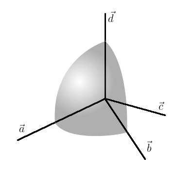

In the literature one finds two forms of the volume operator. These are the Rovelli-Smolin (RS) and Ashtekar-Lewandowski versions. The RS Rovelli & Smolin, 1994 version is
| (167) |
where is the alternating tensor.
The AL Ashtekar & Lewandowski, 1997 version is
| (168) |
Here is the orientation of the three tangent vectors at to the three curves/edges meeting at . The key difference between the two version lies in this term. The RS operator does not take into account the orientation of the edges which come into the vertex. This fact is taken into account in the AL version, and it allows us to speak of a phase transition from a state of geometry at high-temperature ()where the volume operator averages to zero for all graphs (which are “large” in some suitable sense) and a low-temperature () state where a geometric condensate forms and the volume operator gains a non-zero expectation value for states on all graphs. The key point here is that the AL version takes into account the “sign” of the volume contribution from any triplet of edges meeting at a vertex. Given any such triplet of edges , by flipping the orientation of any one edge we flip the sign of the corresponding contribution to . If we take the orientation of an edge as our random variable for the purposes of constructing a thermal ensemble, then it is clear that in the limit of high-temperature these orientations will flip randomly and the sum over the triplets of edges in will give zero for most (if not all) graph states. As we lower the temperature the system begins to anneal and for some temperature the system should reach a critical point where the volume operator spontaneously develops a non-zero expectation on most (if not all) graph states.
Note that;
- 1.
Since the result of the volume operator acting on a vertex depends on the signs of each triplet of edges, a simple dynamical system would then consist of a fixed graph with fixed spin assignments () to edges but with orientations that can flip, i.e. (much like a spin).
- 2.
The Hamiltonian must be a hermitian operator. This fixes the various term one can include in it. We must also include all terms consistent with all the allowed symmetries in our model.
- 3.
The simplest trivalent spin-network has one vertex with three edges, e.g. a vertex of the hexagonal lattice. One can generalize the action of the volume operator on graphs which have vertices with valence (number of connecting edges) greater than 3. (The volume operator gives zero on vertices with so these are excluded). To do so we use the fundamental identity which allows to decompose the state describing a vertex with into a sum over states with . One example of the decomposition of a four valent vertex into two three-valent vertices is in the following figure;

Figure 11: - 4.
This model can help us understand how a macroscopic geometry can emerge from the “spin” or many-body system described by a Hamiltonian, which contains terms with the volume and area operators, on a spin-network.
6.3 Spin Networks
This discussion leaves us with a simple mental picture of spin-networks. Briefly, they are graphs with representations (“spins”) of some gauge group (generally or in LQG) living on each edge. The links of this network correspond with cross-sectional areas, and the vertices where three or more links meet correspond with discrete volumes. The values of area and volume are determined by the spin labels on the relevant links. Since each link corresponds with the parallel transport of spin from one vertex to another, it is necessary to ensure that angular momentum is conserved at vertices, and so an intertwiner is associated with each vertex. For the case of a four-valent vertex we have four spins: . More generally a polyhedron with faces represents an intertwiner between the edges piercing each one of the faces. There is a simple visual picture of the intertwiner in the four-valent case.

Picture a tetrahedron enclosing the given vertex, such that each edge pierces precisely one face of the tetrahedron. Now, the natural prescription for what happens when a surface is punctured by a spin is to associate the Casimir of that spin with the puncture. The Casimir for spin has eigenvalues . These eigenvalues are identified with the area associated with a puncture.
In order for the edges and vertices to correspond to a consistent geometry it is important that certain constraints be satisfied. For instance, for a triangle we require that the edge lengths satisfy the triangle inequality and the angles should add up to , with if the triangle is embedded in a flat space and denoting the deviation of the space from zero curvature (positively or negatively curved).
In a similar manner, for a classical tetrahedron, now it is the sums of the areas of the faces which should satisfy “closure” constraints. For a quantum tetrahedron these constraints translate into relations between the operators which endow the faces with area.
For a triangle, giving its three edge lengths completely fixes the angles and there is no more freedom. However, specifying all four areas of a tetrahedron does not fix all the freedom. The tetrahedron can still be bent and distorted in ways that preserve the closure constraints. These are the physical degrees of freedom that an intertwiner possesses - the various shapes that are consistent with a tetrahedron with a given set of face areas.
6.4 Spin-Foams
In LQG the kinematical entities describing a given state of quantum geometry are spin-networks. The dynamical entities - i.e. those that encode the evolution and history of spin-networks - are known as spin-foams. If a spin-network describes a -dimensional spacelike geometry, then a spin-foam describes a possible history which maps this spin-network into another one. In order to determine the transition amplitudes between two different states of quantum-geometry whose initial and final states are given by spin-networks and , one must sum over all possible spin-foams which interpolate between the two spin-network states. When we perform the sum over all allowed histories we find that the resulting amplitude depends only on the boundary configuration of spins. This is holography. The holographic principle boils down to saying that the state of a system is determined by the state of its boundary. Therefore, although the point is not made as often is it possibly should be, LQG embodies the holographic principle in a very fundamental way. A spin-foam corresponds to a history which connects two spin-network states. On a given spin-network one can perform certain operations on edges and vertices which leave the state in the kinematical Hilbert space. These involve moves which split or join edges and vertices and those which change the connectivity. There are two basic transformations which the transitions between network states can be built from. These are the “2-to-2” move, in which an adjacent pair of trivalent vertices in a network exchange one incoming link each, and the “1-to-3” move, in which a single trivalent vertex splits into three vertices, in analogy to the “star-triangle transformation” used in the analysis of electrical circuits (see fig. 13). The inverse moves are also possible, of course, and the reader should easily recognize that the 2-to-2 move is its own inverse, while the inverse of the 1-to-3 move shrinks a trio of vertices down to form a single vertex.

One can “formally” view a spin-foam as a succession of states obtained by the repeated action of the scalar constraint
| (169) |
and so on Reisenberger, 1994; Reisenberger & Rovelli, 1997. It is not our intention to discuss spin-foams in great detail here. Hopefully the preceding material has sufficiently familiarized the reader with the notation and concepts of LQG that they will be able to read other, more specific discussions of spin-foams easily.
7 Applications
Ultimately, the value of any theory is judged by its relevance for the real world. Unfortunately, due to the small length scales involved, direct tests of models of quantum gravity are not easy to perform. However one can try to reproduce well-known results from other physical theories as a preliminary consistency test for newer theories. In this section, we will consider how LQG can be applied to the calculation of black hole entropy, and cosmological models.
While the question of black hole entropy is, as yet, an abstract problem, it is concrete enough to serve as a test-bed for theories of quantum gravity. In addition to the Bekenstein area law (mentioned in sec. 1), by investigating the behavior of a scalar field in the curved background geometry near a black hole horizon it was determined Hawking, 1975 that all black holes behave as almost perfect black bodies radiating at a temperature inversely proportional to the mass of the black hole: . This thermal flux is named Hawking radiation after its discoverer. These properties of a black hole turn out to be completely independent of the nature and constitution of the matter which underwent gravitational collapse to form the black hole in the first place. These developments led to the understanding that a macroscopic black hole, at equilibrium, can be described as a thermal system characterized solely by its mass, charge and angular momentum.
Bekenstein’s result has a deep implications for any theory of quantum gravity. The “Bekenstein bound” refers to the fact that eq. (1) is the maximum number of degrees of freedom - of both, geometry and matter - that can lie within any region of spacetime of a given volume . The argument is straightforward Susskind, 1994. Consider a region of volume whose entropy is greater than that of a black hole which would fit inside the given volume. If we add additional matter to the volume, we will eventually trigger gravitational collapse leading to the formation of a black hole, whose entropy will be less than the entropy of the region was initially. However, such a process would violate the second law of thermodynamics and therefore the entropy of a given volume must be at a maximum when that volume is occupied by a black hole. And since the entropy of a black hole is contained entirely on its horizon, one must conclude that the maximum number of degrees of freedom that would be required to describe the physics in a given region of spacetime , in any theory of quantum gravity, scales not as the volume of the region , but as the area of its boundary Hooft, 1993; Susskind, 1994 .
In view of the independence of the Bekenstein entropy on the matter content of the black hole, the origin of eq. (1) must be sought in the properties of the horizon geometry. Assuming that at the Planck scale, geometrical observables such as area are quantized such that there is a minimum possible area element that the black hole horizon, or any surface for that matter, can be “cut up into”, eq. (1) can be seen as arising from the number of ways that one can put (or “sew”) together quanta of area to form a horizon of area , where is a constant. In this manner, understanding the thermal properties of a black hole leads us to profound conclusions:
- 1.
In a theory of quantum gravity the physics within a given volume of spacetime is completely determined by the values of fields on the boundary of that region . This is the statement of the holographic principle.
- 2.
At the Planck scale (or at whichever scale quantum gravitational effects become relevant) spacetime ceases to be a smooth and continuous entity, i.e. geometric observables are quantized.
In LQG, the second feature arises naturally - though not all theorists are convinced that geometry should be “quantized” or that LQG is the right way to do so. One can also argue on general grounds that the first feature - holography - is also present in LQG, though this has not been demonstrated in a conclusive manner. Perhaps this paper might motivate some of its readers to close this gap!
Let us now review the black hole entropy calculation in the framework of LQG.
7.1 Black Hole Entropy
The ideas of quantum geometry allow us to give a statistical mechanical description of a black hole horizon. This is analogous to the statistical mechanical description of entropy for a gas, or some other system composed of many smaller parts, and can be illustrated by a toy model involving tossed coins.
Suppose we toss fair coins in succession, and record both the order of each series of heads and tails (this is called a microstate, since it keeps track of what each “particle” in the system does) and the total number of heads and tails that occur, ignoring the order (this is called the macrostate). In general, several microstates will correspond to a given macrostate. For instance, if , there is only one way to create a macrostate with zero heads (TTTT), or with four heads (HHHH), for the macrostate with three heads (and hence, one tail), there are four microstates (HHHT, HHTH, HTHH, and THHH), and similarly for the macrostate with one head and three tails. And for the macrostate with two heads and two tails there are six microstates. The number of microstates as a function of the number of heads in the macrostate, , follows a Gaussian distribution, which has the general form
| (170) |
where and and are scaling constants. Taking the natural logarithm of both sides we find that
| (171) |
We identify the left-hand side with the entropy of the specified macrostate, remembering that in general different macrostates will have different entropies3030 30 For a hand-waving argument as to why this should be the entropy, consider a simplified gas in which each molecule has just two speeds, (tails) and (heads). Then the variable is related to the average speed of the gas molecules, which when squared is related to their energy, and this may be related to entropy by the equation at constant .. The right-hand side is proportional to the logarithm of the number of microstates allowed in that macrostate. If we were interested in calculating the entropy of a gas, rather than tossing coins, the macrostates would correspond to particular values of pressure and temperature, while the microstates correspond to the positions and momenta of individual molecules.
In general there are two ways to calculate the entropy associated with a given random variable .
- 1.
Using Shannon’s formula. Let us say that we sample our random variable from some given ensemble, from which we draw samples. The variable takes values in the set where ), then the entropy associated with our lack of knowledge of the variable is given by:
(172) where is the probability that the random variable takes on the value . If in the samples on which the entropy is based, the value occurs times (with the constraint that ), then we have the usual frequentist definition for the probability associated with that value:
The definition of the Shannon entropy (172) is equivalent to the definition of the Gibbs entropy in statistical mechanics.
- 2.
Using the statistical mechanics method, or its more general version, Jaynes’ formalism Jaynes, 1957. This is based on the maximum entropy principle, according to which, in the absence of any prior information about a given random variable the least unbiased assumption one can make is that the variable satisfies a probability distribution which possesses the maximum possible entropy. This assumption leads us to the usual Boltzmann form of the probability. For a given value of the random variable , the associated probability distribution must satisfy the maximum entropy criterion (wherein (172) is maximized) and also the usual axioms of probability theory
(173a) (173b) where is any function of . The unique probability function which satisfies these criteria is found to be (see for e.g. Pathria & Beale, 2011, Sec. 3.2):
(174) where are Lagrange multipliers required for enforcing the constraints given in (173) 3131 31 The quantity being extremized has the form . can be identified with the chemical potential and the inverse temperature, respectively associated with the random variable . Using (174) we can write down the partition function
(175) given which we can evaluate the usual thermodynamic quantities such as expectation values, free energy and the entropy in :
(176a) (176b) (176c) where the inverse “temperature” is given by .
In the case of quantum geometry, the microstates correspond with the assignments of area to the discrete “pieces” of a surface (such as the event horizon of a black hole). Hence for each macroscopic interval of area , entropy is proportional to the log of the number of ways in which we can puncture the sphere to yield an area within that interval.

The state of a quantum surface is specified by a sequence of integers (or half-integers depending on the gauge group) , each of which labels an edge which punctures the given surface. The area of the surface is given by a sum over the Casimir at each puncture:
| (177) |
The eigenvalues of the operator are of the form , where . Thus, the eigenvalues of the area operator are of the form
| (178) |
In addition to (178) the integers must also satisfy a so-called projection constraint, which is discussed later in this section.
The task at hand is the following; given an interval , where is a macroscopic area value and is some small interval (), and the number of edges which puncture the surface, determine the allowed the number of sequences of integers , such that the resulting value for the total area falls within the given interval
| (179) |
There are various approaches to this problem. We summarize two of these - the simple argument of Rovelli’s Rovelli, 1996 and the number theoretical approach of Agullo et al., 2008; Agullo et al., 2011.
7.1.1 Rovelli’s Counting
We want to compute the number of sequences , where each sequence satisfies
Let us first note the following set of inequalities:
| (180) |
Let denote the number of sequences such that and denote the number of sequences such that ). Then the above set of inequalities implies that Rovelli, 1996
| (181) |
Computing boils down to counting the number of partitions of , i.e. the numbers of sets of ordered, positive integers whose sum is . As noted in Rovelli, 1996, this can be solved by observing that if is a partition of , then and are partitions of . All partitions of can be obtained in this manner and therefore we have , which implies that , where is a constant.
7.1.2 Number Theoretical Approach
This approach consists of two steps;
- A.
Determining allowed sequences. This involves solving the BP (Brahmagupta-Pell) equation3232 32 It is well-known that the name of “Pell’s Equation” was the result of Leonhard Euler’s misidentification of John Pell with the mathematician Lord Brouckner. If we gave Euler a second chance to name the equation, he might have called it “Brouckner’s equation”. This equation had previously been intensively studied by the Indian mathematicians Brahmagupta and Bhaskara around the 5 century B.C. and 12 century A.D. respectively. However, Brouckner and Euler are to be forgiven for not having knowledge of the existence of this earlier work. The authors hereby take the liberty of correcting this historical wrong associated with the naming of this equation, by adding the prefix “Brahmagupta” to the presently accepted name “Pell’s Equation”.. For now, we will work in units where . Thus for a given set of punctures on a quantum horizon, the total area can be written as
For each possible value of , let be the number of punctures which have that eigenvalue. So, we can write
with if no puncture has spin . As shown in Appendix G, the square root of any integer can be written as the product of an integer and the square-root of a square-free integer. Since , therefore we can write
for some and , where is the set of square-free integers. This implies that the area eigenvalue can be written as an integer linear combination of square-roots of square-free numbers:
leading us to the condition that
As a first step towards solving the general case, let us first try to determine the solution of the above equation for a single area eigenvalue :
knowing which we will be able to solve the general equation. Here the unknown variables are . The are the known square-free numbers. Setting and squaring both sides we obtain
This is commonly known as Pell’s equation, or perhaps more appropriately as the Brahmagupta-Pell equation. A method for obtaining its solutions is given in Appendix H.
- B.
Determining the number of valid ways of sprinkling labels from an allowed sequence onto the edges. This can be mapped to one of the simpler examples of NP-complete problems in the field of computational complexity - the Number Partitioning Problem Mertens, 1998; Mertens, 2000.
The relevance of the NPP for black hole entropy arises as follows. The counting of states of a horizon for a non-rotating black hole boils down to determining the number of ways in which we can choose spin-labels from a given sequence (where the allowed sequences are determined by solving the Brahmagupta-Pell equation) to each of the edges puncturing the horizon, such that .
More generally the case where , corresponds to a horizon with angular momentum . This is equivalent to the statement of the NPP, where given an arbitrary but fixed sequence of (positive) integers , one asks for the number of ways in which we can partition into two subsets and , such that the difference of the sum of the elements of each subset is minimized: . For the BHE problem is given by .
As shown in Agullo et al., 2008 this problem can be mapped to a non-interacting spin-system De˜Raedt et al., 2001 as follows. Consider a chain of spins each of which can be in an up state or a down state. If belongs to () then we set the spin to up (down). Consequently the constraint can be expressed as the condition that
(182) where are the possible eigenvalues of . The problem of partitioning is then equivalent De˜Raedt et al., 2001 to determining the ground state of the Hamiltonian
(183) where is the Pauli spin operator for the spin. Any eigenstate of with zero energy corresponds to a solution of the NPP for the set .
7.2 Loop Quantum Cosmology
One of the first avenues to follow when approaching old problems with new tools is to select the simplest possible scenarios for study, in the hope that the understanding gained in this arena would ultimately lead to a better understanding of more complex systems and processes. In classical GR this corresponds to studying the symmetry reduced solutions3333 33 That is, the solutions of the EFEs possessing strong global symmetries which reduces the effective local degrees of freedom to a small number. of Einstein’s equations, such as the FLRW cosmologies and their anisotropic counterparts, and various other exact solutions such as deSitter, anti-deSitter, Schwarzschild, Kerr-Newman etc.3434 34 We refer the reader to the extremely comprehensive and well-researched catalog of solutions to Einstein’s field equations, in both metric and connection variables, presented in Mueller & Grave, 2009. A somewhat older, but still valuable, catalog of exact solutions is given in Stephani et al., 2003. which correspond respectively to a “universe” (in this very restricted sense) with positive cosmological constant (), a universe with , a non-rotating black hole and a rotating black hole (both in asymptotically flat spacetimes3535 35 A metric with a radial dependence is considered asymptotically flat if it approaches (in a well-defined sense) a flat Minkowski metric as .). In each of these cases the metric has a very small number of local degrees of freedom and hence provides only a “toy model”. Of course, in the real world, the cosmos is a many-body system and reducing its study to a model such as the FLRW universe is a gross simplification. However, via such models, one can obtain a qualitative grasp of the behavior of the cosmos on the largest scales.
7.2.1 FLRW Models
The simplest quantum cosmological model is that which corresponds to the Friedmann metric whose line-element is given by3636 36 The following discussion is taken from Bojowald, 2006, Section 4.
| (184) |
where the only dynamical variable is the scale factor which depends only on the time parameter; is the radial dimension of the spatial slices; is the angular volume element and determines whether our spatial slices are open (), flat () or closed (). For this metric we can perform the decomposition and write down the action in terms of the various constraints. By comparing this metric with the general form given in eq. (83), we see that is the lapse function and the shift vanishes . This implies that the diffeomorphism constraint must also vanish.
Inserting this metric into the the EFE (13) gives us the vacuum Friedmann-LeMaitre-Robertson-Walker equations which describe the dynamics of homogenous, isotropic spacetimes:
| (185) |
where is the Hamiltonian for any matter fields that might be present. This equation gives us the Hamiltonian constraint for the FLRW metric. This can be seen by starting from the Lagrangian formulation where
| (186) |
The Ricci scalar for the FLRW line-element (184) is
| (187) |
Substituting the above into the we obtain
| (188) |
From this equation we can identify the momentum conjugate to the (only) degree of freedom - the scale factor :
| (189) |
Since the action does not contain any terms depending on , we have , implying that the lapse function is not a dynamical degree of freedom. We can now write down the Hamiltonian for the system in the usual manner: , which gives:
| (190) |
It is clear from the form of this expression that this Hamiltonian will become divergent as . Changing from metric to connection variables will allow us to alleviate this problem.
7.2.2 Connection Variables
For isotropic spacetimes, the triad and extrinsic curvature take the form Alexander & Vaid, 2006, Section IV:
| (191) |
In variables adapted to the particular form of the metric (184), the connection and triad are expressed as:
| (192) |
where is the Immirzi parameter. These components satisfy the commutation relations:
| (193) |
The factors of can be absorbed into the definition of the variables to give us:
| (194) |
In terms of these the Hamiltonian constraint (190) becomes:
| (195) |
where
7.3 Semiclassical Limit
The graviton propogator has a robust quantum version in these models. Its long-distance limit yields the behavior Rovelli, 2005 expected for gravity and an effective coarse-grained action given by the usual one consisting of the Ricci scalar plus terms containing quantum corrections.
8 Discussion and recent developments
Any fair and balanced review paper on LQG should also mention at least a few of the many objections its critics have presented. A list of a few of the more important points of weakness in the framework and brief responses to them follows:
- 1.
LQG admits a volume extensive entropy and therefore does not respect the Holographic principle: This criticism hinges upon the description of states of quantum gravity as spin-networks which are essentially spin-systems on arbitrary graphs. However, spin-networks only constitute the kinematical Hilbert space of LQG. They are solutions of the spatial diffeomorphism and the gauss constraints but not of the Hamiltonian constraint which generates time-evolution. This criticism is therefore due to a (perhaps understandable) failure to grasp the difference between the kinematical and the dynamical phase space of LQG.
In order to solve the Hamiltonian constraint we are forced to enlarge the set of states to include spin-foams which are histories of spin-networks. In a nutshell then, as we mentioned in sec. 6.4, the kinematical states of LQG are the spin-networks, while the dynamical states are the spin foams. The amplitudes associated with a given spin-foam are determined completely by the specification of its boundary state. Physical observables do not depend on the possible internal configurations of a spin-foam but only on its boundary state. In this sense LQG satisfies a stronger and cleaner version of holography than string theory, where this picture emerges from considerations involving graviton scattering from certain extremal black hole solutions.
- 2.
LQG violates the principle of local Lorentz invariance/picks out a preferred frame of reference: Lorentz invariance is obeyed in LQG but obviously not in the exact manner as for a continuum geometry. As has been shown by Rovelli and Speziale Rovelli & Speziale, 2010 the kinematical phase space of LQG can be cast into a manifestly Lorentz covariant form. A spin-network/spin-foam state transforms in a well-defined way under boosts and rotations. Similarly in quantum mechanics one finds that a quantum rotor transforms under discrete representations of the rotation group .
- 3.
LQG does not have stable semiclassical geometries as solutions - geometry “crumbles” - CDT simulations e.g. Loll et al., 2005 show how a stable geometry emerges. As mentioned in sec. 4.1, this involves calculating a sum over histories for the geometry of spacetime, between some initial and final state. The stability of the spacetimes studied in such simulations appears to be dependent on causality - that is, spacetime geometries develop unphysical structures in the Euclidean case, which are controlled when there is a well-defined past and future, as is the case in LQG. The question of exactly how similar CDT and LQG are to each other is a matter of continuing investigation.
- 4.
LQG does not contain fermionic and bosonic excitations that could be identified with members of the Standard Model: The area and volume operators do not describe the entirety of the structures that can occur within spin networks. LQG or a suitably modified version which allows braiding between various edges will exhibit invariant topological structures. Recent work Bilson-Thompson, 2005; Bilson-Thompson et al., 2007 has been able to identify some such structures with SM particles. In addition, in any spin-system - such as LQG - there are effective (emergent) low-energy degrees of freedom which satisfy the equations of motion for Dirac and gauge fields. Xiao-Gang Wen and Michael Levin Levin & Wen, 2004; Levin & Wen, 2007 have investigated so-called “string-nets” and find that the appropriate physical framework is the so-called “tensor category” or “tensor network” theory Biamonte et al., 2010; Evenbly & Vidal, 2011; Haegeman et al., 2011. In fact string-nets are very similar to spin-networks so Wen and Levin’s work - showing that gauge bosons and fermions are quasiparticles of string-net condensates - should carry over into LQG without much modification.
- 5.
LQG does not exhibit dualities in the manner String Theory does: Any spin-system exhibits dualities. A graph based model like LQG even more so. One example of a duality is to consider the dual of a spin-network which is a so-called 2-skeleton or simplicial cell-complex. Another is the star-triangle transformation, which can be applied to spin-networks which have certain symmetries, and which leads to a duality between the low and high temperature versions of a theory on a hexagonal and triangular lattice respectively Baxter, 2008.
- 6.
LQG doesn’t admit supersymmetry, wants to avoid extra dimensions, strings, extended objects, etc: Extra dimensions and supersymmetry are precisely that - “extra”. Occam’s razor dictates that a successful physical theory should be founded on the minimum number of ingredients. It is worth noting that at the time of writing of this paper, results from the LHC appear to have ruled out many supersymmetric extensions of the standard model. By avoiding the inclusion of extra dimensions and supersymmetry, LQG represents a perfectly valid attempt to create a theory that is consistent with observations.
- 7.
LQG has a proliferation of models and lacks robustness: Again a lack of extra baggage implies the opposite. LQG is a tightly constrained framework. There are various uniqueness theorems which underlie its foundations and were rigorously proven in the 1990s by Ashtekar, Lewandowski and others. There are questions about the role of the Immirzi parameter and the ambiguity it introduces however these are part and parcel of the broader question of the emergence of semi-classicality from LQG (see Simone Mercuri’s papers in this regard).
- 8.
LQG does not contain any well-defined observables and does not allow us to calculate graviton scattering amplitudes: Several calculations of two-point correlation functions in spin-foams exist in the literature Rovelli, 2005 These demonstrate the emergence of an inverse-square law.
As well as discussing criticisms of LQG, it is also fair to consider what role this theory may have in the future. We would not have written a paper reviewing the formulation and current status of LQG if we did not consider it an important and interesting theory - one which we feel is probably a good representation of the nature of spacetime. However it is wise to remember that most physical theories are ultimately found to be flawed or inadequate representations of reality, and it would be unrealistic to think that the same might not be true of LQG. Questions linger about the nature of time and the interpretation of the hamiltonian constraint, among other things. What is the value then, in studying LQG? Perhaps LQG will eventually be shown to be untenable, or perhaps it will be entirely vindicated. As authors of this paper, we feel that the truth will probably lie somewhere in the middle, and that however much of our current theories of LQG survive over the next few decades, this research program does provide strong indications about what some future (and, we hope, experimentally validated) theory of “Quantum Gravity” will look like.
Acknowledgements.
DV would like to thank SBT for invitations to visit the Perimeter Institute in Fall 2009, where this collaboration was born, and to visit the University of Adelaide in August, 2011 where this project was continued. DV also thanks the Perimeter Institute and the University of Adelaide for their hospitality during these visits. SBT would like to thank the Ramsay family for their support through the Ramsay Postdoctoral Fellowship. Finally, a special note of thanks is due to Martin Bojowald, without whose help this work would not have stayed true to its claim of being “self-contained”.Appendix A Conventions
Uppercase letters are “internal” indices which take values in the Lorentz lie-algebra. Greek letters are four-dimensional spacetime indices. Lowercase letters from the middle of the alphabet will be used for indices in a space of dimensions, lie-algebra indices, etc. Lowercase letters from the start of the alphabet are three-dimensional spatial indices.
A.1 Lorentz Lie-Algebra
The generators of the -dimensional representation of the Lorentz Lie algebra can be written in terms of the () Dirac gamma matrices , which satisfy the anticommutation relations
| (196) |
where is the metric tensor and is the identity matrix.
For the case of , the matrices are given by
where and are the usual Pauli matrices, and in this case is equivalent to , the usual Minkowski metric.
In terms of the , the generators of the Lorentz group can be written as Peskin & Schroeder, 1995
| (201) |
Note that, whereas in the above we have restricted ourselves to the case of dimensions, the expression for the generators of the Lorentz group goes through in any dimension, with either Lorentzian or Euclidean metric Peskin & Schroeder, 1995, Section 3.2. An -valued connection can then be written as
| (202) |
but by the antisymmetry of the gamma matrices, the above expression can be shortened to , where we remember that the connection is antisymmetric in the internal indices .
Appendix B Lie Derivative
The Lie derivative of a tensor is the change in evaluated along the flow generated by the vector field on a manifold. When is simply a function on the manifold, the Lie derivative reduces to the directional derivative of along 3737 37 this fact is related to the interpretation of the differential as a component of a 1-form, and the derivative operator as a component of a vector field:
where co-ordinatizes the points along the curve genereted by . When the connection is torsion-free, we may replace with .
It can be shown Wald, 1984 that:
| (203) |
where is shorthand for an expression with in the position and (s) or (s) elsewhere, e.g. . In particular the Lie derivative of a vector field along a vector field reduces to the commutator of the two vector fields:
| (204) |
In the case of a rank-2 tensor :
| (205) |
Applying this to the metric tensor we find the relation:
| (206) |
since the covariant derivative of the metric vanishes.
Appendix C ADM Variables
One would like to be able to determine the data required to embed the spatial hypersurfaces within the 4-manifold , given the spacetime metric & the unit time-like vector field normal to . This data consists of the intrinsic & extrinsic curvature tensors . As explained in the main text the object defined by 84 plays the role of the intrinsic metric (or “curvature”) of . The quantity is the extrinsic curvature of determined by the particular form its embedding in . In order to define we first need to determine the form of the covariant spatial derivative.
C.1 Covariant Spatial Derivative
The covariant spatial derivative on acting on purely spatial object is given by Bojowald, 2011, Sec. 3.2.2.2:
| (207) |
where is an arbitrary spacetime tensor. The spatial derivative of an arbitrary vector field can then be written as:
| (208) |
using the fact that because is a unit vector .
There is nothing mysterious about 208. It simply measures how the vector field changes from point to point as we move around the spatial manifold . To help visualize this one can think of an arbitrary configuration of the electric field in three-dimensional space . For simplicity, if is and is the surface , then the three-dimensional derivative operator on reduces to the two-dimensional derivative on the plane. tells us how changes as we move from one point to another in .
C.2 Extrinsic Curvature
The extrinsic curvature of a given manifold is a mathematical measure of the manner in which it is embedded in a manifold of higher dimension. As illustrated in 8b, a two-dimensional cylinder embedded in has zero instrinsic curvature, but non-zero extrinsic curvature. The normal at each point of the cylinder is a three-dimensional vector and this vector changes as one moves around the cylindrical surface if the extrinsic curvature of the surface is non-zero. Thus, the simplest definition for a tensorial quantity which measures this change is given by:
| (209) |
where is the covariant spatial derivative defined in C.1. This quantity turns out to be symmetric. In order to see this (Bojowald, 2011, Sec. 3.2.2.2), note that given two spatial vector fields and , their commutator will also be spatial, i.e. . This implies:
using the fact that since , and similarly for the remaining term. And since are purely spatial, this implies that (the spatial projection of) .
Thus the extrinsic curvature of can be written as:
| (210) |
C.3 Canonical Momentum in ADM Formulation
Recall that the time vector field is written in terms of the lapse , shift and the normal to the hypersurface , so that (eq. (79)). We wish to write down the explicit form of the Lie-derivative of a one-index and two-index object , with respect to a vector field . Conveniently this is already present in equations (204)…(206)! As we may expect, when a vector field is a sum of two (or more) vector fields (as for the time-evolution field above), the Lie derivative with respect to that field decomposes into the sum of Lie derivatives with respect to each of the components fields. So if , then , where is the arbitrary tensor whose Lie derivative we want to find. You can see this directly from eq. (203) by writing the field X as a sum of other vector fields. When, is a vector, then and so on ( is the commutator of two vector fields as in eq. (204)).
There are two steps involved in deriving the form of the canonical momentum. First is to prove the identity (93). The second is to use that result to perform the functional derivative of the Einstein-Hilbert Lagrangian w.r.t. the to obtain eq. (94).
First, we wish to show that , which we can do by finding a suitable expression for , and then restricting the indices to the range . So, since , using the above mentioned additive property of Lie derivatives, we have . The second term is present unchanged in eq. (93). Now it remains to be shown that .
In the following we follow the treatment of Bojowald, 2011, Sec. 3.2.2.2. First we show that . Using the definition of the Lie derivative, we have:
| (211) |
where in the second and third lines we have used the expression for the spatial metric in terms of the four-metric and the unit normal to . In the third line the term containing is zero. In the third and fourth lines metric compatibility () is used to commute the 4-metric through the spacetime derivative. In the fifth line we have again used metric compatibility to write as , etc. .
For the last step we have need which finally yields:
| (212) |
All this algebra is not necessary if one notes that the Lie derivative of a metric tensor is given by 206, which we restate for convenience:
Now, note that the above equation holds true only when the derivative operator is compatible () with the metric whose Lie derivative we wish to determine. Hence we should use the correct notation for the spatial derivative operator instead of . Then we have:
| (213) |
which, by definition 210, is twice the extrinsic curvature of . Given this expression we proceed as follows:
| (214) |
where in the first line we have used 210 alongwith the definition 205 of the Lie derivative. In the second we have multiplied & divided by the scale factor . In the third we have used the fact that to move inside the derivative operator. In going from the third to the fourth, we have used the relationship between the lapse, shift and time-evolution fields: , followed by 205 (in reverse) and then used the linearity of the Lie derivative. In the fifth we have, in the words of Bojowald Bojowald, 2011, “smuggled in” two factors of knowing that is spatial to begin with. In the sixth, the spatial projection is identified as the “time-derivative” of the spatial metric. We leave the remaining step (to show that ) as an exercise for the reader.
To summarize, we have:
| (215) |
Now, the Einstein-Hilbert Lagrangian is given by:
The first term does not contain any dependence on or and so its derivative w.r.t. vanishes. For the remaining two terms we have:
here . can be written as :
| (216) |
From (215) we have:
| (217) |
Inserting this into the previous expression we have:
| (218) |
which is identical to (94) as desired.
Appendix D Duality
The notion of self-/anti-self-duality of the gauge field is central to understanding both the topological sector of Yang-Mills theory and the solutions of Einstein’s equations in the connection formulation. As discussed in sec. 3.2, the use of multivectors and -forms can be very helpful for understanding duality. Let us review these concepts.
D.1 Multivectors and Differential Forms
A vector is a directed line segment with a magnitude which is interpreted as a length. One way to form the product of two vectors and is the dot product , which is a scalar that is maximised when the vectors are parallel. We can also form the wedge product, , which is a directed surface spanned by and (the direction being both an orientation in space and a preferred direction of rotation around the boundary of the surface), with a magnitude interpreted as the area of the surface. This area is called a bivector, and its magnitude is maximised when and are perpendicular (and zero when they are parallel). The wedge product of three non-coplanar vectors is a trivector, which is a parallelipiped with a direction (a preferred directed path around the edges of the parallelipiped) and a magnitude interpreted as its volume. The wedge product of vectors (assuming they are not parallel, coplanar, etc.) will in general be called a multivector, being an oriented parallelipiped in dimensions, with a magnitude given by its enclosed volume. A scalar may be regarded as a -vector. We can define the Clifford product of multivectors as
| (219) |
If and are ordinary vectors, then if and are perpendicular since in this case . Hence when dealing with orthonormal basis vectors we may adopt the notation , and likewise , etc. Conversely if and are parallel then since in this case , hence .
The importance of multivector quantities in physics can be seen if we consider the case of four-dimensional Minkowski spacetime, where the scalar product is taken using the metric . Hence , and . In this case the basis vectors are isomorphic to the Dirac gamma matrices, , and the reader can verify that they satisfy , the defining relation of the Dirac matrices (see eq. (196)). Since this anticommutator is formed by taking Clifford products of the , the gamma matrices are said to generate a representation of a Clifford algebra.
Differential forms and multivectors can be seen to correspond closely. A bivector and a 2-form both define a plane. A trivector and a 3-form both define a volume, etc. However as mentioned in sec. 3.2, multivectors can be easier to visualise, as the magnitude of a -form is a density, while the magnitude of a multivector is a -dimensional volume. It can therefore often be easier to think of how the wedge products and duals of -forms behave by visualising them as multivectors.
Duality is a notion that emerges naturally from the construction of the space of multivectors, and likewise from the construction of the space of differential forms on a -dimensional manifold . Let denote the subspace consisting only of forms of order in dimensions e.g. in three dimensions the space of two-forms is spanned by the basis where is some local coordinate patch - i.e. a mapping from a portion of the given manifold to a region around the origin in .
Now one can show Baez & Muniain, 1994; Wald, 1984 that , i.e. the space of -forms is the same as the space of ()-forms. Thus any -form , defined on an dimensional manifold, can be mapped to an ()-form . This is accomplished with the completely antisymmetric tensor on :
| (220) |
This expression may appear daunting, but as suggested we can make its meaning clearer by examining duality with multivectors. Consider the case of three dimensions. The antisymmetry of the wedge product means that the unit trivector picks up a factor of each time the order of any two of its factors is swapped, hence , etc. and so the unit trivector is a geometrical representation of the antisymmetric tensor .

Multiplying a vector by the unit trivector yields a bivector, and multiplying a bivector by the unit trivector yields a vector (Figure 15). To see why, consider the familiar cross product. Any two, non-degenerate, vectors span a two-dimensional subspace of . Using these two vectors we construct a third vector , where the components of are given by . This construction is taught to us in elementary algebra courses, but never quite seemed to make complete sense because it seemed to be peculiar to three-dimensions. The product is a vector which is perpendicular to the plane defined by the vectors and . But this plane is the same one that the wedge product lies in. If we take the Clifford product of with the unit 3-vector, we are left with a vector that is perpendicular to the plane of , and which equals . Why? Because the components of the vector (bivector) parallel with components of the unit trivector yield scalars, leaving only the components perpendicular to , as we can see by expanding the Clifford product in full
| (221) | |||||
where in the second-last line we have used to rearrange the basis vector terms, so as to eliminate extra terms by using . We also find that the wedge product of and has components .
This allows us to view the cross product as a three-dimensional special case of a procedure that can be performed in any number of dimensions. This procedure is “forming the dual”. We can say that the cross product of two vectors is the dual of the wedge product, . In the language of differential forms this procedure is described by eq. (220), and utilises the antisymmetric tensor . In the language of multivectors, it involves taking the Clifford product with the unit multivector .
From now on we will speak of -forms, rather than -forms and/or multivectors. But their equivalence, and the geometric interpretation arising from this, should be kept in mind.
D.2 Spacetime Duality
From the discussion in sec. D.1, it should be obvious that in four dimensions the dual of any two-form is another two-form
| (222) |
(compare this with eq. (48), and as noted there, the quantity defined on the plane between any pair of spacetime axes is associated to the quantity defined on the plane between the other two spacetime axes). It is due to this property of even-dimensional manifolds that we can define self-dual and anti-self-dual -forms, where a form is self-/anti-self-dual if:
| (223) |
Given an arbitrary 2-form its self-dual part and anti-self-dual part are given by
where and are constants we have introduced for later convenience. We can check that
| (224) |
because in a Euclidean background. In other words and , which is precisely the definition of (anti-)self-duality. Thus any 2-form can always be written as a linear-sum of a self-dual and an anti-self-dual piece
The above results hold for a Euclidean spacetime. For a Lorentzian background we would instead have and the dual of a two-form is given by:
| (225) |
and the statement of (anti-)self-duality becomes
| (226) |
with the self-dual and anti-self-dual pieces of a two-form given by and
D.3 Lie-algebra duality
The previous section discussed self-duality in the context of tensors with spacetime indices . In gauge theories based on non-trivial Lie-algebras we also have tensors with lie-algebra indices, such as the curvature of the gauge connection where label generators of the relevant Lie algebra.. The dual of the connection can then be defined using the completely antisymmetric tensor acting on the Lie algebra indices, as in:
| (227) |
D.4 Yang-Mills
Let us illustrate the utility of the notion of self-duality by examining the classical Yang-Mills action:
Varying this action with respect to the connection gives us the equations of motion:
which are satisfied if , i.e. if the gauge curvature is self-dual or anti-self-dual. Thus for self-/anti-self-dual solutions the Yang-Mills action reduces to:
which is a topological invariant of the given manifold and is known as the Pontryagin index. Here the superscript on the r.h.s. denotes whether the field is self-dual or anti-self-dual.
D.5 Geometrical interpretation
Given any (Lie-algebra valued) two-form (where are Lie-algebra indices) we can obtain an element of the Lie-algebra by contracting it with a member of the basis of the space of two-forms: where denotes the vector and not the components of a vector. The components are suppressed in the differential form notation as explained in the preceding sections. The resulting lie-algebra element is
and is the flux of the field strength through the two-dimensional surface spanned by .
We can also define
which implies that , i.e. the flux of the field strength through the plane is equal to the flux of the dual field through the plane.
D.6 (Anti) Self-dual connections
When we say that the connection is (anti-)self-dual, explicitly this means that
| (228) |
Let us now show the relation between the (anti-)self-dual four-dimensional connection and its restriction to the spatial hypersurface . We begin by writing the full connection in terms of the generators of the Lorentz lie-algebra: and expanding the sum (see Alexander & Vaid, 2006, Section 2 and A.1):
In the second line we have used the fact that is antisymmetric in the internal indices and that the gamma matrices anticommute. In the third we have used the expressions for the gamma matrices given in Appendix A.1 to expand out the matrix products. This allows us to write the last line in the above expression in the form
where:
| (236a) | ||||
| (236b) | ||||
For , using the definition of the dual connection, we find that
and so we may rewrite these expressions as
| (237a) | ||||
| (237b) | ||||
Appendix E Path Ordered Exponential
From eq. (52) we see that the effect of a holonomy of a connection along a path (for either an open or closed path) in a manifold is defined as
| (238) |
The exponential can be formally expressed in terms of a Taylor series expansion:
| (239) |
where for the term in the sum, the path is broken up into intervals parametrized by the variables over which the integrals are performed. The path ordering enforces the condition that the effect of traversing each interval is applied the order that the intervals occur. The interested reader is referred to pgs. 66 - 68 of Carroll, 1997.
Appendix F Peter-Weyl Theorem
The crucial step involved in going from graph states with edges labelled by holonomies to graph states with edge labelled by group representations (angular momenta) is the Peter-Weyl theorem . This theorem allows the generalization of the notion of Fourier transforms to functions defined on a group manifold for compact, semi-simple Lie groups.
Given a group , let be the matrix representation of any group element . Then we have (see Chapter 8 of Tung & Tung, 1985):
Theorem F.1.
The irreducible represenation matrices for the group satisfy the following orthonormality condition
| (240) |
Here is the dimensionality of the representation of and is the order of the group. For a finite group this is simply the number of elements of the group. For example, for , . However a continuous or Lie group such as has an uncountable infinity of group elements. In such cases corresponds to the “volume” of the group manifold.
This property allows us to decompose any square-integrable function in terms of its components with respect to the matrix coefficients of the group representations:
Theorem F.2.
The irreducible representation functions form a complete basis of (Lebesgue) square-integrable functions defined on the group manifold.
Any such function can then be expanded as
| (241) |
where are constants which can be determined by inserting the above expression for in 240 and integrating over the group manifold. Thus we obtain
| (242) | |||||
which gives us
| (243) |
Appendix G Square-Free Numbers
According to the fundamental theorem of arithmetic, any integer , has a unique factorization in term of prime numbers:
where are the prime-numbers which divide , one or more times. is the number of times the prime number occurs in the factorization of . Thus, we have:
We can partition the set into two sets containing only the even or odd elements respectively
where , , and . This gives:
Since each of the and , for some , we have:
It is evident that since the third term in the product has no repeating elements, its square-root cannot be an integer (i.e. the presence of repeating elements would lead to an expression like ). Such an integer , in therefore known as a square-free integer. Thus any integer can be written as the product of a square-free integer () and another (non square-free) integer such that .
Appendix H Brahmagupta-Pell Equation
Around the 7 century A.D. the Indian mathematician Brahmagupta, demonstrated the Brahmagupta-Fibonacci Identity,
| (244) | |||||
| (245) |
where we have added and subtracted from the l.h.s. on the first line. The above goes through for all . Given any pair of triples of the form , where , which are solutions of the Diophantine equation , we can construct a third triple , which is also a solution of the same equation, by applying the Brahmagupta-Fibonacci identity to the first two pairs
| (246) |
which tells us that , and . One can easily check that the triple is also a solution of the Diophantine equation.
When we apply the restriction that , the Diophantine equation reduces to the Brahmagupta-Pell equation,
and given two pairs of solutions to the BP equation (for the same fixed value of ), we can generate a third solution given by . More generally given any solution to the BP equation, one can generate an infinite set of solutions by repeatedly applying the BF identity to the starting solution
| (247) |
Here, the pair is referred to as the fundamental solution.
H.1 Quadratic Integers and the BP Equation
We are familiar with solutions of equations of the form
This is the quadratic equation from beginning algebra courses, which has as solutions
when the discriminant is negative, the roots of the equation are imaginary or complex numbers
where and . When , the solutions of the quadratic equations can be characterized as elements of the field of quadratic integers , which is an extension of the familiar field of rational numbers . Such numbers have the form
where , if and otherwise (if ). , where is the set of square-free integers.
It is at this point that one makes a connection to the square-free quadratic extension of the field of rationals and its integral subset , by noting that any solution of the BP equation can be represented as a quadratic integer:
The consistency of this representation is enforced by the fact that the multiplication law for two quadratic integers is the same condition satisfied when multiplying two pairs of solutions of the BP equation to obtain a third pair, i.e. , if and are two members of , then their product is given by:
| (248) | ||||
| (249) |
which is identical to the multiplication law satisfied by pairs of solutions of the BP equation.
Appendix I Kodama State
The Kodama state is an exact solution of the Hamiltonian constraint for LQG with positive cosmological constant and hence is of great importance for the theory. It is given by
| (250) |
where is a normalization constant. The action is the Chern-Simons action for the connection on the spatial 3-manifold , given by
where
with being the exterior derivative. Consistent with our discussion of bivectors and -forms in sec. D.1 the wedge product between two 1-forms and is:
For identical one-forms the wedge product gives zero. That is why for the Chern-Simons action to have a non-zero cubic term the connection must be non-abelian. Let us write the various terms in the Chern-Simons density explicitly;
where are worldvolume (“spacetime”) indices, are worldsheet (“internal”) indices and are the basis vectors of the lie-algebra/internal space.
Taking the trace over these terms gives us
The trace over the lie-algebra elements gives us:
where are the structure constants of the gauge group.
Appendix J 3j-symbols
The Wigner 3j-symbol is related to the Clebsch-Gordan coefficients through:
where the are the orbital and magnetic quantum numbers of the particle. is the state representing two particles (or systems) each with their separate angular momentum numbers. represents the total angular momentum of the system. Classically we have two systems with angular momentum and , then the angular momentum of the combined system is: .
In quantum mechanics, however, the angular momentum of the composite system can be any one of a set of possible allowed choices. Whether or not the angular momentum of the composite system can be specified by quantum numbers is determined by whether or not the Clebsch-Gordan coefficient is non-zero.
Appendix K Regge Calculus
Regge showed in 1961 that one could obtain the continuum action of general relativity “in 2+1 dimensions” from a discrete version thereof given by decomposing the spacetime manifold into a collection of tetrahedral simplices Regge, 1961; Iwasaki, 1994. When many such tetrahedra are joined together, curvature of the resulting discrete manifold is represented by positive or negative deficit angles (for instance, a plane 2D surface can be tiled with equilateral triangles, with six such triangles meeting at each vertex. If one attempted to increase the number of degrees round a given vertex by fitting a seventh triangle in, the only way it could be accommodated would be by curving the resulting surface).
| (251) |
is the Regge action for the tetrahedron. Here the sum over is the sum over the edges of the tetrahedron. and are the length of the edge and the dihedral deficit angle, respectively, around the edge of the tetrahedron.
The Regge action for a manifold built up by gluing such simplices together is simply the sum of the above expression over all simplices
It was later shown by Ponzano and Regge Ponzano & Regge, 1968 that in the limit, the 6-j symbol corresponds to the cosine of the Regge action Regge & Williams, 2000
References
- Gaul & Rovelli (1999) Marcus Gaul and Carlo Rovelli “Loop Quantum Gravity and the Meaning of Diffeomorphism Invariance”, 1999 arXiv: http://arxiv.org/abs/gr-qc/9910079v2
- Ashtekar & Lewandowski (2004) Abhay Ashtekar and Jerzy Lewandowski “Background independent quantum gravity: a status report” In Classical and Quantum Gravity 21.15, 2004, pp. R53–R152 DOI: 10.1088/0264-9381/21/15/R01
- Kiefer (2005) Claus Kiefer “Quantum Gravity: General Introduction and Recent Developments”, 2005 arXiv: http://arxiv.org/abs/gr-qc/0508120
- Nicolai & Peeters (2006) Hermann Nicolai and Kasper Peeters “Loop and spin foam quantum gravity: a brief guide for beginners”, 2006 DOI: 10.1007/978-3-540-71117-9˙9
- Alexandrov & Roche (2010) Sergei Alexandrov and Philippe Roche “Critical Overview of Loops and Foams”, 2010 arXiv: http://arxiv.org/abs/1009.4475
- Mercuri (2010) Simone Mercuri “Introduction to Loop Quantum Gravity”, 2010 arXiv: http://arxiv.org/abs/1001.1330
- Don“’a & Speziale (2010) Pietro Don“’a and Simone Speziale “Introductory lectures to loop quantum gravity”, 2010 arXiv: http://arxiv.org/abs/1007.0402
- Esposito (2011) Giampiero Esposito “An introduction to quantum gravity”, 2011 arXiv: http://arxiv.org/abs/1108.3269
- Rovelli (2011) Carlo Rovelli “Zakopane Lectures on loop gravity”, 2011 arXiv: http://arxiv.org/abs/1102.3660
- Ashtekar (2012) Abhay Ashtekar “Introduction to Loop Quantum Gravity”, 2012 arXiv: http://arxiv.org/abs/1201.4598
- Perez (2012) Alejandro Perez “The new spin foam models and quantum gravity”, 2012 arXiv: http://arxiv.org/abs/1205.0911
- Bekenstein (1972) J. Bekenstein “Black holes and the second law” In Lettere Al Nuovo Cimento (1971 – 1985) 4.15 Italian Physical Society, 1972, pp. 737–740 DOI: 10.1007/BF02757029
- Bekenstein (1973) Jacob˜D. Bekenstein “Black Holes and Entropy” In Physical Review D 7.8 American Physical Society, 1973, pp. 2333–2346 DOI: 10.1103/PhysRevD.7.2333
- Bekenstein (1973a) J.˜D. Bekenstein “Extraction of energy and charge from a black hole” In Phys. Rev. D7, 1973, pp. 949–953
- Wald (1984) Robert˜M. Wald “General Relativity” The University of Chicago Press, 1984
- Koks (2006) D. Koks “Explorations in Mathematical Physics: The Concepts Behind an Elegant Language” Springer, 2006
- Moriyasu (1983) K. Moriyasu “An elementary primer for gauge theory” World Scientific, 1983
- Peskin & Schroeder (1995) M.˜E. Peskin and D.˜V. Schroeder “An Introduction to Quantum Field Theory” Addison Wesley, 1995
- Hobson et al. (2006) M.˜P. Hobson, G.˜P. Efstathiou and A.˜N. Lasenby “General Relativity: An Introduction for Physicists” Cambridge University Press, 2006
- Loll et al. (2005) Renate Loll, J. Ambjorn and J. Jurkiewicz “The Universe from Scratch”, 2005 eprint:hep-th/0509010
- Romano (1993) Joseph˜D. Romano “Geometrodynamics vs. Connection Dynamics”, 1993 DOI: 10.1007/BF00758384
- Ashtekar (1991) A. Ashtekar “Lectures on non-perturbative canonical gravity” In Advanced Series in Astrophysics and Cosmology, Singapore: World Scientific, 1991, 1991 URL: http://adsabs.harvard.edu/cgi-bin/nph-bib_query?bibcode=1991lnpc.book.verb....A
- Thiemann (2001) Thomas Thiemann “Introduction to Modern Canonical Quantum General Relativity”, 2001 arXiv: http://arxiv.org/abs/gr-qc/0110034
- Peldan (1993) Peter Peldan “Actions for Gravity, with Generalizations: A Review”, 1993 arXiv: http://arxiv.org/abs/gr-qc/9305011
- D’Inverno (1992) R. D’Inverno “Introducing Einstein’s Relativity” Oxford University Press, 1992
- Jacobson & Smolin (1988) T. Jacobson and L. Smolin “Covariant action for Ashtekar’s form of canonical gravity” In Classical and Quantum Gravity 5.4, 1988, pp. 583+ DOI: 10.1088/0264-9381/5/4/006
- Samuel (1987) Joseph Samuel “A lagrangian basis for ashtekar’s reformulation of canonical gravity” In Pramana 28.4 Springer India, in co-publication with Indian Academy of Sciences, 1987, pp. L429–L432 DOI: 10.1007/BF02847105
- Ashtekar & Lewandowski (1996) Abhay Ashtekar and Jerzy Lewandowski “Differential Geometry on the Space of Connections via Graphs and Projective Limits”, 1996 arXiv: http://arxiv.org/abs/hep-th/9412073
- Ashtekar & Lewandowski (1996a) Abhay Ashtekar and Jerzy Lewandowski “Quantum Theory of Gravity I: Area Operators”, 1996 arXiv: http://arxiv.org/abs/gr-qc/9602046
- Ashtekar & Lewandowski (1997) Abhay Ashtekar and Jerzy Lewandowski “Quantum Theory of Geometry II: Volume operators”, 1997 arXiv: http://arxiv.org/abs/gr-qc/9711031
- Ashtekar et al. (1999) A. Ashtekar, A. Corichi and K. Krasnov “Isolated Horizons: the Classical Phase Space”, 1999 arXiv: http://arxiv.org/abs/gr-qc/9905089
- Ashtekar et al. (2000) A. Ashtekar, J. Baez and K. Krasnov “Quantum Geometry of Isolated Horizons and Black Hole Entropy”, 2000 arXiv: http://arxiv.org/abs/gr-qc/0005126
- Rovelli & Smolin (1994) Carlo Rovelli and Lee Smolin “Discreteness of area and volume in quantum gravity”, 1994 arXiv: http://arxiv.org/abs/gr-qc/9411005
- Reisenberger (1994) Michael Reisenberger “Worldsheet formulations of gauge theories and gravity”, 1994 URL: http://arxiv.org/abs/gr-qc/9412035
- Reisenberger & Rovelli (1997) Michael˜P. Reisenberger and Carlo Rovelli ““Sum over Surfaces” form of Loop Quantum Gravity”, 1997 URL: http://arxiv.org/abs/gr-qc/9612035
- Hawking (1975) S. Hawking “Particle creation by black holes” In Communications in Mathematical Physics 43.3, 1975, pp. 199–220 DOI: 10.1007/BF02345020
- Susskind (1994) L. Susskind “The World as a Hologram” In Journal of Mathematical Physics 36.11 AIP, 1994, pp. 6377–6396 DOI: 10.1063/1.531249
- Hooft (1993) G. Hooft “Dimensional Reduction in Quantum Gravity”, 1993 arXiv: http://arxiv.org/abs/gr-qc/9310026
- Jaynes (1957) E.˜T. Jaynes “Information Theory and Statistical Mechanics” In Physical Review Online Archive (Prola) 106.4 American Physical Society, 1957, pp. 620–630 DOI: 10.1103/PhysRev.106.620
- Pathria & Beale (2011) R.˜K. Pathria and Paul˜D. Beale “Statistical Mechanics, Third Edition” Academic Press, Paperback, 2011 URL: http://www.amazon.com/exec/obidos/redirect?tag=citeulike07-20&path=ASIverbN/0123821886
- Rovelli (1996) Carlo Rovelli “Black Hole Entropy from Loop Quantum Gravity”, 1996 DOI: 10.1103/PhysRevLett.77.3288
- Agullo et al. (2008) Ivan Agullo et al. “Black hole state counting in Loop Quantum Gravity: A number theoretical approach” In Physical Review Letters 100.21, 2008 arXiv: http://arxiv.org/abs/0802.4077
- Agullo et al. (2011) Ivan Agullo et al. “Detailed black hole state counting in loop quantum gravity”, 2011 arXiv: http://arxiv.org/abs/arXiv:1101.3660
- Mertens (1998) Stephan Mertens “Phase Transition in the Number Partitioning Problem” In Physical Review Letters 81.20, 1998, pp. 4281–4284 DOI: 10.1103/physrevlett.81.4281
- Mertens (2000) Stephan Mertens “A physicist’s approach to number partitioning”, 2000 arXiv: http://arxiv.org/abs/cond-mat/0009230
- De˜Raedt et al. (2001) H. De˜Raedt, K. Michielsen, K. De˜Raedt and S. Miyashita “Number Partitioning on a Quantum Computer”, 2001 arXiv: http://arxiv.org/abs/quant-ph/0010018
- Mueller & Grave (2009) Thomas Mueller and Frank Grave “Catalogue of Spacetimes”, 2009 arXiv: http://arxiv.org/abs/arxiv:0904.4184
- Stephani et al. (2003) Hans Stephani et al. “Exact Solutions of Einstein’s Field Equations (Cambridge Monographs on Mathematical Physics)” Cambridge University Press, Hardcover, 2003 URL: http://www.amazon.com/exec/obidos/redirect?tag=citeulike07-20&path=ASIverbN/0521461367
- Bojowald (2006) Martin Bojowald “Loop Quantum Cosmology”, 2006 arXiv: http://arxiv.org/abs/gr-qc/0601085
- Alexander & Vaid (2006) Stephon H.˜S. Alexander and Deepak Vaid “Gravity Induced Chiral Condensate Formation and the Cosmological Constant”, 2006 arXiv: http://arxiv.org/abs/hep-th/0609066
- Rovelli (2005) Carlo Rovelli “Graviton propagator from background-independent quantum gravity”, 2005 DOI: 10.1103/PhysRevLett.97.151301
- Rovelli & Speziale (2010) Carlo Rovelli and Simone Speziale “Lorentz covariance of loop quantum gravity”, 2010 arXiv: http://arxiv.org/abs/1012.1739
- Bilson-Thompson (2005) S.˜O. Bilson-Thompson “A topological model of composite preons”, 2005 eprint:hep-ph/0503213
- Bilson-Thompson et al. (2007) Sundance˜O. Bilson-Thompson, Fotini Markopoulou and Lee Smolin “Quantum gravity and the standard model” In Classical and Quantum Gravity 24, 2007, pp. 3975–3994 eprint:hep-th/0603022
- Levin & Wen (2004) Michael˜A. Levin and Xiao-Gang Wen “String-net condensation: A physical mechanism for topological phases”, 2004 arXiv: http://arxiv.org/abs/cond-mat/0404617
- Levin & Wen (2007) Michael Levin and Xiao-Gang Wen “Detecting topological order in a ground state wave function”, 2007 arXiv: http://arxiv.org/abs/cond-mat/0510613
- Biamonte et al. (2010) Jacob˜D. Biamonte, Stephen and Dieter Jaksch “Categorical Tensor Network States”, 2010 arXiv: http://arxiv.org/abs/1012.0531
- Evenbly & Vidal (2011) G. Evenbly and G. Vidal “Tensor network states and geometry”, 2011 arXiv: http://arxiv.org/abs/1106.1082
- Haegeman et al. (2011) Jutho Haegeman, Tobias˜J. Osborne, Henri Verschelde and Frank Verstraete “Entanglement renormalization for quantum fields”, 2011 arXiv: http://arxiv.org/abs/1102.5524
- Baxter (2008) Rodney˜J. Baxter “Exactly Solved Models in Statistical Mechanics” Dover Publications, Paperback, 2008 URL: http://www.amazon.com/exec/obidos/redirect?tag=citeulike07-20&path=ASIverbN/0486462714
- Bojowald (2011) Martin Bojowald “Canonical gravity and applications: cosmology, black holes, quantum gravity” New York, NY: Cambridge Univ. Press, 2011
- Baez & Muniain (1994) John˜C. Baez and Javier˜P. Muniain “Gauge Fields, Knots, and Gravity (Series on Knots and Everything, Vol. 4)” World Scientific Pub Co Inc, Paperback, 1994 URL: http://www.amazon.com/exec/obidos/redirect?tag=citeulike07-20&path=ASIverbN/9810220340
- Carroll (1997) Sean˜M. Carroll “Lecture Notes on General Relativity”, 1997 arXiv: http://arxiv.org/abs/gr-qc/9712019
- Tung & Tung (1985) Wu-Ki Tung and W.˜K. Tung “Group Theory in Physics” World Scientific Publishing Company, Paperback, 1985 URL: http://www.amazon.com/exec/obidos/redirect?tag=citeulike07-20&path=ASIverbN/9971966573
- Regge (1961) T. Regge “General relativity without coordinates” In Il Nuovo Cimento (1955-1965) 19.3 Italian Physical Society, 1961, pp. 558–571 DOI: 10.1007/BF02733251
- Iwasaki (1994) Junichi Iwasaki “A reformulation of the Ponzano-Regge quantum gravity model in terms of surfaces”, 1994 arXiv: http://arxiv.org/abs/gr-qc/9410010
- Ponzano & Regge (1968) G. Ponzano and T. Regge “Semiclassical limit of Racah coefficients” In Spectroscopic and Group Theoretical Methods in Physics Amsterdam: North-Holland, 1968, pp. 1
- Regge & Williams (2000) Tullio Regge and Ruth˜M. Williams “Discrete structures in gravity”, 2000 arXiv: http://arxiv.org/abs/gr-qc/0012035