Congruent Skein Relations for Colored HOMFLY-PT invariants and Colored Jones Polynomials

Qingtao Chen, Kefeng Liu, Pan Peng and Shengmao Zhu Address: Department of Mathematics
ETH Zurich
8092 Zurich
Switzerland Email address: qingtao.chen@math.ethz.ch Address: Center of Mathematical Sciences
Zhejiang University, Box 310027
Hangzhou, P. R. China. Address: Department of mathematics
University of California at Los Angeles, Box 951555
Los Angeles, CA, 90095-1555. Email address: liu@math.ucla.edu Address: Department of Mathematics
University of Arizona
617 N. Santa Rita Ave.
Tucson, AZ, 85721. Email address: pengpan@gmail.com Address: Center of Mathematical Sciences
Zhejiang University, Box 310027
Hangzhou, P. R. China. Email address: zhushengmao@gmail.com

Abstract.

Colored HOMFLY-PT invariant, the generalization of the colored Jones polynomial, is one of the most important quantum invariants of links. This paper is devoted to investigating the basic structures of the colored HOMFLY-PT invariants of links. By using the HOMFLY-PT skein theory, firstly, we show that the (reformulated) colored HOMFLY-PT invariants actually lie in the ring $\mathbb{Z}[(q-q^{-1})^{2},t^{\pm 1}]$ . Secondly, we establish some symmetric formulas for colored HOMFLY-PT invariants of links, which include the rank-level duality as an easy consequence. Finally, motivated by the Labastida-Mariño-Ooguri-Vafa conjecture for framed links, we propose congruent skein relations for (reformulated) colored HOMFLY-PT invariants which are the generalizations of the skein relation for classical HOMFLY-PT polynomials. Then we study the congruent skein relation for colored Jones polynomials. In fact, we obtain a succinct formula for the case of knot. As an application, we prove a vanishing result for Reshetikhin-Turaev invariants of a family of 3-manifolds. Finally we study the congruent skein relations for $SU(n)$ quantum invariants.

Key words and phrases:

Colored HOMFLY-PT invariants, Integrality, Symmetries, Rank-level duality, LMOV questions, Skein relations

1991 Mathematics Subject Classification

Primary 57M25, Secondary 57M27 81R50

1. Introduction

The HOMFLY-PT polynomial is a two variables link invariant which was first discovered by Freyd-Yetter, Lickorish-Millet, Ocneanu, Hoste and Przytychi-Traczyk. In [11], Jones constructed the HOMFLY-PT polynomial by studying the representation of Hecke algebra. Let $\mathcal{L}$ be an oriented link in $S^{3}$ , the HOMFLY-PT polynomial $P(\mathcal{L};q,t)$ satisfies the following skein relation,

(1.1)

\displaystyle tP(\mathcal{L}_{+};q,t)-t^{-1}P(\mathcal{L}_{-};q,t)=(q-q^{-1})P(\mathcal{L}_{0};q,t)

with the initial value $P(U;q,t)=1$ , we will use the notation $U$ to denote the unknot throughout this paper. We denote by $(\mathcal{L}_{+},\mathcal{L}_{-},\mathcal{L}_{0})$ the Conway triple of an oriented link.

One can calculate the HOMFLY-PT polynomial for any given oriented link recursively through the above formula (1.1). Based on the work [32] of Turaev, the HOMFLY-PT polynomial can be obtained from the quantum invariant associated with the fundamental representation of the quantum group $U_{q}(sl_{N})$ by letting $q^{N}=t$ . More generally, if we consider the quantum invariants associated with arbitrary irreducible representations of $U_{q}(sl_{N})$ , by letting $q^{N}=t$ , we get the colored HOMFLY-PT invariants $W_{\vec{A}}(\mathcal{L};q,t)$ . See [22] for detailed definition of the colored HOMFLY-PT invariants through quantum group invariants of $U_{q}(sl_{N})$ . The colored HOMFLY-PT invariants have an equivalent definition through the satellite invariants in HOMFLY-PT skein theory which, we refer to [1, 14] for a nice explanation of this equivalence. By using this approach, for a link $\mathcal{L}$ with $L$ -components $\mathcal{K}_{\alpha}$ , $\alpha=1,...,L$ . Let $\vec{\lambda}=(\lambda^{1},...,\lambda^{L})\in\mathcal{P}^{L}$ , where $\mathcal{P}^{L}=\mathcal{P}\times\cdots\times\mathcal{P}$ and $\mathcal{P}$ denotes the set of all the partitions of positive integers. The colored HOMFLY-PT invariant of $\mathcal{L}$ colored by $\vec{\lambda}$ is given by

(1.2)

\displaystyle W_{\vec{\lambda}}(\mathcal{L};q,t)=q^{-\sum_{\alpha=1}^{L}\kappa_{\lambda^{\alpha}}w(\mathcal{K}_{\alpha})}t^{-\sum_{\alpha=1}^{L}|\lambda^{\alpha}|w(\mathcal{K}_{\alpha})}\mathcal{H}(\mathcal{L}\star\otimes_{\alpha=1}^{L}Q_{\lambda^{\alpha}}),

where $\mathcal{H}(\mathcal{L}\star\otimes_{\alpha=1}^{L}Q_{\lambda^{\alpha}})$ denotes the HOMFLY-PT polynomial of the link $\mathcal{L}$ decorated by the element $\otimes_{\alpha=1}^{L}Q_{\lambda^{\alpha}}$ , where each $Q_{\lambda^{\alpha}}$ is in the skein of annulus $\mathcal{C}_{+}$ . For two partitions $\lambda$ and $\mu$ , we let $P_{\mu}=\sum_{\lambda}\chi_{\lambda}(\mu)Q_{\lambda}$ , where $\chi_{\lambda}(\mu)$ is the value of the character $\chi_{\lambda}$ of symmetric group at the conjugate class $C_{\mu}$ . From the view of HOMFLY-PT skein theory, the element $P_{\mu}\in\mathcal{C}_{+}$ takes a simple form and has nice properties(see Section 2 for the detailed descriptions of the skein elements $Q_{\lambda}$ and $P_{\mu}$ ). So it is natural to study the following reformulated colored HOMFLY-PT invariants which are given by

(1.3)

\displaystyle\mathcal{Z}_{\vec{\mu}}(\mathcal{L};q,t)=\mathcal{H}(\mathcal{L}\star\otimes_{\alpha=1}^{L}P_{\mu^{\alpha}}),\ \check{\mathcal{Z}}_{\vec{\mu}}(\mathcal{L};q,t)=[\vec{\mu}]\mathcal{Z}_{\vec{\mu}}(\mathcal{L};q,t),

where $[\vec{\mu}]=\prod_{\alpha=1}^{L}\prod_{j=1}^{l(\mu^{\alpha})}(q^{\mu^{\alpha}_{j}}-q^{-\mu^{\alpha}_{j}})$ .

1.1. Integrality

In the first part of this paper, we obtain an integrality theorem for the (reformulated) colored HOMFLY-PT invariants by applying the HOMFLY-PT skein theory. By definition, a priori the colored HOMFLY-PT invariants lie in the ring $\Lambda=\mathbb{Q}[q^{\pm 1},t^{\pm 1}]$ with the elements $q^{k}-q^{-k}$ admitted as denominators for $k\geq 1$ . However, we can show that the reformulated colored HOMFLY-PT invariants actually belong to the subring $\mathbb{Z}[z^{2},t^{\pm 1}]$ , where we use notation $z=q-q^{-1}$ throughout this paper. More precisely, we have

Theorem 1.1.

For any link $\mathcal{L}$ with $L$ components, and $\vec{\mu}=(\mu^{1},...,\mu^{L})\in\mathcal{P}^{L}$ ,

(1.4)

\displaystyle\check{\mathcal{Z}}_{\vec{\mu}}(\mathcal{L};q,t)\in\mathbb{Z}[z^{2},t^{\pm 1}].

1.2. Symmetries

In the HOMFLY-PT skein theory, the two elements $Q_{\lambda}$ and $P_{\mu}$ satisfy the relation $Q_{\lambda}=\sum_{\mu}\frac{\chi_{\lambda}(\mu)}{z_{\mu}}P_{\mu}.$ So we have the close relationship between the colored HOMFLY-PT invariants $W_{\vec{\lambda}}(\mathcal{L};q,t)$ and reformulated colored HOMFLY-PT invariants $\mathcal{Z}_{\vec{\mu}}(\mathcal{L};q,t)$ . As the applications of Theorem 1.1, we establish the following symmetric properties:

Theorem 1.2.

Given a link $\mathcal{L}$ with $L$ components, and $\vec{\lambda}=(\lambda^{1},..,\lambda^{L})\in\mathcal{P}^{L}$ , we have

(1.5)	$\displaystyle W_{\vec{\lambda}}(\mathcal{L};q^{-1},t)$	$\displaystyle=(-1)^{\\|\vec{\lambda}\\|}W_{\vec{\lambda}^{t}}(\mathcal{L};q,t),$
(1.6)	$\displaystyle W_{\vec{\lambda}}(\mathcal{L};-q^{-1},t)$	$\displaystyle=W_{\vec{\lambda}^{t}}(\mathcal{L};q,t),$
(1.7)	$\displaystyle W_{\vec{\lambda}}(\mathcal{L};q,-t)$	$\displaystyle=(-1)^{\\|\vec{\lambda}\\|}W_{\vec{\lambda}}(\mathcal{L};q,t).$

Remark 1.3.

These symmetries in Theorem 1.2 are very general. For example, combing (1.5) and (1.7), we obtain the symmetry:

(1.8)

\displaystyle W_{\vec{\lambda}^{t}}(\mathcal{L};q^{-1},-t)=W_{\vec{\lambda}}(\mathcal{L};q,t)

which is referred as the rank-level duality in [21, 16]. Moreover, for a knot $\mathcal{K}$ , if we use $\tilde{\mathcal{K}}$ to denote the mirror of $\mathcal{K}$ , then we have $W_{\lambda}(\tilde{\mathcal{K}};q,t)=W_{\lambda}(\mathcal{K};q^{-1},t^{-1})$ (See formula (4.19) in [27]). By formula (1.5), it is straightforward to obtain

(1.9)

\displaystyle W_{\lambda}(\tilde{\mathcal{K}};q,t)=(-1)^{|\lambda|}W_{\lambda^{t}}(\mathcal{K};q,t^{-1}),

which is just the formula (5) in [31].

1.3. Congruent skein relations

1.3.1. Background

The seminal work [35] of E. Witten showed that Chern-Simons gauge theory provides a natural way to study the quantum invariants. In this framework, the expectation value of Wilson loop along a link $\mathcal{L}$ in $S^{3}$ gives a topological invariant of the link depending on the representation of the gauge group. N. Reshetikhin and V. Turaev [30] gave a mathematical construction of this link invariant by using the representation theory of the quantum group. In particular, the gauge group $SU(N)$ with irreducible representation will give rise to the colored HOMFLY-PT invariant of the link $\mathcal{L}$ . In another fundamental work of Witten [36], the $U(N)$ Chern-Simons gauge theory on a three-manifold $M$ was interpreted as an open topological string theory on $T^{*}M$ with $N$ topological branes wrapping $M$ inside $T^{*}M$ . Furthermore, Gopakumar-Vafa [6] conjectured that the large $N$ limit of $SU(N)$ Chern-Simons gauge theory on $S^{3}$ is equivalent to the closed topological string theory on the resolved conifold. This highly nontrivial string duality was first checked for the case of the unknot by Ooguri-Vafa [28]. Later, a series of work [21, 20] based on the large $N$ Chern-Simons/topological string duality, conjectured an expansion of the Chern-Simons partition functions in terms of an infinite sequence of integer invariants, which is called the Labastida-Mariño-Ooguri-Vafa (LMOV) conjecture. This integrality conjecture serves as an essential evidence of the Chern-Simons/topological string duality and was proved in [15]. When considering the framing dependence for $U(N)$ Chern-Simons gauge theory, the integrality structure is even more amazing as described in [27]. In [17], two authors K. Liu and P. Peng paved a new way to study this framing dependence integrality structure conjecture (we call it framed LMOV conjecture in the following). In this framework, the framed LMOV conjecture provides us the interesting congruent skein relation for the reformulated colored HOMFLY-PT invariant $\check{\mathcal{Z}}_{\vec{\mu}}(\mathcal{L};q,t)$ .

1.3.2. Formulations

In particular, when $\vec{\mu}=((p),...,(p))$ with $L$ row partitions $(p)$ , for $p\in\mathbb{Z}_{+}$ . We use the notation $\check{\mathcal{Z}}_{p}(\mathcal{L};q,t)$ to denote the reformulated colored HOMFLY-PT invariant $\check{\mathcal{Z}}_{((p),...,(p))}(\mathcal{L};q,t)$ for simplicity. By this definition, for a link $\mathcal{L}$ with $L$ -components, $\check{\mathcal{Z}}_{1}(\mathcal{L};q,t)$ is equal to the classical (framing dependence) HOMFLY-PT polynomial $\mathcal{H}(\mathcal{L};q,t)$ by multiplying a factor $[1]^{L}$ , i.e $\check{\mathcal{Z}}_{1}(\mathcal{L};q,t)=[1]^{L}\mathcal{H}(\mathcal{L};q,t)$ . The skein relation for the classical HOMFLY-PT polynomial leads to the skein relation for $\check{\mathcal{Z}}_{1}(\mathcal{L};q,t)$ as follow:

(1.10)

\displaystyle\check{\mathcal{Z}}_{1}(\mathcal{L}_{+};q,t)-\check{\mathcal{Z}}_{1}(\mathcal{L}_{-};q,t)=\check{\mathcal{Z}}_{1}(\mathcal{L}_{0};q,t),

when the crossing is the self-crossing of a component of the link $\mathcal{L}$ , and

(1.11)

\displaystyle\check{\mathcal{Z}}_{1}(\mathcal{L}_{+};q,t)-\check{\mathcal{Z}}_{1}(\mathcal{L}_{-};q,t)=[1]^{2}\check{\mathcal{Z}}_{1}(\mathcal{L}_{0};q,t),

when the crossing is the linking of two different components of the link $\mathcal{L}$ .

We use the notation $\mathcal{L}^{+1}$ to denote the link obtained by adding a positive kink to one of the component of link $\mathcal{L}$ . By the relation (2.5),

(1.12)

\displaystyle\check{\mathcal{Z}}_{1}(\mathcal{L}^{+1};q,t)=t\check{\mathcal{Z}}_{1}(\mathcal{L};q,t).

By using the framing change formulas showed in Section 5, we establish the follow formula for $\check{\mathcal{Z}}_{p}(\mathcal{L};q,t)$ :

Theorem 1.4.

When $p$ is a prime,

(1.13)

\displaystyle\check{\mathcal{Z}}_{p}(\mathcal{L}^{+1};q,t)\equiv(-1)^{p-1}t^{p}\check{\mathcal{Z}}_{p}(\mathcal{L};q,t)\mod\{p\}^{2}.

We see that $\check{\mathcal{Z}}_{p}(\mathcal{L};q,t)$ has nice properties and the similar behaviors with $\check{\mathcal{Z}}_{1}(\mathcal{L};q,t)$ . A natural question is if there exists the similar skein relation for $\check{\mathcal{Z}}_{p}(\mathcal{L};q,t)$ ? Motivated by the new approach to the framed LMOV conjecture [17], we propose the following congruent skein relation for the reformulated colored HOMFLY-PT invariant $\check{\mathcal{Z}}_{p}(\mathcal{L};q,t)$ as follow:

Conjecture 1.5.

For any link $\mathcal{L}$ and a prime number $p$ , we have

(1.14)

\displaystyle\check{\mathcal{Z}}_{p}(\mathcal{L}_{+};q,t)-\check{\mathcal{Z}}_{p}(\mathcal{L}_{-};q,t)\equiv(-1)^{p-1}\check{\mathcal{Z}}_{p}(\mathcal{L}_{0};q,t)\mod\{p\}^{2},

when the crossing is the self-crossing of a knot, and

(1.15)

\displaystyle\check{\mathcal{Z}}_{p}(\mathcal{L}_{+};q,t)-\check{\mathcal{Z}}_{p}(\mathcal{L}_{-};q,t)\equiv(-1)^{p-1}p[p]^{2}\check{\mathcal{Z}}_{p}(\mathcal{L}_{0};q,t)\mod\{p\}^{2}[p]^{2}.

when the crossing is the linking of two different components of the link $\mathcal{L}$ . Where the notation $A\equiv B\mod C$ denotes $\frac{A-B}{C}\in\mathbb{Z}[(q-q^{-1})^{2},t^{\pm 1}].$ And $[p]=q^{p}-q^{-p}$ , $\{p\}=(q^{p}-q^{-p})/(q-q^{-1})$ .

1.3.3. Evidence

The complete proof of the above two relations is unknown, but some partial results will be given in Section 6 and appendix. For examples, we have

Theorem 1.6.

Let $\mathcal{K}_{+}$ be the knot obtained by adding a positive kink to knot $\mathcal{K}$ , and $\mathcal{K}_{-}$ be the knot obtained by adding a negative kink to knot $\mathcal{K}$ , let $\mathcal{K}_{0}=\mathcal{K}\otimes U$ , then $(\mathcal{K}_{+},\mathcal{K}_{-},\mathcal{K}_{0})$ forms a Conway triple and the congruent skein relation (1.14) holds.

Theorem 1.7.

For the Conway triple $\mathcal{L}_{+}=4_{1}$ , $\mathcal{L}_{-}$ =unknot with two negative kinks and $\mathcal{L}_{0}=T(2,-2)$ with one positive kink. The congruent skein relation (1.14) holds for $p=2,3$ .

Theorem 1.8.

Consider the $(p,q)$ torus link $T(p,q)$ . Let $k\in\mathbb{Z}$ , for the Conway triple $\mathcal{L}_{+}=T(2,2k+1)$ , $\mathcal{L}_{-}=T(2,2k-1)$ , $\mathcal{L}_{0}=T(2,2k)$ , the congruent skein relation (1.14) holds for $p=2$ .

Similarly, for the Conway triple $\mathcal{L}_{+}=T(2,2k)$ , $\mathcal{L}_{-}=T(2,2k-2)$ , $\mathcal{L}_{0}=T(2,2k-1)$ , the congruent skein relation (1.15) holds for $p=2$ .

1.4. Colored Jones polynomials

Colored Jones polynomial can be viewed as the special case of the colored HOMFLY-PT invariant:

(1.16)

\displaystyle J_{N}(\mathcal{L};q)=\frac{q^{-2lk(\mathcal{L})N(N+1)}W_{(N)(N),...,(N)}(\mathcal{L},q,q^{2})}{W_{(N)}(U;q,q^{2})}

So it is natural to consider if there exists the similar congruent skein relation for colored Jones polynomials $J_{N}(\mathcal{L};q)$ . Please note that we use a little different symbol for the colored Jones polynomial in this paper, here $N$ denotes the Sym ${}^{N}(V)$ ( $V$ is the fundamental representation), which is the $N+1$ -dimension irreducible representation of $U_{q}(sl_{2}\mathbb{C})$ . We prove the following congruent skein relation for any knot $\mathcal{K}$ .

Theorem 1.9.

For any positive integers $N,k$ and $N\geq k\geq 0$ ,

(1.17)

\displaystyle J_{N}(\mathcal{K}_{+};q)-J_{N}(\mathcal{K}_{-};q)\equiv J_{k}(\mathcal{K}_{+};q)-J_{k}(\mathcal{K}_{-};q)\mod\ [N-k][N+k+2].

In fact, by using the cyclotomic expansion formula for colored Jones polynomial due to K. Habiro [7], we prove the following equivalent result.

Theorem 1.10.

For any knot $\mathcal{K}$ , and positive integers $N\geq k\geq 0$ ,

(1.18)

\displaystyle J_{N}(\mathcal{K};q)-J_{k}(\mathcal{K};q)\equiv 0\mod[N-k][N+k+2].

In particular, taking $k=0$ , we obtain

Theorem 1.11.

For any knot $\mathcal{K}$ , $i\in\mathbb{Z}$ ,

J_{N}(\mathcal{K};e^{\frac{\pi i\sqrt{-1}}{N}})=1,\ J_{N}(\mathcal{K};e^{\frac{\pi i\sqrt{-1}}{N+2}})=1.

If we take $N=1$ , $i=1$ in Theorem 1.10, we have $J_{1}(\mathcal{K};e^{\frac{\pi\sqrt{-1}}{3}})=1$ which is a famous result due to V. Jones (see 12.4 in [11] and compare the notation $J_{1}(\mathcal{L})$ and the Jones polynomial $V_{\mathcal{L}}(t)$ in [11]).

As an important application of Theorem 1.10, we obtain a vanishing result of the Reshetikhin-Turaev invariant for certain $3$ dimensional oriented closed manifolds. Let us denote by $M_{p}$ the $3$ -manifold obtained from $S^{3}$ by doing a $p$ -surgery ( $p\in\mathbb{Z}$ ) along a knot $\mathcal{K}\subset S^{3}$ . Let $q(s)=e^{\frac{s\pi\sqrt{-1}}{r}}$ , $J_{n}(\mathcal{K};q(s))$ be the $n+1$ -dimension colored Jones polynomial of $\mathcal{K}$ discussed above at the roots of unity $q=q(s)$ . According to [30, 34], for odd integer $r\geq 3$ , the Reshetikhin-Turaev invariants $\tau_{r}(M_{p};q(s))$ of $M_{p}$ can be calculated by the following formula:

(1.19)

\displaystyle\tau_{r}(M_{p};q(s))=C(r)\sum_{n=0}^{r-2}\left(\sin\frac{s(n+1)\pi}{r}\right)^{2}e^{-\frac{sp(n^{2}+2n)\pi\sqrt{-1}}{2r}}J_{n}(\mathcal{K};q(s)),

where $C(r)$ denotes certain function depending only on $r$ .

Inspired by the numerical phenomenon observed in [5], we prove the following

Theorem 1.12 (Vanishing of Reshetikhin-Turaev invariants).

For odd $r\geq 3$ , if $p=4k+2$ ( $k\in\mathbb{Z}$ ) and odd $s$ , then we have the vanishing of Reshetikhin-Turaev invariants as follows

(1.20)

\displaystyle\tau_{r}(M_{p};q(s))=0.

This vanishing result surprises us a bit. After the communications with E. Witten , he told us that there should be a physical interpretation behind this phenomenon [37].

We also propose the following congruent skein relations for the $SU(n)$ quantum invariant for $n\geq 3$ .

Conjecture 1.13.

For a knot $\mathcal{K}$ , for any positive integer $N,k$ and $N\geq k\geq 0$ , we have

(1.21)

\displaystyle J_{N}^{SU(n)}(\mathcal{K}_{+};q)-J_{N}^{SU(n)}(\mathcal{K}_{-};q)\equiv J_{k}^{SU(n)}(\mathcal{K}_{+};q)-J_{k}^{SU(n)}(\mathcal{K}_{-};q)\mod\ [N-k].

(1.22)			$\displaystyle J_{N}^{SU(n)}(\mathcal{K}_{+};q)-J_{N}^{SU(n)}(\mathcal{K}_{-};q)$
		$\displaystyle\equiv J_{k}^{SU(n)}(\mathcal{K}_{+};q)-J_{k}^{SU(n)}(\mathcal{K}_{-};q)\mod\ [N+k+n].$

(1.23)

\displaystyle J_{N}^{SU(n)}(\mathcal{K}_{+};q)-J_{N}^{SU(n)}(\mathcal{K}_{-};q)\equiv J_{k}^{SU(n)}(\mathcal{K}_{+};q)-J_{k}^{SU(n)}(\mathcal{K}_{-};q)\mod\ [n-1].

Finally these congruent skein relations for $SU(n))$ quantum invariants leads to Volume Conjectures for $SU(n)$ quantum invariants recently studied in [4].

The rest of this paper is organized as follows. In Section 2, we introduce the HOMFLY-PT skein model to give the definition of (reformulated) colored HOMFLY-PT invariants. In Section 3, we prove the integrality theorem for the reformulated colored HOMFLY-PT invariants. In Section 4, we establish the symmetries for colored HOMFLY-PT invariants, including the rank-level duality as applications. In Section 5, We provide more results on the (reformulated) colored HOMFLY-PT invariants such as framing changing formulas, which could be seen as the preparation for our study of the congruent skein relations. In Section 6, we first propose a conjecture of congruent skein relation for reformulated colored HOMFLY-PT invariants, then we prove them in some special cases. Furthermore, we show an application of the congruent skein relations. Colored Jones polynomial can be regarded as the special case of the colored HOMFLY-PT invariant. In Section 7, we prove a congruent skein relation for colored Jones polynomial by using the cyclotomic expansion of the colored Jones polynomial of knot. Then we show a vanishing result of the Reshetikhin-Turaev invariants for certain 3-manifols as an interesting application of this congruent skein relation for colored Jones polynomials. Furthermore, we conjectured link case of congruent skein relations for colored Jones polynomials and knot case of congruent skein relations for $SU(n)$ quantum invariants. In the appendix, we provide some sample examples to illustrate the congruent skein relations for reformulated colored HOMFLY-PT invariants, colored Jones polynomials and $SU(n)$ quantum invariants.

Acknowledgements. We would like to thank R. Kashaev, J. Murakami, N. Reshetikhin, E. Witten and Tian Yang for valuable discussions with us. Q. Chen thank Dror Bar-Natan and Scott Morrison for communicating on KnotTheory, Package of Mathematica. and Q. Chen also thank CMS at Zhejiang University for their hospitality. Both Q. Chen and S. Zhu thank Shanghai Center for Mathematical Science for their hospitality. The research of S. Zhu is supported by the National Science Foundation of China grant No. 11201417 and the China Postdoctoral Science special Foundation No. 2013T60583.

2. Colored HOMFLY-PT invariants

2.1. Partitions and symmetric functions

A partition $\lambda$ is a finite sequence of positive integers $(\lambda_{1},\lambda_{2},..)$ such that $\lambda_{1}\geq\lambda_{2}\geq\cdots$ . The length of $\lambda$ is the total number of parts in $\lambda$ and denoted by $l(\lambda)$ . The weight of $\lambda$ is defined by $|\lambda|=\sum_{i=1}^{l(\lambda)}\lambda_{i}$ . If $|\lambda|=d$ , we say $\lambda$ is a partition of $d$ and denoted as $\lambda\vdash d$ . The automorphism group of $\lambda$ , denoted by Aut( $\lambda$ ), contains all the permutations that permute parts of $\lambda$ by keeping it as a partition. Obviously, Aut( $\lambda$ ) has the order $|\text{Aut}(\lambda)|=\prod_{i=1}^{l(\lambda)}m_{i}(\lambda)!$ where $m_{i}(\lambda)$ denotes the number of times that $i$ occurs in $\lambda$ .

Every partition is identified to a Young diagram. The Young diagram of $\lambda$ is a graph with $\lambda_{i}$ boxes on the $i$ -th row for $j=1,2,..,l(\lambda)$ , where we have enumerated the rows from top to bottom and the columns from left to right. Given a partition $\lambda$ , we define the conjugate partition $\lambda^{t}$ whose Young diagram is the transposed Young diagram of $\lambda$ : the number of boxes on $j$ -th column of $\lambda^{t}$ equals to the number of boxes on $j$ -th row of $\lambda$ , for $1\leq j\leq l(\lambda)$ .

The following numbers associated with a given partition $\lambda$ are used frequently in this article:

(2.1)

\displaystyle z_{\lambda}=\prod_{j=1}^{l(\lambda)}j^{m_{j}(\lambda)}m_{j}(\lambda)!\quad\text{and}\quad k_{\lambda}=\sum_{j=1}^{l(\lambda)}\lambda_{j}(\lambda_{j}-2j+1).

Obviously, $k_{\lambda}$ is an even number and $k_{\lambda}=-k_{\lambda^{t}}$ .

In the following, we will use the notation $\mathcal{P}_{+}$ to denote the set of all the partitions of positive integers. Let $\emptyset$ be the partition of $0$ , i.e. the empty partition. Define $\mathcal{P}=\mathcal{P}_{+}\cup\{\emptyset\}$ , and $\mathcal{P}^{L}$ the $L$ tuple of $\mathcal{P}$ .

The power sum symmetric function of infinite variables $x=(x_{1},..,x_{N},..)$ is defined by $p_{n}(x)=\sum_{i}x_{i}^{n}.$ Given a partition $\lambda$ , define $p_{\lambda}(x)=\prod_{j=1}^{l(\lambda)}p_{\lambda_{j}}(x).$ The Schur function $s_{\lambda}(x)$ is determined by the Frobenius formula

(2.2)

\displaystyle s_{\lambda}(x)=\sum_{\mu}\frac{\chi_{\lambda}(\mu)}{z_{\mu}}p_{\mu}(x).

where $\chi_{\lambda}$ is the character of the irreducible representation of the symmetric group $S_{|\lambda|}$ corresponding to $\lambda$ , we have $\chi_{\lambda}(\mu)=0$ if $|\mu|\neq|\lambda|$ . The orthogonality of character formula gives

(2.3)

\displaystyle\sum_{\lambda}\frac{\chi_{\lambda}(\mu)\chi_{\lambda}(\nu)}{z_{\mu}}=\delta_{\mu\nu}.

2.2. HOMFLY-PT skein theory

We follow the notations in [9]. Define the coefficient ring $\Lambda=\mathbb{Z}[q^{\pm 1},t^{\pm 1}]$ with the elements $q^{k}-q^{-k}$ admitted as denominators for $k\geq 1$ . Let $F$ be a planar surface, the framed HOMFLY-PT skein $\mathcal{S}(F)$ of $F$ is the $\Lambda$ -linear combination of the orientated tangles in $F$ , modulo the two local relations as showed in Figure 1 where $z=q-q^{-1}$ ,

It is easy to follow that the removal an unknot is equivalent to time a scalar $s=\frac{t-t^{-1}}{q-q^{-1}}$ , i.e we have the relation showed in Figure 2.

2.2.1. The plane

When $F=\mathbb{R}^{2}$ , it is easy to follow that every element in $\mathcal{S}(F)$ can be represented as a scalar in $\Lambda$ . For a link $\mathcal{L}$ with a diagram $D_{\mathcal{L}}$ , the resulting scalar $\langle D_{\mathcal{L}}\rangle\in\Lambda$ is the (framed unreduced) HOMFLY-PT polynomial $\mathcal{H}(\mathcal{L};q,t)$ of the link $\mathcal{L}$ . I.e. $\mathcal{H}(\mathcal{L};q,t)=\langle D_{\mathcal{L}}\rangle$ . We use the convention $\langle\ \rangle=1$ for the empty diagram, so $\mathcal{H}(U;q,t)=\frac{t-t^{-1}}{q-q^{-1}}$ . The two relations showed in Figure 1 lead to

(2.4)		$\displaystyle\mathcal{H}(\mathcal{L}_{+};q,t)-\mathcal{H}(\mathcal{L}_{-};q,t)=z\mathcal{H}(\mathcal{L}_{0};q,t),$
(2.5)		$\displaystyle\mathcal{H}(\mathcal{L}^{+1};q,t)=t\mathcal{H}(\mathcal{L};q,t)\ \text{and}\ \mathcal{H}(\mathcal{L}^{-1};q,t)=t^{-1}\mathcal{H}(\mathcal{L};q,t).$

The classical HOMFLY-PT polynomial of a link $\mathcal{L}$ is given by

(2.6)

\displaystyle P(\mathcal{L};q,t)=\frac{t^{-w(\mathcal{L})}\mathcal{H}(\mathcal{L};q,t)}{\mathcal{H}(U;q,t)},

where $w(\mathcal{L})$ denotes the writhe number of link $\mathcal{L}$ .

2.2.2. The rectangle

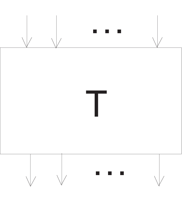
When $F$ is a rectangle with $n$ inputs at the top and $n$ outputs at the bottom. Let $H_{n}$ be the skein $\mathcal{S}(F)$ of $n$ -tangles. See Figure 3 for an element in $H_{n}$ .

Composing $n$ -tangles by placing one above another induces a product which makes $H_{n}$ into the Hecke algebra $H_{n}(z)$ with the coefficients ring $\Lambda$ , where $z=q-q^{-1}$ . $H_{n}(z)$ has a presentation generated by the elementary brads $\sigma_{i}$ subjects to the braid relations

(2.7)		$\displaystyle\sigma_{i}\sigma_{i+1}\sigma_{i}=\sigma_{i+1}\sigma_{i}\sigma_{i+1}$
	$\displaystyle\sigma_{i}\sigma_{j}=\sigma_{j}\sigma_{i},\|i-j\|\geq 1.$

and the quadratic relations $\sigma_{i}^{2}=z\sigma_{i}+1$ .

2.2.3. The annulus

When $F=S^{1}\times I$ is the annulus, we denote $\mathcal{C}=\mathcal{S}(S^{1}\times I)$ . $\mathcal{C}$ is a commutative algebra with the product induced by placing the annulus one outside other. For any element $T\in H_{n}$ , we use $\hat{T}$ to denote the closure of $T$ as showed in Figure 4.

It is clear that $\hat{T}\in\mathcal{C}$ . As an algebra, $\mathcal{C}$ is freely generated by the set $\{A_{m}:m\in\mathbb{Z}\}$ , $A_{m}$ for $m\neq 0$ is the closure of the braid $\sigma_{|m|-1}\cdots\sigma_{2}\sigma_{1}$ , and $A_{0}$ is the empty diagram [33]. It follows that $\mathcal{C}$ contains two subalgebras $\mathcal{C}_{+}$ and $\mathcal{C}_{-}$ which are generated by $\{A_{m}:m\in\mathbb{Z},m\geq 0\}$ and $\{A_{m}:m\in\mathbb{Z},m\leq 0\}$ . We denote the image of the closure map $H_{n}\rightarrow\mathcal{C}_{+}$ as $\mathcal{C}_{n}$ . Thus $\mathcal{C}_{+}=\cup_{n\geq 0}\mathcal{C}_{n}$ . The linear subspace $\mathcal{C}_{n}$ has a useful interpretation as the space of symmetric polynomials of degree $n$ in variables $x_{1},..,x_{N}$ , for large enough $N$ . $\mathcal{C}_{+}$ can be viewed as the algebra of the symmetric functions.

2.3. Basic elements in the skein of annulus $\mathcal{C}_{+}$

2.3.1. Turaev’s geometrical basis of $\mathcal{C}_{+}$

The element $A_{m}\in\mathcal{C}_{+}$ is the closure of the braid $\sigma_{m-1}\cdots\sigma_{2}\sigma_{1}\in H_{m}$ . Its mirror image $\bar{A}_{m}$ is the closure of the braid $\sigma_{m-1}^{-1}\cdots\sigma_{2}^{-1}\sigma_{1}^{-1}$ . Given a partition $\lambda=(\lambda_{1},..,\lambda_{l})$ of $m$ with length $l$ , we define the monomial $A_{\lambda}=A_{\lambda_{1}}\cdots A_{\lambda_{l}}$ . Then the monomials $\{A_{\lambda}\}_{\lambda\vdash m}$ becomes a basis of $\mathcal{C}_{m}$ which is called the Turaev’s geometric basis of $\mathcal{C}_{+}$ .

Moreover, let $A_{i,j}$ be the closure of the braid $\sigma_{i+j}\sigma_{i+j-1}\cdots\sigma_{j+1}\sigma_{j}^{-1}\cdots\sigma_{1}^{-1}$ . We define the element $X_{m}$ in $\mathcal{C}_{m}$ as $X_{m}=\sum_{i=0}^{m-1}A_{i,m-1-i}$ . There exist some explicit geometric relations between the elements $\bar{A}_{m}$ , $A_{m}$ and $X_{m}$ [26].

2.3.2. Symmetric function basis of $\mathcal{C}_{+}$

The subalgebra $\mathcal{C}_{+}\subset\mathcal{C}$ can be interpreted as the ring of symmetric functions in infinite variables $x_{1},..,x_{N},..$ [13]. The correspondence of the power sum symmetric function $p_{m}(x)$ in $\mathcal{C}_{m}$ is denoted by $P_{m}$ . Moreover, we have the identity

(2.8)

\displaystyle[m]P_{m}=zX_{m}.

Denoted by $Q_{\lambda}$ the closures of idempotent elements $e_{\lambda}$ in the Hecke algebra $H_{m}$ [1]. It was showed by Lukac [13] that $Q_{\lambda}$ represent the Schur functions in the interpretation as symmetric functions. Hence $\{Q_{\lambda}\}_{\lambda\vdash m}$ forms a basis of $\mathcal{C}_{m}$ . Furthermore, the Frobenius formula (2.2) gives

(2.9)

\displaystyle Q_{\lambda}=\sum_{\mu}\frac{\chi_{\lambda}(C_{\mu})}{z_{\mu}}P_{\mu},

where $P_{\mu}=\prod_{i=1}^{l(\mu)}P_{\mu_{i}}$ .

2.4. Notations

For brevity, the following notations will be used throughout the paper.

(2.10)

\displaystyle[d]=q^{d}-q^{-d},\ \Delta_{d}=\frac{q^{d}+q^{-d}}{2},\ \{d\}=\frac{[d]}{[1]}.

In particular, $[1]=z$ . For $\vec{\lambda}=(\lambda^{1},\lambda^{2},...,\lambda^{L}),\vec{\mu}=(\mu^{1},\mu^{2},...,\mu^{L})\in\mathcal{P}^{L}$ , we introduce

	$\displaystyle\\|\vec{\lambda}\\|$	$\displaystyle=\sum_{\alpha=1}^{L}\|\lambda^{\alpha}\|,\ \vec{\lambda}^{t}=((\lambda^{1})^{t},...,(\lambda^{L})^{t}),\ z_{\vec{\lambda}}=\prod_{\alpha=1}^{L}z_{\lambda^{\alpha}},\chi_{\vec{\lambda}}(\vec{\mu})=\prod_{\alpha=1}^{L}\chi_{\lambda^{\alpha}}(\mu^{\alpha}),$
	$\displaystyle Q_{\vec{\lambda}}$	$\displaystyle=\otimes_{\alpha=1}^{L}Q_{\lambda^{\alpha}},\ P_{\vec{\lambda}}=\otimes_{\alpha=1}^{L}P_{\lambda^{\alpha}},\ [\vec{\mu}]=\prod_{\alpha=1}^{L}\prod_{j=1}^{l(\mu^{\alpha})}[\mu_{j}^{\alpha}].$

2.5. Definitions of the colored HOMFLY-PT invariants

Let $\mathcal{L}$ be a framed link with $L$ components with a fixed numbering. For diagrams $Q_{1},..,Q_{L}$ in the skein model of annulus with the positive oriented core $\mathcal{C}_{+}$ , a link $\mathcal{L}$ decorated with $Q_{1},...,Q_{L}$ , denoted by $\mathcal{L}\star\otimes_{i=1}^{L}Q_{i}$ , is constructed by replacing every annulus $\mathcal{L}$ by the annulus with the diagram $Q_{i}$ such that the orientations of the cores match. Each $Q_{i}$ has a small backboard neighborhood in the annulus which makes the decorated link $\mathcal{L}\star\otimes_{i=1}^{L}Q_{i}$ into a framed link (see Figure 5 for a framed trefoil $\mathcal{K}$ decorated by skein element $\mathcal{Q}$ ).

In particular, when $Q_{\lambda^{\alpha}}\in\mathcal{C}_{d_{\alpha}}$ , where $\lambda^{\alpha}$ is the partition of a positive integer $d_{\alpha}$ , for $\alpha=1,..,L$ . The framed colored HOMFLY-PT invariant of $\mathcal{L}$ decorated by $Q_{\vec{\lambda}}$ is defined to be the framed HOMFLY-PT invariant of the decorated link $\mathcal{L}\star Q_{\vec{\lambda}}$ , i.e. $\mathcal{H}(\mathcal{L}\star Q_{\vec{\lambda}})$ . By adding a framing factor to eliminate the framing dependency

Definition 2.1.

The (framing-independence) colored HOMFLY-PT invariant is given by

(2.11)

\displaystyle W_{\vec{\lambda}}(\mathcal{L};q,t)=q^{-\sum_{\alpha=1}^{L}\kappa_{\lambda^{\alpha}}|w(\mathcal{K_{\alpha}})|}t^{-\sum_{\alpha=1}^{L}|\lambda^{\alpha}|w(\mathcal{K}_{\alpha})}\mathcal{H}(\mathcal{L}\star Q_{\vec{\lambda}}).

Some basic properties of the colored HOMFLY-PT invariant $W_{\vec{\lambda}}(\mathcal{L};q,t)$ are given in [15, 38]. For convenience, we also study the following reformulated colored HOMFLY-PT invariants.

Definition 2.2.

The reformulated colored HOMFLY-PT invariants are defined as:

(2.12)

\displaystyle\mathcal{Z}_{\vec{\mu}}(\mathcal{L};q,t)=\sum_{\vec{\lambda}}\chi_{\vec{\lambda}}(\vec{\mu})\mathcal{H}(\mathcal{L}\star Q_{\vec{\lambda}})=\mathcal{H}(\mathcal{L}\star P_{\vec{\mu}}),\ \check{\mathcal{Z}}_{\vec{\mu}}(\mathcal{L};q,t)=[\vec{\mu}]\mathcal{Z}_{\vec{\mu}}(\mathcal{L};q,t).

Remark 2.3.

From the view of the HOMFLY-PT skein theory, the reformulated colored HOMFLY-PT invariants $\mathcal{Z}_{\vec{\mu}}(\mathcal{L};q,t)$ or $\check{\mathcal{Z}}_{\vec{\mu}}(\mathcal{L};q,t)$ are simpler than the colored HOMFLY-PT invariant $W_{\vec{\lambda}}(\mathcal{L};q,t)$ , since the expression of $P_{\vec{\mu}}$ is simpler than $Q_{\vec{\lambda}}$ and has the nice property, see [26] for the similar statement. Therefore, it is natural to study the reformulated colored HOMFLY-PT invariant $\mathcal{Z}_{\vec{\mu}}(\mathcal{L};q,t)$ or $\check{\mathcal{Z}}_{\vec{\mu}}(\mathcal{L};q,t)$ instead of $W_{\vec{\lambda}}(\mathcal{L};q,t)$ .

3. Integrality property

We have introduced in Section 2, $P_{m}$ is the correspondence of the symmetric power function in the skein $\mathcal{C}_{+}$ . The geometric representation of $P_{m}$ is given by

(3.1)

\displaystyle[m]P_{m}=zX_{m}=z\sum_{i=0}^{m-1}A_{i,m-1-i},

where $A_{i,m-1-i}$ is the closure of the braid $\sigma_{m-1}\cdots\sigma_{m-i}\sigma_{m-i-1}^{-1}\cdots\sigma_{m-i-j}^{-1}$ . Let

(3.2)

\displaystyle\check{P}_{m}=[m]P_{m},\ \check{P}_{\mu}=\prod_{i=1}^{l(\mu)}\check{P}_{\mu_{i}}.

In particular, $P_{1}$ is the identity element in $\mathcal{C}_{+}$ . Thus $\check{\mathcal{Z}}_{((1),..,(1))}(\mathcal{L};q,t)=z^{L}\mathcal{H}(\mathcal{L};q,t)$ , for a link $\mathcal{L}$ with $L$ -components. For convenience, in the following, we will also use the notation $\check{\mathcal{Z}}(\mathcal{L};q,t)$ to denote $\check{\mathcal{Z}}_{((1),..,(1))}(\mathcal{L};q,t)$ and the notation $\check{\mathcal{Z}}_{p}(\mathcal{L};q,t)$ to denote $\check{\mathcal{Z}}_{((p),...,(p))}(\mathcal{L};q,t)$ . By the skein relation (2.4) of $\mathcal{H}(\mathcal{L})$ , we have

(3.3)

\displaystyle\check{\mathcal{Z}}(\mathcal{L}_{+};q,t)-\check{\mathcal{Z}}(\mathcal{L}_{-};q,t)=z^{2\epsilon}\check{\mathcal{Z}}(\mathcal{L}_{0};q,t).

where $\epsilon=0$ if the crossing is a self-crossing of a knot, $\epsilon=1$ if this crossing is a linking between two components of a link. Let $U$ be the unknot, we have $\check{\mathcal{Z}}(U;q,t)=t-t^{-1}$ . By using (3.3), it is obvious that

Lemma 3.1.

For any link $\mathcal{L}$ , $\check{\mathcal{Z}}(\mathcal{L};q,t)\in\mathbb{Z}[z^{2},t^{\pm 1}]$ .

Furthermore, we have

Theorem 3.2.

For any link $\mathcal{L}$ with $L$ components, and $\vec{\mu}=(\mu^{1},...,\mu^{L})\in\mathcal{P}^{L}$ ,

(3.4)

\displaystyle\check{\mathcal{Z}}_{\vec{\mu}}(\mathcal{L};q,t)\in\mathbb{Z}[z^{2},t^{\pm 1}].

Proof.

We first consider the knot case, for a knot $\mathcal{K}$ and a partition $\mu$ of length $l(\mu)=l$ . We will show that $\check{\mathcal{Z}}_{\mu}(\mathcal{K})\in\mathbb{Z}[z^{2},t^{\pm 1}]$ .

By the formula (3.2) and Lemma 3.1,

(3.5)

\displaystyle\check{\mathcal{Z}}_{(m)}(\mathcal{K})=\mathcal{H}(\mathcal{K}\star\check{P}_{m})=z\mathcal{H}(\mathcal{K}\star X_{m})=\check{\mathcal{Z}}(\mathcal{K}\star X_{m})\in\mathbb{Z}[z^{2},t^{\pm 1}]

We let $\mathcal{K}_{(l)}$ be the $l$ -cabling of the knot $\mathcal{K}$ which is a link of $l$ components. Then

(3.6)

\displaystyle\check{\mathcal{Z}}_{\mu}(\mathcal{K})=\mathcal{H}(\mathcal{K}\star\check{P}_{\mu})=z^{l}\mathcal{H}(\mathcal{K}_{(l)}\star\otimes_{j=1}^{l}X_{\mu_{j}})=\check{\mathcal{Z}}(\mathcal{K}_{(l)}\star\otimes_{j=1}^{l}X_{\mu_{j}})\in\mathbb{Z}[z^{2},t^{\pm 1}].

As to the case of the link $\mathcal{L}$ with $L$ components. Let $\vec{l}=(l^{1},...,l^{L})$ , where $l^{\alpha}=l(\mu^{\alpha})$ . We let $\mathcal{L}_{(\vec{l})}$ be the $\vec{l}$ -cabling of the link $\mathcal{L}$ which is a link of $\sum_{\alpha=1}^{L}l^{\alpha}$ components. Similarly, we have

(3.7)	$\displaystyle\check{\mathcal{Z}}_{\vec{\mu}}(\mathcal{L})$	$\displaystyle=\mathcal{H}(\mathcal{L}\star\check{P}_{\vec{\mu}})$
	$\displaystyle=z^{\sum_{\alpha=1}^{L}l^{\alpha}}\mathcal{H}(\mathcal{L}_{(\vec{l})}\star\otimes_{\alpha=1}^{L}\otimes_{j=1}^{l^{\alpha}}X_{\mu^{\alpha}_{j}})$
	$\displaystyle=\check{\mathcal{Z}}(\mathcal{L}_{(\vec{l})}\star\otimes_{\alpha=1}^{L}\otimes_{j=1}^{l^{\alpha}}X_{\mu^{\alpha}_{j}})\in\mathbb{Z}[z^{2},t^{\pm 1}].$

∎

4. Symmetries, Level-rank duality

In this section, we will prove the symmetries for colored HOMFLY-PT invariants as showed in the introduction.

Theorem 4.1.

Given a link $\mathcal{L}$ with $L$ components, and $\vec{\lambda}=(\lambda^{1},..,\lambda^{L})\in\mathcal{P}^{L}$ , we have the following symmetry:

(4.1)

\displaystyle W_{\vec{\lambda}}(\mathcal{L};q^{-1},t)=(-1)^{\|\vec{\lambda}\|}W_{\vec{\lambda}^{t}}(\mathcal{L};q,t)

Proof.

We only prove the case for a knot $\mathcal{K}$ , it is straightforward to generalize the proof to link case. For $\mu\in\mathcal{P}$ , by Theorem 3.2,

(4.2)

\displaystyle\check{\mathcal{Z}}_{\mu}(\mathcal{K};q,t)\in\mathbb{Z}[z^{2},t^{\pm 1}],

so $\check{\mathcal{Z}}_{\mu}(\mathcal{K};q^{-1},t)=\check{\mathcal{Z}}_{\mu}(\mathcal{K};q,t)$ . By $\check{\mathcal{Z}}_{\mu}(\mathcal{K};q,t)=[\mu]\mathcal{Z}_{\mu}(\mathcal{K};q,t)$ , we have

(4.3)

\displaystyle\mathcal{Z}_{\mu}(\mathcal{K};q^{-1},t)=(-1)^{l(\mu)}\mathcal{Z}_{\mu}(\mathcal{K};q,t).

Therefore,

(4.4)	$\displaystyle\mathcal{H}(\mathcal{K}\star Q_{\lambda};q^{-1},t)$	$\displaystyle=\sum_{\mu}\frac{\chi_{\lambda}(\mu)}{z_{\mu}}\mathcal{Z}_{\mu}(\mathcal{K};q^{-1},t)$
	$\displaystyle=\sum_{\mu}\frac{\chi_{\lambda}(\mu)}{z_{\mu}}(-1)^{l(\mu)}\mathcal{Z}_{\mu}(\mathcal{K};q,t)$
	$\displaystyle=(-1)^{\|\lambda\|}\sum_{\mu}\frac{\chi_{\lambda^{t}}(\mu)}{z_{\mu}}\mathcal{Z}_{\mu}(\mathcal{K};q,t)$
	$\displaystyle=(-1)^{\|\lambda\|}\mathcal{H}(\mathcal{K}\star Q_{\lambda^{t}};q,t)$

where we have used the fact

(4.5)

\displaystyle\chi_{\lambda^{t}}(\mu)=(-1)^{|\lambda|-l(\mu)}\chi_{\lambda}(\mu).

Moreover, since $\kappa_{\lambda}=-\kappa_{\lambda^{t}}$ and (2.11), finally, we get

(4.6)

\displaystyle W_{\lambda}(\mathcal{K};q^{-1},t)=(-1)^{|\lambda|}W_{\lambda^{t}}(\mathcal{K};q,t).

∎

Similarly, by Theorem 3.2, we also have

(4.7)

\displaystyle\mathcal{Z}_{\mu}(\mathcal{K};-q^{-1},t)=(-1)^{|\mu|+l(\mu)}\mathcal{Z}_{\mu}(\mathcal{K};q,t).

Thus, with the same procedure as in (4.4),

(4.8)

\displaystyle\mathcal{H}(\mathcal{K}\star Q_{\lambda};-q^{-1},t)=\mathcal{H}(\mathcal{K}\star Q_{\lambda^{t}};q,t).

Since $\kappa_{\lambda}$ is even and $\kappa_{\lambda}=-\kappa_{\lambda^{t}}$ , by (2.11), we have

Theorem 4.2.

Given a link $\mathcal{L}$ with $L$ components, and $\vec{\lambda}=(\lambda^{1},..,\lambda^{L})\in\mathcal{P}^{L}$ , then

(4.9)

\displaystyle W_{\vec{\lambda}}(\mathcal{L};-q^{-1},t)=W_{\vec{\lambda}^{t}}(\mathcal{L};q,t).

In order to show the third symmetry, for brevity, we introduce the function $OE$ to judge the parity of an integer $n\in\mathbb{Z}$ . In other words, $OE(n)=odd$ for $n$ odd, and $OE(n)=even$ for $n$ even. We also use the notation $L(\mathcal{L})$ to denote the number of the components of link $\mathcal{L}$ .

Lemma 4.3.

For a link $\mathcal{L}$ , all the degrees of $t$ in $\mathcal{H}(\mathcal{L};q,t)$ are odd if $OE(L(\mathcal{L})+w(\mathcal{L}))=odd$ or even if $OE(L(\mathcal{L})+w(\mathcal{L}))=even$ .

Proof.

By using the skein relation

(4.10)

\displaystyle\mathcal{H}(\mathcal{L}_{+})-\mathcal{H}(\mathcal{L}_{-})=(q-q^{-1})\mathcal{H}(\mathcal{L}_{0})

to resolve the crossings, and combing the Reidemeister moves of types II and III, any link $\mathcal{L}$ will eventually becomes a finite sum of the links $U^{\otimes k}\otimes T^{\otimes l}$ for some $k,l\in\mathbb{Z}_{+}$ , where $U$ and $T$ denote the unknot and a unknot with a positive kink respectively. We use the notation $S(\mathcal{L})$ to denote the set of all $U^{\otimes k}\otimes T^{\otimes l}$ that will appear in the final states after resolving all the crossings in $\mathcal{L}$ . In other words, for any link $\mathcal{L}$ , we always have the following expansion form:

(4.11)

\displaystyle\mathcal{H}(\mathcal{L})=\sum_{U^{\otimes k}\otimes T^{\otimes l}\in S(\mathcal{L})}a_{k,l}\mathcal{H}(U^{\otimes k}\otimes T^{\otimes l})

where all the coefficients $a_{k,l}$ are constants (only depends on $q$ ) independent of $t$ .

On the other hand side, it is easy to see the following identity always holds for any Conway triple $(\mathcal{L}_{+},\mathcal{L}_{-},\mathcal{L}_{0})$ :

(4.12)

\displaystyle OE(L(\mathcal{L}_{+})+w(\mathcal{L}_{+}))=OE(L(\mathcal{L}_{-})+w(\mathcal{L}_{-}))=OE(L(\mathcal{L}_{0})+w(\mathcal{L}_{0}))

Therefore, for all $U^{\otimes k}\otimes T^{\otimes l}\in S(\mathcal{L})$ , all the integers $L(U^{\otimes k}\otimes T^{\otimes l})+w(U^{\otimes k}\otimes T^{\otimes l})=k+2l$ have the same parity. It is clear that

(4.13)

\displaystyle\mathcal{H}(U^{\otimes k}\otimes T^{\otimes l})=\left(\frac{t-t^{-1}}{q-q^{-1}}\right)^{k+l}t^{l},

and the argument holds. Hence it also holds for $\mathcal{L}$ by formula (4.11). ∎

Next, we will prove the third symmetry.

Theorem 4.4.

Given a link $\mathcal{L}$ with $L$ components, and $\vec{\lambda}=(\lambda^{1},..,\lambda^{L})\in\mathcal{P}^{L}$ , we have

(4.14)

\displaystyle W_{\vec{\lambda}}(\mathcal{L};q,-t)=(-1)^{\|\vec{\lambda}\|}W_{\vec{\lambda}}(\mathcal{L};q,t).

Proof.

We only prove the case for a knot $\mathcal{K}$ , it is straightforward to write the proof for link case. By the formula (3.1) for $P_{m}$ , we have

(4.15)

\displaystyle P_{m}=\frac{1}{\{m\}}\left(\sum_{i=0}^{m-1}\widehat{\sigma_{m-1}\sigma_{m-2}\cdots\sigma_{m-1-i}^{-1}\cdots\sigma_{2}^{-1}\sigma_{1}^{-1}}\right).

For a general term $\widehat{\sigma_{m-1}\sigma_{m-2}\cdots\sigma_{m-1-i}^{-1}\cdots\sigma_{2}^{-1}\sigma_{1}^{-1}}$ , the writhe number is given by

(4.16)

\displaystyle w(\widehat{\sigma_{m-1}\cdots\sigma_{m-1-i}^{-1}\cdots\sigma_{1}^{-1}})=2i-(m-1).

So for a knot $\mathcal{K}$ ,

(4.17)

\displaystyle w(\mathcal{K}\star\widehat{\sigma_{m-1}\cdots\sigma_{m-1-i}^{-1}\cdots\sigma_{1}^{-1}})=mw(\mathcal{K})+2i-(m-1).

and the number of components is

(4.18)

\displaystyle L(\mathcal{K}\star\widehat{\sigma_{m-1}\cdots\sigma_{m-1-i}^{-1}\cdots\sigma_{1}^{-1}})=1.

Therefore,

(4.19)			$\displaystyle L(\mathcal{K}\star\widehat{\sigma_{m-1}\cdots\sigma_{m-1-i}^{-1}\cdots\sigma_{1}^{-1}})+w(\mathcal{K}\star\widehat{\sigma_{m-1}\cdots\sigma_{m-1-i}^{-1}\cdots\sigma_{1}^{-1}})$
		$\displaystyle=m(w(\mathcal{K})-1)+2(i+1).$

By Lemma 4.3, we have

(4.20)			$\displaystyle\mathcal{H}(\mathcal{K}\star\widehat{\sigma_{m-1}\cdots\sigma_{m-1-i}^{-1}\cdots\sigma_{1}^{-1}};q,-t)$
		$\displaystyle=(-1)^{m(w(\mathcal{K})-1)}\mathcal{H}(\mathcal{K}\star\widehat{\sigma_{m-1}\cdots\sigma_{m-1-i}^{-1}\cdots\sigma_{1}^{-1}};q,t)$

Hence,

(4.21)

\displaystyle\mathcal{Z}_{m}(\mathcal{K};q,-t)=(-1)^{m(w(\mathcal{K})-1)}\mathcal{Z}_{m}(\mathcal{K};q,t).

More general, for a partition $\mu$ , one also has

(4.22)

\displaystyle\mathcal{Z}_{\mu}(\mathcal{K};q,-t)=(-1)^{|\mu|(w(\mathcal{K})-1)}\mathcal{Z}_{\mu}(\mathcal{K};q,t).

Thus,

(4.23)

\displaystyle\mathcal{H}(\mathcal{K}\star Q_{\lambda},q,-t)=(-1)^{|\lambda|(w(\mathcal{K})-1)}\mathcal{H}(\mathcal{K}\star Q_{\lambda},q,t)

Therefore,

(4.24)		$\displaystyle W_{\lambda}(\mathcal{K};q,-t)$	$\displaystyle=q^{-\kappa_{\lambda}w(\mathcal{K})}t^{-\|\lambda\|w(\mathcal{K})}(-1)^{-\|\lambda\|w(\mathcal{K})}\mathcal{H}(\mathcal{K}\star Q_{\lambda},q,-t)$
		$\displaystyle=(-1)^{\|\lambda\|}W_{\lambda}(\mathcal{K};q,t)$

∎

Combing the above two identities in Theorem 4.1 and Theorem 4.4, we obtain the following rank-level duality as showed in [21, 16]:

Corollary 4.5.

Given a link $\mathcal{L}$ with $L$ components, and $\vec{\lambda}=(\lambda^{1},..,\lambda^{L})\in\mathcal{P}^{L}$ ,

(4.25)

\displaystyle W_{\vec{\lambda}^{t}}(\mathcal{L};q^{-1},-t)=W_{\vec{\lambda}}(\mathcal{L};q,t).

5. More results on reformulated colored HOMFLY-PT invariants

In this section, we will provide more basic results of the reformulated colored HOMFLY-PT invariants. These formulas are very useful in proof of the LMOV conjecture [15, 17] which motivates us to study the congruent skein relations.

5.1. Framing change formula

Let $\mathcal{C}_{+}$ be the HOMFLY-PT skein of annulus with positive orientation. We have showed that $\{Q_{\lambda}\}$ forms a basis of this skein. We define the framing map $\mathfrak{f}^{\tau}:\mathcal{C}_{+}\rightarrow\mathcal{C}_{+}$ as the linear map defined on the basis $\{Q_{\lambda}\}$ by

(5.1)

\displaystyle\mathfrak{f}^{\tau}(Q_{\lambda})=q^{\kappa_{\lambda}\tau}t^{|\lambda|\tau}Q_{\lambda}.

For $\vec{\tau}=(\tau^{1},..,\tau^{L})$ ,

(5.2)

\displaystyle\mathfrak{f}^{\vec{\tau}}(Q_{\vec{\lambda}})=\otimes_{\alpha=1}^{L}\mathfrak{f}^{\tau^{\alpha}}(Q_{\lambda^{\alpha}}).

We define the reformulated colored HOMFLY-PT invariant $\mathcal{Z}_{\vec{\mu}}(\mathcal{L};q,t;\vec{\tau})$ with framing $\vec{\tau}$ as follow

(5.3)

\displaystyle\mathcal{Z}_{\vec{\mu}}(\mathcal{L};q,t;\vec{\tau})=\mathcal{H}(\mathcal{L}\star\mathfrak{f}^{\vec{\tau}}(P_{\vec{\mu}})).

Lemma 5.1.

Given $\mu,\nu\in\mathcal{P}_{+}$ , we define the following function

(5.4)

\displaystyle\phi_{\mu,\nu}(x)=\sum_{\lambda}\chi_{\lambda}(\mu)\chi_{\lambda}(\nu)x^{\kappa_{\lambda}},

then we have $\phi_{(d),\mu}=[d\mu]_{x}/[d]_{x}$ .

Proof.

If $\lambda$ is a hook partition $(a+1,1,1,...,1)$ , then $\kappa_{\lambda}=(a+1)a-(b+1)b$ , where $b+1$ is the length of the partition and we may also write it as $(a|b)$ . Note that

(5.5a)		$\displaystyle\chi_{\lambda}((d))=$	$\displaystyle(-1)^{b},$	if $\lambda$ is a hook partition $(a\|b)$ ,
	$\displaystyle\chi_{\lambda}((d))=$	$\displaystyle 0,$	otherwise;

and $\kappa_{(a|b)}=(a-b)d$ . By problem $14$ at page $49$ of [23], taking $t=y$ , we have

(5.6)

\displaystyle\prod_{i}\frac{1-y^{-1}x_{i}}{1-yx_{i}}=E(-y^{-1})H(y)=1+(y-y^{-1})\sum_{\mu}\frac{p_{\mu}(x)}{z_{\mu}}\sum_{a,b\geq 0}\chi_{(a|b)}(\mu)(-1)^{b}y^{a-b}.

since $s_{(a|b)}(x)=\sum_{\mu}\frac{\chi_{(a|b)}(mu)}{z_{\mu}}p_{\mu}(x)$ . On the other hand,

(5.7)	$\displaystyle E(-y^{-1})H(y)$	$\displaystyle=\frac{H(y)}{H(y^{-1})}$
	$\displaystyle=\exp\left(\sum_{r\geq 1}\frac{p_{r}(x)}{r}(y^{r}-y^{-r})\right)$
	$\displaystyle=\prod_{r\geq 1}\exp\left(\frac{p_{r}(x)}{r}(y^{r}-y^{-r})\right)$
	$\displaystyle=\prod_{r\geq 1}\sum_{m_{r}\geq 0}\frac{p_{r}(x)^{m_{r}}(y^{r}-y^{-r})^{m_{r}}}{r^{m_{r}}m_{r}!}$
	$\displaystyle=\sum_{\mu}\frac{p_{\mu}(x)}{z_{\mu}}\prod_{j=1}^{l(\mu)}(y^{\mu_{j}}-y^{-\mu_{j}})$

Comparing the coefficients of $p_{\mu}(x)$ in (5.6), we obtain

(5.8)

\displaystyle\sum_{a+b+1=|\mu|}\chi_{(a|b)}(\mu)(-1)^{b}y^{a-b}=\frac{\prod_{j=1}^{l(\mu)}(y^{\mu_{j}}-y^{-\mu_{j}})}{y-y^{-1}}

Letting $y=x^{d}$ , we complete the proof. ∎

The definition of framing map implies

(5.9)	$\displaystyle\mathfrak{f}^{\tau}(P_{d})$	$\displaystyle=\sum_{\|\lambda\|=d}\chi_{\lambda}((d))\mathfrak{f}^{\tau}_{\lambda}\cdot Q_{\lambda}$
	$\displaystyle=\sum_{\|\lambda\|=d}\chi_{\lambda}((d))q^{\kappa_{\lambda}\tau}t^{d\tau}\sum_{\|\mu\|=d}\frac{\chi_{\lambda}(\mu)}{z_{\mu}}P_{\mu}$
	$\displaystyle=t^{d\tau}\sum_{\|\mu\|=d}\frac{P_{\mu}}{z_{\mu}}\phi_{(d),\mu}(q^{\tau}).$

Therefore, by Lemma 5.1, we obtain

Theorem 5.2 (Framing change formula).

Given any framing $\tau$ , we have

(5.10)

\displaystyle\mathcal{Z}_{(d)}(\mathcal{K};\tau)=t^{d\tau}\sum_{|\mu|=d}\frac{\mathcal{Z}_{\mu}(\mathcal{K})}{z_{\mu}}\frac{[d\tau\mu]}{[d\tau]},

for given $\tau_{0}$ and $\tau$ , we have

(5.11)

\displaystyle\mathcal{Z}_{(d)}(\mathcal{K};\tau_{0}+\tau)=t^{d\tau}\sum_{|\mu|=d}\frac{\mathcal{Z}_{\mu}(\mathcal{K};\tau_{0})}{z_{\mu}}\frac{[d\tau\mu]}{[d\tau]}.

As to link case, we also have

Corollary 5.3.

For given $\vec{\tau},\vec{\tau}_{0}$ and $\vec{d}=((d_{1}),...,(d_{L}))$ , we have

(5.12)

\displaystyle\mathcal{Z}_{\vec{d}}(\mathcal{L};\vec{\tau}_{0}+\vec{\tau})=t^{\sum_{\alpha=1}^{L}d_{\alpha}\tau^{\alpha}}\sum_{|\mu^{\alpha}|=d_{\alpha}}\frac{\mathcal{Z}_{\vec{\mu}}(\mathcal{L};\vec{\tau}_{0})}{z_{\vec{\mu}}}\cdot\prod_{\alpha=1}^{L}\frac{[d_{\alpha}\tau^{\alpha}\mu^{\alpha}]}{[d_{\alpha}\tau^{\alpha}]}.

5.2. Congruent framing change formula

By simple computations, we have the following result:

Lemma 5.4.

If $m$ is even, then $q^{md}+q^{-md}\in\mathbb{Z}[[d]^{2}]$ ; if $m$ is odd, we have

(5.13)

\displaystyle q^{md}+q^{-md}\in(q^{d}+q^{-d})+(q^{d}+q^{-d})[d]^{2}\cdot\mathbb{Z}[[d]^{2}].

Example 5.5.

Let $k\in\mathbb{Z}$ , we have

(5.14)			$\displaystyle q^{2k}+q^{-2k}\in\mathbb{Z}[[1]^{2}],\ q^{2k+1}+q^{-(2k+1)}\in(q+q^{-1})+(q+q^{-1})[1]^{2}\cdot\mathbb{Z}[[1]^{2}]$
(5.15)			$\displaystyle q^{2k+1}-q^{-(2k+1)}=[1]\cdot\left(\sum_{i=1}^{k}(q^{2i}+q^{-2i})+1\right)\in[1]\mathbb{Z}[[1]^{2}],$
(5.16)			$\displaystyle[d]^{2}=(q^{d}-q^{-d})^{2}=q^{2d}+q^{-2d}-2\in\mathbb{Z}[[1]^{2}],$
(5.17)			$\displaystyle\frac{q^{2k+1}\pm q^{-(2k+1)}}{q\pm q^{-1}}\in\mathbb{Z}[[1]^{2}],$
(5.18)			$\displaystyle\left(\frac{q^{d}-q^{-d}}{q-q^{-1}}\right)^{2k}\in\mathbb{Z}[[1]^{2}].$

Definition 5.6.

Let $f(q,t),g(q,t)\in\mathbb{Z}[q^{\pm 1},t^{\pm 1}]$ , if there exists a function $h(z)\in\mathbb{Q}[z^{2}]$ , where $z=q-q^{-1}$ , such that $f(q,t)-g(q,t)=\{d\}^{2}\cdot h(z)$ . Then we define

(5.19)

\displaystyle f(q,t)\equiv g(q,t)\mod\{d\}^{2}.

Lemma 5.7.

Let $m$ and $d$ are two integers, we have

(5.20)		$\displaystyle\Delta_{dm}$	$\displaystyle\equiv\Delta_{d}^{m}\mod\{d\}^{2},\ \text{when}\ m=2k\ \text{or}\ m=1,$
(5.21)		$\displaystyle\frac{[md]}{[d]}$	$\displaystyle\equiv m\Delta_{d}^{m-1}\mod\{d\}^{2},\ \text{when}\ m=2k+1\ \text{or}\ m=2.$

Proof.

It is clear when $m=1$ , $m=2$ , the Lemma 5.7 holds. By Lemma 5.4, when $m=2k$ , $\Delta_{dm}=\frac{q^{2kd}+q^{-2kd}}{2}=c_{1}[d]^{2k}+c_{2}[d]^{2(k-1)}+\cdots+1,$ and $\Delta_{d}^{2k}=\left(\frac{q^{d}+q^{-d}}{2}\right)^{2k}=c^{\prime}_{1}[d]^{2k}+c^{\prime}_{2}[d]^{2k-2}+\cdots+1.$ Thus $\Delta_{2kd}-\Delta_{d}^{2k}\in[d]^{2}\cdot\mathbb{Q}[[d]^{2}]=[d]^{2}\cdot\mathbb{Q}[z^{2}].$

Similarly, when $m=2k+1$ ,

(5.22)	$\displaystyle\frac{[(2k+1)d]}{[d]}$	$\displaystyle=\frac{q^{(2k+1)d}-q^{-(2k+1)d}}{q^{d}-q^{-d}}$
	$\displaystyle=q^{2kd}+q^{(2k-2)d}+\cdots+1+\cdots+q^{-(2k-2)d}+q^{-2kd}$
	$\displaystyle=c_{1}[d]^{2k}+\cdots+(2k+1).$

and $(2k+1)\Delta_{d}^{2k}=c^{\prime}_{1}[d]^{2k}+\cdots+(2k+1)$ . Thus $\frac{[(2k+1)d]}{[d]}-(2k+1)\Delta_{d}^{2k}\in[d]^{2}\cdot\mathbb{Q}[[d]^{2}]=[d]^{2}\cdot\mathbb{Q}[z^{2}].$ ∎

Lemma 5.8.

Let $p$ be a prime number, we have

(5.23)

\displaystyle\triangle_{p}^{p-1}\equiv(-1)^{p-1}\mod\{p\}^{2}.

Proof.

By definition, it is easy to see

(5.24)

\displaystyle\Delta_{p}^{2k}=\left(\frac{q^{p}+q^{-p}}{2}\right)^{2k}=1+c_{1}[p]^{2}+\cdots c_{2k-2}[p]^{2k-2}+c_{2k}[p]^{2k}.

So when $p$ is an odd prime, then $\triangle_{p}^{p-1}\equiv 1\mod\{p\}^{2}.$

When $p=2$ , we have

(5.25)

\displaystyle\triangle_{p}^{p-1}=\triangle_{2}^{1}=\frac{q^{2}+q^{-2}}{2}=\frac{(q+q^{-1})^{2}}{2}-1\equiv-1\mod\{2\}^{2}.

∎

By Lemma 5.7, we have for any prime number $p$ ,

(5.26)

\displaystyle\frac{[p^{2}]}{p[p]}\equiv\Delta_{p}^{p-1}\mod\{p\}^{2}.

Furthermore, if $p$ is a prime number, $p$ is coprime to any $\mu_{i}$ , $i=1,2,...,l(\mu)$ , for $|\mu|=p$ and $l(\mu)\geq 2$ , a direct counting of the unit roots gives the following structure

(5.27)

\displaystyle\frac{[p\mu]}{[\mu]}\in\{p\}^{2}\cdot\mathbb{Z}[z^{2}].

On the other hand side, the formula (5.9) shows

(5.28)

\displaystyle\mathfrak{f}^{1+\tau}(\check{P}_{d})=t^{d}\left(\mathfrak{f}^{\tau}(\check{P}_{d})\frac{[d^{2}]}{d[d]}+\sum_{|\mu|=d}\frac{\mathfrak{f}^{\tau}(\check{P}_{\mu})}{z_{\mu}}\frac{[d\mu]}{[\mu]}\right).

So combing the Lemma 5.7 and 5.8, we obtain the following results:

Theorem 5.9.

Given a knot $\mathcal{K}$ and a framing $\tau$ , if $p$ is a prime number, then

(5.29)

\displaystyle\check{\mathcal{Z}}_{p}(\mathcal{K};\tau)\equiv t^{p\tau}(-1)^{\tau(p-1)}\check{\mathcal{Z}}_{p}(\mathcal{K})\mod\{p\}^{2}.

We use the notation $\mathcal{L}^{+1}$ to denote the link obtained by adding a positive kink to the $\alpha$ -th component of link $\mathcal{L}$ , then

(5.30)

\displaystyle\check{\mathcal{Z}}_{p}(\mathcal{L}^{+1})=\check{\mathcal{Z}}_{p}(\mathcal{L};\vec{\tau}=(0,..,\tau^{\alpha}=1,0..,0)).

Therefore, we have

Theorem 5.10.

When $p$ is prime,

(5.31)

\displaystyle\check{\mathcal{Z}}_{p}(\mathcal{\mathcal{L}}^{+1})\equiv(-1)^{p-1}t^{p}\check{\mathcal{Z}}_{p}(\mathcal{\mathcal{L}})\mod\{p\}^{2}.

6. Congruent skein relations for (reformulated) colored HOMFLY-PT invariants

We have showed in Section 3, the reformulated colored HOMFLY-PT invariant $\check{\mathcal{Z}}_{p}(\mathcal{L};q,t)$ has nice properties. $\check{\mathcal{Z}}_{p}(\mathcal{L};q,t)$ can be viewed as the generalization of the classical HOMFLY-PT polynomial $\mathcal{H}(\mathcal{L};q,t)$ . By this definition, for a link $\mathcal{L}$ with $L$ -components, $\check{\mathcal{Z}}_{1}(\mathcal{L};q,t)$ is equal to the classical (framing dependence) HOMFLY-PT polynomial $\mathcal{H}(\mathcal{L};q,t)$ by multiplying a factor $z^{L}$ , i.e $\check{\mathcal{Z}}_{1}(\mathcal{L};q,t)=z^{L}\mathcal{H}(\mathcal{L};q,t)$ . The skein relation for $\mathcal{H}(\mathcal{L};q,t)$ leads to the skein relation for $\check{\mathcal{Z}}_{1}(\mathcal{L};q,t)$ as follow:

\check{\mathcal{Z}}_{1}(\mathcal{L}_{+};q,t)-\check{\mathcal{Z}}_{1}(\mathcal{L}_{-};q,t)=\check{\mathcal{Z}}_{1}(\mathcal{L}_{0};q,t),

when the crossing is the self-crossing of a component of the link $\mathcal{L}$ , and

\check{\mathcal{Z}}_{1}(\mathcal{L}_{+};q,t)-\check{\mathcal{Z}}_{1}(\mathcal{L}_{-};q,t)=z^{2}\check{\mathcal{Z}}_{1}(\mathcal{L}_{0};q,t),

when the crossing is the linking of two different components of the link $\mathcal{L}$ .

We expect $\check{\mathcal{Z}}_{p}$ has the similar behavior with $\check{\mathcal{Z}}_{1}$ . So it is natural to ask if there exist the skein relation for $\check{\mathcal{Z}}_{p}$ ? Based on the new approach to LMOV conjecture [17], we propose the following congruent skein relations for the reformulated colored HOMFLY-PT invariants $\check{\mathcal{Z}}_{p}$ .

Conjecture 6.1 (Congruent skein relations).

For any link $\mathcal{L}$ and a prime number $p$ , we have

(6.1)

\displaystyle\check{\mathcal{Z}}_{p}(\mathcal{L}_{+})-\check{\mathcal{Z}}_{p}(\mathcal{L}_{-})\equiv(-1)^{p-1}\check{\mathcal{Z}}_{p}(\mathcal{L}_{0})\mod\{p\}^{2},

when the crossing is the self-crossing of a knot, and

(6.2)

\displaystyle\check{\mathcal{Z}}_{p}(\mathcal{L}_{+})-\check{\mathcal{Z}}_{p}(\mathcal{L}_{-})\equiv(-1)^{p-1}p[p]^{2}\check{\mathcal{Z}}_{p}(\mathcal{L}_{0})\mod\{p\}^{2}[p]^{2}.

when the crossing is the linking of two different components of the link $\mathcal{L}$ . Where the notation $A\equiv B\mod C$ denotes $\frac{A-B}{C}\in\mathbb{Z}[(q-q^{-1})^{2},t^{\pm 1}].$

6.1. Confirmations

The congruent skein relations (6.1) and (6.2) in Conjecture 6.1 have been tested by a lot of examples (see Appendix 8 for some sample examples). In the following, we show some partial results for Conjecture 6.1.

Theorem 6.2.

Proof.

According to the Theorem 5.9, we have

(6.3)		$\displaystyle\check{\mathcal{Z}}_{p}(\mathcal{K}_{+})$	$\displaystyle=\check{\mathcal{Z}}_{p}(\mathcal{K};\tau=1)\equiv t^{p}(-1)^{p-1}\check{\mathcal{Z}}_{p}(\mathcal{K})\mod\{p\}^{2},$
	$\displaystyle\check{\mathcal{Z}}_{p}(\mathcal{K}_{-})$	$\displaystyle=\check{\mathcal{Z}}_{p}(\mathcal{K};\tau=-1)\equiv t^{-p}(-1)^{p-1}\check{\mathcal{Z}}_{p}(\mathcal{K})\mod\{p\}^{2}.$

Therefore,

(6.4)

\displaystyle\check{\mathcal{Z}}_{p}(\mathcal{K}_{+})-\check{\mathcal{Z}}_{p}(\mathcal{K}_{-})\equiv(-1)^{p-1}\check{\mathcal{Z}}_{p}(\mathcal{K}\otimes U)\mod\{p\}^{2}.

since $\check{\mathcal{Z}}_{p}(U)=t^{p}-t^{-p}$ . ∎

Theorem 6.3.

For the Conway triple $\mathcal{L}_{+}=4_{1}$ , $\mathcal{L}_{-}$ = unknot with two negative kinks and $\mathcal{L}_{0}=T(2,-2)$ with one positive kink. The congruent skein relation (6.1) holds for $p=2,3$ .

Proof.

See examples 8.1 and 8.2 in Appendix 8. ∎

Theorem 6.4.

Let $k\in\mathbb{Z}$ , for the triple $\mathcal{L}_{+}=T(2,2k+1)$ , $\mathcal{L}_{-}=T(2,2k-1)$ , $\mathcal{L}_{0}=T(2,2k)$ , the congruent skein relation (6.1) holds for $p=2$ .

Similarly, for the triple $\mathcal{L}_{+}=T(2,2k)$ , $\mathcal{L}_{-}=T(2,2k-2)$ , $\mathcal{L}_{0}=T(2,2k-1)$ , the congruent skein relation (6.2) holds for $p=2$ .

Proof.

In fact, we need to prove the following two formulas:

(6.5)

\displaystyle\check{\mathcal{Z}}_{(2)}(T(2,2k+1))-\check{\mathcal{Z}}_{(2)}(T(2,2k-1))+\check{\mathcal{Z}}_{(2)(2)}(T(2,2k))\equiv 0\mod\{2\}^{2}.

(6.6)			$\displaystyle\check{\mathcal{Z}}_{(2)(2)}(T(2,2k))-\check{\mathcal{Z}}_{(2)(2)}(T(2,2k-2))$
		$\displaystyle+2[2]^{2}\check{\mathcal{Z}}_{(2)}(T(2,2k-1))\equiv 0\mod\{2\}^{2}[2]^{2}.$

Given a partition $\lambda$ , we define $s_{\lambda}=\sum_{\mu}\frac{\chi_{\lambda}(\mu)}{z_{\mu}}\prod_{i=1}^{l(\mu)}\frac{t^{\mu_{i}}-t^{-\mu_{i}}}{q^{\mu_{i}}-q^{-\mu_{i}}}.$ By formula (5.21) in the paper of [22], we have

	$\displaystyle W_{(2)(2)}(T(2,2k))$	$\displaystyle=q^{8k}s_{(4)}+s_{(3,1)}+q^{-4k}s_{(2,2)},$
	$\displaystyle W_{(2)(1,1)}(T(2,2k))$	$\displaystyle=q^{4k}s_{(3,1)}+q^{-4k}s_{(2,1,1)},$
	$\displaystyle W_{(1,1)(1,1)}(T(2,2k))$	$\displaystyle=q^{4k}s_{(4)}+s_{(2,1,1)}+q^{-8k}s_{(1,1,1,1)},$
	$\displaystyle W_{(2)}(T(2,2k+1))$	$\displaystyle=q^{4k+2}(q^{4k+2}s_{(4)}-q^{-(4k+2)}s_{(3,1)}+q^{-(8k+4)}s_{(2,2)}),$
	$\displaystyle W_{(1,1)}(T(2,2k+1))$	$\displaystyle=q^{-(4k+2)}(q^{8k+4}s_{(2,2)}-q^{4k+2}s_{(2,1,1)}+q^{-(4k+2)}s_{(1,1,1,1)}).$

Therefore, we obtain

$\check{\mathcal{Z}}_{(2)(2)}(T(2,2k))=[2]^{2}\mathcal{Z}_{(2)(2)}(T(2,2k))$

$=[2]^{2}(W_{(2)(2)}(T(2,2k))-2W_{(2)(1,1)}(T(2,2k))+W_{(1,1)(1,1)}(T(2,2k)))$

$=[2]^{2}(q^{8k}s_{(4)}+(1-2q^{4k})s_{(3,1)}+(q^{4k}+q^{-4k})s_{(2,2)}+(1-2q^{-4k})s_{(2,1,1)}+q^{-8k}s_{(1,1,1,1)})$

$=\frac{1}{4}(q^{4k}+2+q^{-4k})(q^{4k}-q^{-4k})\frac{t^{4}-t^{-4}}{q^{4}-q^{-4}}(q^{2}-q^{-2})^{2}$

$+\frac{1}{3}(q^{6k}-q^{-6k})(q^{2k}-q^{-2k})\frac{t^{3}-t^{-3}}{q^{3}-q^{-3}}\frac{t-t^{-1}}{q-q^{-1}}(q^{2}-q^{-2})^{2}$

$+\frac{1}{8}(q^{8k}+4q^{4k}-2+4q^{-4k}+q^{-8k})(t^{2}-t^{-2})^{2}$

$+\frac{1}{4}[(q^{8k}-q^{-8k})-2(q^{4k}-q^{-4k})](t^{2}-t^{-2})(t-t^{-1})^{2}\frac{(q+q^{-1})^{2}}{q^{2}-q^{-2}}$

$+\frac{1}{24}(q^{2k}-q^{-2k})^{4}\left(\frac{t-t^{-1}}{q-q^{-1}}\right)^{4}(q^{2}-q^{-2})^{2}$

$=\frac{1}{4}(q^{2k}+q^{-2k})^{2}\frac{q^{4k}-q^{-4k}}{q^{4}-q^{-4}}(t^{4}-t^{-4})(q^{2}-q^{-2})^{2}$

$+\frac{1}{3}\frac{q^{6k}-q^{-6k}}{q^{6}-q^{-6}}\frac{q^{2k}-q^{-2k}}{q^{2}-q^{-2}}(q^{3}+q^{-3})(q+q^{-1})(t^{3}-t^{-3})(t-t^{-1})(q^{2}-q^{-2})^{2}$

$+\frac{1}{8}(q^{8k}+4q^{4k}-2+4q^{-4k}+q^{-8k})(t^{2}-t^{-2})^{2}$

$+\frac{1}{4}\left(\frac{q^{2k}-q^{-2k}}{q^{2}-q^{-2}}\right)^{2}\frac{q^{4k}-q^{-4k}}{q^{4}-q^{-4}}(q^{2}+q^{-2})(t^{2}-t^{-2})(t-t^{-1})^{2}(q+q^{-1})^{2}(q^{2}-q^{-2})^{2}$

$+\frac{1}{24}\left(\frac{q^{2k}-q^{-2k}}{q^{2}-q^{-2}}\right)^{4}(q+q^{-1})^{4}\left(t-t^{-1}\right)^{4}(q^{2}-q^{-2})^{2}$

Obviously, $\frac{q^{6k}-q^{-6k}}{q^{6}-q^{-6}}$ , $\frac{q^{4k}-q^{-4k}}{q^{4}-q^{-4}}$ , $\frac{q^{2k}-q^{-2k}}{q^{2}-q^{-2}}$ are polynomials of $q-q^{-1}$ .

Moreover

$(q^{3}+q^{-3})(q+q^{-1})\equiv(q+q^{-1})^{2}(q^{2}-q^{-2})^{2}$

$\equiv(q+q^{-1})^{4}\left(t-t^{-1}\right)^{4}(q^{2}-q^{-2})^{2}\equiv 0\mod\{2\}^{2}[2]^{2}$ .

So we get

$\check{\mathcal{Z}}_{(2)(2)}(T(2,2k))\equiv\frac{1}{4}(q^{2k}+q^{-2k})^{2}\frac{q^{4k}-q^{-4k}}{q^{4}-q^{-4}}(t^{4}-t^{-4})(q^{2}-q^{-2})^{2}$

$+\frac{1}{8}(q^{8k}+4q^{4k}-2+4q^{-4k}+q^{-8k})(t^{2}-t^{-2})^{2}\mod\{2\}^{2}[2]^{2}$

$=\frac{1}{4}(q^{2k}+q^{-2k})^{2}\frac{q^{4k}-q^{-4k}}{q^{4}-q^{-4}}(t^{4}-t^{-4})(q^{2}-q^{-2})^{2}$

$+\frac{1}{8}(q^{8k}-4q^{4k}+6-4q^{-4k}+q^{-8k}+8q^{4k}-16+8q^{-4k}+8)(t^{2}-t^{-2})^{2}\mod\{2\}^{2}[2]^{2}$

$=\frac{1}{4}(q^{2k}+q^{-2k})^{2}\frac{q^{4k}-q^{-4k}}{q^{4}-q^{-4}}(t^{4}-t^{-4})(q^{2}-q^{-2})^{2}$

$+\frac{1}{8}(q^{2k}-q^{-2k})^{4}(t^{2}-t^{-2})^{2}+(q^{2k}-q^{-2k})^{2}(t^{2}-t^{-2})^{2}+(t^{2}-t^{-2})^{2}\mod\{2\}^{2}[2]^{2}$

$=\frac{1}{4}(q^{2k}+q^{-2k})^{2}\frac{q^{4k}-q^{-4k}}{q^{4}-q^{-4}}(t^{4}-t^{-4})(q^{2}-q^{-2})^{2}$

$+\frac{1}{8}\left(\frac{q^{2k}-q^{-2k}}{q^{2}-q^{-2}}\right)^{4}(t^{2}-t^{-2})^{2}(q^{2}-q^{-2})^{4}$

$+\left(\frac{q^{2k}-q^{-2k}}{q^{2}-q^{-2}}\right)^{2}(t^{2}-t^{-2})^{2}(q^{2}-q^{-2})^{2}+(t^{2}-t^{-2})^{2}\mod\{2\}^{2}[2]^{2}$

$\equiv\frac{1}{4}(q^{2k}+q^{-2k})^{2}\frac{q^{4k}-q^{-4k}}{q^{4}-q^{-4}}(t^{4}-t^{-4})(q^{2}-q^{-2})^{2}$

$+\left(\frac{q^{2k}-q^{-2k}}{q^{2}-q^{-2}}\right)^{2}(t^{2}-t^{-2})^{2}(q^{2}-q^{-2})^{2}+(t^{2}-t^{-2})^{2}\mod\{2\}^{2}[2]^{2}$

We also have

(6.7)

\displaystyle\check{\mathcal{Z}}_{(2)(2)}(T(2,2k))\equiv(t^{2}-t^{-2})^{2}\mod[2]^{2}

Moreover, with the similar analysis, we have

(6.8)			$\displaystyle\check{\mathcal{Z}}_{(2)}(T(2,2k+1))\equiv\left(\frac{1}{4}(q^{4k+2}+q^{-(4k+2)})^{2}\frac{t^{4}-t^{-4}}{q^{4}-q^{-4}}\right.$
		$\displaystyle\left.+\frac{1}{8}(q^{4k+2}-q^{-(4k+2)})(q^{2k+1}-q^{-(2k+1)})^{2}\left(\frac{t^{2}-t^{-2}}{q^{2}-q^{-2}}\right)^{2}\right)(q^{2}-q^{-2})\mod\{2\}^{2}$

Then, it is easy to get

(6.9)

\displaystyle\check{\mathcal{Z}}_{(2)}(T(2,2k+1))-\check{\mathcal{Z}}_{(2)}(T(2,2k-1))\equiv\frac{1}{2}(q^{2}+q^{-2})\left(t^{2}-t^{-2}\right)^{2}\mod\{2\}^{2}

Combing the formula (6.7), we obtain

(6.10)		$\displaystyle\check{\mathcal{Z}}_{(2)}(T(2,2k+1))-\check{\mathcal{Z}}_{(2)}(T(2,2k-1))$
	$\displaystyle\equiv\frac{1}{2}(q^{2}+q^{-2})\check{\mathcal{Z}}_{(2)(2)}(T(2,2k))\mod\{2\}^{2}$
	$\displaystyle\equiv-\check{\mathcal{Z}}_{(2)(2)}(T(2,2k))\mod\{2\}^{2}.$

We finish the proof of the formula (6.5).

By the formula of $\check{\mathcal{Z}}_{(2)(2)}(T(2,2k))$ and (6.8), we have

$\check{\mathcal{Z}}_{(2)(2)}(T(2,2k))-\check{\mathcal{Z}}_{(2)(2)}(T(2,2k-2))+2[2]^{2}\check{\mathcal{Z}}_{(2)}(T(2,2k-1))$

$\equiv\frac{1}{4}(q^{2k}+q^{-2k}-q^{2k-2}-q^{-2k+2})(q^{2k}+q^{-2k}+q^{2k-2}+q^{-2k+2})\frac{q^{4k}-q^{-4k}}{q^{4}-q^{-4}}(t^{4}-t^{-4})(q^{2}-q^{-2})^{2}$

$+\frac{1}{4}(q^{2k-2}+q^{-2k+2})^{2}\frac{q^{4k}-q^{-4k}-q^{4k-4}+q^{-4k+4}}{q^{4}-q^{-4}}(t^{4}-t^{-4})(q^{2}-q^{-2})^{2}$

$+(q^{2k}-q^{-2k}-q^{2k-2}+q^{-2k+2})(q^{2k}-q^{-2k}+q^{2k-2}-q^{-2k+2})(t^{2}-t^{-2})^{2}$

$+\frac{1}{2}(q^{4k-2}+q^{-(4k-2)})^{2}\frac{t^{4}-t^{-4}}{q^{2}+q^{-2}}(q^{2}-q^{-2})^{2}$

$+\frac{1}{4}(q^{4k-2}-q^{-(4k-2)})(q^{2k-1}-q^{-(2k-1)})^{2}\left(t^{2}-t^{-2}\right)^{2}(q^{2}-q^{-2})$

$\equiv\frac{1}{4}(q^{2k-1}-q^{-2k+1})(q-q^{-1})(q^{2k-1}+q^{-2k+1})(q+q^{-1})\frac{q^{4k}-q^{-4k}}{q^{4}-q^{-4}}(t^{4}-t^{-4})(q^{2}-q^{-2})^{2}$

$+\frac{1}{4}(q^{2k-2}+q^{-2k+2})^{2}\frac{(q^{4k-2}+q^{-4k+2})(q^{2}-q^{-2})}{q^{4}-q^{-4}}(t^{4}-t^{-4})(q^{2}-q^{-2})^{2}$

$+(q^{2k-1}+q^{-2k+1})(q-q^{-1})(q^{2k-1}-q^{-2k+1})(q+q^{-1})(t^{2}-t^{-2})^{2}$

$+\frac{1}{2}(q^{4k-2}+q^{-(4k-2)})^{2}\frac{t^{4}-t^{-4}}{q^{2}+q^{-2}}(q^{2}-q^{-2})^{2}$

$+\frac{1}{4}(q^{4k-2}-q^{-(4k-2)})(q^{2k-1}-q^{-(2k-1)})^{2}\left(t^{2}-t^{-2}\right)^{2}(q^{2}-q^{-2})$

$\equiv\frac{1}{4}(q^{2k-2}+q^{-2k+2})^{2}\frac{(q^{4k-2}+q^{-4k+2})(q^{2}-q^{-2})}{q^{4}-q^{-4}}(t^{4}-t^{-4})(q^{2}-q^{-2})^{2}$

$+\frac{1}{2}(q^{4k-2}+q^{-(4k-2)})^{2}\frac{t^{4}-t^{-4}}{q^{2}+q^{-2}}(q^{2}-q^{-2})^{2}$

$+(q^{2k-1}+q^{-2k+1})(q-q^{-1})(q^{2k-1}-q^{-2k+1})(q+q^{-1})(t^{2}-t^{-2})^{2}$

$+\frac{1}{4}(q^{4k-2}-q^{-(4k-2)})(q^{2k-1}-q^{-(2k-1)})^{2}\left(t^{2}-t^{-2}\right)^{2}(q^{2}-q^{-2})$

$=I_{1}+I_{2}$

Next, we compute the following two terms

$I_{1}=\frac{1}{4}(q^{2k-2}+q^{-2k+2})^{2}\frac{(q^{4k-2}+q^{-4k+2})(q^{2}-q^{-2})}{q^{4}-q^{-4}}(t^{4}-t^{-4})(q^{2}-q^{-2})^{2}$

$+\frac{1}{2}(q^{4k-2}+q^{-(4k-2)})^{2}\frac{t^{4}-t^{-4}}{q^{2}+q^{-2}}(q^{2}-q^{-2})^{2}$

$=\frac{1}{4}(t^{4}-t^{-4})(q^{2}-q^{-2})^{2}\frac{q^{4k-2}+q^{-4k+2}}{q^{2}+q^{-2}}\left((q^{2k-2}+q^{-2k+2})^{2}+2(q^{4k-2}+q^{-(4k-2)})\right)$

$=\frac{1}{4}(t^{4}-t^{-4})(q^{2}-q^{-2})^{2}\frac{q^{4k-2}+q^{-4k+2}}{q^{2}+q^{-2}}\left(q^{4k-4}+q^{-4k+4}+2+2q^{4k-2}+2q^{-(4k-2)}\right)$

$=\frac{1}{4}(t^{4}-t^{-4})(q^{2}-q^{-2})^{2}\frac{q^{4k-2}+q^{-4k+2}}{q^{2}+q^{-2}}\left(q^{4k-4}+q^{4k-2}+q^{-4k+4}+q^{-(4k-2)}+2+q^{4k-2}+q^{-(4k-2)}\right)$

$=\frac{1}{4}(t^{4}-t^{-4})(q^{2}-q^{-2})^{2}\frac{q^{4k-2}+q^{-4k+2}}{q^{2}+q^{-2}}\left((q^{4k-3}+q^{-4k+3})(q+q^{-1})+(q^{2k-1}+q^{-(2k-1)})^{2}\right)$

$=\frac{1}{4}(t^{4}-t^{-4})(q+q^{-1})^{2}(q^{2}-q^{-2})^{2}\frac{q^{4k-2}+q^{-4k+2}}{q^{2}+q^{-2}}\left(\frac{q^{4k-3}+q^{-4k+3}}{q+q^{-1}}+\left(\frac{q^{2k-1}+q^{-(2k-1)}}{q+q^{-1}}\right)^{2}\right)$

$\equiv 0\mod\{2\}^{2}[2]^{2}.$

and

$I_{2}=(q^{2k-1}+q^{-2k+1})(q-q^{-1})(q^{2k-1}-q^{-2k+1})(q+q^{-1})(t^{2}-t^{-2})^{2}$

$+\frac{1}{4}(q^{4k-2}-q^{-(4k-2)})(q^{2k-1}-q^{-(2k-1)})^{2}\left(t^{2}-t^{-2}\right)^{2}(q^{2}-q^{-2})$

$=\frac{1}{4}\left(t^{2}-t^{-2}\right)^{2}(q^{2}-q^{-2})(q^{2k-1}-q^{-2k+1})(4(q^{2k-1}+q^{-2k+1})$

$+(q^{4k-2}-q^{-(4k-2)})(q^{2k-1}-q^{-(2k-1)}))$

$=\frac{1}{4}\left(t^{2}-t^{-2}\right)^{2}(q^{2}-q^{-2})(q^{2k-1}-q^{-2k+1})(q^{2k-1}+q^{-2k+1})\left(4+(q^{2k-1}-q^{-(2k-1)})^{2}\right)$

$=\frac{1}{4}\left(t^{2}-t^{-2}\right)^{2}(q^{2}-q^{-2})(q^{4k-2}-q^{-4k+2})(q^{2k-1}+q^{-(2k-1)})^{2}$

$=\frac{1}{4}\left(t^{2}-t^{-2}\right)^{2}(q+q^{-1})^{2}(q^{2}-q^{-2})^{2}\frac{q^{4k-2}-q^{-4k+2}}{q^{2}-q^{-2}}\left(\frac{q^{2k-1}+q^{-(2k-1)}}{q+q^{-1}}\right)^{2}$

$\equiv 0\mod\{2\}^{2}[2]^{2}$

Therefore, we proved the formula (6.6). ∎

6.2. Consequence

As the application of the congruent skein relations (6.1) and (6.2), we prove the following result.

We define the Adams operator $\Psi_{d}:\mathbb{Q}(q^{\pm},t^{\pm})\longrightarrow\mathbb{Q}(q^{\pm},t^{\pm})$ as follow:

(6.11)

\displaystyle\Psi_{d}(f(q,t))=f(q^{d},t^{d}).

Corollary 6.5 (Assuming Conjecture 6.1 is right).

Let $\mathcal{L}$ be a link with $L$ components $\mathcal{K}_{\alpha}$ , $\alpha=1,...,L$ . Define $\bar{w}(\mathcal{L})=\sum_{\alpha=1}^{L}w(\mathcal{K}_{\alpha})$ . For any prime number $p$ , we have

(6.12)

\displaystyle\check{\mathcal{Z}}_{p}(\mathcal{L})\equiv(-1)^{(p-1)\bar{w}(\mathcal{L})}\Psi_{p}(\check{\mathcal{Z}}(\mathcal{L}))\mod\{p\}^{2}.

Proof.

By the skein relation (3.3) for $\check{\mathcal{Z}}$ , when the crossing is the linking between two different components of the link $\mathcal{L}$ , we have

(6.13)

\displaystyle\Psi_{p}(\check{\mathcal{Z}}(\mathcal{L}_{+}))-\Psi_{p}(\check{\mathcal{Z}}(\mathcal{L}_{-}))=\Psi_{p}([1]^{2}\check{\mathcal{Z}}(\mathcal{L}_{0}))=[p]^{2}\Psi_{p}(\check{\mathcal{Z}}(\mathcal{L}_{0}))\equiv 0\mod\{p\}^{2}.

Let $\Psi_{p}(\check{\mathcal{Z}})(\mathcal{L})=\Psi_{p}(\check{\mathcal{Z}}(\mathcal{L}))$ , then

(6.14)

\displaystyle\Psi_{p}(\check{\mathcal{Z}})(\mathcal{L}_{+})\equiv\Psi_{p}(\check{\mathcal{Z}})(\mathcal{L}_{-})\mod\{p\}^{2}.

Similarly, when the crossing is the self-crossing of some knot component, we have

(6.15)

\displaystyle\Psi_{p}(\check{\mathcal{Z}})(\mathcal{L}_{+})-\Psi_{p}(\check{\mathcal{Z}})(\mathcal{L}_{-})\equiv\Psi_{p}(\check{\mathcal{Z}})(\mathcal{L}_{0})\mod\{p\}^{2}.

By using the above two relations to resolve the crossings, and combing the Reidemeister moves of types II and III, any link $\mathcal{L}$ will eventually becomes a finite sum of $U^{\otimes k}\otimes T^{\otimes l}$ for some $k,l\in\mathbb{Z}_{+}$ , where $U$ and $T$ denotes the unknot and a unknot with a positive kink respectively. Therefore, for any link $\mathcal{L}$ , we have

(6.16)

\displaystyle\Psi_{p}(\check{\mathcal{Z}}(\mathcal{L}))\equiv\sum_{k,l}a_{k,l}\Psi_{p}(\check{\mathcal{Z}}(U^{\otimes k}\otimes T^{\otimes l}))\mod\{p\}^{2}.

As to the invariant $\check{\mathcal{Z}}_{p}$ , by the Conjecture 6.1, when the crossing is the linking between two different components of the link, we get

(6.17)

\displaystyle\check{\mathcal{Z}}_{p}(\mathcal{L}_{+})\equiv\check{\mathcal{Z}}_{p}(\mathcal{L}_{-})\mod\{p\}^{2}.

When the crossing is the self-crossing of some knot component in the link, we can write the relation in the following form

(6.18)

\displaystyle\check{\mathcal{Z}}_{p}(\mathcal{L}_{+})\equiv(-1)^{(p-1)(\bar{w}(\mathcal{L}_{+})-\bar{w}(\mathcal{L}_{-}))}\check{\mathcal{Z}}_{p}(\mathcal{L}_{-})+(-1)^{(p-1)(\bar{w}(\mathcal{L}_{+})-\bar{w}(\mathcal{L}_{0}))}\check{\mathcal{Z}}_{p}(\mathcal{L}_{0})\mod\{p\}^{2}.

By using the relations (6.17) (6.18) to resolve the crossings of the link $\mathcal{L}$ , combing the Reidemeister moves of types II and III, similarly, we also have

(6.19)

\displaystyle\check{\mathcal{Z}}_{p}(\mathcal{L})\equiv\sum_{k,l}(-1)^{(p-1)(\bar{w}(\mathcal{L})-l)}a_{k,l}\check{\mathcal{Z}}_{p}(U^{\otimes k}\otimes T^{\otimes l})

since $\bar{w}(U^{\otimes k}\otimes T^{\otimes l})=l$ .

By Theorem 5.9, we obtain

(6.20)	$\displaystyle\check{\mathcal{Z}}_{p}(T)=\check{\mathcal{Z}}_{p}(U;\tau=1)$	$\displaystyle\equiv t^{p}(-1)^{p-1}\check{\mathcal{Z}}_{p}(U)\mod\{p\}^{2}$
	$\displaystyle=(-1)^{p-1}t^{p}\Psi_{p}(\check{\mathcal{Z}}(U))\mod\{p\}^{2}$
	$\displaystyle=(-1)^{p-1}\Psi_{p}(\check{\mathcal{Z}}(T))\mod\{p\}^{2}.$

Combing the formulas (6.16) and (6.19), we get

(6.21)

\displaystyle\check{\mathcal{Z}}_{p}(\mathcal{L})\equiv(-1)^{(p-1)\bar{w}(\mathcal{L})}\Psi_{p}(\check{\mathcal{Z}}(\mathcal{L}))\mod\{p\}^{2}.

∎

Remark 6.6.

In fact, Corollary 6.5 is equivalent to the framed LMOV conjecture in a special case.

7. Congruent skein relations for colored Jones polynomials

7.1. Colored Jones polynomials

Let $J_{N}(\mathcal{K};q)$ be the normalized colored Jones invariant of a knot $\mathcal{K}$ colored by the $N+1$ -dimensional irreducible representation of $SU(2)$ , note that our notation $J_{N}(\mathcal{K};q)$ is the $J_{N+1}(\mathcal{K};q^{2})$ in the paper of [24]. In particular, $J_{N}(U;q)=1$ . Moreover, colored Jones polynomial is a special case of the colored HOMFLY-PT invariant. We have:

(7.1)	$\displaystyle J_{N}(\mathcal{L};q)$	$\displaystyle=\left(\frac{q^{-2lk(\mathcal{L})\kappa_{(N)}}t^{-2lk(\mathcal{L})N}W_{(N)(N),...,(N)}(\mathcal{L};q,t)}{s_{(N)}(q,t)}\right)\|_{t=q^{2}}$
	$\displaystyle=\frac{q^{-2lk(\mathcal{L})N(N-1)}q^{-4lk(\mathcal{L})N}W_{(N)(N),...,(N)}(\mathcal{L};q,q^{2})}{s_{(N)}(q,q^{2})}$
	$\displaystyle=\frac{q^{-2lk(\mathcal{L})N(N+1)}W_{(N)(N),...,(N)}(\mathcal{L},q,q^{2})}{s_{(N)}(q,q^{2})}$

where $W_{(N)(N),...,(N)}(\mathcal{L},q,t)$ is the colored HOMFLY-PT invariant defined in Section 2.

7.2. Congruent skein relations

Because of the above relationship between colored Jones and colored HOMFLY-PT invariants (7.1), we search for the congruent skein relation for colored Jones polynomial.

Fortunately, we have the following succinct result for a knot $\mathcal{K}$ .

Theorem 7.1.

For any positive integer $N,k$ and $N\geq k\geq 0$ , we have

(7.2)

\displaystyle J_{N}(\mathcal{K}_{+};q)-J_{N}(\mathcal{K}_{-};q)\equiv J_{k}(\mathcal{K}_{+};q)-J_{k}(\mathcal{K}_{-};q)\mod\ [N-k][N+k+2].

In fact, it is a consequence of the cyclotomic expansion for the colored Jones polynomial due to K. Habiro [7]. We prove the following Theorem 7.3 which is equivalent to Theorem 7.1.

For $N\geq 1$ , we define

(7.3)

\displaystyle C_{N,k}=\prod_{j=1}^{k}(q^{2N}+q^{-2N}-q^{2j}-q^{-2j}).

In particular, $C_{N+1,0}=1$ , $C_{N+1,N+1}=0$ , and

	$\displaystyle C_{N+1,1}$	$\displaystyle=[N+2][N],$
	$\displaystyle C_{N+1,2}$	$\displaystyle=[N+3][N+2][N][N-1],$
	$\displaystyle\cdots$
	$\displaystyle C_{N+1,k}$	$\displaystyle=[N+k+1][N+k]\cdots[N+2][N][N-1]\cdots[N-k+1]$
	$\displaystyle\cdots$
	$\displaystyle C_{N+1,N}$	$\displaystyle=[2N+1][2N]\cdots[N+2][N][N-1]\cdots[1].$

In our notation, Habiro’s cyclotomic expansion of colored Jones polynomial states:

Theorem 7.2 (K. Habiro [7]).

For any knot $\mathcal{K}$ , there exist $H_{k}\in\mathbb{Z}[q,q^{-1}]$ , independent of $N$ ( $N\geq 0$ ). Such that

(7.4)

\displaystyle J_{N}(\mathcal{K};q)=\sum_{k=0}^{N}C_{N+1,k}H_{k}=H_{0}+C_{N+1,1}H_{1}+C_{N+1,2}H_{2}+\cdots+C_{N+1,N}H_{N}.

In particular, $J_{0}(\mathcal{K};q)=H_{0}=1$ .

In the above expansion of $J_{N}(\mathcal{K};q)$ . For $\mathcal{K}=4_{1}$ , we have $H_{0}=H_{1}=\cdots=H_{N}=1$ . For the unknot $U$ , we have $H_{0}=1$ , $H_{1}=\cdots=H_{N}=0$ .

Theorem 7.3.

For any knot $\mathcal{K}$ , and $N\geq k\geq 0$ , we have

(7.5)

\displaystyle J_{N}(\mathcal{K};q)-J_{k}(\mathcal{K};q)\equiv 0\mod[N-k][N+k+2].

Proof.

It is clear that when $N=k$ the theorem holds. For $N>k\geq 0$ , by direct calculation, we have

(7.6)		$\displaystyle[N+2][N]-[k+2][k]$	$\displaystyle=[N-k][N+k+2],$
	$\displaystyle[N+3][N-1]-[k+3][k-1]$	$\displaystyle=[N-k][N+k+2],$
	$\displaystyle\cdots,$
	$\displaystyle[N+k+1][N-k+1]-[2k+1][1]$	$\displaystyle=[N-k][N+k+2].$

By the formula (7.4), we have

(7.7)		$\displaystyle J_{N}(\mathcal{K};q)$	$\displaystyle=\sum_{i=1}^{N}[N+1+i][N+i]\cdots[N+2][N]\cdots[N-i+2][N-i+1]H_{i}$
(7.8)		$\displaystyle J_{k}(\mathcal{K};q)$	$\displaystyle=\sum_{i=1}^{k}[k+1+i][k+i]\cdots[k+2][k]\cdots[k-i+2][k-i+1]H_{i}.$

(7.9)		$\displaystyle J_{N}(\mathcal{K};q)-J_{k}(\mathcal{K};q)$
	$\displaystyle\equiv\sum_{i=1}^{k}\left([N+1+i][N+i]\cdots[N+2][N]\cdots[N-i+2][N-i+1]\right.$
	$\displaystyle\left.-[k+1+i][k+i]\cdots[k+2][k]\cdots[k-i+2][k-i+1]\right)H_{i}\mod[N-k][N+k+2]$
	$\displaystyle=[N+2][N]\left(1+\sum_{i=2}^{k}[N+1+i][N+i]\cdots[N+3][N-1]\cdots[N-i+2][N-i+1]\right)H_{i}$
	$\displaystyle-[k+2][k]\left(1+\sum_{i=2}^{k}[k+1+i][k+i]\cdots[k+3][k-1]\cdots[k-i+2][k-i+1]\right)H_{i}$
	$\displaystyle\mod[N-k][N+k+2]$
	$\displaystyle\equiv[k+2][k]\sum_{i=2}^{k}\left([N+1+i][N+i]\cdots[N+3][N-1]\cdots[N-i+2][N-i+1]\right.$
	$\displaystyle\left.-[k+1+i][k+i]\cdots[k+3][k-1][k-i+2][k-i+1]\right)H_{i}\mod[N-k][N+k+2]$
	$\displaystyle\equiv\cdots$
	$\displaystyle\equiv[k+2][k][k+3][k-1]\cdots[2k][2][N-k][N+k+2]H_{k}\mod[N-k][N+k+2]$
	$\displaystyle\equiv 0\mod[N-k][N+k+2].$

∎

Remark 7.4.

Essentially, this proof of Theorem 7.3 is a simple modification of the proof for the case of figure-eight knot showed in version $2$ of this paper (see the proof of Theorem 6.6 in arXiv:1402.3571v2).

An analogue result was also obtained in [3]. We would like to thank P. Samuelson for pointing out this to us.

Remark 7.5.

The above proof shows a close relationship between the congruent relation (7.5) and the cyclotomic expansion (7.4) for colored Jones polynomials. By similar simple calculations, one can also easily recover a certain weak form of the cyclotmic expansion for colored Jones polynomial. We known this right after the submission of the second version of this article. In Section 7.4, we also formulate the congruent relations for general $SU(n)$ quantum invariants (see Conjecture 7.11), so it is natural to conjecture there should exist the corresponding cyclotomic expansion for $SU(n)$ invariants, which is recently proposed in [4] (See Conjecture 2.3 in [4]).

As a straightforward consequence of Theorem 7.3, we have

Corollary 7.6.

For a knot $\mathcal{K}$ , we have

(7.10)

\displaystyle J_{N}(\mathcal{K};q)

\displaystyle\equiv 1\mod[N][N+2].

Formula (7.10) shows for any knot $\mathcal{K}$ , $i\in\mathbb{Z}$ ,

J_{N}(\mathcal{K};e^{\frac{\pi i\sqrt{-1}}{N}})=1,\ J_{N}(\mathcal{K};e^{\frac{\pi i\sqrt{-1}}{N+2}})=1.

If we take $N=1$ , $i=1$ , we have $J_{1}(\mathcal{K};e^{\frac{\pi\sqrt{-1}}{3}})=1$ which is the famous result due to V. Jones (see 12.4 in [11] and compare the notation $J_{1}(\mathcal{L})$ and the Jones polynomial $V_{\mathcal{L}}(t)$ in [11], see Appendix 8.2).

As to the case of links, after testing a lot of examples, we propose the following congruent skein relation for colored Jones polynomial. For convenience, we define the following sets for $n\geq 1$ .

(7.11)

\displaystyle A_{n}=\{q|q^{n}=\pm 1\},\ B_{n}=\{q|q^{n}=1\},\ C_{n}=\{q|q^{n}=-1\}.

Conjecture 7.7.

For any link $\mathcal{L}$ with $L$ ( $L\geq 2$ ) components, we have

(7.12)			$\displaystyle J_{N}(\mathcal{L}_{+};q)-J_{N}(\mathcal{L}_{-};q)\equiv 0\mod[N],$
(7.13)			$\displaystyle J_{N}(\mathcal{L}_{+};q)-J_{N}(\mathcal{L}_{-};q)\equiv 0\mod[N+2].$

Moreover:

$(i)$ If $L$ is an odd integer and $L\geq 3$ , for $N>k\geq 1$ , the set of the roots of the equation

(7.14)

\displaystyle J_{N}(\mathcal{L}_{+};q)-J_{N}(\mathcal{L}_{-};q)=J_{k}(\mathcal{L}_{+};q)-J_{k}(\mathcal{L}_{-};q)

contains the set $(A_{N-k}\cup A_{N+k+2})-(A_{k+1}-A_{1})$ .

$(ii)$ If $L$ is an even integer, for $N>k\geq 1$ , the set of the root of the equation (7.14) contains the set $(B_{N-k}\cup C_{N+k+2})-(A_{k+1}-A_{1})$ and the set of the root of the equation

(7.15)

\displaystyle J_{N}(\mathcal{L}_{-};q)-J_{N}(\mathcal{L}_{+};q)=J_{k}(\mathcal{L}_{+};q)-J_{k}(\mathcal{L}_{-};q)

contains $(C_{N-k}\cup B_{N+k+2})-(A_{k+1}-A_{1})$ .

7.3. Application

As an important application of Theorem 7.3, we obtain a vanishing result of the Reshetikhin-Turaev invariant for certain $3$ dimensional oriented closed manifolds. Let’s fix notations first. We denote by $M_{p}$ the 3-manifold obtained from $S^{3}$ by doing a $p$ -surgery ( $p\in\mathbb{Z}$ ) along a knot $\mathcal{K}\subset S^{3}$ . Let $q(s)=e^{\frac{s\pi\sqrt{-1}}{r}}$ , $J_{n}(\mathcal{K};q(s))$ be the $n+1$ -dimensional colored Jones polynomial of $\mathcal{K}$ discussed above evaluated at the roots of unity $q=q(s)$ . According to [30, 34], for odd $r\geq 3$ , the Reshetikhin-Turaev invariants $\tau_{r}(M_{p};q(s))$ of $M_{p}$ can be calculated by the following formula:

(7.16)

\tau_{r}(M_{p};q(s))=C(r)\sum_{n=0}^{r-2}\left(\sin\frac{s(n+1)\pi}{r}\right)^{2}e^{-\frac{sp(n^{2}+2n)\pi\sqrt{-1}}{2r}}J_{n}(\mathcal{K};q(s)),

where $C(r)$ denotes certain function depending only on $r$ .

Inspired by the numerical phenomenon observed in [5], we prove the following

Theorem 7.8 (Vanishing of Reshetikhin-Turaev invariants).

For odd $r\geq 3$ , if $p=4k+2$ ( $k\in\mathbb{Z}$ ) and odd $s$ , then we have the vanishing of Reshetikhin-Turaev invariants as follows

(7.17)

\displaystyle\tau_{r}(M_{p};q(s))=0.

Proof.

For convenience, we let

(7.18)

T_{n}=\left(\sin\frac{s(n+1)\pi}{r}\right)^{2}e^{-\frac{sp(n^{2}+2n)\pi\sqrt{-1}}{2r}}J_{n}(\mathcal{K};q(s)).

It is clear that

(7.19)

\left(\sin\frac{s(n+1)\pi}{r}\right)^{2}=\left(\sin\left(s\pi-\frac{s(n+1)\pi}{r}\right)\right)^{2}=\left(\sin\frac{s((r-2-n)+1)\pi}{r}\right)^{2}.

By formula (7.5) in Theorem 7.3, for $0\leq n\leq r-2$ , we have

(7.20)

J_{n}(\mathcal{K};q)\equiv J_{r-2-n}(\mathcal{K};q)\mod[r]

Thus

(7.21)

J_{n}(\mathcal{K};q(s))=J_{r-2-n}(\mathcal{K};q(s)).

Moreover, for $p=4k+2$ , $r$ and $s$ odd, by a direct computation, we obtain

(7.22)

e^{-\frac{sp(n^{2}+2n)\pi\sqrt{-1}}{2r}}=-e^{-\frac{sp((r-2-n)^{2}+2(r-2-n))\pi\sqrt{-1}}{2r}}

Combing the formulas (7.19), (7.21), (7.22) together, hence for $0\leq n\leq r-2$ ,

(7.23)

\displaystyle T_{n}+T_{r-2-n}=0.

By odd $r\geq 3$ , finally we have

(7.24)

\tau_{r}(M_{p};q(s))=C(r)\sum_{n=0}^{r-2}T_{n}=C(r)\sum_{n=0}^{\frac{r-3}{2}}\left(T_{n}+T_{r-2-n}\right)=0.

∎

Remark 7.9.

This vanishing result indicate that the Witten-Reshetikhin-Turaev invariants evaluated at usual roots of unity $q(1)$ vanishes for certain $3$ -manifolds. We communicated with E. Witten after discovery of this result, he told us there should be a physical interpretation for this phenomenon.

In Witten’s Chern-Simon quantum field theory [35], for an oriented closed three-manifold $M$ , the invariants $Z_{k}^{G}(M)$ was constructed as the path integral partition function with level $k$ and gauge group $G$ . By applying the method of stationary phase to the path integral $Z_{k}^{G}(M)$ as $k\rightarrow\infty$ , Witten conjectured that

(7.25)

\displaystyle Z_{k}^{G}(M)\sim\exp\left(\sqrt{-1}\pi d\left(\frac{\eta_{\text{grav}}}{2}+\frac{1}{12}\cdot\frac{I(g)}{2\pi}\right)\right)\cdot\sum_{\alpha}e^{\sqrt{-1}(k+c_{2}(G)/2)I(A^{\alpha})}\cdot T(A^{\alpha})

(refer to formula (2.23) in [35] for details). In fact, for a suitable choice of the constant $C(r)$ , the invariant $\tau_{r}(M,q(1))$ is equal to Witten’s physical definition of $Z_{k}^{G}(M)$ for level $k=r-2$ and $G=SU(2)$ . According to the asymptotic expansion formula (7.25), Witten [37] suggested us the vanishing of $\tau_{r}(M_{p},q(s))$ should be interpreted by the cancelations of the contributions of the different flat connections $A^{\alpha}$ .

Remark 7.10.

We refer to [5] for a detailed discussion of the volume conjecture for $\tau_{r}(M_{p};q(2))$ .

7.4. Generalization: SU(n) quantum invariants

We introduce the $SU(n)$ quantum invariant for a link $\mathcal{L}$ as follow:

(7.26)		$\displaystyle J_{N}^{SU(n)}(\mathcal{L};q)=\left(\frac{q^{-2lk(\mathcal{L})\kappa_{(N)}}t^{-2lk(\mathcal{L})N}W_{(N)(N),...,(N)}(\mathcal{L};q,t)}{s_{(N)}(q,t)}\right)\|_{t=q^{n}}$
	$\displaystyle=\frac{q^{-2lk(\mathcal{L})N(N-1)}q^{-2nlk(\mathcal{L})N}W_{(N)(N),...,(N)}(\mathcal{L};q,q^{n})}{s_{(N)}(q,q^{n})}$
	$\displaystyle=\frac{q^{-2lk(\mathcal{L})(N(N-1)+nN)}W_{(N)(N),...,(N)}(\mathcal{L},q,q^{n})}{s_{(N)}(q,q^{n})}$

where $W_{(N)(N),...,(N)}(\mathcal{L},q,t)$ is the colored HOMFLY-PT invariants defined in Section 2. In particular, when $n=2$ , $J_{N}^{SU(2)}(\mathcal{L};q)=J_{N}(\mathcal{L};q)$ is the colored Jones polynomial discussed previously.

We also propose the following congruent skein relations for the $SU(n)$ quantum invariant for $n\geq 3$ .

Conjecture 7.11.

For a knot $\mathcal{K}$ , for any positive integer $N,k$ and $N\geq k\geq 0$ , we have

(7.27)

\displaystyle J_{N}^{SU(n)}(\mathcal{K}_{+};q)-J_{N}^{SU(n)}(\mathcal{K}_{-};q)\equiv J_{k}^{SU(n)}(\mathcal{K}_{+};q)-J_{k}^{SU(n)}(\mathcal{K}_{-};q)\mod\ [N-k].

(7.28)			$\displaystyle J_{N}^{SU(n)}(\mathcal{K}_{+};q)-J_{N}^{SU(n)}(\mathcal{K}_{-};q)$
		$\displaystyle\equiv J_{k}^{SU(n)}(\mathcal{K}_{+};q)-J_{k}^{SU(n)}(\mathcal{K}_{-};q)\mod\ [N+k+n].$

(7.29)

\displaystyle J_{N}^{SU(n)}(\mathcal{K}_{+};q)-J_{N}^{SU(n)}(\mathcal{K}_{-};q)\equiv J_{k}^{SU(n)}(\mathcal{K}_{+};q)-J_{k}^{SU(n)}(\mathcal{K}_{-};q)\mod\ [n-1].

However, for $n\geq 3$ , the parallel results for link is very complicated. We still don’t know how to formulate it cleanly.

Theorem 7.12.

The Conjecture 7.11 holds for figure-eight knot $4_{1}$ .

Proof.

By formula (4) in [10], we have

(7.30)

\displaystyle J_{N}^{SU(n)}(4_{1})=1+\underset{s=1}{\overset{N}{\sum}}\frac{[N]!}{[s]![N-s]!}\underset{i=0}{\overset{s-1}{\prod}}[N+i+n][i+n-1].

Since $J_{N}^{SU(n)}(U)=J_{k}^{SU(n)}(U)=1$ , we only need to compute $J_{N}^{SU(n)}(4_{1})-J_{k}^{SU(n)}(4_{1})$ . We have

$J_{N}^{SU(n)}(4_{1})-J_{k}^{SU(n)}(4_{1})$

$=\left(\underset{s=1}{\overset{k}{\sum}}\frac{[N]!}{[s]![N-s]!}\underset{i=0}{\overset{s-1}{\prod}}[N+i+n][i+n-1]-\underset{s=1}{\overset{k}{\sum}}\frac{[k]!}{[s]![k-s]!}\underset{i=0}{\overset{s-1}{\prod}}[k+i+n][i+n-1]\right)$

$+\left(\underset{s=k+1}{\overset{N}{\sum}}\frac{[N]!}{[s]![N-s]!}\underset{i=0}{\overset{s-1}{\prod}}[N+i+n][i+n-1]\right)$

$=I_{1}+I_{2}$ .

(i) $I_{2}\equiv 0\mod[N+k+n][n-1]$ , and $I_{2}\equiv 0\mod[N-k]$ . Since

$I_{2}=\left(\underset{s=k+1}{\overset{N}{\sum}}\frac{[N]!}{[s]![N-s]!}\underset{i=0}{\overset{s-1}{\prod}}[N+i+n][i+n-1]\right)$

$=\underset{i=0}{\overset{k}{\prod}}[N+i+n][i+n-1]\left(\underset{s=k+1}{\overset{N}{\sum}}\frac{[N]!}{[s]![N-s]!}\left(\underset{i=k+1}{\overset{s-1}{\prod}}[N+i+n][i+n-1]\right)\right)$

$\frac{[N]!}{[s]![N-s]!}$ is a quantum number and always a polynomial of $q^{\pm 1}$ . And it is clear that $\underset{i=0}{\overset{k}{\prod}}[N+i+n][i+n-1]\equiv 0\mod[N+k+n][n-1]$ .

Next, we show $I_{2}\equiv 0\mod[N-k]$ . By the expression of $I_{2}$ , for the terms contributed by $s\geq N-k$ , $\underset{i=0}{\overset{s-1}{\prod}}[N+i+n]$ contains more than $N-k$ consecutive quantum integers, which have at least one $[p]$ , such that $(N-k)|p$ . Thus $\underset{i=0}{\overset{s-1}{\prod}}[N+i+n]\equiv 0\mod[N-k]$ .

For the terms of $s\leq N-k-1$ , we always have $s\geq k+1$ , So $N-s+1\leq N-k$ . Thus we have

$\frac{[N]!}{[s]![N-s]!}\underset{i=0}{\overset{s-1}{\prod}}[N+i+n][i+n-1]$

$=[N]\cdot\cdot\cdot[N-s+1]\frac{[N+s+n-1]!}{[s]![N+n-1]!}\underset{i=0}{\overset{s-1}{\prod}}[i+n-1]$

Where $\frac{[N+s+n-1]!}{[s]![N+n-1]!}$ is a quantum combinatorial number, it is a polynomial of $q^{\pm 1}$ , and $[N]\cdot\cdot\cdot[N-s+1]$ contain $[N-k]$ due to the condition $N-s+1\leq N-k$ .

(ii) $I_{1}\equiv 0\mod[N-k][N+k+n]$ , and $I_{1}\equiv 0\mod[n-1]$ .

$I_{1}=\left(\underset{s=1}{\overset{k}{\sum}}\frac{[N]!}{[s]![N-s]!}\underset{i=0}{\overset{s-1}{\prod}}[N+i+n][i+n-1]-\underset{s=1}{\overset{k}{\sum}}\frac{[k]!}{[s]![k-s]!}\underset{i=0}{\overset{s-1}{\prod}}[k+i+n][i+n-1]\right)$

$=\underset{s=1}{\overset{k}{\sum}}\underset{i=0}{\overset{s-1}{\prod}}[i+n-1]\left(\frac{[N]\cdot\cdot\cdot[N-s+1]}{[s]!}\underset{i=0}{\overset{s-1}{\prod}}[N+i+n]-\frac{[k]\cdot\cdot\cdot[k-s+1]}{[s]!}\underset{i=0}{\overset{s-1}{\prod}}[k+i+n]\right)$

$=\underset{s=1}{\overset{k}{\sum}}\frac{[n+s-2]!}{[s]![n-2]!}([N+s+n-1]\cdot\cdot\cdot[N+n][N]\cdot\cdot\cdot[N-s+1]-[k+s+n-1]\cdot\cdot\cdot[k+n][k]\cdot\cdot\cdot[k-s+1])$

Note that

$[N+n][N]-[k+n][k]=[N-k][N+k+n]$

$...$

$[N+n+s-1][N-s+1]-[k+n+s-1][k-s+1]=[N-k][N+k+n]$ .

And $\frac{[n+s-2]!}{[s]![n-2]!}$ is a polynomial of $q^{\pm 1}$ . We can show that $I_{1}\equiv 0\mod[N-k][N+k+n]$ .

Next, we show that $I_{1}\equiv 0\mod[n-1]$ . Since

$I_{1}=\underset{s=1}{\overset{k}{\sum}}[n+s-2]!\left(\frac{[N]!}{[s]![N-s]!}\underset{i=0}{\overset{s-1}{\prod}}[N+i+n]-\frac{[k]!}{[s]![k-s]!}\underset{i=0}{\overset{s-1}{\prod}}[k+i+n]\right)$

$[n+s-2]!$ contains the term $[n-1]$ for $s=1,..k$ . And $\frac{[N]!}{[s]![N-s]!}$ and $\frac{[k]!}{[S]![k-s]!}$ are quantum combinatorial numbers thus they are polynomials of $q^{\pm 1}.$ So we have $I_{1}\equiv 0\mod[n-1]$ . Combing (i) and (ii), we finish the proof. ∎

Now we provide a result as the consequence of the above congruent skein relations for $SU(n)$ invariants.

Corollary 7.13 (Assuming Conjecture 7.10 is right).

When $n\geq 3$ , for $N\geq k\geq 0$ , for a knot $\mathcal{K}$ ,

(7.31)	$\displaystyle J_{N}^{SU(n)}(\mathcal{K};q)-J_{k}^{SU(n)}(\mathcal{K};q)$	$\displaystyle\equiv 0\mod[N-k]$
(7.32)	$\displaystyle J_{N}^{SU(n)}(\mathcal{K};q)-J_{k}^{SU(n)}(\mathcal{K};q)$	$\displaystyle\equiv 0\mod[N+k+n]$
(7.33)	$\displaystyle J_{N}^{SU(n)}(\mathcal{K};q)-J_{k}^{SU(n)}(\mathcal{K};q)$	$\displaystyle\equiv 0\mod[n-1]$

Finally these congruent skein relations for $SU(n))$ quantum invariants leads to Volume Conjectures for $SU(n)$ quantum invariants recently studied in [4].

8. Appendix: examples for congruent skein relations

8.1. Examples for congruent skein relations: colored HOMFLY-PT case

In this subsection, we provide more examples to support the Conjecture 6.1.
(i).The case of $p=2$ :

Example 8.1.

For the triple $\mathcal{L}_{+}=4_{1},\mathcal{L}_{-}=U$ with two negative kinks, $\mathcal{L}_{0}=T(2,-2)$ with a positive kink. The congruent skein relation (6.1) holds, i.e.

(8.1)

\displaystyle\check{\mathcal{Z}}_{(2)}(\mathcal{L}_{+})-\check{\mathcal{Z}}_{(2)}(\mathcal{L}_{-})+\check{\mathcal{Z}}_{(2)(2)}(\mathcal{L}_{0})\equiv 0\mod\{2\}^{2}

By the formulas (4) and (8) in [10], we have

$W_{(p)}(\mathcal{L}_{+};t,q)=\left(1+\overset{p}{\underset{k=1}{\sum}}\frac{\{p\}!}{\{k\}!\{p-k\}!}\underset{i=0}{\overset{k-1}{\prod}}(tq^{p+i}-t^{-1}q^{-p-i})(tq^{i-1}-t^{-1}q^{-i+1})\right)\overset{p}{\underset{i=1}{\prod}}\frac{tq^{i-1}-t^{-1}q^{-i+1}}{[i]}$

and

$W_{(1^{p})}(\mathcal{L}_{+};t,q)=\left(1+\overset{p}{\underset{k=1}{\sum}}\frac{\{p\}!}{\{k\}!\{p-k\}!}\underset{j=0}{\overset{k-1}{\prod}}(tq^{-p-j}-t^{-1}q^{p+j})(tq^{-j+1}-t^{-1}q^{j-1})\right)\overset{p}{\underset{i=1}{\prod}}\frac{tq^{1-j}-t^{-1}q^{j-1}}{[j]}$

Thus

$W_{(2)}(\mathcal{L}_{+};t,q)$

$=(1+(q+q^{-1})(tq^{2}-t^{-1}q^{-2})(tq^{-1}-t^{-1}q)$

$+(tq^{3}-t^{-1}q^{-3})(tq^{2}-t^{-1}q^{-2})(t-t^{-1})(tq^{-1}-t^{-1}q))\frac{(t-t^{-1})(tq-t^{-1}q^{-1})}{(q-q^{-1})((q^{2}-q^{-2}))}$

and

$W_{(1,1)}(\mathcal{L}_{+};t,q)$

$=(1+(q+q^{-1})(tq^{-2}-t^{-1}q^{2})(tq^{1}-t^{-1}q^{-1})$

$+(tq^{-3}-t^{-1}q^{3})(tq^{-2}-t^{-1}q^{2})(t-t^{-1})(tq^{1}-t^{-1}q^{-1}))\frac{(t-t^{-1})(tq^{-1}-t^{-1}q)}{(q-q^{-1})((q^{2}-q^{-2}))}$

So we have

$\check{\mathcal{Z}}_{(2)}(\mathcal{L}_{+})=(W_{(2)}(\mathcal{L}_{+};t,q)-W_{(1,1)}(\mathcal{L}_{+};t,q))(q^{2}-q^{-2})$

$=(-5t^{-6}+16t^{-4}-18t^{-2}+18t^{2}-16t^{4}+5t^{6})+(-5t^{-6}+24t^{-4}-29t^{-2}+29t^{2}-24t^{4}+5t^{6})z^{2}+(-t^{-6}+9t^{-4}-14t^{-2}+14t^{2}-9t^{4}+t^{6})z^{4}-(t-t^{-1})^{3}(t+t^{-1})z^{6}$

$\check{\mathcal{Z}}_{(2)}(\mathcal{L}_{-})=(q^{-4}t^{-4}s_{(2)}-q^{4}t^{-4}s_{(1,1)})(q^{2}-q^{-2})$

$=(-5t^{-6}+8t^{-4}-3t^{-2})-(5t^{-6}-6t^{-4}+t^{-2})z^{2}+(-t^{-6}+t^{-4})z^{4}$

In order to compute $\check{\mathcal{Z}}_{(2)(2)}(\mathcal{L}_{0})$ , we use the formula (5.21) in [22].

$W_{(2)(2)}(T(2,-2))=q^{-8}s_{(4)}+s_{(3,1)}+q^{4}s_{(2,2)}$

$W_{(2)(1,1)}(T(2,-2))=q^{-4}s_{(3,1)}+q^{4}s_{(2,1,1)}$

$W_{(1,1)(1,1)}(T(2,-2))=q^{-4}s_{(2,2)}+s_{(2,1,1)}+q^{8}s_{(1,1,1,1)}$

$\check{\mathcal{Z}}_{(2)(2)}(\mathcal{L}_{0})=(q^{2}t^{2}W_{(2)(2)}(T(2,-2))-q^{2}t^{2}W_{(2)(1,1)}(T(2,-2))-q^{-2}t^{2}W_{(1,1)(2)}(T(2,-2))+q^{-2}t^{2}W_{(1,1)(1,1)}(T(2,-2)))(q^{2}-q^{-2})^{2}$

$=(-1+t^{2})^{2}(-t^{-2}+2+3t^{2})+(8t^{-2}+1-9t^{2}-t^{4}+t^{6})z^{2}+6(t^{-2}-t^{2})z^{4}+(t^{-2}-t^{2})z^{6}$

Now we have

$(\check{\mathcal{Z}}_{(2)}(\mathcal{L}_{+})-\check{\mathcal{Z}}_{(2)}(\mathcal{L}_{-})+\check{\mathcal{Z}}_{(2)(2)}(\mathcal{L}_{0}))/(q+q^{-1})^{2}$

$=(-1+t^{2})^{2}(2t^{-4}-1+2t^{2})+(-1+t^{2})(-4t^{-4}-4t^{2}+t^{4})z^{2}-(-1+t^{2})(t^{-4}+t^{2})z^{4}$

(ii).The case of $p=3$ :

Example 8.2.

For the triple $\mathcal{L}_{+}=4_{1},\mathcal{L}_{-}=U$ with two negative kinks, $\mathcal{L}_{0}=T(2,-2)$ with a positive kink. The congruent skein relation (6.1) holds, i.e.

(8.2)

\displaystyle\check{\mathcal{Z}}_{(3)}(\mathcal{L}_{+})-\check{\mathcal{Z}}_{(3)}(\mathcal{L}_{-})+\check{\mathcal{Z}}_{(3)(3)}(\mathcal{L}_{0})\equiv 0\mod\{3\}^{2}.

Since

$W_{(3)}(\mathcal{L}_{+};t,q)=(1+(q^{2}+1+q^{-2})(tq^{3}-t^{-1}q^{-3})(tq^{-1}-t^{-1}q)$

$+(q^{2}+1+q^{-2})(tq^{4}-t^{-1}q^{-4})(tq^{3}-t^{-1}q^{-3})(t-t^{-1})(tq^{-1}-t^{-1}q)$

$+(tq^{5}-t^{-1}q^{-5})(tq^{4}-t^{-1}q^{-4})(tq^{3}-t^{-1}q^{-3})(tq-t^{-1}q^{-1})(t-t^{-1})(tq^{-1}-t^{-1}q))$

$\frac{(t-t^{-1})(tq-t^{-1}q^{-1})(tq^{2}-t^{-1}q^{-2})}{(q-q^{-1})(q^{2}-q^{-2})(q^{3}-q^{-3})}$

and

$W_{(1,1,1)}(\mathcal{L}_{+};t,q)=(1+(q^{2}+1+q^{-2})(tq^{-3}-t^{-1}q^{3})(tq-t^{-1}q^{-1})$

$+(q^{2}+1+q^{-2})(tq^{-4}-t^{-1}q^{4})(tq^{-3}-t^{-1}q^{3})(t-t^{-1})(tq-t^{-1}q^{-1})$

$+(tq^{-5}-t^{-1}q^{5})(tq^{-4}-t^{-1}q^{4})(tq^{-3}-t^{-1}q^{3})(tq^{-1}-t^{-1}q)(t-t^{-1})(tq-t^{-1}q^{-1}))$

$\frac{(t-t^{-1})(tq^{-1}-t^{-1}q)(tq^{-2}-t^{-1}q^{2})}{(q-q^{-1})(q^{2}-q^{-2})(q^{3}-q^{-3})}$

By formula (18) in [2], we have

$W_{(2,1)}(\mathcal{L}_{+};t,q)=(t^{6}+t^{-6})-(q^{6}+q^{2}-1+q^{-2}+q^{-6})(t^{4}+t^{-4})$

$+(q^{10}-q^{8}+3q^{6}-3q^{4}+5q^{2}-4+5q^{-2}-3q^{-4}+3q^{-6}-q^{-8}+q^{-10})(t^{2}+t^{-2})$

$-(2q^{10}-2q^{8}+5q^{6}-6q^{4}+8q^{2}-7+8q^{-2}-6q^{-4}+5q^{-6}-2q^{-8}+2q^{-10})$

$\check{\mathcal{Z}}_{3}(\mathcal{L}_{+})=(W_{(3)}(\mathcal{L}_{+};t,q)-W_{(2,1)}(\mathcal{L}_{+};t,q)+W_{(1,1,1)}(\mathcal{L}_{+};t,q))(q^{3}-q^{-3})$

$=-28t^{-9}+126t^{-7}-225t^{-5}+173t^{-3}-27t^{-1}+27t-173t^{3}+225t^{5}-126t^{7}+28t^{9}$

$+3(-42t^{-9}+199t^{-7}-356t^{-5}+281t^{-3}+69t^{-1}+69t-281t^{3}+356t^{5}-199t^{7}+42t^{9})z^{2}$

$+(-210t^{-9}+1049t^{-7}-1888t^{-5}+1468t^{-3}-399t^{-1}+399t-1468t^{3}+1888t^{5}-1049t^{7}+210t^{9})z^{4}$

$+3(-55t^{-9}+305t^{-7}-555t^{-5}+415t^{-3}-109t^{-1}+109t-415t^{3}+555t^{5}-305t^{7}+55t^{9})z^{6}$

$+22(t-t^{-1})^{3}(3t^{-6}-11t^{-4}-5t^{-2}-5-5t^{2}-11t^{4}+3t^{6})z^{8}+(t-t^{-1})^{3}(13t^{-6}-80t^{-4}-54t^{-2}-54-54t^{2}-80t^{4}+13t^{6})z^{10}$

$+(t-t^{-1})^{3}(t^{-6}-14t^{-4}-12t^{-2}-12-12t^{2}-14t^{4}+t^{6})z^{12}-(t-t^{-1})^{3}(t^{-4}+t^{-2}+1+t^{2}+t^{4})z^{14}$

and

$\check{\mathcal{Z}}_{3}(\mathcal{L}_{-})=(q^{-12}t^{-6}s_{(3)}-t^{-6}s_{(2,1)}+q^{12}t^{-6}s_{(1,1,1)})(q^{3}-q^{-3})$

$=-28t^{-9}+63t^{-7}-45t^{-5}+10t^{-3}+3(-42t^{-9}+77t^{-7}-40t^{-5}+5t^{-3})z^{2}+7(-30t^{-9}+46t^{-7}-17t^{-5}+t^{-3})z^{4}+(-165t^{-9}+219t^{-7}-55t^{-5}+t^{-3})z^{6}$

$-6(11t^{-9}-13t^{-7}+2t^{-5})z^{8}-(13t^{-9}-14t^{-7}+t^{-5})z^{10}+(-t^{-9}+t^{-7})z^{12}$

In order to compute $\check{\mathcal{Z}}_{(3)(3)}(\mathcal{L}_{0})$ , we use the formula (5.21) in [22].

$W_{(3)(3)}(T(2,-2))=q^{-18}s_{(6)}+q^{-6}s_{(5,1)}+q^{2}s_{(4,2)}+q^{6}s_{(3,3)}$

$W_{(3)(2,1)}(T(2,-2))=q^{-12}s_{(5,1)}+q^{-4}s_{(4,2)}+s_{(4,1,1)}+q^{6}s_{(3,2,1)}$

$W_{(3)(1,1,1)}(T(2,-2))=q^{-6}s_{(4,1,1)}+q^{6}s_{(3,1,1,1)}$

$W_{(2,1)(2,1)}(T(2,-2))=q^{-10}s_{(4,2)}+q^{-6}s_{(4,1,1)}+q^{-6}s_{(3,3)}+2s_{(3,2,1)}+q^{6}s_{(3,1,1,1)}+q^{6}s_{(2,2,2)}+q^{10}s_{(2,2,1,1)}$

$W_{(2,1)(1,1,1)}(T(2,-2))=q^{-6}s_{(3,2,1)}+s_{(3,1,1)}+q^{4}s_{(2,2,1,1)}+q^{12}s_{(2,1,1,1,1)}$

$W_{(1,1,1)(1,1,1)}(T(2,-2))=q^{-6}s_{(2,2,2)}+q^{-2}s_{(2,2,1,1)}+q^{6}s_{(2,1,1,1,1)}+q^{18}s_{(1,1,1,1,1,1)}$

$\check{\mathcal{Z}}_{(3)(3)}(\mathcal{L}_{0})=(q^{6}t^{3}W_{(3)(3)}(T(2,-2))-q^{6}t^{3}W_{(3)(2,1)}(T(2,-2))+q^{6}t^{3}W_{(3)(1,1,1)}(T(2,-2))$

$-t^{3}W_{(2,1)(3)}(T(2,-2))+t^{3}W_{(2,1)(2,1)}(T(2,-2))-t^{3}W_{(2,1)(1,1,1)}(T(2,-2))$

$+q^{-6}t^{3}W_{(1,1,1)(3)}(T(2,-2))-q^{-6}t^{3}W_{(1,1,1)(2,1)}(T(2,-2))+q^{-6}t^{3}W_{(1,1,1)(1,1,1)}(T(2,-2)))(q^{3}-q^{-3})^{2}$

$=(-1+t^{2})^{2}(t^{-3}-7t^{-1}+3t+2t^{3}+10t^{5})+3(9t^{-3}-2t^{-1}+7t-14t^{3}+2t^{5}-7t^{7}+5t^{9})z^{2}$

$+(99t^{-3}-t^{-1}+8t-106t^{3}+t^{5}-8t^{7}+7t^{9})z^{4}+(111t^{-3}+t-112t^{3}-t^{7}+t^{9})z^{6}$

$-54(-t^{-3}+t^{3})z^{8}-12(-t^{-3}+t^{3})z^{10}+(t^{-3}-t^{3})z^{12}$

Now we have

$(\check{\mathcal{Z}}_{(3)}(\mathcal{L}_{+})-\check{\mathcal{Z}}_{(3)}(\mathcal{L}_{-})-\check{\mathcal{Z}}_{(3)(3)}(\mathcal{L}_{0}))/(q^{2}+1+q^{-2})^{2}$

$=(-1+t^{2})^{2}(7t^{-7}-6t^{-5}-t^{-3}+2t^{-1}+6t-8t^{3}+2t^{5})+(36t^{-7}-92t^{-5}+77t^{-3}-21t^{-1}+20t-77t^{3}+102t^{5}-56t^{7}+11t^{9})z^{2}$

$+(56t^{-7}-133t^{-5}+98t^{-3}-30t^{-1}+30t-98t^{3}+139t^{5}-77t^{7}+15t^{9})z^{4}+(36t^{-7}-80t^{-5}+52t^{-3}-14t^{-1}+14t-52t^{3}+81t^{5}-44t^{7}+7t^{9})z^{6}$

$+(10t^{-7}-21t^{-5}+12t^{-3}-2t^{-1}+2t-12t^{3}+21t^{5}-11t^{7}+t^{9})z^{8}-(-1+t^{2})^{3}(t^{-7}+t^{-5}+t^{-3}+t^{-1}+t)z^{10}$

Example 8.3.

For the triple $\mathcal{L}_{+}=T(2,3),\mathcal{L}_{-}=T(2,1),\mathcal{L}_{0}=T(2,2)$ , the congruent skein relation (6.1) holds, i.e.

(8.3)

\displaystyle\check{\mathcal{Z}}_{(3)}(\mathcal{L}_{+})-\check{\mathcal{Z}}_{(3)}(\mathcal{L}_{-})-\check{\mathcal{Z}}_{(3)(3)}(\mathcal{L}_{0})\equiv 0\mod\{3\}^{2}

And for the triple $\mathcal{L}_{+}=T(2,4)$ , $\mathcal{L}_{-}=T(2,2)$ , $\mathcal{L}_{0}=T(2,3)$ , the congruent skein relation (6.2) holds, i.e.

(8.4)

\displaystyle\check{\mathcal{Z}}_{(3)(3)}(\mathcal{L}_{+})-\check{\mathcal{Z}}_{(3)(3)}(\mathcal{L}_{-})-3[3]^{2}\check{\mathcal{Z}}_{(3)}(\mathcal{L}_{0})\equiv 0\mod\{3\}^{2}[3]^{2}.

By the formulas in [22], we have

(8.5)		$\displaystyle W_{(3)(3)}(T(2,2k))$	$\displaystyle=q^{18k}s_{(6)}+q^{6k}s_{(5,1)}+q^{-2k}s_{(4,2)}+q^{-6k}s_{(3,3)}$
	$\displaystyle W_{(3)(2,1)}(T(2,2k))$	$\displaystyle=q^{12k}s_{(5,1)}+q^{4k}s_{(4,2)}+s_{(4,1,1)}+q^{-6k}s_{(3,2,1)}$
	$\displaystyle W_{(3)(1,1,1)}(T(2,2k))$	$\displaystyle=q^{6k}s_{(4,1,1)}+q^{-6k}s_{(3,1,1,1)}$
	$\displaystyle W_{(2,1)(2,1)}(T(2,2k))$	$\displaystyle=q^{10k}s_{(4,2)}+q^{6k}s_{(4,1,1)}+q^{6k}s_{(3,3)}$
		$\displaystyle+2s_{(3,2,1)}+q^{-6k}s_{(3,1,1,1)}+q^{-6k}s_{(2,2,2)}+q^{-10k}s_{(2,2,1,1)}$
	$\displaystyle W_{(2,1)(1,1,1)}(T(2,2k))$	$\displaystyle=q^{6k}s_{(3,2,1)}+s_{(3,1,1,1)}+q^{-4k}s_{(2,2,1,1)}+q^{-12k}s_{(2,1,1,1,1)}$
	$\displaystyle W_{(1,1,1)(1,1,1)}(T(2,2k))$	$\displaystyle=q^{6k}s_{(2,2,2)}+q^{2k}s_{(2,2,1,1)}+q^{-6k}s_{(2,1,1,1,1)}+q^{-18k}s_{(1,1,1,1,1,1)}$

When $k$ is an odd number,

(8.6)		$\displaystyle W_{(3)}(T(2,k))$	$\displaystyle=t^{-3k}(q^{3k}s_{(6)}-q^{-3k}s_{(5,1)}+q^{-7k}s_{(4,2)}-q^{-9k}s_{(3,3)})$
	$\displaystyle W_{(2,1)}(T(2,k))$	$\displaystyle=t^{-3k}(q^{5k}s_{(4,2)}-q^{3k}s_{(4,1,1)}$
		$\displaystyle-q^{3k}s_{(3,3)}+q^{-3k}s_{(2,2,2)}+q^{-3k}s_{(3,1,1,1)}-q^{-5k}s_{(2,2,1,1)})$
	$\displaystyle W_{(1,1,1)}(T(2,k))$	$\displaystyle=t^{-3k}(q^{9k}s_{(2,2,2)}-q^{7k}s_{(2,2,1,1)}+q^{3k}s_{(2,1,1,1,1)}-q^{-3k}s_{(1,1,1,1,1,1)})$

So we have

(8.7)		$\displaystyle\check{\mathcal{Z}}_{(3)(3)}(T(2,2k))$
	$\displaystyle=[3]^{2}\check{\mathcal{Z}}_{(3)(3)}(T(2,2k))$
	$\displaystyle=[3]^{2}\left(W_{(3)(3)}(T(2,2k))-2W_{(3)(2,1)}(T(2,2k))+2W_{(3)(1,1,1)}(T(2,2k))\right.$
	$\displaystyle\left.+W_{(2,1)(2,1)}(T(2,2k))-2W_{(2,1)(1,1,1)}(T(2,2k))+W_{(1,1,1)(1,1,1)}(T(2,2k))\right)$

and when $k$ is odd,

(8.8)		$\displaystyle\check{\mathcal{Z}}_{(3)}(T(2,k))$
	$\displaystyle=[3]\mathcal{Z}_{(3)}(T(2,k))$
	$\displaystyle=[3]\left(q^{6k}t^{3k}W_{(3)}(T(2,k))-t^{3k}W_{(2,1)}(T(2,k))+q^{-6k}t^{3k}W_{(1,1,1)}(T(2,k))\right)$

$\check{\mathcal{Z}}_{(3)(3)}(T(2,2))=(t^{-6}-2+t^{6})+27(-1+9t^{2}-18t^{4}+10t^{6})z^{2}+9(-11+117t^{2}-261t^{4}+155t^{6})z^{4}+3(-37+540t^{2}-1431t^{4}+928t^{6})z^{6}$

$+9(-6+139t^{2}-458t^{4}+325t^{6})z^{8}+3(-4+181t^{2}-779t^{4}+602t^{6})z^{10}+(-1+135t^{2}-813t^{4}+679t^{6})z^{12}+9(2t^{2}-19t^{4}+17t^{6})z^{14}$

$+(t^{2}-20t^{4}+19t^{6})z^{16}+(-t^{4}+t^{6})z^{18}$

$\check{\mathcal{Z}}_{(3)(3)}(T(2,4))=(t^{-6}-2+t^{6})+27(t^{-6}-12t^{-4}+78t^{-2}-268+480t^{2}-420t^{4}+141t^{6})z^{2}+9(2t^{-6}-129t^{-4}+1671t^{-2}-8345+18795t^{2}-19131t^{4}+7137t^{6})z^{4}$

$+3(t^{-6}-558t^{-4}+14949t^{-2}-108364+306819t^{2}-364140t^{4}+151293t^{6})z^{6}+3(-421t^{-4}+25007t^{-2}-268408+963568t^{2}-1337015t^{4}+617269t^{6})z^{8}$

$+(-544t^{-4}+79139t^{-2}-1297345+5974324t^{2}-9709091t^{4}+4953517t^{6})z^{10}+(-135t^{-4}+55768t^{-2}-1452875+8700114t^{2}-16576174t^{4}+9273302t^{6})z^{12}$

$+(-18t^{-4}+26975t^{-2}-1173878+9288219t^{2}-20767112t^{4}+12625814t^{6})z^{14}+(-t^{-4}+9006t^{-2}-698302+7444837t^{2}-19569105t^{4}+12813565t^{6})z^{16}$

$+(2043t^{-2}-308361+4541474t^{2}-14084721t^{4}+9849565t^{6})z^{18}+(301t^{-2}-100854+2120824t^{2}-7809921t^{4}+5789650t^{6})z^{20}$

$+(26t^{-2}-24101+757380t^{2}-3345677t^{4}+2612372t^{6})z^{22}+(t^{-2}-4088+205083t^{2}-1103940t^{4}+902944t^{6})z^{24}+(-466+41357t^{2}-277822t^{4}+236931t^{6})z^{26}$

$+(-32+6015t^{2}-52329t^{4}+46346t^{6})z^{28}+(-1+596t^{2}-7139t^{4}+6544t^{6})z^{30}+18(2t^{2}-37t^{4}-35t^{6})z^{32}+(t^{2}-38t^{4}+37t^{6})z^{34}+(-t^{4}+t^{6})z^{36}$

$\check{\mathcal{Z}}_{(3)}(T(2,1))=(-1+9t^{2}-18t^{4}+10t^{6})+3(2t^{2}-7t^{4}+5t^{6})z^{2}+(t^{2}-8t^{4}+7t^{6})z^{4}+(-t^{4}+t^{6})z^{6}$

$\check{\mathcal{Z}}_{(3)}(T(2,3))=(t^{-6}+54t^{-2}-327+675t^{2}-594t^{4}+191t^{6})+9(25t^{-2}-211+560t^{2}-599t^{4}+225t^{6})z^{2}+(321t^{-2}-4506+16365t^{2}-21783t^{4}+9603t^{6})z^{4}$

$+(219t^{-2}-5929+30723t^{2}-51270t^{4}+26257t^{6})z^{6}+(78t^{-2}-4809+36918t^{2}-77298t^{4}+45111t^{6})z^{8}+(14t^{-2}-2499+29722t^{2}-78184t^{4}+50947t^{6})z^{10}$

$+(t^{-2}-833+16352t^{2}-54416t^{4}+38896t^{6})z^{12}+(-172+6158t^{2}-26353t^{4}+20367t^{6})z^{14}+4(-5+390t^{2}-2214t^{4}+1829t^{6})z^{16}+(-1+254t^{2}-2024t^{4}+1771t^{6})z^{18}$

$+12(2t^{2}-25t^{4}+23t^{6})z^{20}+(t^{2}-26t^{4}+25t^{6})z^{22}+(-t^{4}+t^{6})z^{24}$

So we have

$(\check{\mathcal{Z}}_{(3)(3)}(T(2,4))-\check{\mathcal{Z}}_{(3)(3)}(T(2,2))-3[3]^{2}\check{\mathcal{Z}}_{(3)}(T(2,3)))/((q^{-2}+1+q^{2})^{2}(q^{3}-q^{-3})^{2})$

$=-4(-1+t^{2})^{3}(-t^{-4}-t^{-2}+5)+(-9t^{-4}+88t^{-2}-247+336t^{2}-253t^{4}+85t^{6})z^{2}+(-6t^{-4}+272t^{-2}-1760+4341t^{2}-4658t^{4}+1811t^{6})z^{4}$

$+(-t^{-4}+351t^{-2}-4384+15606t^{2}-20968t^{4}+9396t^{6})z^{6}+(228t^{-2}-5874+30260t^{2}-50771t^{4}+26157t^{6})z^{8}+(79t^{-2}-4797+36760t^{2}-77130t^{4}+45088t^{6})z^{10}$

$+(14t^{-2}-2498+29694t^{2}-78155t^{4}+50945t^{6})z^{12}+(t^{-2}-833+16350t^{2}-54414t^{4}+38896t^{6})z^{14}+(-172+6158t^{2}-26353t^{4}+20367t^{6})z^{16}$

$+4(-5+390t^{2}-2214t^{4}+1829t^{6})z^{18}+(-1+254t^{2}-2024t^{4}+1771t^{6})z^{20}+12(2t^{2}-25t^{4}+23t^{6})z^{22}+(t^{2}-26t^{4}+25t^{6})z^{24}+(-t^{4}+t^{6})z^{26}$

$(\check{\mathcal{Z}}_{(3)}(T(2,3))-\check{\mathcal{Z}}_{(3)}(T(2,1))-\check{\mathcal{Z}}_{(3)(3)}(T(2,2)))/(q^{-2}+1+q^{2})^{2}$

$=2(-1+t^{2})^{2}(3t^{-2}-12+10t^{2})+(21t^{-2}-184+483t^{2}-500t^{4}+180t^{6})z^{2}+3(7t^{-2}-121+457t^{2}-606t^{4}+263t^{6})z^{4}$

$+(8t^{-2}-384+2266t^{2}-3952t^{4}+2062t^{6})z^{6}+(t^{-2}-232+2300t^{2}-5294t^{4}+3225t^{6})z^{8}+(-79+1457t^{2}-4459t^{4}+3081t^{6})z^{10}$

$+(-14+575t^{2}-2395t^{4}+1834t^{6})z^{12}+(-1+137t^{2}-817t^{4}+681t^{6})z^{14}+9(2t^{2}-19t^{4}+17t^{6})z^{16}+(t^{2}-20t^{4}+19t^{6})z^{18}+(-t^{4}+t^{6})z^{20}$

(iii).The case of $p=5$ :

Example 8.4.

For the triple $\mathcal{L}_{+}=T(2,3),\mathcal{L}_{-}=T(2,1),\mathcal{L}_{0}=T(2,2))$ , the congruent skein relation (6.1) holds, i.e.

(8.9)

\displaystyle\check{\mathcal{Z}}_{(5)}(\mathcal{L}_{+})-\check{\mathcal{Z}}_{(5)}(\mathcal{L}_{-})-\check{\mathcal{Z}}_{(5)(5)}(\mathcal{L}_{0})\equiv 0\mod\{5\}^{2}

And for the triple $\mathcal{L}_{+}=T(2,4)$ , $\mathcal{L}_{-}=T(2,2)$ , $\mathcal{L}_{0}=T(2,3))$ , the congruent skein relation (6.2) holds, i.e.

(8.10)

\displaystyle\check{\mathcal{Z}}_{(5)(5)}(\mathcal{L}_{+})-\check{\mathcal{Z}}_{(5)(5)}(\mathcal{L}_{-})-5[5]^{2}\check{\mathcal{Z}}_{(5)}(\mathcal{L}_{0})\equiv 0\mod\{5\}^{2}[5]^{2}.

By direct computation, we have

$(\check{\mathcal{Z}}_{(5)}(\mathcal{L}_{+})-\check{\mathcal{Z}}_{(5)}(\mathcal{L}_{-})-\check{\mathcal{Z}}_{(5)(5)}(\mathcal{L}_{0}))/\{5\}^{2}$

$=(t^{10}-t^{8})z^{62}+(-62t^{8}+t^{6}+61t^{10})z^{60}+(-1830t^{8}+60t^{6}$

$+1770t^{10})z^{58}+(-34221t^{8}-t^{4}+1712t^{6}+32510t^{10})z^{56}$

$+(30913t^{6}-455183t^{8}-56t^{4}+424326t^{10})z^{54}+(396551t^{6}-4583657t^{8}+4188592t^{10}$

$-1486t^{4})z^{52}+(-36314540t^{8}+t^{2}+3846105t^{6}-24858t^{4}+32493292t^{10})z^{50}$

$+(29307304t^{6}-232234977t^{8}+50t^{2}+203221825t^{10}-294202t^{4})z^{48}$

$+(-1220456862t^{8}+1043084352t^{10}+179992345t^{6}+1177t^{2}-2621012t^{4})z^{46}$

$+(-18258280t^{4}+17344t^{2}-5338525175t^{8}+4449834979t^{10}+906931132t^{6})z^{44}$

$+(179446t^{2}-101988025t^{4}+3796969350t^{6}-1-19616783719t^{8}+15921622949t^{10})z^{42}$

$+(-464813836t^{4}-60952908330t^{8}+1385934t^{2}+48087760043t^{10}+13328576231t^{6}-42)z^{40}$

$+(8294057t^{2}-160871020961t^{8}+39481848313t^{6}-1749662171t^{4}-821+123130541583t^{10})z^{38}$

$+(-9920-5486542181t^{4}+39406654t^{2}-361664206114t^{8}+99119134508t^{6}$

$+267992217053t^{10})z^{36}+(-82992-693563430647t^{8}+211448626976t^{6}-14416300201t^{4}$

$+496380080487t^{10}+151106377t^{2})z^{34}$

$+(t^{-2}-510379-31858745363t^{4}+472885821t^{2}-1134700927052t^{8}+782334801490t^{10}$

$+383752495482t^{6})z^{32}+(-2390861+1216767809t^{2}-1582161062596t^{8}+592446517617t^{6}$

$-59328308157t^{4}+1047828476156t^{10}+32t^{-2})z^{30}+(-8725139+466t^{-2}+777025368019t^{6}$

$+2585912994t^{2}-93137737629t^{4}-1876186568938t^{8}+1189721750227t^{10})z^{28}$

$+(863677705772t^{6}+4090t^{-2}+4549391424t^{2}-123137136448t^{4}+1141059876065t^{10}$

$-25163102-1886124677801t^{8})z^{26}+(24156t^{-2}+810683722366t^{6}+920097890390t^{10}$

$-57855487+6627591636t^{2}-136789460108t^{4}-1600561912953t^{8})z^{24}$

$+(-106550629-1140323321609t^{8}+7983416794t^{2}+101531t^{-2}+639566830289t^{6}$

$-127220587250t^{4}+620100110874t^{10})z^{22}+(313285t^{-2}+7926724033t^{2}$

$-98575445285t^{4}-157408461-677573785149t^{8}+421576033097t^{6}$

$+346803568481t^{10}-t^{-4})z^{20}+(-20t^{-4}-333118990163t^{8}-186279992+721828t^{-2}$

$+159585987400t^{10}+230493488079t^{6}+6456132403t^{2}-63231059535t^{4})z^{18}$

$+(1251513t^{-2}-134226255042t^{8}-171t^{-4}+103609527724t^{6}+4284647006t^{2}+59816740388t^{10}$

$-33310034477t^{4}-175876941)z^{16}+(-817t^{-4}+2296371105t^{2}-43828867120t^{8}-131567914$

$+37883044699t^{6}+1633939t^{-2}+18047422989t^{10}-14268036881t^{4})z^{14}$

$+(-77176209-2394t^{-4}+1597437t^{-2}-11440433077t^{8}+4321694117t^{10}+982216846t^{2}-$

$4906902541t^{4}+11119005821t^{6})z^{12}+(-4447t^{-4}+1155428t^{-2}+329954404t^{2}$

$-2347169045t^{8}+2576350203t^{6}+807456598t^{10}-1332775807t^{4}-34967334)z^{10}$

$+(-370283365t^{8}+85109386t^{2}+605693t^{-2}+460892423t^{6}-5236t^{-4}+115191088t^{10}$

$-279542057t^{4}-11967932)z^{8}+(-43547558t^{8}-3805t^{-4}+61644973t^{6}-2988835-43799029t^{4}$

$+222385t^{-2}+12179913t^{10}+16291956t^{2})z^{6}+(-513373+2185652t^{2}+53830t^{-2}-1610t^{-4}$

$-3630186t^{8}+5846785t^{6}-4851154t^{4}+910056t^{10})z^{4}+(43554t^{10}+353738t^{6}$

$+7603t^{-2}-193648t^{8}+183615t^{2}-340542t^{4}-350t^{-4}-53970)z^{2}$

$-2568+1008t^{10}-4984t^{8}+7212t^{2}+456t^{-2}-11372t^{4}-28t^{-4}+10276t^{6}$

$(\check{\mathcal{Z}}_{(5)(5)}(\mathcal{L}_{+})-\check{\mathcal{Z}}_{(5)(5)}(\mathcal{L}_{-})-5[5]^{2}\check{\mathcal{Z}}_{(5)}(\mathcal{\ L}_{0}))/\{5\}^{2}[5]^{2}$

$=(t^{10}-t^{8})z^{82}+(-82t^{8}+t^{6}+81t^{10})z^{80}+(3160t^{10}-3240t^{8}+80t^{6})z^{78}$

$+(-t^{4}+3082t^{6}+79080t^{10}-82161t^{8})z^{76}+(1426501t^{10}-76t^{4}+76153t^{6}-1502578t^{8})z^{74}$

$+(1356126t^{6}-2776t^{4}-21113942t^{8}+19760592t^{10})z^{72}+(-237161450t^{8}+t^{2}+18542440t^{6}$

$+218683907t^{10}-64898t^{4})z^{70}+(1985923180t^{10}+70t^{2}-1091057t^{4}+202512874t^{6}$

$-2187345067t^{8})z^{68}+(1814661385t^{6}-16886185957t^{8}+15085573342t^{10}-14051117t^{4}$

$+2347t^{2})z^{66}+(13599386777t^{6}+97226919549t^{10}-144188490t^{4}+50184t^{2}$

$-110682168020t^{8})z^{64}+(-622676497218t^{8}+537430795055t^{10}+86455767593t^{6}$

$-1210834120t^{4}+768691t^{2}-1)z^{62}+(2569099618597t^{10}+471307265746t^{6}$

$-3031935169121t^{8}+8982689t^{2}-8480697849t^{4}-62)z^{60}$

$+(2221567690004t^{6}-12861059368999t^{8}-50242521904t^{4}+83275982t^{2}$

$+10689650926748t^{10}-1831)z^{58}+(38908239513646t^{10}-254456165241t^{4}$

$+9112987721002t^{6}-34280-47767399877659t^{8}+628842532t^{2})z^{56}$

$+(124359742487515t^{10}-1110667163394t^{4}+32694749054839t^{6}+3940874329t^{2}$

$-456837-155947764796452t^{8})z^{54}+(t^{-2}-448846906443525t^{8}$

$+350045225793401t^{10}-4204321670316t^{4}+20778839744t^{2}-4612974+102985228093669t^{6})z^{52}$

$+(-1141340907549735t^{8}+52t^{-2}-13868280033793t^{4}$

$-36683365+869490786542508t^{10}+93126534843t^{2}+285625311189490t^{6})z^{50}$

$+(1908459230693359t^{1}0+698928943095350t^{6}-40005767279492t^{4}$

$+1276t^{-2}-2567739689812845t^{8}+357519042070t^{2}-235739718)z^{48}$

$+(19650t^{-2}+1510998739371643t^{6}+1182542982609t^{2}-5115084726042823t^{8}$

$+3704092114385920t^{10}-1246594151-101187424122848t^{4})z^{46}+(3384462643746t^{2}$

$-9024434328508976t^{8}+6357881069123869t^{10}+213052t^{-2}$

$-5495445720-224801369487153t^{4}+2887975661461182t^{6})z^{44}$

$+(-14096763011962560t^{8}+9646912565800746t^{10}+1729599t^{-2}-439119404565332t^{4}$

$+4880583140029513t^{6}+8407097673177t^{2}-20388705143)z^{42}+(10915896t^{-2}$

$-754448751935330t^{4}-19480327820832142t^{8}-t^{-4}+7289731963256196t^{6}$

$+18162027255364t^{2}+12926946674631778t^{10}-64103291761)z^{40}$

$+(54894613t^{-2}+15275625404331864t^{10}-171632992553-23783688726880982t^{8}$

$+9613858286792171t^{6}+34161033291281t^{2}-1139784419436354t^{4}-40t^{-4})z^{38}$

$+(223688339t^{-2}-392625011018-25608291586538062t^{8}$

$+15886872578360023t^{1}0+55960383734579t^{2}-1512817268746841t^{4}$

$+11178668294513722t^{6}-742t^{-4})z^{36}+(14505316523918117t^{10}$

$-24260056935512494t^{8}+79803271893636t^{2}+747168231t^{-2}-1761541692181458t^{4}$

$+11437246955606018t^{6}-8474t^{-4}-768870883576)z^{34}$

$+(-1289903037088-66708t^{-4}-1795798297911490t^{4}+98956196993576t^{2}$

$-20163825193767997t^{8}+2061835399t^{-2}+10270447464186457t^{6}$

$+11591507671767851t^{10})z^{32}-4t^{-8}-338t^{-2}-248t^{-4}+50t^{-6}$

$+(-14653300350220663t^{8}+4724087849t^{-2}-1598553314097344t^{4}+106493619799403t^{2}$

$-1853324401264+8069365927428887t^{6}+8077842717787167t^{10}-384035t^{-4})z^{30}$

$+(-9272903852978765t^{8}+99199240091106t^{2}+5526366241264904t^{6}$

$+4887993809842259t^{10}-1238386986749105t^{4}-1674093t^{-4}+9011207874t^{-2}$

$-2277461004180)z^{28}+(2555420308750096t^{10}-5085518427559615t^{8}$

$-2387905601554+14320762881t^{-2}+79704394509673t^{2}+t^{-6}-831514849124637t^{4}$

$+3284282163908380t^{6}-5645225t^{-4})z^{26}+(-2403483663828373t^{8}$

$+1684668285425727t^{6}-481508442012951t^{4}+18940833848t^{-2}-2128764276570$

$+26t^{-6}+54994202479399t^{2}-14916360t^{-4}+1147439456295254t^{10})z^{24}$

$+(-972341151323439t^{8}+32403140723866t^{2}+741082403066769t^{6}+20789337733t^{-2}$

$-1605873010889+301t^{-6}+439450809413130t^{10}-31095489t^{-4}$

$-239010087111982t^{4})z^{22}+(18846500531t^{-2}+16189839685740t^{2}+2045t^{-6}$

$-334008849911749t^{8}-1018681066011+277395293088506t^{6}$

$-100937619441431t^{4}+142361222393147t^{10}-51250778t^{-4})z^{20}$

$+(6798448711868t^{2}-96460923028023t^{8}+9046t^{-6}-538941876216+14014330369t^{-2}$

$-35928833431175t^{4}+38616849666404t^{1}0-66648731t^{-4}+87499452266458t^{6})z^{18}$

$+(8661088035698t^{10}+8466635495t^{-2}-67975558t^{-4}$

$+22974430047854t^{6}-23129834927889t^{8}+27322t^{-6}-235251910397$

$-10650650846251t^{4}+2371820913726t^{2})z^{16}+(-4530476922105t^{8}$

$+1580045154036t^{10}+4101545044t^{-2}+4940929911063t^{6}+57477t^{-6}$

$-2588074367339t^{4}-83509124317+677037559787t^{2}-53813646t^{-4})z^{14}$

$+(229300003148t^{10}+1564454718t^{-2}-708903025177t^{8}+84388t^{-6}$

$-504411305064t^{4}-23630889732+851286729468t^{6}+154826506602t^{2}$

$-32558351t^{-4})z^{12}+(-85770150480t^{8}+25625376664t^{10}+457705385t^{-2}$

$+85408t^{-6}-t^{-8}-5179098177+113753161407t^{6}+27508443561t^{2}$

$-76380806484t^{4}-14717283t^{-4})z^{10}+(-7610048969t^{8}+11187223155t^{6}$

$+98711943t^{-2}+58037t^{-6}+3617921969t^{2}-840736357-10t^{-8}$

$-8540076013t^{4}+2091751771t^{10}-4805526t^{-4})z^{8}+(-93530990$

$-446708793t^{8}+112446010t^{10}+322602765t^{2}+14694780t^{-2}$

$+732388036t^{6}-640842508t^{4}+25375t^{-6}-1074640t^{-4}-35t^{-8})z^{6}$

$+(-12867854t^{8}+24093679t^{6}+15759915t^{2}-6022625+2931948t^{10}$

$-25082028t^{4}-150060t^{-4}+1330405t^{-2}+6670t^{-6}-50t^{-8})z^{4}$

$+(-33963t^{10}-10867t^{-4}-111197+929t^{-6}+145805t^{8}+52260t^{-2}-25t^{-8}$

$-221133t^{6}+73050t^{2}+105141t^{4})z^{2}$

$+6440-3300t^{10}+16568t^{8}-4t^{-8}-22146t^{2}-338t^{-2}+37260t^{4}-248t^{-4}-34282t^{6}+50t^{-6}$

8.2. Comparing of the notations

In our notation, the colored Jones polynomial is defined as

		$\displaystyle J_{N}(\mathcal{L};q)=\left(\frac{q^{-2lk(\mathcal{L})\kappa_{(N)}}t^{-2lk(\mathcal{L})N}W_{(N)(N),...,(N)}(\mathcal{L};q,t)}{s_{(N)}(q,t)}\right)\|_{t=q^{2}}$
		$\displaystyle=\frac{q^{-2lk(\mathcal{L})N(N-1)}q^{-4lk(\mathcal{L})N}W_{(N)(N),...,(N)}(\mathcal{L};q,q^{2})}{s_{(N)}(q,q^{2})}$
		$\displaystyle=\frac{q^{-2lk(\mathcal{L})N(N+1)}W_{(N)(N),...,(N)}(\mathcal{L},q,q^{2})}{s_{(N)}(q,q^{2})}$

where $W_{(N)(N),...,(N)}(\mathcal{L},q,t)$ is the colored HOMFLY invariants defined in Section 3.

HOMFLY polynomial is given by

$H(\mathcal{L};q)=\frac{t^{-2lk(\mathcal{L})}W_{(1)(1),...,(1)}(\mathcal{L};q,t)}{s_{(1)}(q,t)}=\frac{t^{-2lk(\mathcal{L})}W_{(1)(1),...,(1)}(\mathcal{L};q,t)}{\frac{t-t^{-1}}{q-q^{-1}}}$

$=\frac{(q-q^{-1})t^{-2lk(\mathcal{L})}W_{(1)(1),...,(1)}(\mathcal{L};q,t)}{t-t^{-1}}$

$J_{1}(\mathcal{L};q)$ is the classical Jones polynomial satisfy the following skein relation:

$q^{2}J_{1}(\mathcal{L}_{+};q)-q^{-2}J_{1}(\mathcal{L}_{-};q)=(q-q^{-1})J_{1}(\mathcal{L}_{0};q)$

$H(\mathcal{L};q,t)$ is the classical HOMFLY polynomial satisfy the following skein relation:

$tH(\mathcal{L}_{+};q,t)-t^{-1}H(\mathcal{L}_{-};q,t)=(q-q^{-1})H(\mathcal{L}_{0};q,t)$

Remark:

1) HOMFLY polynomial is just the same as the original one.

2) While the original Jones polynomial $V(\mathcal{L})$ satisfies the skein relation:

$q^{-1}V(\mathcal{L}_{+})-qV(\mathcal{L}_{-})=(q^{\frac{1}{2}}-q^{-\frac{1}{2}})V(\mathcal{L}_{0})$

So $J_{1}(\mathcal{L})$ and $V(\mathcal{L})$ is related by: $J_{1}(\mathcal{L};q)=(-1)^{L-1}V(\mathcal{L};q^{-2})$ .

We list a table of examples:

$\begin{array}[]{ccc}&HOMFLY\text{ }H(\mathcal{L};q)&Jones\text{ }V(\mathcal{L};q^{2})\\ 3_{1}=T(2,-3)&2t^{2}-t^{4}+t^{2}z^{2}&-q^{-8}+q^{-6}+q^{-2}\\ T(2,3)&2t^{-2}-t^{-4}+t^{-2}z^{2}&q^{2}+q^{6}-q^{8}\\ 4\_1&t^{2}+t^{-2}-1-z^{2}&q^{-4}-q^{-2}+1-q^{2}+q^{4}\\ 5\_2&t^{2}+t^{4}-t^{6}+(t^{2}+t^{4})z^{2}&-q^{-12}+q^{-10}-q^{-8}+2q^{-6}-q^{-4}+q^{-2}\\ L2a1=T(2,-2)&\frac{t^{3}-t}{z}-tz&-q^{-5}-q^{-1}\\ T(2,2)&\frac{-t^{-3}+t^{-1}}{z}+t^{-1}z&-q-q^{5}\\ T(2,4)&\frac{-t^{-5}+t^{-3}}{z}+(-t^{-5}+3t^{-3})z+t^{-3}z^{3}&-q^{3}-q^{7}+q^{9}-q^{11}\\ L4a1&\frac{t^{5}-t^{3}}{z}-(t+t^{3})z&-q^{-9}-q^{-5}+q^{-3}-q^{-1}\\ L5a1&\frac{t-t^{-1}}{z}+(-t^{-1}+2t-t^{3})z+tz^{3}&q^{-7}-2q^{-5}+q^{-3}-2q^{-1}+q-q^{3}\\ L6a4&\frac{t^{2}-2+t^{-2}}{z^{2}}+(2-t^{2}-t^{-2})z^{2}+z^{4}&\begin{array}[]{c}-q^{-6}+3q^{-4}-2q^{-2}+4\\ -2q^{2}+3q^{4}-q^{6}\end{array}\\ L6a5&\frac{t^{8}-2t^{6}+t^{4}}{z^{2}}+3t^{4}-3t^{6}+(2t^{4}+t^{2})z^{2}&\begin{array}[]{c}q^{-14}-q^{-12}+3q^{-10}-q^{-8}\\ +3q^{-6}-2q^{-4}+q^{-2}\end{array}\\ L6n1&\frac{t^{-4}-2t^{-2}+1}{z^{2}}+t^{-4}-3t^{-2}+2-t^{-2}z^{2}&2+q^{4}+q^{8}\end{array}$

$\begin{array}[]{cc}&Our\text{ }\text{ }J_{1}(\mathcal{L};q)\\ 3_{1}=T(2,-3)&q^{2}+q^{6}-q^{8}\\ T(2,3)&-q^{-8}+q^{-6}+q^{-2}\\ 4_{1}&q^{-4}-q^{-2}+1-q^{2}+q^{4}\\ 5_{2}&q^{2}-q^{4}+2q^{6}-q^{8}+q^{10}-q^{12}\\ L2a1=T(2,-2)&q+q^{5}\\ T(2,2)&q^{-5}+q^{-1}\\ T(2,4)&q^{-11}-q^{-9}+q^{-7}+q^{-3}\\ L4a1&q-q^{3}+q^{5}+q^{9}\\ L5a1&q^{-3}-q^{-1}+2q-q^{3}+2q^{5}-q^{7}\\ L6a4&-q^{-6}+3q^{-4}-2q^{-2}+4-2q^{2}+3q^{4}-q^{6}\\ L6a5&q^{2}-2q^{4}+3q^{6}-q^{8}+3q^{10}-q^{12}+q^{14}\\ L6n1&q^{-8}+q^{-4}+2\end{array}$

$\begin{array}[]{cc}&Our\text{ }J_{2}(\mathcal{L};q)\\ 3_{1}=T(2,-3)&q^{4}+q^{10}-q^{14}+q^{16}-q^{18}-q^{20}+q^{22}\\ T(2,3)&q^{-22}-q^{-20}-q^{-18}+q^{-16}-q^{-14}+q^{-10}+q^{-4}\\ 4_{1}&\begin{array}[]{c}q^{-12}-q^{-10}-q^{-8}+2q^{-6}-q^{-4}-q^{-2}+3\\ -q^{2}-q^{4}+2q^{6}-q^{8}-q^{10}+q^{12}\end{array}\\ 5_{2}&\begin{array}[]{c}q^{4}-q^{6}+3q^{10}-2q^{12}-q^{14}+4q^{16}-3q^{18}-q^{20}+3q^{22}\\ -2q^{24}-q^{26}+2q^{28}-q^{30}-q^{32}+q^{34}\end{array}\\ L2a1=T(2,-2)&q^{2}+q^{8}+q^{14}\\ T(2,2)&q^{-14}+q^{-8}+q^{-2}\\ T(2,4)&q^{-30}-q^{-28}+2q^{-24}-q^{-22}+q^{-18}-q^{-16}+q^{-12}+q^{-6}\\ L4a1&q^{2}-q^{4}+2q^{8}-q^{10}+q^{14}-q^{16}+q^{20}+q^{26}\\ L5a1&\begin{array}[]{c}q^{-10}-q^{-8}-q^{-6}+3q^{-4}-q^{-2}-2+5q^{2}-q^{4}-3q^{6}\\ +5q^{8}-q^{10}-3q^{12}+4q^{14}-q^{16}-2q^{18}+q^{20}\end{array}\\ L6a4&\begin{array}[]{c}q^{-18}-3q^{-16}-q^{-14}+8q^{-12}-6q^{-10}-4q^{-8}+14q^{-6}-7q^{-4}-6q^{-2}\\ +17-6q^{2}-7q^{4}+14q^{6}-4q^{8}-6q^{10}+8q^{12}-q^{14}-3q^{16}+q^{18}\end{array}\\ L6a5&\begin{array}[]{c}q^{4}-2q^{6}+q^{8}+5q^{10}-6q^{12}+7q^{16}-7q^{18}+q^{20}+8q^{22}\\ -5q^{24}+7q^{28}-3q^{30}-q^{32}+4q^{34}-q^{36}-q^{38}+q^{40}\end{array}\\ L6n1&q^{-24}+q^{-18}+q^{-12}+q^{-10}+q^{-6}+q^{-4}+2+q^{2}\end{array}$

where $z=q-q^{-1}$ and $[N]=q^{N}-q^{-N}$ .

8.3. Examples for congruent skein relations: colored Jones case

In this subsection, we provide a lot of examples for the congruent skein relation for colored Jones.

Conjecture 7.7 (Main part)

	$\displaystyle J_{N}(\mathcal{L}_{+})-J_{N}(\mathcal{L}_{-})$	$\displaystyle\equiv 0\mod[N]$
	$\displaystyle J_{N}(\mathcal{L}_{+})-J_{N}(\mathcal{L}_{-})$	$\displaystyle\equiv 0\mod[N+2]$

A) Links with two components

We write the conjecture in the following way

$J_{N}(\mathcal{L}_{+})-J_{N}(\mathcal{L}_{-})\equiv 0$ $mod\frac{[N][N+2]}{[1]}$ if $N$ is odd

and

$J_{N}(\mathcal{L}_{+})-J_{N}(\mathcal{L}_{-})\equiv 0$ $mod\frac{[N][N+2]}{[2]}$ if $N$ is even

Sample Examples

1) $\mathcal{L}_{+}=T(2,4)$ and $\mathcal{L}_{-}=T(2,2)$

a) $N=1$

$J_{1}(\mathcal{L}_{+})=q^{-11}-q^{-9}+q^{-7}+q^{-3}$

$J_{1}(\mathcal{L}_{-})=q^{-5}+q^{-1}$

So we have

$J_{1}(\mathcal{L}_{+})-J_{1}(\mathcal{L}_{-})=\frac{(q^{3}-q^{-3})(q-q^{-1})}{q-q^{-1}}(-q^{-8}+q^{-6}-q^{-4})$

b) $N=2$

$J_{2}(\mathcal{L}_{+})=q^{-30}-q^{-28}+2q^{-24}-q^{-22}+q^{-18}-q^{-16}+q^{-12}+q^{-6}$

$J_{2}(\mathcal{L}_{-})=q^{-14}+q^{-8}+q^{-2}$

So we have

$J_{2}(\mathcal{L}_{+})-J_{2}(\mathcal{L}_{-})$

$=\frac{(q^{4}-q^{-4})(q^{2}-q^{-2})}{q^{2}-q^{-2}}(-q^{-26}+q^{-24}-2q^{-20}+q^{-16}-q^{-14}-q^{-12}+q^{-10}-q^{-6})$

b) $N=3$

$J_{3}(\mathcal{L}_{+})=q^{-57}-q^{-55}+q^{-51}+q^{-49}-q^{-47}-q^{-45}+q^{-43}-q^{-41}-q^{-39}+q^{-35}+q^{-33}-q^{-31}+q^{-25}-q^{-23}+q^{-17}+q^{-9}$

$J_{3}(\mathcal{L}_{-})=q^{-27}+q^{-19}+q^{-11}+q^{-3}$

So we have

$J_{3}(\mathcal{L}_{+})-J_{3}(\mathcal{L}_{-})$

$=\frac{(q^{5}-q^{-5})(q^{3}-q^{-3})}{q-q^{-1}}(-q^{-50}+2q^{-48}-q^{-46}-2q^{-44}+2q^{-42}-q^{-36}-q^{-34}+2q^{-32}-q^{-30}-q^{-26}+q^{-22}-q^{-18}+q^{-12}-q^{-10})$

2) $\mathcal{L}_{+}=T(2,-2)$ and $\mathcal{L}_{-}=L4a1$

a) $N=1$

$J_{1}(\mathcal{L}_{+})=q^{2}+q^{8}+q^{14}$

$J_{1}(\mathcal{L}_{-})=q^{2}-q^{4}+2q^{8}-q^{10}+q^{14}-q^{16}+q^{20}+q^{26}$

So we have

$J_{1}(\mathcal{L}_{+})-J_{1}(\mathcal{L}_{-})=\frac{(q^{3}-q^{-3})(q^{1}-q^{-1})}{q-q^{-1}}(-q^{6})$

b) $N=2$

$J_{2}(\mathcal{L}_{+})=q^{2}+q^{8}+q^{14}$

$J_{2}(\mathcal{L}_{-})=q^{2}-q^{4}+2q^{8}-q^{10}+q^{14}-q^{16}+q^{20}+q^{26}$

So we have

$J_{2}(\mathcal{L}_{+})-J_{2}(\mathcal{L}_{-})$

$=\frac{(q^{4}-q^{-4})(q^{2}-q^{-2})}{q^{2}-q^{-2}}(-q^{8}+q^{12}-q^{14}-q^{16}-q^{22})$

c) $N=3$

$J_{3}(\mathcal{L}_{+})=q^{3}-q^{11}+q^{19}+q^{27}$

$J_{3}(\mathcal{L}_{-})=q^{3}-q^{5}+q^{9}+q^{11}-q^{13}-q^{15}+q^{17}+q^{19}-q^{21}+q^{25}+q^{27}-q^{29}+q^{35}-q^{37}+q^{43}+q^{51}$

So we have

$J_{3}(\mathcal{L}_{+})-J_{3}(\mathcal{L}_{-})$

$=\frac{(q^{5}-q^{-5})(q^{3}-q^{-3})}{q-q^{-1}}(-q^{12}+q^{14}+q^{16}-2q^{18}+q^{24}-2q^{28}+q^{30}-q^{38}+q^{42}-q^{44})$

B) Links with more than two components

We still write the conjecture in the following way

$J_{N}(\mathcal{L}_{+})-J_{N}(\mathcal{L}_{-})\equiv 0$ $mod\frac{[N][N+2]}{[1]}$ if $N$ is odd

and

$J_{N}(\mathcal{L}_{+})-J_{N}(\mathcal{L}_{-})\equiv 0$ $mod\frac{[N][N+2]}{[2]}$ if $N$ is even

Sample Examples

1) $\mathcal{L}_{+}=L6a4$ and $\mathcal{L}_{-}=T(2,-2)\otimes U$

where $\otimes$ denote the disjoint union.

a) $N=1$

$J_{1}(\mathcal{L}_{+})=-q^{-6}+3q^{-4}-2q^{-2}+4-2q^{2}+3q^{4}-q^{6}$

$J_{1}(\mathcal{L}_{-})=1+q^{2}+q^{4}+q^{6}$

So we have

$J_{1}(\mathcal{L}_{+})-J_{1}(\mathcal{L}_{-})=\frac{(q^{3}-q^{-3})(q-q^{-1})}{q-q^{-1}}(q^{-3}-3q^{-1}+2q-2q^{3})$

b) $N=2$

$J_{2}(\mathcal{L}_{+})=q^{-18}-3q^{-16}-q^{-14}+8q^{-12}-6q^{-10}-4q^{-8}+14q^{-6}-7q^{-4}-6q^{-2}+17-6q^{2}-7q^{4}+14q^{6}-4q^{8}-6q^{10}+8q^{12}-q^{14}-3q^{16}+q^{18}$

$J_{2}(\mathcal{L}_{-})=1+q^{2}+q^{4}+q^{6}+q^{8}+q^{10}+q^{12}+q^{14}+q^{16}$

So we have

$J_{2}(\mathcal{L}_{+})-J_{2}(\mathcal{L}_{-})$

$=\frac{(q^{4}-q^{-4})(q^{2}-q^{-2})}{q^{2}-q^{-2}}(-q^{-14}+3q^{-12}+q^{-10}-8q^{-8}+5q^{-6}+7q^{-4}-13q^{-2}-1+11q^{2}-9q^{4}-6q^{6}+7q^{8}-2q^{10}-4q^{12}+q^{14})$

c) $N=3$

$J_{3}(\mathcal{L}_{+})=-q^{-36}+3q^{-34}+q^{-32}-5q^{-30}-6q^{-28}+6q^{-26}+14q^{-24}-10q^{-22}-17q^{-20}+6q^{-18}+28q^{-16}-8q^{-14}-28q^{-12}+2q^{-10}+41q^{-8}-5q^{-6}-34q^{-4}-q^{-2}+44-q^{2}-34q^{4}-5q^{6}+41q^{8}+2q^{10}-28q^{12}-8q^{14}+28q^{16}+6q^{18}-17q^{20}-10q^{22}+14q^{24}+6q^{26}-6q^{28}-5q^{30}+q^{32}+3q^{34}-q^{36}$

$J_{3}(\mathcal{L}_{-})=1+q^{2}+q^{4}+q^{6}+q^{8}+q^{10}+q^{12}+q^{14}+q^{16}+q^{18}+q^{20}+q^{22}+q^{24}+q^{26}+q^{28}+q^{30}$

So we have

$J_{3}(\mathcal{L}_{+})-J_{3}(\mathcal{L}_{-})$

$=\frac{(q^{5}-q^{-5})(q^{3}-q^{-3})}{q^{3}-q^{-3}}(q^{-29}-4q^{-27}+2q^{-25}+7q^{-23}-3q^{-21}-9q^{-19}-5q^{-17}+23q^{-15}+4q^{-13}-27q^{-11}-10q^{-9}+28q^{-7}+19q^{-5}-27q^{-3}-33q^{-1}+32q+26q^{3}-20q^{5}-29q^{7}+10q^{9}+26q^{11}-5q^{13}-23q^{15}+4q^{17}+9q^{19}+3q^{21}-8q^{23}-2q^{25}+4q^{27}-q^{29})$

Conjecture 7.7 (Moreover part).

A) Links with two components

Set

$A_{n}=\{q|q^{n}=\pm 1\}$

$B_{n}=\{q|q^{n}=1\}$

$C_{n}=\{q|q^{n}=-1\}$

We write the conjecture in the following way

The root set of $J_{N}(\mathcal{L}_{+})-J_{N}(\mathcal{L}_{-})\equiv J_{k}(\mathcal{L}_{+})-J_{k}(\mathcal{L}_{-})$ contains $(B_{N-k}\cup C_{N+k+2})-(A_{k+1}-A_{1})$

and

The root set of $J_{N}(\mathcal{L}_{-})-J_{N}(\mathcal{L}_{+})\equiv J_{k}(\mathcal{L}_{+})-J_{k}(\mathcal{L}_{-})$ contains $(C_{N-k}\cup B_{N+k+2})-(A_{k+1}-A_{1})$

Remark: this only valid for $k\geq 1$ , see our old conjecture for $k=0$ . (for k=1, this is also slightly different from our old one)

Sample Examples

1) $\mathcal{L}_{+}=T(2,4)$ , $\mathcal{L}_{-}=T(2,2)$

I) $k=2$

We need to test the following

The root set of $J_{N}(\mathcal{L}_{+})-J_{N}(\mathcal{L}_{-})\equiv J_{2}(\mathcal{L}_{+})-J_{2}(\mathcal{L}_{-})$ contains $(B_{N-2}\cup C_{N+4})-(A_{3}-A_{1})$

and

The root set of $J_{N}(\mathcal{L}_{-})-J_{N}(\mathcal{L}_{+})\equiv J_{2}(\mathcal{L}_{+})-J_{2}(\mathcal{L}_{-})$ contains $(C_{N-2}\cup B_{N+4})-(A_{3}-A_{1})$

a) $N=3$

$J_{3}(\mathcal{L}_{+})-J_{3}(\mathcal{L}_{-})-(J_{2}(\mathcal{L}_{+})-J_{2}(\mathcal{L}_{-}))$

$=\frac{(-1+q)(1+q)(1-q+q^{2}-q^{3}+q^{4}-q^{5}+q^{6})}{q^{57}}(-1-q-q^{6}-q^{8}-2q^{9}-q^{10}-q^{11}+q^{13}-q^{14}-q^{17}-q^{19}-2q^{20}-2q^{22}-2q^{23}-2q^{24}-3q^{25}-q^{26}+q^{27}-q^{28}+q^{30}+q^{31}+q^{32}+q^{33}+q^{35}-q^{37}+q^{39}-q^{42}-q^{43}+q^{47})$

contains roots $\{e^{\frac{0\pi\sqrt{-1}}{1}},e^{\frac{1\pi\sqrt{-1}}{7}},e^{\frac{3\pi\sqrt{-1}}{7}},e^{\frac{5\pi\sqrt{-1}}{7}},e^{\frac{7\pi\sqrt{-1}}{7}},e^{\frac{9\pi\sqrt{-1}}{7}},e^{\frac{11\pi\sqrt{-1}}{7}},e^{\frac{13\pi\sqrt{-1}}{7}}\}$

and

$J_{3}(\mathcal{L}_{-})-J_{3}(\mathcal{L}_{+})-(J_{2}(\mathcal{L}_{+})-J_{2}(\mathcal{L}_{-}))$

$=\frac{(-1+q)(1+q)(1+q+q^{2}+q^{3}+q^{4}+q^{5}+q^{6})}{q^{57}}(1-q+q^{6}+q^{8}-2q^{9}+q^{10}-q^{11}+q^{13}+q^{14}-q^{17}-q^{19}+2q^{20}+2q^{22}-2q^{23}+2q^{24}-3q^{25}+q^{26}+q^{27}+q^{28}-q^{30}+q^{31}-q^{32}+q^{33}+q^{35}-q^{37}+q^{39}+q^{42}-q^{43}+q^{47})$

contains roots $\{e^{\frac{1\pi\sqrt{-1}}{1}},e^{\frac{0\pi\sqrt{-1}}{7}},e^{\frac{2\pi\sqrt{-1}}{7}},e^{\frac{4\pi\sqrt{-1}}{7}},e^{\frac{6\pi\sqrt{-1}}{7}},e^{\frac{8\pi\sqrt{-1}}{7}},e^{\frac{10\pi\sqrt{-1}}{7}},e^{\frac{12\pi\sqrt{-1}}{7}}\}$

b) $N=4$

$J_{4}(\mathcal{L}_{+})-J_{4}(\mathcal{L}_{-})-(J_{2}(\mathcal{L}_{+})-J_{2}(\mathcal{L}_{-}))$

$=\frac{(-1+q)(1+q)(1+q^{2})(1+q^{4})(1+q^{8})}{q^{92}}(-1+q^{2}-q^{6}-q^{10}+2q^{12}-2q^{16}+q^{18}-2q^{20}+q^{22}-2q^{26}+2q^{28}-q^{30}+q^{34}-3q^{36}+q^{38}-q^{40}-q^{42}+2q^{44}-2q^{46}+q^{48}-2q^{52}+q^{54}-q^{56}+q^{60}+q^{68}-q^{70}-q^{72}+q^{74})$

Contains roots $\{e^{\frac{0\pi\sqrt{-1}}{2}},e^{\frac{2\pi\sqrt{-1}}{2}},e^{\frac{\pi\sqrt{-1}}{8}},e^{\frac{3\pi\sqrt{-1}}{8}},e^{\frac{5\pi\sqrt{-1}}{8}},e^{\frac{7\pi\sqrt{-1}}{8}},e^{\frac{9\pi\sqrt{-1}}{8}},e^{\frac{11\pi\sqrt{-1}}{8}},e^{\frac{13\pi\sqrt{-1}}{8}},e^{\frac{15\pi\sqrt{-1}}{8}}\}$

and

$J_{4}(\mathcal{L}_{-})-J_{4}(\mathcal{L}_{+})-(J_{2}(\mathcal{L}_{+})-J_{2}(\mathcal{L}_{-}))$

$=\frac{(-1+q)(1+q)(1+q^{2})(1+q^{4})}{q^{92}}(1-q^{2}+q^{6}+q^{8}-2q^{12}+q^{14}+2q^{16}-q^{22}+2q^{24}+q^{26}+q^{34}+q^{36}+q^{40}+q^{44}+q^{46}+q^{50}+q^{54}+q^{60}+q^{62}-q^{64}+2q^{68}+q^{70}-q^{72}+q^{74}+q^{76}-q^{78}+q^{80}+q^{82})$

Contains roots $\{e^{\frac{1\pi\sqrt{-1}}{2}},e^{\frac{3\pi\sqrt{-1}}{2}},e^{\frac{0\pi\sqrt{-1}}{8}},e^{\frac{2\pi\sqrt{-1}}{8}},e^{\frac{6\pi\sqrt{-1}}{8}},e^{\frac{8\pi\sqrt{-1}}{8}},e^{\frac{10\pi\sqrt{-1}}{8}},e^{\frac{14\pi\sqrt{-1}}{8}}\}$

II) $k=3$

We need to test the following

The root set of $J_{N}(\mathcal{L}_{+})-J_{N}(\mathcal{L}_{-})\equiv J_{3}(\mathcal{L}_{+})-J_{3}(\mathcal{L}_{-})$ contains $(B_{N-3}\cup C_{N+5})-(A_{4}-A_{1})$

and

The root set of $J_{N}(\mathcal{L}_{-})-J_{N}(\mathcal{L}_{+})\equiv J_{3}(\mathcal{L}_{+})-J_{3}(\mathcal{L}_{-})$ contains $(C_{N-3}\cup B_{N+5})-(A_{4}-A_{1})$

a) $N=4$

$J_{4}(\mathcal{L}_{+})-J_{4}(\mathcal{L}_{-})-(J_{3}(\mathcal{L}_{+})-J_{3}(\mathcal{L}_{-}))$

$=\frac{(-1+q)(1+q)(1-q+q^{2})(1+q+q^{2})(1-q^{2}+q^{4})(1-q^{3}+q^{6})}{q^{92}}(-1-q^{3}+q^{4}-q^{6}+q^{7}-q^{8}-q^{10}-q^{11}+q^{12}-2q^{13}+2q^{14}+q^{15}-q^{16}+3q^{17}-2q^{18}+q^{19}-2q^{20}-3q^{21}+q^{22}-5q^{23}+q^{24}-2q^{26}+4q^{27}-2q^{28}+3q^{29}-2q^{31}+3q^{32}-4q^{33}+q^{34}+q^{35}-3q^{36}+3q^{37}-2q^{38}-2q^{41}-q^{43}-q^{44}-q^{46}+q^{48}+q^{50}+2q^{51}-q^{52}+2q^{53}-q^{54}-2q^{57}$

$+2q^{58}-q^{59}+2q^{61}-q^{62}+2q^{63}-q^{64}-2q^{67}+q^{68}-q^{69}+q^{71}-q^{72}+q^{73})$

contains roots $\{e^{\frac{0\pi\sqrt{-1}}{1}},e^{\frac{1\pi\sqrt{-1}}{9}},e^{\frac{3\pi\sqrt{-1}}{9}},e^{\frac{5\pi\sqrt{-1}}{9}},e^{\frac{7\pi\sqrt{-1}}{9}},e^{\frac{9\pi\sqrt{-1}}{9}},e^{\frac{11\pi\sqrt{-1}}{9}},e^{\frac{13\pi\sqrt{-1}}{9}},e^{\frac{15\pi\sqrt{-1}}{9}},e^{\frac{17\pi\sqrt{-1}}{9}}\}$

and

$J_{4}(\mathcal{L}_{-})-J_{4}(\mathcal{L}_{+})-(J_{3}(\mathcal{L}_{+})-J_{3}(\mathcal{L}_{-}))$

$=\frac{(-1+q)(1+q)(1-q+q^{2})(1+q+q^{2})(1-q^{2}+q^{4})(1+q^{3}+q^{6})}{q^{92}}(1-q^{3}-q^{4}+q^{6}+q^{7}+q^{8}+q^{10}-q^{11}-q^{12}-2q^{13}-2q^{14}+q^{15}+q^{16}+3q^{17}+2q^{18}+q^{19}+2q^{20}-3q^{21}-q^{22}-5q^{23}-q^{24}+2q^{26}+4q^{27}+2q^{28}+3q^{29}-2q^{31}-3q^{32}-4q^{33}-q^{34}+q^{35}+3q^{36}+3q^{37}+2q^{38}-2q^{41}-q^{43}+q^{44}+q^{46}-q^{48}-q^{50}+2q^{51}+q^{52}+2q^{53}+q^{54}-2q^{57}$

$-2q^{58}-q^{59}+2q^{61}+q^{62}+2q^{63}+q^{64}-2q^{67}-q^{68}-q^{69}+q^{71}+q^{72}+q^{73})$

contains roots $\{e^{\frac{1\pi\sqrt{-1}}{1}},e^{\frac{0\pi\sqrt{-1}}{9}},e^{\frac{2\pi\sqrt{-1}}{9}},e^{\frac{4\pi\sqrt{-1}}{9}},e^{\frac{6\pi\sqrt{-1}}{9}},e^{\frac{8\pi\sqrt{-1}}{9}},e^{\frac{10\pi\sqrt{-1}}{9}},e^{\frac{12\pi\sqrt{-1}}{9}},e^{\frac{14\pi\sqrt{-1}}{9}},e^{\frac{16\pi\sqrt{-1}}{9}}\}$

b) $N=5$

$J_{5}(\mathcal{L}_{+})-J_{5}(\mathcal{L}_{-})-(J_{3}(\mathcal{L}_{+})-J_{3}(\mathcal{L}_{-}))$

$=\frac{(-1+q)(1+q)(1-q+q^{2}-q^{3}+q^{4})(1+q+q^{2}+q^{3}+q^{4})(1-q^{2}+q^{4}-q^{6}+q^{8})}{q^{135}}(-1+q^{4}-q^{6}-q^{8}+q^{14}+q^{16}-q^{18}-3q^{20}-q^{22}+q^{24}-q^{32}+q^{36}-2q^{40}-2q^{42}-q^{44}-q^{46}+q^{50}-q^{54}-2q^{60}-q^{62}-2q^{66}-q^{68}+2q^{70}-q^{74}+q^{76}-3q^{80}-q^{82}+q^{84}+2q^{94}+q^{96}-q^{98}-q^{100}+q^{102}+q^{104}-q^{108}-q^{110}+q^{114})$

Contains roots $\{e^{\frac{0\pi\sqrt{-1}}{2}},e^{\frac{2\pi\sqrt{-1}}{2}},e^{\frac{\pi\sqrt{-1}}{10}},e^{\frac{3\pi\sqrt{-1}}{10}},e^{\frac{7\pi\sqrt{-1}}{10}},e^{\frac{9\pi\sqrt{-1}}{10}},e^{\frac{11\pi\sqrt{-1}}{10}},e^{\frac{13\pi\sqrt{-1}}{10}},e^{\frac{17\pi\sqrt{-1}}{10}},e^{\frac{19\pi\sqrt{-1}}{10}}\}$

and

$J_{5}(\mathcal{L}_{-})-J_{5}(\mathcal{L}_{+})-(J_{3}(\mathcal{L}_{+})-J_{3}(\mathcal{L}_{-}))$

$=\frac{(-1+q)(1+q)(1-q+q^{2}-q^{3}+q^{4})(1+q+q^{2}+q^{3}+q^{4})}{q^{135}}(1-q^{2}+q^{6}+q^{10}-q^{12}-q^{14}+q^{16}+q^{18}+2q^{20}-q^{22}-q^{24}+q^{28}+2q^{30}-q^{34}+2q^{40}+q^{42}+q^{50}+q^{52}+q^{54}+q^{60}+q^{64}+q^{66}+q^{72}+q^{76}+2q^{78}-q^{80}+2q^{84}+q^{86}+q^{88}-2q^{90}+q^{92}+2q^{94}+q^{96}-q^{100}+2q^{102}+q^{104}+q^{112}+q^{114}-q^{116}+q^{120}+q^{122})$

Contains roots $\{e^{\frac{0\pi\sqrt{-1}}{10}},e^{\frac{2\pi\sqrt{-1}}{10}},e^{\frac{4\pi\sqrt{-1}}{10}},e^{\frac{6\pi\sqrt{-1}}{10}},e^{\frac{8\pi\sqrt{-1}}{10}},e^{\frac{10\pi\sqrt{-1}}{10}},e^{\frac{12\pi\sqrt{-1}}{10}},e^{\frac{14\pi\sqrt{-1}}{10}},e^{\frac{16\pi\sqrt{-1}}{10}},e^{\frac{18\pi\sqrt{-1}}{10}}\}$

III) $k=4$

We need to test the following

The root set of $J_{N}(\mathcal{L}_{+})-J_{N}(\mathcal{L}_{-})\equiv J_{4}(\mathcal{L}_{+})-J_{4}(\mathcal{L}_{-})$ contains $(B_{N-4}\cup C_{N+6})-(A_{5}-A_{1})$

and

The root set of $J_{N}(\mathcal{L}_{-})-J_{N}(\mathcal{L}_{+})\equiv J_{4}(\mathcal{L}_{+})-J_{4}(\mathcal{L}_{-})$ contains $(C_{N-4}\cup B_{N+6})-(A_{5}-A_{1})$

a) $N=5$

$J_{5}(\mathcal{L}_{+})-J_{5}(\mathcal{L}_{-})-(J_{4}(\mathcal{L}_{+})-J_{4}(\mathcal{L}_{-}))$

$=\frac{(-1+q)(1+q)(1-q+q^{2}-q^{3}+q^{4}-q^{5}+q^{6}-q^{7}+q^{8}-q^{9}+q^{10})}{q^{135}}(-1-q-q^{6}-q^{7}-q^{8}-q^{9}-q^{10}-q^{13}+q^{17}-q^{20}-q^{21}-2q^{22}-2q^{23}-q^{24}-2q^{25}-q^{26}-q^{27}-2q^{28}-q^{29}-q^{30}-q^{32}-q^{35}-q^{37}+q^{39}-2q^{42}-2q^{44}-3q^{45}-2q^{46}-3q^{47}-2q^{48}-2q^{49}-2q^{50}-q^{51}-q^{52}+2q^{53}-q^{54}-q^{55}-q^{57}+2q^{63}-q^{64}-q^{66}-2q^{67}-q^{68}-q^{69}-q^{72}-q^{74}$

$-q^{76}-q^{81}+2q^{83}+q^{87}+q^{89}+q^{90}+q^{92}+q^{93}+q^{95}+q^{99}-q^{101}+q^{107}-q^{110}-q^{111}+q^{119}))$

Contains roots $\{e^{\frac{0\pi\sqrt{-1}}{1}},e^{\frac{\pi\sqrt{-1}}{11}},e^{\frac{3\pi\sqrt{-1}}{11}},e^{\frac{5\pi\sqrt{-1}}{11}},e^{\frac{7\pi\sqrt{-1}}{11}},e^{\frac{9\pi\sqrt{-1}}{11}},e^{\frac{11\pi\sqrt{-1}}{11}},e^{\frac{13\pi\sqrt{-1}}{11}},e^{\frac{15\pi\sqrt{-1}}{11}},$

$e^{\frac{17\pi\sqrt{-1}}{11}},e^{\frac{19\pi\sqrt{-1}}{11}},e^{\frac{21\pi\sqrt{-1}}{11}}\}$

and

$J_{5}(\mathcal{L}_{-})-J_{5}(\mathcal{L}_{+})-(J_{4}(\mathcal{L}_{+})-J_{4}(\mathcal{L}_{-}))$

$=\frac{(-1+q)(1+q)(1+q+q^{2}+q^{3}+q^{4}+q^{5}+q^{6}+q^{7}+q^{8}+q^{9}+q^{10})}{q^{135}}(1-q+q^{6}-q^{7}+q^{8}-q^{9}+q^{10}-q^{13}+q^{17}+q^{20}-q^{21}+2q^{22}-2q^{23}+q^{24}-2q^{25}+q^{26}-q^{27}+2q^{28}-q^{29}+q^{30}+q^{32}-q^{35}-q^{37}+q^{39}+2q^{42}+2q^{44}-3q^{45}+2q^{46}-3q^{47}+2q^{48}-2q^{49}+2q^{50}-q^{51}+q^{52}+2q^{53}+q^{54}-q^{55}-q^{57}+2q^{63}+q^{64}+q^{66}-2q^{67}+q^{68}-q^{69}+q^{72}+q^{74}$

$+q^{76}-q^{81}+2q^{83}+q^{87}+q^{89}-q^{90}-q^{92}+q^{93}+q^{95}+q^{99}-q^{101}+q^{107}+q^{110}-q^{111}+q^{119}))$

Contains roots $\{e^{\frac{1\pi\sqrt{-1}}{1}},e^{\frac{0\pi\sqrt{-1}}{11}},e^{\frac{2\pi\sqrt{-1}}{11}},e^{\frac{4\pi\sqrt{-1}}{11}},e^{\frac{6\pi\sqrt{-1}}{11}},e^{\frac{8\pi\sqrt{-1}}{11}},e^{\frac{10\pi\sqrt{-1}}{11}},e^{\frac{12\pi\sqrt{-1}}{11}},$

$e^{\frac{14\pi\sqrt{-1}}{11}},e^{\frac{16\pi\sqrt{-1}}{11}},e^{\frac{18\pi\sqrt{-1}}{11}},e^{\frac{20\pi\sqrt{-1}}{11}}\}$

2) $\mathcal{L}_{+}=T(2,-2)$ and $\mathcal{L}_{-}=L4a1$

I) $k=2$

We need to test the following

The root set of $J_{N}(\mathcal{L}_{+})-J_{N}(\mathcal{L}_{-})\equiv J_{2}(\mathcal{L}_{+})-J_{2}(\mathcal{L}_{-})$ contains $(B_{N-2}\cup C_{N+4})-(A_{3}-A_{1})$

and

The root set of $J_{N}(\mathcal{L}_{-})-J_{N}(\mathcal{L}_{+})\equiv J_{2}(\mathcal{L}_{+})-J_{2}(\mathcal{L}_{-})$ contains $(C_{N-2}\cup B_{N+4})-(A_{3}-A_{1})$

a) $N=3$

$J_{3}(\mathcal{L}_{+})-J_{3}(\mathcal{L}_{-})-(J_{2}(\mathcal{L}_{+})-J_{2}(\mathcal{L}_{-}))$

$=-q^{4}(-1+q)(1+q)(1-q+q^{2}-q^{3}+q^{4}-q^{5}+q^{6})(-1+q^{4}-q^{6}-q^{8}-q^{14}+q^{17}+q^{18}+q^{19}+q^{20}+q^{21}+q^{22}+q^{23}+q^{25}+q^{26}+q^{27}+q^{28}+q^{29}+q^{30}+q^{31}+q^{33}+q^{34}+q^{35}+q^{36}+q^{37}+q^{38}+q^{39})$

contains roots $\{e^{\frac{0\pi\sqrt{-1}}{1}},e^{\frac{\pi\sqrt{-1}}{7}},e^{\frac{3\pi\sqrt{-1}}{7}},e^{\frac{5\pi\sqrt{-1}}{7}},e^{\frac{7\pi\sqrt{-1}}{7}},e^{\frac{9\pi\sqrt{-1}}{7}},e^{\frac{11\pi\sqrt{-1}}{7}},e^{\frac{13\pi\sqrt{-1}}{7}}\}$

and

$J_{3}(\mathcal{L}_{-})-J_{3}(\mathcal{L}_{+})-(J_{2}(\mathcal{L}_{+})-J_{2}(\mathcal{L}_{-}))$

$=q^{4}(-1+q)(1+q)(1+q+q^{2}+q^{3}+q^{4}+q^{5}+q^{6})(1-q^{4}+q^{6}+q^{8}+q^{14}+q^{17}-q^{18}+q^{19}-q^{20}+q^{21}-q^{22}+q^{23}+q^{25}-q^{26}+q^{27}-q^{28}+q^{29}-q^{30}+q^{31}+q^{33}-q^{34}+q^{35}-q^{36}+q^{37}-q^{38}+q^{39})$

b) $N=4$

$J_{4}(\mathcal{L}_{+})-J_{4}(\mathcal{L}_{-})-(J_{2}(\mathcal{L}_{+})-J_{2}(\mathcal{L}_{-}))$

$=-q^{4}(-1+q)(1+q)(1+q^{2})(1+q^{4})(1+q^{8})(-1+q^{2}+q^{4}-2q^{6}+q^{12}-q^{16}+q^{18}+q^{22}-q^{26}+q^{28}+q^{32}+q^{34}-q^{36}+q^{38}+q^{44}-q^{46}+q^{48}+q^{54}+q^{64})$

and

$J_{4}(\mathcal{L}_{-})-J_{4}(\mathcal{L}_{+})-(J_{2}(\mathcal{L}_{+})-J_{2}(\mathcal{L}_{-}))$

$=q^{4}(-1+q)(1+q)(1+q^{2})(1+q^{4})(1+q^{2}-q^{4}+q^{8}+q^{10}+2q^{12}-q^{16}+q^{18}+q^{20}+q^{22}-q^{24}+q^{28}+q^{30}+q^{32}+q^{38}+q^{40}+q^{42}+q^{48}+q^{52}+q^{56}+q^{62}+q^{64}+q^{72})$

II) $k=3$

We need to test the following

The root set of $J_{N}(\mathcal{L}_{+})-J_{N}(\mathcal{L}_{-})\equiv J_{3}(\mathcal{L}_{+})-J_{3}(\mathcal{L}_{-})$ contains $(B_{N-3}\cup C_{N+5})-(A_{4}-A_{1})$

and

The root set of $J_{N}(\mathcal{L}_{-})-J_{N}(\mathcal{L}_{+})\equiv J_{3}(\mathcal{L}_{+})-J_{3}(\mathcal{L}_{-})$ contains $(C_{N-3}\cup B_{N+5})-(A_{4}-A_{1})$

a) $N=4$

$J_{4}(\mathcal{L}_{+})-J_{4}(\mathcal{L}_{-})-(J_{3}(\mathcal{L}_{+})-J_{3}(\mathcal{L}_{-}))$

$=-q^{5}(-1+q)(1+q)(1-q+q^{2})(1+q+q^{2})(1-q^{3}+q^{6})(-1+q-q^{3}+2q^{4}-q^{5}-q^{6}+2q^{7}-2q^{8}+q^{12}-q^{13}+q^{14}-2q^{16}+2q^{17}-q^{18}-q^{19}+q^{20}-q^{26}+q^{27}-q^{28}+q^{30}+q^{33}+q^{37}+q^{41}+q^{44}+q^{47}+q^{51}+q^{54}+q^{57}+q^{61}+q^{64}+q^{67})$

and

$J_{4}(\mathcal{L}_{-})-J_{4}(\mathcal{L}_{+})-(J_{3}(\mathcal{L}_{+})-J_{3}(\mathcal{L}_{-}))$

$=q^{5}(-1+q)(1+q)(1-q+q^{2})(1+q+q^{2})(1+q^{3}+q^{6})(1+q-q^{3}-2q^{4}-q^{5}+q^{6}+2q^{7}+2q^{8}-q^{12}-q^{13}-q^{14}+2q^{16}+2q^{17}+q^{18}-q^{19}-q^{20}+q^{26}+q^{27}+q^{28}-q^{30}+q^{33}+q^{37}+q^{41}-q^{44}+q^{47}+q^{51}-q^{54}+q^{57}+q^{61}-q^{64}+q^{67})$

b) $N=5$

$J_{5}(\mathcal{L}_{+})-J_{5}(\mathcal{L}_{-})-(J_{3}(\mathcal{L}_{+})-J_{3}(\mathcal{L}_{-}))$

$=-q^{5}(-1+q)(1+q)(1-q+q^{2}-q^{3}+q^{4})(1+q+q^{2}+q^{3}+q^{4})(1-q^{2}+q^{4}-q^{6}+q^{8})(-1+2q^{4}-2q^{8}-2q^{10}+q^{12}+3q^{14}-2q^{18}-2q^{20}+2q^{24}+q^{26}-q^{28}-q^{30}+q^{34}+q^{36}-q^{42}+q^{46}+q^{48}+q^{50}+q^{52}+q^{58}+q^{60}+q^{62}+q^{64}+q^{70}+q^{76}+q^{82}+q^{88}+q^{90}+q^{100}+q^{102})$

and

$J_{5}(\mathcal{L}_{-})-J_{5}(\mathcal{L}_{+})-(J_{3}(\mathcal{L}_{+})-J_{3}(\mathcal{L}_{-}))$

$=q^{5}(-1+q)(1+q)(1-q+q^{2}-q^{3}+q^{4})(1+q+q^{2}+q^{3}+q^{4})(1+q^{2}-q^{4}-q^{6}+q^{8}+2q^{10}+q^{12}+q^{22}+2q^{24}+q^{26}-q^{30}+q^{32}+2q^{34}+2q^{36}-q^{40}+q^{44}+q^{46}+q^{48}+q^{56}+q^{58}+q^{60}+q^{62}+q^{68}+q^{70}+q^{74}+q^{80}+q^{86}+q^{90}+q^{98}+q^{100}+q^{110})$

III) $k=4$

We need to test the following

The root set of $J_{N}(\mathcal{L}_{+})-J_{N}(\mathcal{L}_{-})\equiv J_{4}(\mathcal{L}_{+})-J_{4}(\mathcal{L}_{-})$ contains $(B_{N-4}\cup C_{N+6})-(A_{5}-A_{1})$

and

The root set of $J_{N}(\mathcal{L}_{-})-J_{N}(\mathcal{L}_{+})\equiv J_{4}(\mathcal{L}_{+})-J_{4}(\mathcal{L}_{-})$ contains $(C_{N-4}\cup B_{N+6})-(A_{5}-A_{1})$

a) $N=5$

$J_{5}(\mathcal{L}_{+})-J_{5}(\mathcal{L}_{-})-(J_{4}(\mathcal{L}_{+})-J_{4}(\mathcal{L}_{-}))$

$=q^{6}(-1+q)(1+q)(1-q+q^{2}-q^{3}+q^{4}-q^{5}+q^{6}-q^{7}+q^{8}-q^{9}+q^{10})(-1+q^{4}-2q^{10}-q^{12}+q^{14}+q^{16}+q^{18}-2q^{20}-2q^{22}+q^{26}+q^{28}-q^{30}-2q^{32}-q^{34}+q^{38}-q^{42}-q^{44}-q^{46}+q^{48}+q^{49}+q^{50}+q^{51}+q^{52}+q^{53}+q^{55}+q^{57}+q^{58}+q^{59}+q^{61}+q^{62}+q^{63}+q^{64}+q^{65}+q^{67}+q^{68}+q^{69}+q^{70}+q^{71}+q^{73}+q^{74}+q^{75}$

$+q^{76}+q^{77}+q^{78}+q^{79}+q^{80}+q^{81}+q^{82}+q^{83}+q^{85}+q^{86}+q^{87}+q^{88}+q^{89}+q^{90}+q^{91}+q^{92}+q^{93}+q^{94}+q^{95}+q^{97}+q^{98}+q^{99}+q^{100}+q^{101}+q^{102}+q^{103}+q^{104}+q^{105}+q^{106}+q^{107})$

$e^{\frac{17\pi\sqrt{-1}}{11}},e^{\frac{19\pi\sqrt{-1}}{11}},e^{\frac{21\pi\sqrt{-1}}{11}}\}$

and

$J_{5}(\mathcal{L}_{-})-J_{5}(\mathcal{L}_{+})-(J_{4}(\mathcal{L}_{+})-J_{4}(\mathcal{L}_{-}))$

$=q^{6}(-1+q)(1+q)(1+q+q^{2}+q^{3}+q^{4}+q^{5}+q^{6}+q^{7}+q^{8}+q^{9}+q^{10})(1-q^{4}+2q^{10}+q^{12}-q^{14}-q^{16}-q^{18}+2q^{20}+2q^{22}-q^{26}-q^{28}+q^{30}+2q^{32}+q^{34}-q^{38}+q^{42}+q^{44}+q^{46}-q^{48}+q^{49}-q^{50}+q^{51}-q^{52}+q^{53}+q^{55}+q^{57}-q^{58}+q^{59}+q^{61}-q^{62}+q^{63}-q^{64}+q^{65}+q^{67}-q^{68}+q^{69}-q^{70}+q^{71}+q^{73}-q^{74}+q^{75}$

$-q^{76}+q^{77}-q^{78}+q^{79}-q^{80}+q^{81}-q^{82}+q^{83}+q^{85}-q^{86}+q^{87}-q^{88}+q^{89}-q^{90}+q^{91}-q^{92}+q^{93}-q^{94}+q^{95}+q^{97}-q^{98}+q^{99}-q^{100}+q^{101}-q^{102}+q^{103}-q^{104}+q^{105}-q^{106}+q^{107})$

$e^{\frac{16\pi\sqrt{-1}}{11}},e^{\frac{18\pi\sqrt{-1}}{11}},e^{\frac{20\pi\sqrt{-1}}{11}}\}$

B) Links with odd components

Conjecture:

The root of $J_{N}(\mathcal{L}_{+})-J_{N}(\mathcal{L}_{-})\equiv J_{k}(\mathcal{L}_{+})-J_{k}(\mathcal{L}_{-})$ contains $(A_{N-k}\cup A_{N+k+2})-(A_{k+1}-A_{1})$

Sample Examples

1) $\mathcal{L}_{+}=L6a4$ and $\mathcal{L}_{-}=T(2,-2)\cup Unknot$

where $\cup$ denote the disjoint union.

I) $k=2$

We need to test the following

The root set of $J_{N}(\mathcal{L}_{+})-J_{N}(\mathcal{L}_{-})\equiv J_{2}(\mathcal{L}_{+})-J_{2}(\mathcal{L}_{-})$ contains $(A_{N-2}\cup A_{N+4})-(A_{3}-A_{1})$

a) $N=3$

$J_{3}(\mathcal{L}_{+})-J_{3}(\mathcal{L}_{-})-(J_{2}(\mathcal{L}_{+})-J_{2}(\mathcal{L}_{-}))$

$=-\frac{(-1+q)(1+q)(1-q+q^{2}-q^{3}+q^{4}-q^{5}+q^{6})(1+q+q^{2}+q^{3}+q^{4}+q^{5}+q^{6})}{q^{36}}(-1+3q^{2}+q^{4}-5q^{6}-6q^{8}+6q^{10}+14q^{12}-11q^{14}-14q^{16}+6q^{18}+26q^{20}-13q^{22}-30q^{24}+22q^{26}+34q^{28}-33q^{30}-21q^{32}+31q^{34}+14q^{36}-25q^{38}-5q^{40}+15q^{42}+12q^{44}-13q^{46}-5q^{48}+7q^{50}+6q^{52}-q^{54}-3q^{56}+q^{58})$

contains roots $\{e^{\frac{0\pi\sqrt{-1}}{1}},e^{\frac{1\pi\sqrt{-1}}{1}},e^{\frac{\pi\sqrt{-1}}{7}},e^{\frac{2\pi\sqrt{-1}}{7}},e^{\frac{3\pi\sqrt{-1}}{7}},e^{\frac{4\pi\sqrt{-1}}{7}},e^{\frac{5\pi\sqrt{-1}}{7}},e^{\frac{6\pi\sqrt{-1}}{7}},e^{\frac{8\pi\sqrt{-1}}{7}},e^{\frac{9\pi\sqrt{-1}}{7}},$

$e^{\frac{10\pi\sqrt{-1}}{7}},e^{\frac{11\pi\sqrt{-1}}{7}},e^{\frac{12\pi\sqrt{-1}}{7}},e^{\frac{13\pi\sqrt{-1}}{7}}\}$

b) $N=4$

$J_{4}(\mathcal{L}_{+})-J_{4}(\mathcal{L}_{-})-(J_{2}(\mathcal{L}_{+})-J_{2}(\mathcal{L}_{-}))$

$=\frac{(-1+q)(1+q)(1+q^{2})(1+q^{4})(1+q^{8})}{q^{60}}(-1+3q^{2}+q^{4}-5q^{6}-3q^{8}-6q^{10}+16q^{12}+12q^{14}-8q^{16}-10q^{18}-32q^{20}+24q^{22}+33q^{24}-q^{26}-4q^{28}-61q^{30}+19q^{32}+48q^{34}-q^{36}+6q^{38}-80q^{40}+15q^{42}+64q^{44}-7q^{46}+16q^{48}-96q^{50}-q^{52}+94q^{54}-18q^{56}+5q^{58}-66q^{60}-17q^{62}+78q^{64}-8q^{66}-q^{68}-50q^{70}-21q^{72}+59q^{74}+2q^{76}-34q^{80}$

$-25q^{82}+31q^{84}+9q^{86}+7q^{88}-13q^{90}-17q^{92}+6q^{94}+3q^{96}+5q^{98}-q^{100}-3q^{102}+q^{104})$

Contains roots $\{e^{\frac{0\pi\sqrt{-1}}{2}},e^{\frac{1\pi\sqrt{-1}}{2}},e^{\frac{2\pi\sqrt{-1}}{2}},e^{\frac{3\pi\sqrt{-1}}{2}},e^{\frac{\pi\sqrt{-1}}{8}},e^{\frac{2\pi\sqrt{-1}}{8}},e^{\frac{3\pi\sqrt{-1}}{8}},e^{\frac{5\pi\sqrt{-1}}{8}},e^{\frac{6\pi\sqrt{-1}}{8}},e^{\frac{7\pi\sqrt{-1}}{8}},$

$e^{\frac{9\pi\sqrt{-1}}{8}},e^{\frac{10\pi\sqrt{-1}}{8}},e^{\frac{11\pi\sqrt{-1}}{8}},e^{\frac{13\pi\sqrt{-1}}{8}},e^{\frac{14\pi\sqrt{-1}}{8}},e^{\frac{15\pi\sqrt{-1}}{8}}\}$

II) $k=3$

We need to test the following

The root set of $J_{N}(\mathcal{L}_{+})-J_{N}(\mathcal{L}_{-})\equiv J_{2}(\mathcal{L}_{+})-J_{2}(\mathcal{L}_{-})$ contains $(A_{N-3}\cup A_{N+5})-(A_{4}-A_{1})$

a) $N=4$

$J_{4}(\mathcal{L}_{+})-J_{4}(\mathcal{L}_{-})-(J_{3}(\mathcal{L}_{+})-J_{3}(\mathcal{L}_{-}))$

$=\frac{(-1+q)(1+q)(1-q+q^{2})(1+q+q^{2})(1-q^{3}+q^{6})(1+q^{3}+q^{6})}{q^{60}}(-1+3q^{2}+q^{4}-5q^{6}-3q^{8}-6q^{10}+16q^{12}+12q^{14}-7q^{16}-14q^{18}-30q^{20}+30q^{22}+30q^{24}+5q^{26}-25q^{28}-62q^{30}+33q^{32}+57q^{34}+31q^{36}-58q^{38}-100q^{40}+51q^{42}+104q^{44}+22q^{46}-101q^{48}-103q^{50}+102q^{52}+100q^{54}-23q^{56}-105q^{58}-52q^{60}+99q^{62}+57q^{64}-32q^{66}-58q^{68}-34q^{70}$

$+61q^{72}+24q^{74}-6q^{76}-31q^{78}-31q^{80}+29q^{82}+13q^{84}+6q^{86}-13q^{88}-17q^{90}+6q^{92}+3q^{94}+5q^{96}-q^{98}-3q^{100}+q^{102})$

Contains roots $\{e^{\frac{0\pi\sqrt{-1}}{1}},e^{\frac{1\pi\sqrt{-1}}{1}},e^{\frac{1\pi\sqrt{-1}}{9}},e^{\frac{2\pi\sqrt{-1}}{9}},e^{\frac{3\pi\sqrt{-1}}{9}},e^{\frac{4\pi\sqrt{-1}}{9}},e^{\frac{5\pi\sqrt{-1}}{9}},e^{\frac{6\pi\sqrt{-1}}{9}},e^{\frac{7\pi\sqrt{-1}}{9}},$

$e^{\frac{8\pi\sqrt{-1}}{9}},e^{\frac{10\pi\sqrt{-1}}{9}},e^{\frac{11\pi\sqrt{-1}}{9}},e^{\frac{12\pi\sqrt{-1}}{9}},e^{\frac{13\pi\sqrt{-1}}{9}},e^{\frac{14\pi\sqrt{-1}}{9}},e^{\frac{15\pi\sqrt{-1}}{9}},e^{\frac{16\pi\sqrt{-1}}{9}},e^{\frac{17\pi\sqrt{-1}}{9}}\}$

8.4. Examples for congruent skein relations: $SU(n)$ -invariants case

In this subsection, we provide a lot of examples for the congruent skein relation for the $SU(n)$ -invariants $J_{N}^{SU(n)}$ , see formula (7.26) for the definition.

Conjecture of congruent skein relation

For a knot $\mathcal{K}$ , for any positive integer $N,k$ and $N\geq k\geq 1$ , we have

$J_{N}^{SU(n)}(\mathcal{K}_{+};q)-J_{N}^{SU(n)}(\mathcal{K}_{-};q)\equiv J_{k}^{SU(n)}(\mathcal{K}_{+};q)-J_{k}^{SU(n)}(\mathcal{K}_{-};q)\mod\ [N-k].$

$J_{N}^{SU(n)}(\mathcal{K}_{+};q)-J_{N}^{SU(n)}(\mathcal{K}_{-};q)\equiv J_{k}^{SU(n)}(\mathcal{K}_{+};q)-J_{k}^{SU(n)}(\mathcal{K}_{-};q)\mod\ [N+k+2].$

$J_{N}^{SU(n)}(\mathcal{K}_{+};q)-J_{N}^{SU(n)}(\mathcal{K}_{-};q)\equiv J_{k}^{SU(n)}(\mathcal{K}_{+};q)-J_{k}^{SU(n)}(\mathcal{K}_{-};q)\mod\ [n-1].$

A) $SU(3)$

1) $\mathcal{K}_{+}=T(2,3)$ and $\mathcal{K}_{-}=T(2,1)$ .

$N=4$ :

$J_{4}^{SU(3)}(\mathcal{K}_{+})=q^{-16}+q^{-26}+q^{-28}-q^{-34}+q^{-38}+q^{-40}-q^{-42}-2q^{-44}-q^{-46}+q^{-50}-2q^{-54}-q^{-56}+q^{-60}+2q^{-62}+q^{-70}+q^{-72}-q^{-76}-q^{-78}-q^{-80}+q^{-84}$

$J_{3}^{SU(3)}(\mathcal{K}_{+})=q^{-12}+q^{-20}+q^{-22}-q^{-26}+q^{-30}-2q^{-34}-q^{-36}-q^{-44}+q^{-46}+q^{-48}+q^{-50}-q^{-54}$ .

$J_{2}^{SU(3)}(\mathcal{K}_{+})=q^{-8}+q^{-14}+q^{-16}-q^{-18}-q^{-24}-q^{-26}+q^{-30}$ .

$J_{1}^{SU(3)}(\mathcal{K}_{+})=q^{-4}+q^{-8}-q^{-12}$ .

$J_{4}^{SU(3)}(\mathcal{K}_{-})=J_{3}^{SU(3)}(\mathcal{K}_{-})=J_{2}^{SU(3)}(\mathcal{K}_{-})=J_{1}^{SU(3)}(\mathcal{K}_{-})=1$ .

So we have

$J_{4}^{SU(3)}(\mathcal{K}_{+})-J_{4}^{SU(3)}(\mathcal{K}_{-})-(J_{3}^{SU(3)}(\mathcal{K}_{+})-J_{3}^{SU(3)}(\mathcal{K}_{-}))$

$=[1][10](-q^{-23}-q^{-25}-q^{-31}-2q^{-33}-2q^{-35}+q^{-39}-q^{-43}+2q^{-47}+3q^{-49}+3q^{-51}+q^{-53}-q^{-61}-2q^{-63}-2q^{-65}-q^{-67}+q^{-71}+q^{-73})$

where $[10]$ implies the factor $[2]$ which is $[n-1]$ . And similarly in the following.

$J_{4}^{SU(3)}(\mathcal{K}_{+})-J_{4}^{SU(3)}(\mathcal{K}_{-})-(J_{2}^{SU(3)}(\mathcal{K}_{+})-J_{2}^{SU(3)}(\mathcal{K}_{-}))$

$=[2][9](-q^{-19}-q^{-23}-q^{-25}-q^{-27}-q^{-31}+q^{-37}+q^{-39}-q^{-45}+q^{-47}+2q^{-51}+q^{-55}-q^{-63}-q^{-65}-q^{-67}+q^{-73})$

$J_{4}^{SU(3)}(\mathcal{K}_{+})-J_{4}^{SU(3)}(\mathcal{K}_{-})-(J_{1}^{SU(3)}(\mathcal{K}_{+})-J_{1}^{SU(3)}(\mathcal{K}_{-}))$

$=[3][8](-q^{-15}-q^{-19}-q^{-21}+q^{-23}-q^{-25}+q^{-29}-2q^{-31}-q^{-37}+2q^{-39}+q^{-45}-q^{-47}+q^{-49}+q^{-51}-q^{-53}+q^{-55}+q^{-61}-q^{-63}-q^{-65}-q^{-69}+q^{-73})$

$J_{3}^{SU(3)}(\mathcal{K}_{+})-J_{3}^{SU(3)}(\mathcal{K}_{-})-(J_{1}^{SU(3)}(\mathcal{K}_{+})-J_{1}^{SU(3)}(\mathcal{K}_{-}))$

$=[2][7](-q^{-13}-2q^{-17}-q^{-27}+q^{-29}-q^{-31}+q^{-33}+q^{-37}+q^{-39}-q^{-45})$

$J_{3}^{SU(3)}(\mathcal{K}_{+})-J_{3}^{SU(3)}(\mathcal{K}_{-})-(J_{2}^{SU(3)}(\mathcal{K}_{+})-J_{2}^{SU(3)}(\mathcal{K}_{-}))$

$=[1][8](-q^{-17}-q^{-19}-q^{-23}-2q^{-25}-q^{-27}+q^{-31}+q^{-33}+q^{-35}+2q^{-37}+q^{-39}-q^{-43}-q^{-45})$

B) $SU(4)$

1) $\mathcal{K}_{+}=T(2,5)$ and $\mathcal{K}_{-}=T(2,3)$ .

$J_{5}^{SU(4)}(\mathcal{K}_{+})-J_{5}^{SU(4)}(\mathcal{K}_{-})-(J_{4}^{SU(4)}(\mathcal{K}_{+})-J_{4}^{SU(4)}(\mathcal{K}_{-}))$

$=[3][13](-q^{-214}-q^{-210}-q^{-208}+2q^{-200}+q^{-198}+q^{-196}+2q^{-194}+2q^{-192}+2q^{-190}+q^{-188}+q^{-186}-q^{-184}-2q^{-182}-2q^{-180}-q^{-176}+q^{-174}-q^{-172}-2q^{-170}-3q^{-168}-q^{-166}+q^{-162}+q^{-160}-q^{-158}-4q^{-156}-5q^{-154}-3q^{-152}+q^{-150}+3q^{-148}+2q^{-146}-3q^{-142}-3q^{-140}+5q^{-136}+6q^{-134}+4q^{-132}+q^{-130}-2q^{-128}-2q^{-126}+4q^{-124}+5q^{-122}+5q^{-120}+3q^{-118}-2q^{-116}-3q^{-114}-2q^{-112}+3q^{-108}+q^{-106}-q^{-104}-q^{-102}-2q^{-100}+q^{-98}+2q^{-96}+2q^{-94}+2q^{-92}-q^{-90}-2q^{-88}-2q^{-86}-3q^{-84}-q^{-82}-q^{-80}-2q^{-78}-2q^{-76}-3q^{-74}-2q^{-72}-2q^{-70}+q^{-66}-q^{-58}+q^{-56}+q^{-54}+q^{-52}+q^{-50}+q^{-40})$

$J_{5}^{SU(4)}(\mathcal{K}_{+})-J_{5}^{SU(4)}(\mathcal{K}_{-})-(J_{3}^{SU(4)}(\mathcal{K}_{+})-J_{3}^{SU(4)}(\mathcal{K}_{-}))$

$=[2][12](-q^{-216}-2q^{-212}-2q^{-208}+q^{-206}-q^{-204}+3q^{-202}+4q^{-198}+5q^{-194}+5q^{-190}-2q^{-188}+3q^{-186}-5q^{-184}+q^{-182}-4q^{-180}+3q^{-178}-2q^{-176}+2q^{-174}-4q^{-172}-q^{-170}-5q^{-168}-2q^{-164}+q^{-162}-4q^{-160}-3q^{-158}-6q^{-156}-3q^{-154}+2q^{-150}+4q^{-148}+q^{-144}-4q^{-142}+q^{-140}-q^{-138}+5q^{-136}+4q^{-132}-3q^{-130}+4q^{-128}-q^{-126}+8q^{-124}+q^{-122}+8q^{-120}-3q^{-118}+5q^{-116}-6q^{-114}+4q^{-112}-5q^{-110}+5q^{-108}-4q^{-106}+7q^{-104}-2q^{-102}+9q^{-100}-2q^{-98}+9q^{-96}-3q^{-94}+7q^{-92}-5q^{-90}+5q^{-88}-8q^{-86}+q^{-84}-9q^{-82}+2q^{-80}-6q^{-78}+3q^{-76}-7q^{-74}-7q^{-70}+q^{-68}-5q^{-66}+q^{-64}-7q^{-62}-q^{-60}-6q^{-58}+2q^{-56}-2q^{-54}+3q^{-52}-q^{-50}+2q^{-48}+2q^{-44}+q^{-42}+2q^{-40}+q^{-36}+q^{-32})$

$J_{5}^{SU(4)}(\mathcal{K}_{+})-J_{5}^{SU(4)}(\mathcal{K}_{-})-(J_{2}^{SU(4)}(\mathcal{K}_{+})-J_{2}^{SU(4)}(\mathcal{K}_{-}))$

$=[3][11](-q^{-216}-q^{-212}-q^{-210}+2q^{-202}+q^{-200}+q^{-198}+2q^{-196}+q^{-194}+2q^{-192}+q^{-190}-q^{-184}-2q^{-182}+2q^{-180}-2q^{-172}-3q^{-170}-2q^{-168}-2q^{-166}-q^{-162}-3q^{-160}-3q^{-156}-3q^{-154}+2q^{-152}+q^{-150}+q^{-146}-q^{-144}-2q^{-142}-q^{-140}+4q^{-136}+2q^{-134}+q^{-132}+3q^{-130}+q^{-126}+2q^{-124}+2q^{-122}+2q^{-120}+2q^{-114}-2q^{-112}+q^{-110}+3q^{-108}+3q^{-104}+2q^{-102}+2q^{-98}+3q^{-92}-2q^{-90}-3q^{-84}+q^{-82}-q^{-80}-2q^{-78}-3q^{-74}-4q^{-72}+q^{-70}-4q^{-68}-q^{-66}-3q^{-62}-q^{-58}-2q^{-56}+q^{-54}-q^{-52}-2q^{-50}+q^{-48}-2q^{-46}-2q^{-44}+q^{-38}+q^{-34}+2q^{-32}+q^{-26}$

References

[1] A. K. Aiston, Skein theoretic idempotents of Hecke algebras and quantum group invariants. PhD. thesis, University of Liverpool, 1996.
[2] A. Anokhina, A. Mironov, A. Morozov, An. Morozov, Knot polynomials in the first non-symmetric representation, arXiv:1211.6375.
[3] Y. Berest and P. Samuelson, Double affine Hecke algebras and generalized Jones polynomials, arXiv:1402.6032.
[4] Q. Chen, K. Liu and S. Zhu, Volume conjecture for $SU(n)$ -invariants, arxiv:1511.00658.
[5] Q. Chen and T. Yang, A volume conjecture for a family of Turaev-Viro type invariants of 3-manifolds with boundary, arXiv: 1503.02547.
[6] R. Gopakumar and C. Vafa, On the gauge theory/geometry correspondence. Adv. Theor. Math. Phys., 3(5):1415-1443, 1999.
[7] K. Habiro, A unified Witten-Reshetikhin-Turaev invariant for integral homology spheres, Invent. Math. 171 (2008), no. 1, 1-81. MR 2358055 (2009b:57020).
[8] K. Hikami, Quantum invariant for torus link and modular forms, Commun. Math. Phys. 246, 403-426 (2004). arXiv: 0305039v2.
[9] R. J. Hadji, H. R. Morton, A basis for the full Homfly skein of the annulus, arXiv: 0408078v2.
[10] H. Itoyama, A. Mironov, A. Morozov, An. Morozov, HOMFLY and superpolynomials for figure eight knot in all symmetric and antisymmetric representations, arXiv:1203.5978.
[11] V. Jones, Hecke algebra representations of braid groups and link polynomial, Ann. Math. 126 (1987), 335-388.
[12] R. M. Kashaev, The hyperbolic volume of knots from the quantum dilogarithm, Lett. Math. Phys. 39 (1997), no. 3, 269-275.
[13] S. G. Lukac, Idempotents of the Hecke algebra become Schur functions in the skein of the annulus, Math. Proc. Camb. Phil. Soc 138 (2005), 79-96.
[14] S. G. Lukac, Homfly skeins and the Hopf link. PhD. thesis, University of Liverpool, 2001.
[15] K. Liu and P. Peng, Proof of the Labastida-Mariño-Ooguri-Vafa conjecture. J. Differential Geom., 85(3):479-525, 2010.
[16] K. Liu and P. Peng, New structures of knot invariants. Commun. Number Theory Phys. 5 (2011), 601-615.
[17] K. Liu and P. Peng, Framed knot and $U(N)$ Chern-Simons gauge theory, preprint.
[18] W. B. R Lickorish and K. C. Millett, A polynomial invariant of oriented links, Topology 26 (1987) 107.
[19] W. B. R. Lickorish, The skein method for three-manifold invariants, J. Knot Theory Ramifications 2 (1993), no. 2, 171-194.
[20] J. M. F. Labastida and M. Mariño, A new point of view in the theory of knot and link invariants. J. Knot Theory Ramifications, 11(2):173-197, 2002.
[21] J. M. F. Labastida, Marcos Mariño and Cumrun Vafa. Knots, links and branes at large N. J. High Energy Phys., (11):Paper 7-42, 2000.
[22] X.-S. Lin and H. Zheng, On the Hecke algebra and the colored HOMFLY polynomial, math.QA/0601267.
[23] I. G. Macdonald, Symmetric functions and Hall polynomials. Oxford Mathematical Monographs. The Clarendon Press Oxford University Press, New York, second edition, 1995. With contributions by A. Zelevinsky, Oxford Science Publications.
[24] H. Murakami, An Introduction to the Volume Conjecture, arXiv:1002.0126.
[25] H. Murakami and J. Murakami, The colored Jones polynomials and the simplicial volume of a knot, Acta Math. 186 (2001), no. 1, 85-104.
[26] H. R. Morton and P. M. G. Manchon, Geometrical relations and plethysms in the Homfly skein of the annulus, J. London Math. Soc. 78 (2008), 305-328.
[27] M. Mariño and C. Vafa. Framed knots at large N. In Orbifolds in mathematics and physics (Madison, WI, 2001), volume 310 of Contemp. Math., pages 185-204. Amer. Math. Soc., Providence, RI, 2002.
[28] H. Ooguri and C. Vafa. Knot invariants and topological strings. Nuclear Phys. B, 577(3):419-438, 2000.
[29] Edited by T. Ohtsuki, Problems on invariants of knots and 3-manifolds, Geometry and Topology Monographs, Volume 4 (2002), 377-572.
[30] N. Y. Reshetikhin and V. G. Turaev, Invariants of 3-manifolds via link polynomials and quantum groups, Invent. Math., 103(1):547-597, 1991.
[31] M. Soroush, Worldsheet Interpretation of the Level-Rank Duality, Arxiv: 1501.06542v1.
[32] V. G. Turaev, The Yang-Baxter equation and invariants of links, Invent. Math. 92(1988), 527-553.
[33] V. G. Turaev, The Conway and Kauffman modules of a solid torus. Zap. Nauchn. Sem. Leningrad. Otdel. Mat. Inst. Steklov. (LOMI) 167 (1988), Issled. Topol. 6, 79-89.
[34] V. G. Turaev, Quantum invariants of knots and 3-manifolds, Second revised edition. de Gruyter Studies in Mathematics, 18. Walter de Gruyter & Co., Berlin, 2010
[35] E. Witten, Quantum field theory and the Jones polynomial, Commun. Math. Phys. 121 (1989) , 351.
[36] E. Witten, Chern-Simons gauge theory as a string theory. In The Floer memorial volume, volume 133 of Progr. Math., pages 637-678. Birkh¨auser, Basel, 1995.
[37] E. Witten, Priviate communications, 2015.
[38] S. Zhu, Colored HOMFLY polynomials via skein theory, J. High. Energy. Phys. 10(2013), 229

(5.9)	$\displaystyle\mathfrak{f}^{\tau}(P_{d})$	$\displaystyle=\sum_{\|\lambda\|=d}\chi_{\lambda}((d))\mathfrak{f}^{\tau}_{\lambda}\cdot Q_{\lambda}$
	$\displaystyle=\sum_{\|\lambda\|=d}\chi_{\lambda}((d))q^{\kappa_{\lambda}\tau}t^{d\tau}\sum_{\|\mu\|=d}\frac{\chi_{\lambda}(\mu)}{z_{\mu}}P_{\mu}$
	$\displaystyle=t^{d\tau}\sum_{\|\mu\|=d}\frac{P_{\mu}}{z_{\mu}}\phi_{(d),\mu}(q^{\tau}).$

	$\displaystyle\mathcal{K}\qquad\qquad\qquad\quad\mathcal{Q}\qquad\qquad\qquad\quad\mathcal{K}\star\mathcal{Q}$

Congruent Skein Relations for Colored HOMFLY-PT invariants and Colored Jones Polynomials

Abstract.

Key words and phrases:

1991 Mathematics Subject Classification

1. Introduction

1.1. Integrality

Theorem 1.1.

1.2. Symmetries

Theorem 1.2.

Remark 1.3.

1.3. Congruent skein relations

1.3.1. Background

1.3.2. Formulations

Theorem 1.4.

Conjecture 1.5.

1.3.3. Evidence

Theorem 1.6.

Theorem 1.7.

Theorem 1.8.

1.4. Colored Jones polynomials

Theorem 1.9.

Theorem 1.10.

Theorem 1.11.

Theorem 1.12 (Vanishing of Reshetikhin-Turaev invariants).

Conjecture 1.13.

2. Colored HOMFLY-PT invariants

2.1. Partitions and symmetric functions

2.2. HOMFLY-PT skein theory

2.2.1. The plane

2.2.2. The rectangle

2.2.3. The annulus

2.3. Basic elements in the skein of annulus 𝒞+\mathcal{C}_{+}

2.3.1. Turaev’s geometrical basis of 𝒞+\mathcal{C}_{+}

2.3.2. Symmetric function basis of 𝒞+\mathcal{C}_{+}

2.4. Notations

2.5. Definitions of the colored HOMFLY-PT invariants

Definition 2.1.

Definition 2.2.

Remark 2.3.

3. Integrality property

Lemma 3.1.

Theorem 3.2.

Proof.

4. Symmetries, Level-rank duality

Theorem 4.1.

Proof.

Theorem 4.2.

Lemma 4.3.

Proof.

Theorem 4.4.

Proof.

Corollary 4.5.

5. More results on reformulated colored HOMFLY-PT invariants

5.1. Framing change formula

Lemma 5.1.

Proof.

Theorem 5.2 (Framing change formula).

Corollary 5.3.

5.2. Congruent framing change formula

Lemma 5.4.

Example 5.5.

Definition 5.6.

Lemma 5.7.

Proof.

Lemma 5.8.

Proof.

Theorem 5.9.

Theorem 5.10.

6. Congruent skein relations for (reformulated) colored HOMFLY-PT invariants

Conjecture 6.1 (Congruent skein relations).

6.1. Confirmations

Theorem 6.2.

Proof.

Theorem 6.3.

Proof.

Theorem 6.4.

Proof.

6.2. Consequence

Corollary 6.5 (Assuming Conjecture 6.1 is right).

Proof.

2.3. Basic elements in the skein of annulus $\mathcal{C}_{+}$

2.3.1. Turaev’s geometrical basis of $\mathcal{C}_{+}$

2.3.2. Symmetric function basis of $\mathcal{C}_{+}$

8.4. Examples for congruent skein relations: $SU(n)$ -invariants case