Radio pulses from ultra-high energy
atmospheric showers as the superposition
of Askaryan and geomagnetic mechanisms
Abstract
Radio emission in atmospheric showers is currently interpreted in terms of radiation due to the deviation of the charged particles in the magnetic field of the Earth and to the charge excess (Askaryan effect). Each of these mechanisms has a distinctive polarization. The complex signal patterns can be qualitatively explained as the interference (superposition) of the fields induced by each mechanism. In this work we explicitly and quantitatively test a simple phenomenological model based on this idea. The model is constructed by isolating each of the two components at the simulation level and by making use of approximate symmetries for each of the contributions separately. The results of the model are then checked against full ZHAireS Monte Carlo simulations of the electric field calculated from first principles. We show that the simple model describes radio emission at a few percent level in a wide range of shower-observer geometries and on a shower-by-shower basis. As a consequence, this approach provides a simple method to reduce the computing time needed to accurately predict the electric field of radio pulses emitted from air showers, with many practical applications in experimental situations of interest.
Keywords:
high energy cosmic rays , extensive air showers , Askaryan radio emissionPACS
95.85.Bh , 95.85.Ry , 29.40.-n ,1 Introduction
In the last few years there has been a flurry of activity to explore the potential of the radio technique to study ultra high energy cosmic rays (UHECRs) [1]. The technique is attractive because it requires detectors which are relatively cheap and is not limited by a small duty cycle, unlike the fluorescence technique [2]. Several experimental initiatives such as AERA [3] and EASIER [4] in coincidence with the Pierre Auger Observatory [5], CODALEMA [6], LOPES [7], TREND [8], LOFAR [9] and Tunka-Rex [10], have been exploring emission from air showers mainly in the 30-80 MHz frequency range, studying the relation of the pulses to composition [11, 12] and trying to understand the lateral distribution of the emission [13, 14, 3, 9]. In addition the fortuitous detection of pulses from air showers with the ANITA balloon flown detector [15] has revealed that the pulses from these showers extend to the GHz regime, with more experimental evidence also obtained by the CROME experiment [16]. These studies are considered of primordial importance to explore the viability of the radio technique either to provide an alternative design of future air shower arrays covering areas in the range of 10,000 km2 and above, or to use them as complementary detectors that could help to constrain the composition of the cosmic rays on a shower-by-shower basis.
On the phenomenological side there has also been a lot of progress. Calculations have been made based on the macroscopic treatment of the current densities that arise in these showers [17, 18], and also on more detailed simulations that use the superposition principle to calculate the emission adding the contributions from single particle sub-tracks [19, 20, 21, 22]. The results of these calculations, that reproduce pulses extending into the GHz regime as detected by ANITA [23], are now in reasonably good agreement [25] and they have been successfully tested against data [26, 23, 3, 27, 1]. As a result there is much more confidence in the calculations and it is believed that it is now possible to infer properties of the shower such as direction, energy and shower maximum using only measurements of the radio pulses in antennas scattered at ground level [28, 29, 30, 31, 1].
Radio emission in atmospheric showers is currently interpreted in terms of two dominant radiation mechanisms, namely the excess negative charge predicted by Askaryan in the 1960s (the Askaryan mechanism) [35], and that induced by the interactions of the particles with the magnetic field of the Earth that induces a net current perpendicular to the shower axis, the geomagnetic mechanism [36]. These two mechanisms induce distinctive electric field polarizations. Moreover the complex signal patterns observed at ground can be qualitatively explained as the interference (superposition) of the fields induced by each mechanism. In this work we quantitatively test this idea. For that purpose we have devised a phenomenological model that relies on standard approximate assumptions [17] and experimental observations of the characteristics of the radiation [33, 34, 6, 27]. The model is constructed by isolating each of the two components at the simulation level and by making use of approximate symmetries for each of the contributions separately. The results of the model are subsequently checked against full ZHAireS Monte Carlo simulations of the electric field calculated from first principles. We show that the simple model describes radio emission at a few percent level in a wide range of shower-observer geometries and on a shower-by-shower basis.
The devised method reduces the calculation of the pattern at ground level to the pattern along a single line which can be sampled at a few points. This has a drastic effect on the required computing resources. This is of utmost importance since the study of the capabilities of detectors exploiting the radio technique as well as the reconstruction of cosmic ray shower parameters in detail requires full simulations of the shower and the radio pulses at a large variety of locations. Needless to say that a comprehensive parameterization of the patterns of the electric field at ground level would be most welcome as an alternative [32]. The approach presented here can be considered a step forward in this direction, since it can also simplify the creation of parameterizations.
This paper is organized as follows. In Section 2 we briefly review the main properties of radio emission in atmospheric cosmic ray showers. In Section 3 we describe the model to obtain the electric field induced by ultra-high energy cosmic ray showers in the atmosphere. In Section 4 we compare the electric field calculated with the model with that obtained in full Monte Carlo simulations. Finally, in Section 5 we conclude the paper and discuss future prospects.
2 Basics of radio emission in air showers
2.1 Radio emission mechanisms
Radio emission from showers initiated by cosmic rays in the atmosphere is discussed in terms of two mechanisms: the deflection of charges in the magnetic field of the Earth, the geomagnetic effect, and the development of an excess charge as the shower entrains electrons from the atmosphere into the shower front, the Askaryan mechanism. The different nature of the two mechanisms becomes apparent when we consider shower development without the magnetic field and only the Askaryan contribution exists.
The solution of Maxwell’s equations in the transverse gauge relates the vector potential to the transverse current density, which in the limit of far observation distances is simply the projection of the current orthogonal to the direction of observation [37, 38, 40]. This is evident in a microscopic approach where currents are regarded as a sample of small particle sub-tracks of charge moving at constant velocity , each of them contributing in proportion to [39, 40], where refers to the projection of the sub-track into a plane perpendicular to the observation direction. The fact that the index of refraction is not constant in the atmosphere, that the particle tracks are not perfectly parallel to the shower axis and that the observation direction changes for each particle track complicates the picture but does not alter this fact.
The two mechanisms can be related to different components of the current density, perpendicular and parallel to the shower axis. The perpendicular component of the current is related to the geomagnetic mechanism and results from the Lorentz force induced by the geomagnetic field that accelerates the charges in the direction 11 1 This has been referred to as a transverse current in the sense that it lies in a plane perpendicular to the shower axis.. For the shower as a whole this current scales with , with the angle between and , where is assumed to be parallel to shower axis. So the magnitude of the vector potential, hence the electric field, depends strongly on both the zenith, , and azimuth, , angles of the shower, which determine the value of . Since electrons and positrons deviate in opposite directions they both contribute with the same sign to this component. The polarization to be expected for the vector potential is simply given by the projection of the direction onto a plane transverse to the observation direction. For observers positioned along the shower axis this coincides with . This is the main mechanism for the radiation in extensive air showers.
The component of the current that is parallel to the shower axis is related to the Askaryan mechanism and arises because of the excess electrons in the shower front. The magnitude of the vector potential from this contribution is directly related to the excess charge as the shower develops in the atmosphere and the arrival direction of the shower has little effect on the magnitude of this excess. The vector potential is polarized along the projection of the shower axis onto the plane transverse to the observation direction, and has radial symmetry. It is thus zero along the shower axis and increases in proportion to , where is the angle between the shower axis and the observation direction [38, 40]. The polarization of the vector potential has thus a strong radial component which increases as the observer deviates further away from shower axis.
2.2 Cherenkov like effects
The fact that the refractive index of the atmosphere is greater than 1 is of utmost importance to understand the radio emission from air showers [41, 18, 21]. Since radio waves in air travel slightly slower than the shower particle front, shock wave effects similar to those observed in Cherenkov radiation play an important role in the time dependence of the electric field as seen by an observer on ground [18, 21]. This in turn determines the amplitude and frequency spectrum of the observed radiation. In a simplified one-dimensional shower model [23], the emission from the point in the shower development that is seen by a particular observer at the Cherenkov angle arrives first and, more importantly, the emission from a region around it arrives with a much smaller delay than the rest of the shower. This is the result of the relation between observation, , and retarded, , times which is such that has an absolute minimum with in the Cherenkov direction [41, 21]. The vector potential has an abrupt growth at this minimum due to an effective “time compression” of the contributions from a relatively large region of the shower. This induces a strong and narrow pulse, coherent up to frequencies in the GHz and with an enhanced power [15, 16, 23]. An observer thus becomes much more sensitive to the region of the shower seen at angles close to the Cherenkov angle. When the antenna lies in the Cherenkov direction with respect to the maximum of the shower , the detected electric fields are the largest, since more particles contribute to either of the mechanisms. These points of maximum radiation define a circular ring-like region on the plane perpendicular to the shower axis, or equivalently an elliptical region when projected onto the ground given by the intersection of a Cherenkov cone centered at with ground level. The major () and minor () axis of the ellipse are approximately given by22 2 It is worth noting that the center of the ellipse is not exactly at the shower core as Eq. (2.2) suggests. This is a small effect since the angle (opening angle of the cone) is typically smaller than , we nevertheless use exact expressions in the model described in Section 3.:
where is the zenith angle of the shower, is the height above ground of the position of shower maximum, and is the Cherenkov angle at that height33 3 The refractive index decreases with increasing atmospheric altitude and follows the same behavior.. The major and minor axes of the Cherenkov ellipse on the ground scale with and also increase as the angle rises.
2.3 Radiation pattern at ground level
The electric fields induced by the Askaryan and geomagnetic mechanisms interfere with each other to produce the total field at the observer position [17, 19, 20, 21]. Since the amplitude of the geomagnetic field is strongly dependent on shower arrival direction, while the Askaryan field is not, the relative contributions of these two mechanisms vary strongly with shower geometry. For some particular arrival directions, Askaryan emission can actually dominate the radio emission, e.g. when the shower axis is parallel to the direction of the magnetic field, and thus . Some examples will be shown below. The region where the signal is largest is pretty much concentrated at the intersection of the ground plane with a Cherenkov cone having its vertex at the shower maximum. This sets the scale of the radiation pattern at ground, given by and in Eq. (2.2). As the Cherenkov angle is very small, typically less than , the direction of observation of the shower region where the contribution is largest is nearly parallel to the shower axis and this allows some approximate simplifications. Taking the direction of observation parallel to the shower direction, the Askaryan polarization, , is radial with respect to the shower axis while the geomagnetic polarization, , has a constant direction given by (see Fig. 1). The different patterns of the polarization vector for the two mechanisms create asymmetries in the footprint of the radio signal on the ground that, depending on the geometry of the shower and the observer position, can be very sizeable [17, 19, 20, 21]. The full description of the radio emission pattern at ground level requires a two dimensional function.

3 A simple model
Here we describe a simple model that makes use of approximate symmetries which are only present when the two dominant emission mechanisms are considered separately. Using as input the separate geomagnetic and Askaryan contributions to the electric field at only a few simulated antenna positions, we are able to predict with great accuracy the total electric field at any position on the ground. We assume that the amplitudes of both contributions depend only on the radial distance to the shower axis on the shower plane, and exploit the approximate polarization patterns described in the previous section for both mechanisms. This considerably reduces the CPU time needed to obtain an accurate description of the two-dimensional pattern of the electric field on the ground which will be described in terms of , the distance to shower core, and , the polar angle of the vector from the impact point of the shower to the observer.
3.1 Assumptions
Our approach is based on a few assumptions regarding the radio emission. Some stem from well-known features of the electric field induced by the geomagnetic and Askaryan mechanisms:
- (A)
The polarizations of the electric field induced by the geomagnetic () and Askaryan () emission mechanisms are linear and follow the expected theoretical predictions (see Section 2.3 and Fig. 1):
(2) where is a radial unit vector that points from the antenna position to the shower axis and is perpendicular to it, i.e. is on the transverse shower plane (perpendicular to the shower direction) that contains the antenna position.
- (B)
The amplitude of the electric field induced by each emission mechanism separately is circularly symmetric in the transverse plane of the shower, i.e. it depends only on distance to the shower axis. Equivalently, the amplitude of the field on the ground for each mechanism is constant along ellipses similar to the elliptical Cherenkov ring (see Section 2.2 and Fig. 3).
We assume a radial symmetry for the amplitude of the electric fields in the shower plane. However, when these fields are projected onto the ground, there are deviations from the assumed elliptical symmetry for the amplitudes. These deviations arise from differences in the shower-observer distances between the regions on the ground where the emission arrives early and late. As shown later in Sections 4.2 and 4.3 they induce small inaccuracies in the prediction of the electric fields, and are not included in the model.
This symmetry property appears at the level of the “raw” unfiltered traces of the pulses as shown in Fig. 2, where we plot the EW component (along ) of and in two antennas one located East and another West of the shower core on a circle in the shower plane. The geomagnetic traces are essentially on top of each other, while in the case of they are also very similar but with opposite signs since the Askaryan EW component points in opposite directions East and West of the shower core.


Figure 2: The EW component (i.e. along ) of (left panel) and (right panel) in two antennas located one East and another West of the shower core, on a circle in the shower plane. The shower was simulated with ZHAireS and has eV, shower, arriving from North at the LOFAR site. - (C)
Both and are accessible through Monte Carlo simulations of air shower development and associated radio emission such as those performed with the ZHAireS code described in [21].
- (C.1)
at any observer position, can be obtained in a shower simulation where the magnetic field of the Earth is artificially switched off. In that case the Askaryan mechanism is the only one contributing significantly to the total electric field. The assumption is:
(3) - (C.2)
The electric field induced by the geomagnetic mechanism can be approximately obtained by subtracting the electric field as given in a simulation performed with the geomagnetic field switched on , from that obtained in the simulation with the magnetic field switched off described in the previous item. For a particular observer position at time :
(4)
This procedure is in essence approximate since it is not possible to obtain exactly the same shower from simulations with and without the magnetic field. By using the same random seed in both simulations we can only obtain similar showers. To further investigate this, we have simulated two vertical showers, of the same energy, arrival direction and random seed at the LOFAR site, but with the magnetic field switched on and artificially switched off. For both showers we have calculated the average value and RMS() of the distribution of positions of electrons and positrons along the direction parallel to the Lorentz force (with parallel to the shower axis). In the shower with the magnetic field off m while the corresponding value in the shower with the field on is slightly larger m but still close to 0. In the presence of the Lorentz force electrons deviate towards positive values of while positrons deviate in the opposite direction, inducing a negligibly small mean value of due to the excess of electrons over positrons in the shower (i.e. to the charge excess). On the other hand, the RMS() of the shower with magnetic field exceeds by m the corresponding RMS() value of m for the shower without it. We have also checked that in the direction perpendicular to the Lorentz force, both the mean value of the perpendicular coordinate and its RMS are equal in both showers within statistical uncertainties. At least for the geometry chosen and the magnetic field at the LOFAR site, the presence of the magnetic field does not alter in a very significant manner the lateral structure of the shower. Also since the first interaction is exactly the same in both showers, the longitudinal development is similar.
- (C.1)
3.2 Input and output observables. Methodology
Our simple approach has been designed to predict a time independent vector observable related to the electric field and parallel to it. The model was not developed with the aim of predicting the raw and/or filtered electric field trace vs time, although in principle it could be extended to reproduce them. This does not represent a limitation of our approach since many experiments actually use time independent measurements of the electric field (see for example [3]). The only inputs in our approach are the amplitudes of the observable for the geomagnetic and Askaryan emission mechanisms separately at a few observer positions on ground. These amplitudes will be denoted as and . The polarization patterns are part of the model. These positions are chosen at different distances with respect to the shower core along a line, which hereafter will be referred to as the reference line. The input amplitudes for antennas along the chosen reference line are extracted from the full Monte Carlo simulations (see assumption C in Section 3.1). As will be shown later in this work, the actual direction chosen for the reference line is practically irrelevant, and we obtain accurate predictions for any reference line used as input. A sketch of the shower-observer geometry is shown in Fig. 3 where an example reference line is also depicted.

It is straightforward to extrapolate the amplitudes and to any observer position () and to obtain their expected polarizations following the assumptions described in 3.1.A. By adding these two contributions we can obtain the net electric field , where and are cylindrical coordinates in the ground plane.
Firstly, from the actual depth of maximum shower development obtained in the simulation, we define the elliptical Cherenkov ring on the ground as given in Eq. (2.2). To obtain the amplitude of a given contribution at a given antenna position we draw a line joining it to the impact point of the shower axis, which we can refer to as the “observer line”. The amplitudes are assumed constant along ellipses similar to the Cherenkov ring (see Fig. 3), i.e.:
| (5) |
where is simply obtained from the following geometrical relation arising from the similarity of the ellipses depicted in Fig. 344 4 The choice of the positions of the elliptical Cherenkov ring along the reference and observer lines, although natural, is arbitrary due to the assumed elliptical symmetry of the amplitudes on the ground.:
| (6) |
Secondly, the expected polarization of the geomagnetic () and Askaryan () fields which depend on the direction of the shower axis () and on the position of the observer, are obtained with the aid of Eq. (2). The resulting field is then given by55 5 We use a simple linear interpolation to obtain the amplitudes at any given from the few antenna positions used as input.:
| (7) |
This expression applies regardless of the choice of observable, the only restriction is that it should be a time independent measure of the electric field. In fact, several observables can be constructed from the full bandwidth pulse and different observables are used in each experiment to describe the electric field at ground level. Typically these observable definitions take into account detector characteristics such as its working frequency band. Example choices are the average or the maximum of the electric field amplitude of the bandpass filtered pulse.
For concreteness we choose an observable throughout this work similar to that used in the AERA experiment [3], described in the following. For each antenna position along the reference line, we first apply a band pass filter between 30 and 80 MHz to the simulated full bandwidth pulses and 66 6 This bandwidth is currently being exploited in air shower radio detection experiments such as AERA [3], LOFAR [9] and CODALEMA [6].. We use the amplitude of the analytical signal, which is obtained by a Hilbert transform of the filtered pulses and calculate the time dependent amplitudes for the geomagnetic, , and the Askaryan, , components. To obtain time independent quantities we finally take the maxima of these amplitudes at the selected points along the reference line, and .
4 Results
Here we compare the predictions obtained using the methods described in this work with the results of full simulations of the radio emission performed with the ZHAireS code [21]. We demonstrate the validity of the assumptions of our model, exploring its range of applicability.
4.1 Monte Carlo simulations with ZHAireS
Using the ZHAireS code [21], we have produced sets of shower simulations with the parameters of the Pierre Auger Observatory site (LOFAR site) namely: ground altitude 1400 m (10 m) above sea level, and geomagnetic field of intensity () and inclination ().
The sets of simulations contain proton-induced showers at eV arriving from the North for both Auger and LOFAR sites, and from the West (the South ) for the Auger (LOFAR) site. For each azimuthal angle we have simulated showers with several zenith angles ranging from to in steps of . We placed several observers at different distances from the shower core along 8 directions on ground, namely towards magnetic North (N), South (S), East (E), West (W), NorthEast (NE), NorthWest (NW), SouthEast (SE) and SouthWest (SW). Each shower geometry was simulated twice using the same random seed: once with the magnetic field switched on and once with it artificially switched off. The electric field induced by the geomagnetic and Askaryan mechanisms was obtained (as explained in Section 3) for each observer position and for each shower geometry.
A subset of the simulated pulses i.e. those at the positions that lie along a reference line, were used to construct the input of the model for each shower geometry (see Section 3). These are used to predict the electric field at any other position away from the reference line, and in particular at the same positions where the pulses were simulated so that the comparison between the net field inferred from our method and that from the full simulation could be done. We calculated the same observable described in section 3.2 from the pulses obtained from full simulations.
As a first example we show in Fig. 4 the two-dimensional pattern of the electric field on the ground for a shower arriving from magnetic North at the LOFAR site. The amplitudes of the electric field at the antenna positions East of the core are used as input, and the electric field is obtained with the model at all other positions ( in total). The East-West asymmetry as well as the Cherenkov ring can be seen.

4.2 Predictions compared to full simulation
With the aid of the simulations described before we tested the validity of our method to predict the total electric field at positions away from the reference line used as input.
We found a very good agreement between the predictions of the simple model and the Monte Carlo simulations in the vast majority of shower geometries. As an example, using the same configuration as in Fig. 4, we compare in Fig. 5 the components of electric field as obtained in the model with those in full simulations. In this particular example we used the line of antennas East of the core as the input reference line. The agreement is within a few percent for all distances to the shower core and all directions. The shower geometry used in Fig. 5 results in the angle between and of or equivalently . As a consequence the geomagnetic contribution dominates and the total electric field is dominated by the EW component (red lines), which is the direction of in this geometry.
The positions where the field reaches a maximum follow the expected elliptical shape of the Cherenkov ring. As expected for a shower coming from North, the major axis of the elliptical Cherenkov ring lies along the NS direction, while the minor axis lies along the EW direction. Also visible in Fig. 5 is the expected EW asymmetry in the value of the EW component of the field, which arises from the interference of the geomagnetic and Askaryan contributions. In the case of antennas that lie in the W-E line (top right panel of Fig. 5), the geomagnetic and Askaryan polarizations are both approximately parallel to the W-E line and point in the same direction for observers East of the shower core, and in the opposite direction for observers West of the core, leading to the asymmetry.

We have extensively tested our method for all the simulated showers. Some of these comparisons are summarized in Fig. 6, where we show the opening angle between the polarizations of the electric field predicted by the model and that obtained in the full simulation. The opening angle is shown as a function of shower zenith angle for observer positions along the West direction on the ground at several distances to the shower core. For each these distances are given relative to the distance to the Cherenkov ring, e.g. (red squares) refer to positions half way between the core and the Cherenkov ring. It is important to notice that increases with , and in this plot equal values of for different correspond to different actual distances on the ground . As can be seen in the figure, for showers with the opening angle is very small, below . In the bottom panel of Fig. 6 we show the relative difference between the amplitude of the total electric field as obtained with our method and that from the full simulation for the same observers and shower geometries as in the top panel. The differences are smaller than for . These comparisons demonstrate that the method works to a very good level of accuracy, validating the assumptions we made in Section 3. The more vertical showers with will be discussed in Section 4.3.

In Fig. 7 we show a comparison between as predicted by the model and as obtained in Monte Carlo simulations for showers at different zenith angles and along two directions on the ground, namely the EW (top) and NS (bottom) directions. Again, the agreement between our method and the simulations is at a few percent level. The Cherenkov ellipse is apparent, the major axis of the ellipse lying along the NS direction as expected for a shower coming from the North. The major and minor axes of the ellipse grow with increasing , mainly due to geometrical projection effects associated to the fact that the shower develops further from ground as increases. This is only partially compensated by a decrease of the Cherenkov angle because as the zenith angle increases, shower maximum occurs in a less dense atmosphere [23]. In the most vertical shower shown in Fig. 7 the Cherenkov ellipse is less apparent, mainly because in less inclined showers the lateral extent of the shower becomes important [24]. As explained above, the asymmetry of the field along the EW direction is clearly visible in the top panel of Fig. 7. In the bottom panel of Fig. 7 one can see that the amplitude of the electric field North of the core is slightly underestimated. In this geometry (), antennas North of the core are closer to the shower than antennas South of the core, leading to larger fields North of the core.


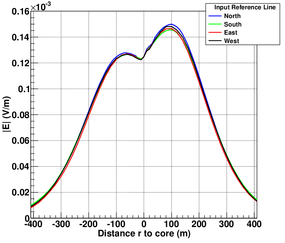
As stated earlier in this work, the choice of the reference line, where the geomagnetic and Askaryan electric fields are simulated and used as input to the model, is mostly irrelevant. This is illustrated in Fig. 8, where we show as a function of distance to core along the W-E line for the same shower geometry as in Fig. 5. Each line in Fig. 8 represents the electric field obtained from the simple model using as input one of 4 different reference lines (see legend). One can see that there is only a small dependence on the choice of the reference line, which is mostly visible in the right hand peak around m. The largest differences between the fields are obtained when comparing the N and S input reference lines. They can be understood in terms of early/late shower effects. Since the shower comes from the North, observers North of the core are closer to the shower than those at the South, inducing larger signals in the Northern reference line than in the Southern one. This effect is propagated to the predicted field amplitude of the model, which is larger when the North direction is used as input compared to that obtained with the South line as reference, for this particular shower geometry. When the West or East directions are used as input, the fields tend to fall in between the predictions obtained using the North and South reference lines as could be expected, which is particularly clear at the Cherenkov peaks. This early/late effect diminishes near the core, where the N and S antennas have equivalent distances to points along shower axis. On the other hand the effect increases as the shower zenith angle rises, since differences in distance to shower maximum from observers located N and S of the core become much more relevant.
4.3 Sources and effects of inaccuracies
Our simple model predicts the electric field to a few percent when compared to full simulations in the vast majority of shower-observer geometries as shown in Section 4.2. However, in a few particular cases the inaccuracies in the predicted field become more apparent. The main sources of inaccuracies arise from deviations from the assumptions listed in Section 3 and the extent to which each of these deviations affects the predicted electric field depends on the geometry of the shower/observer system.
One of them is related to the input of the model and the way in which separate the Askaryan and geomagnetic contributions to the electric field amplitudes (assumption C.2. in Sec. 3.1.). These could arise because the spatial structure of the shower changes as we turn off the magnetic field in the simulation and because of small differences in the time structure of the geomagnetic and Askaryan pulses. However, since in most cases we get a very good approximation of the full simulation by using the separate contributions, these errors must be small.
Early/late effects induce only very small inaccuracies in the predicted electric field in the case of low zenith angle showers, but become larger as the zenith angle increases ( at the peak for the shower shown in the bottom panel of Fig. 7).
We have checked that the geomagnetic polarization assumed in Eq. (2) describes well that obtained in full Monte Carlo simulations at all relevant distances to the shower core. However this is not the case for the Askaryan polarization at small distances to the core and manifests into larger opening angles between the expected and fully simulated polarizations. This makes our model less accurate for the prediction of the polarization of the net electric field in vertical showers in the case of observers near the shower core at distances m as can be seen in Fig. 6.
Inaccuracies also arise in the electric field amplitude predicted by the model due to the vector addition of the Askaryan and geomagnetic polarizations (Eq. 7). In fact the model is less accurate when the shower-observer geometry is such that the geomagnetic component of the emission is either smaller than the Askaryan component or has approximately the same magnitude and opposite polarization. For the geometries of the simulated showers used in this work, this occurs along the W-E line of antennas, either West or East of the core. In those geometries the model predicts a small total electric field due to the cancellation of the geomagnetic and Askaryan contributions. Several examples are shown in the right panels of Fig. 9 and represent some of the worst agreements between model and simulation of all studied showers. For instance, in the particular case of a shower coming from the North with and observers along the West to East line at the Auger site depicted in the bottom right panel, the expected Askaryan and geomagnetic polarizations are both horizontal (parallel to the W-E line), and point in opposite directions East of the core. The geomagnetic contribution dominates the emission up to , where it is equal to the Askaryan one, while for larger distances the Askaryan mechanism is slightly dominant. In this scenario, the electric field cancels in the model at a distance (East of the core). In contrast, this perfect cancellation does not occur in the simulation, as can be seen in the same figure. However, although the differences between the model and full simulations are quite evident, they are still small if compared to the peak value of for this shower (below ). These differences may be attributed to small deviations in the polarization in conjunction with the inherent and unknown uncertainties on the amplitude of the geomagnetic field due to assumption C.2 in Section 3.1. Other examples are shown in the top and middle right panels, where the Askaryan and geomagnetic fields point in opposite directions West of the core. As can also be seen in Fig. 9, these differences disappear elsewhere on the ground, where the Askaryan and geomagnetic polarizations do not have approximately opposite directions, such as West (East) of the core in the bottom (top and middle) right panel and along the whole S-N line of antennas depicted in the left panels. This means that these inaccuracies only affect observers on a very small area on the ground. In some cases the discrepancies between the assumed and fully simulated polarizations are small, but there are also regions near the core in which there is a large discrepancy in the Askaryan polarization. That can cause large errors in the electric field amplitudes in these regions as shown in the bottom panel of Fig. 6 for . In summary, these larger inaccuracies occur only if the Askaryan contribution is similar to or dominates over the geomagnetic emission, and only in regions on the ground where the two mechanisms have almost opposite polarizations.


It is important to stress that the geometries for which the differences between model and simulation are more sizeable, represent only a small fraction of the detectable showers. The reason for this is that the electric field induced in these showers typically has a small contribution from the geomagnetic emission mechanism, and as a consequence these showers are less likely to trigger an actual array of antennas. Nearly vertical showers develop much closer to the antennas and can still induce triggers in such situations despite the small radio emission, but the solid angle fraction for such showers is small. Furthermore, the largest differences between model and simulation tend to occur in regions where there is a strong destructive interference between both emission mechanisms, therefore the net electric fields are highly suppressed and less likely to be detected.
5 Discussion and conclusion
We have shown that by using standard assumptions about the polarization and symmetry properties of the electric field induced by the geomagnetic and Askaryan mechanisms, we are capable of estimating with great precision the electric field at any position on the ground, for a wide range of shower-observer geometries and on an event-by-event basis. We have shown that in the majority of cases the estimates are within just a few percent of those obtained by performing full Monte Carlo calculations of the electric field from first principles. This result represents a quantitative test on the current paradigm under which radio emission from atmospheric showers is understood, namely, that the polarized electric field due to the geomagnetic and charge-excess mechanisms interfere to produce the complex patterns observed. This effort can be seen as an approach that takes into account all the complexities of the shower radio emission in a simple manner, namely by treating the two main emission mechanisms separately and looking for symmetries that do not apply to the total net electric field.
Although not shown in this work, we expect our method to work at other energies and for other primaries besides the ones used here. We have also discussed possible sources of inaccuracies as well as features of emission and shower development not explicitly taken into account in the model. These increase the differences between the predictions and full simulations so that the accuracies reported here can be regarded as upper limits on the precision of the model. We expect that by refining the assumptions described in Section 3.1 we could further improve the accuracy of the model and better constrain the two-component paradigm of radio emission in the process.
We expect the proposed method to be very useful in many applications. It could be used as a test bench for new, more robust theoretical predictions for the characteristics of each emission mechanism. Practical applications include the study of the characteristics of the radio lateral distribution function, such as its asymmetries and their dependence on shower parameters, and experimental reconstructions that are based on Monte Carlo simulations of the radio emission, such as the reconstruction of the LOFAR experiment [12].
An obvious advantage of using the method described in this work is a significant reduction in computing time. As an illustration we note that the two-dimensional map of the electric field on the ground shown in Fig. 4 required only 36 antenna positions East of the core as input77 7 This number of antennas has not been yet optimized and can be significantly further reduced.. The total computing time used for the input simulations was around 10 h in a single processor. The input was used to estimate the field at antennas at every 2 m in a rectangular grid (totalling around 200 thousand antennas) in a few minutes. Our approach could also be a faster alternative to interpolation techniques.
With our model the development and use of extensive parameterizations could be largely simplified. Parameterizations are now reduced to two simple functions for each shower (the values of as a function of distance along the reference line for each of the two mechanisms). Such calculations could be used to study more subtle effects such as shower to shower fluctuations or those attributed to different hypotheses about composition or hadronic model.
6 Acknowledgments
J.A.M., W.R.C and E.Z. are supported by Ministerio de Economía (PRI-PRIMASP-2011-1154 and FPA2012-39489),the Consolider-Ingenio 2010 CPAN Programme (CSD2007-00042) and Xunta de Galicia, Consellería de Educación - Grupos de Referencia Competitivos (GRC2013-024), Feder Funds, Spain and Marie Curie-IRSES/EPLANET(European Particle physics Latin American NETwork), European Union 7th Framework Program, Grant No. PIRSES-2009-GA-246806. H.S. is supported by Office of Science, U.S. Department of Energy and N.A.S.A. We thank CESGA (Centro de Supercomputación de Galicia) for computing resources.
References
- [1] T. Huege, Proceedings of the ICRC, Rio de Janeiro, Brazil (2013), available in arXiv:1310.6927 [astro-ph] (2013).
- [2] M. Nagano, A. Watson, Rev. Mod. Phys. 72 (2000) 689, and references therein.
- [3] F.G. Schröder for the Pierre Auger Collaboration, Proceedings of the ICRC, Rio de Janeiro, Brazil (2013), #0899.
- [4] R. Gaior for the Pierre Auger Collaboration, Proceedings of the ICRC, Rio de Janeiro, Brazil (2013), #0883
- [5] J. Abraham et al [Auger Collaboration], NIMA, 523 (2004) 50.
- [6] D. Ardouin et al. [CODALEMA Collaboration], Astropart. Phys. 31 (2009) 192.
- [7] A. Nigl et al. [LOPES Collaboration], Astron. Astrophys. 488, 807 (2008).
- [8] D. Ardouin et al. [TREND Collaboration] Astropart. Phys. 34 717 (2011) 717; O. Martineau-Huynh for the TREND Collaboration, arXiv:1204.1599 [astro-ph].
- [9] P. Schellart et al. [LOFAR Collaboration], Astron. & Astrophys. 560 (2013) A98.
- [10] F.G. Schröder for the Tunka-Rex Collaboration, Proceedings of the ICRC, Rio de Janeiro, Brazil (2013), #0452.
- [11] W.D. Apel et al. [KASCADE & LOPES Collaborations] Phys. Rev. D 85 (2012) 071101(R).
- [12] S. Buitink et al. [LOFAR Collaboration], Proceedings of the ICRC, Rio de Janeiro, Brazil (2013), #0579.
- [13] H.R. Allan, R.W. Clay, J.K. Jones, Nature 227 (1970) 1116.
- [14] W.D. Apel et al. [KASCADE & LOPES Collaborations] Astropart. Phys. 32 (2010) 294.
- [15] S. Hoover et al. [ANITA Collaboration], Phys. Rev. Lett. 105 (2010) 151101.
- [16] R. Smida et al. [CROME group], arXiv:1306.6738 [astro-ph] (2013).
- [17] O. Scholten, K. Werner, F. Rusydi, Astropart. Phys. 29 (2008) 94; K. Werner, O. Scholten, Astropart. Phys. 29 (2008) 393.
- [18] K. Werner, K. D. de Vries, O. Scholten, Astropart. Phys. 37 (2012) 5
- [19] M. Ludwig, T. Huege, Astropart. Phys. 34, 438 (2011).
- [20] V. Marin and B. Revenu, Astropart. Phys. 35 (2012) 733.
- [21] J. Alvarez-Muñiz, W.R. Carvalho, E. Zas, Astropart. Phys. 35 (2012) 325.
- [22] T. Huege, C.W. James, Proceedings of the ICRC 2013, Rio de Janeiro, Brazil (2013) #548.
- [23] J. Alvarez-Muñiz, W.R. Carvalho, A. Romero-Wolf, M. Tueros and E. Zas, Phys. Rev. D 86 (2012) 123007
- [24] J. Alvarez-Mu˜niz, W.R. Carvalho Jr., A. Romero-Wolf, M. Tueros and E. Zas, Proceedings of the ICRC 2013, Rio de Janeiro, Brazil (2013) #105.
- [25] T. Huege, AIP Conf. Proc. 1535 (2013) 121, avaiable in 1301.2135 [astro-ph]
- [26] W.D. Apel et al. [LOPES Collaboration] Astropart. Phys. 50-52 (2013) 76
- [27] A. Aab et al. [Pierre Auger Collaboration] Phys. Rev. D 89, 052002 (2014).
- [28] T. Huege, R. Ulrich, R. Engel, Astropart. Phys. 30 (2008) 96.
- [29] N.N. Kalmykov and A.A. Konstantinov JCAP 12 (2012) 029
- [30] K.D. de Vries, A.M. van den Berg, O. Scholten, K. Werner, Astropart. Phys. 34 (2010) 267.
- [31] K. D. de Vries, O. Scholten, K. Werner, Astropart. Phys. 45 (2013) 23–27.
- [32] A. Nelles et al. arXiv:1402.2872 [astro-ph]
- [33] H. R. Allan, in: J. G. Wilson, S. A. Wouthuysen (Eds.), Progress in Elementary Particle and Cosmic Ray Physics 10, North Holland, (1971), p. 169, and refs. therein.
- [34] J.R. Prescott, J.H. Hough, and J.K. Pidcock, Nature Phys. Science 233 (1971) 109.
- [35] G.A. Askar’yan, Soviet Physics JETP 14 (1962) 441; G. A. Askaryan, Soviet Phys. JETP 21 (1965) 658.
- [36] F.D. Kahn, I. Lerche, Proc. Roy. Soc. A289 (1966) 206.
- [37] J.D. Jackson, “Classical Electrodynamics” Ed. (Wiley, New York, 1998).
- [38] E. Zas, F. Halzen, T. Stanev, Phys. Rev. D 45 (1992) 362.
- [39] F. Halzen, E. Zas, T. Stanev, Phys. Lett. B 257 (1991) 432.
- [40] D. García-Fernández, J. Alvarez-Muñiz, W.R. Carvalho Jr., A. Romero-Wolf, E. Zas, Phys. Rev. D 87 (2013) 023003.
- [41] K. D. de Vries, A. M. van den Berg, O. Scholten, K. Werner Phys. Rev. Lett. 107 (2011) 061101