On the Convergence of Approximate Message Passing with Arbitrary MatricesThanks: S. Rangan (email: srangan@nyu.edu) is with the Department of Electrical and Computer Engineering, New York University, Brooklyn, NY, 11201. His work was supported in part by the National Science Foundation under Grant 1116589 and the industrial affiliates of NYU WIRELESS.Thanks: A. K. Fletcher (email: akfletcher@ucla.edu) is with the Department of Statistics and Electrical Engineering, the University of California, Los Angeles, CA, 90095. Her work was supported in part by the National Science Foundation under Grant 1254204 and the Office of Naval Research under Grant N00014-15-1-2677.Thanks: P. Schniter and S. Sarkar (email: schniter@ece.osu.edu and sarkar.51@osu.edu) are with the Department of Electrical and Computer Engineering, The Ohio State University, Columbus, OH, 43210. Their work was supported in part by the National Science Foundation under Grants CCF-1018368, CCF-1218754, and CCF-1527162.Thanks: Portions of this work were presented at the IEEE International Symposium on Information Theory [1].

Sundeep Rangan Philip Schniter Alyson K. Fletcher Subrata Sarkar Affiliation:

Abstract

Approximate message passing (AMP) methods and their variants have attracted considerable recent attention for the problem of estimating a random vector $\mathbf{x}$ observed through a linear transform $\mathbf{A}$ . In the case of large i.i.d. zero-mean Gaussian $\mathbf{A}$ , the methods exhibit fast convergence with precise analytic characterizations on the algorithm behavior. However, the convergence of AMP under general transforms $\mathbf{A}$ is not fully understood. In this paper, we provide sufficient conditions for the convergence of a damped version of the generalized AMP (GAMP) algorithm in the case of quadratic cost functions (i.e., Gaussian likelihood and prior). It is shown that, with sufficient damping, the algorithm is guaranteed to converge, although the amount of damping grows with peak-to-average ratio of the squared singular values of the transforms $\mathbf{A}$ . This result explains the good performance of AMP on i.i.d. Gaussian transforms $\mathbf{A}$ , but also their difficulties with ill-conditioned or non-zero-mean transforms $\mathbf{A}$ . A related sufficient condition is then derived for the local stability of the damped GAMP method under general cost functions, assuming certain strict convexity conditions.

Index Terms:

Approximate message passing, loopy belief propagation, Gaussian belief propagation, primal-dual algorithms.

I Introduction

Consider estimating a random vector $\mathbf{x}\in{\mathbb{R}}^{n}$ with independent components $x_{j}\sim P(x_{j})$ from observations $\mathbf{y}\in{\mathbb{R}}^{m}$ that are conditionally independent given the transform outputs

\mathbf{z}=\mathbf{A}\mathbf{x},

(1)

i.e., $P(\mathbf{y}|\mathbf{z})=\prod_{i}P(y_{i}|z_{i})$ . Here, we assume knowledge of the matrix $\mathbf{A}\in{\mathbb{R}}^{m\times n}$ in (1) and the densities $P(x_{j})$ and $P(y_{i}|z_{i})$ . Often, the goal is to compute either the minimum mean-squared error (MMSE) estimate $\widehat{\mathbf{x}}_{\text{\sf MMSE}}=\int_{{\mathbb{R}}^{n}}\!\mathbf{x}\,P(\mathbf{x}|\mathbf{y})\mathop{}\!\mathrm{d}\mathbf{x}=\mathbb{E}(\mathbf{x}|\mathbf{y})$ or the maximum a posteriori (MAP) estimate $\widehat{\mathbf{x}}_{\text{\sf MAP}}=\mathop{\mathrm{arg\,max}}_{\mathbf{x}\in{\mathbb{R}}^{n}}P(\mathbf{x}|\mathbf{y})$ , where in either case $P(\mathbf{x}|\mathbf{y})$ denotes the posterior distribution. Using $F(\mathbf{z}):=-\ln P(\mathbf{y}|\mathbf{z})$ and $G(\mathbf{x}):=-\ln P(\mathbf{x})$ and Bayes rule, $P(\mathbf{x}|\mathbf{y})\propto P(\mathbf{y}|\mathbf{x})P(\mathbf{x})$ , it becomes evident that MAP estimation is equivalent to the optimization problem

\displaystyle\widehat{\mathbf{x}}_{\text{\sf MAP}}=\mathop{\mathrm{arg\,min}}_{\mathbf{x}\in{\mathbb{R}}^{n}}F(\mathbf{A}\mathbf{x})+G(\mathbf{x})

(2)

for separable $F(\mathbf{z})=\sum_{i}F_{i}(z_{i})$ and $G(\mathbf{x})=\sum_{j}G_{j}(x_{j})$ . Such problems arise in a range of applications including statistical regression, inverse problems, and compressed sensing.

Most current numerical methods for solving the constrained optimization problem (2) attempt to exploit the separable structure of the objective function (2) using approaches like iterative shrinkage and thresholding (ISTA) [2, 3, 4, 5, 6, 7], the alternating direction method of multipliers (ADMM) [8, 9, 10, 11], or primal-dual approaches [9, 10, 11, 12].

In recent years, however, there has also been considerable interest in approximate message passing (AMP) methods that apply Gaussian and quadratic approximations to loopy belief propagation (BP) in graphical models [13, 14, 15]. AMP applied to max-sum loopy BP produces a sequence of estimates that approximate $\widehat{\mathbf{x}}_{\text{\sf MAP}}$ , while AMP applied to sum-product loopy BP produces a sequence of estimates that approximate $\widehat{\mathbf{x}}_{\text{\sf MMSE}}$ . For zero-mean i.i.d. sub-Gaussian $\mathbf{A}$ in the large-system limit (i.e., $m,n\rightarrow\infty$ with fixed $m/n$ ), AMP methods are characterized by a state evolution whose fixed points, when unique, coincide with $\widehat{\mathbf{x}}_{\text{\sf MAP}}$ or $\widehat{\mathbf{x}}_{\text{\sf MMSE}}$ [16, 17, 18]. In addition, for large but finite-sized i.i.d. Gaussian matrices, recent work [19] shows that AMP is close to Bayes-optimal.

Unfortunately, a rigorous characterization of AMP for generic $\mathbf{A}$ remains lacking. The recent papers [20, 21] studied the fixed-points of the generalized AMP (GAMP) algorithm from [15] for generic $\mathbf{A}$ . In [20], it was established that the fixed points of max-sum GAMP coincide with the critical points of the optimization objective in (2). Similarly, [20, 21] established that the fixed points of sum-product GAMP are critical points of a large-system version of the Bethe free energy from [22]. However, the papers [20, 21] did not discuss the convergence of the algorithm to those fixed points. Indeed, similar to other loopy BP algorithms, GAMP may diverge, as demonstrated for mildly ill-conditioned $\mathbf{A}$ in [23]. Likewise, [24] showed that AMP can diverge with non-zero-mean i.i.d. Gaussian $\mathbf{A}$ and the divergence can, in fact, be predicted via a state-evolution analysis.

For general loopy BP, a variety of methods have been proposed to improve convergence, including coordinate descent, tree re-weighting, and double loop methods [25, 26, 27, 28, 29]. In this paper, we propose and analyze a “damped” modification of GAMP that is similar to the technique used in Gaussian belief propagation [30, 31]—a closely related algorithm. We also point out connections between damped GAMP and the primal-dual hybrid-gradient (PDHG) algorithm [9, 10, 11, 12] popular in convex optimization. This connection enhances the interpretability of AMP methods, especially for those who are less familiar with belief propagation.

Our first main result establishes a necessary and sufficient condition on the global convergence of damped GAMP for arbitrary $\mathbf{A}$ in the special case of Gaussian $P(x_{j})$ and $P(y_{i}|z_{i})$ (i.e., quadratic $F$ and $G$ ) and fixed scalar stepsizes. This condition (see Theorem 2 below) shows that, with sufficient damping, the Gaussian GAMP algorithm can be guaranteed to converge. However, the amount of damping grows with the peak-to-average ratio of the squared singular values of $\mathbf{A}$ . This result explains why Gaussian GAMP converges (with high probability) for large i.i.d. Gaussian $\mathbf{A}$ , but it also explains why it needs to be damped significantly for non-zero-mean, low-rank, or otherwise ill-conditioned $\mathbf{A}$ .

Our second result establishes the local convergence of GAMP for strictly convex $F$ and $G$ and arbitrary, but fixed, vector-valued stepsizes. This sufficient condition is similar to the Gaussian case, but involves a certain row-column normalized version of $\mathbf{A}$ . (See Theorem 3 below.)

Finally, we present numerical experiments that verify the tightness of the sufficient conditions from Theorems 2 and 3.

Notation: We use capital boldface letters like $\mathbf{A}$ for matrices, small boldface letters like $\mathbf{a}$ for vectors, $(\cdot)^{\text{\sf T}}$ for transposition, $(\cdot)^{\text{\sf H}}$ for Hermitian (i.e., conjugate transposition), and $a_{i}=[\mathbf{a}]_{i}$ to denote the $i$ th element of $\mathbf{a}$ . Also, we use $\|\mathbf{A}\|_{2}$ for the spectral norm of $\mathbf{A}$ , $\|\mathbf{A}\|_{F}$ for the Frobenius norm of $\mathbf{A}$ , and $\mathop{\mathrm{Diag}}(\mathbf{a})$ for the diagonal matrix created from vector $\mathbf{a}$ . In addition, we use $\mathbf{0}$ for the all-zeros vector, $\mathbf{1}$ for the all-ones vector, and $\mathbf{I}_{N}$ for the $N\times N$ identity matrix. Although it is somewhat non-standard, we use $\mathbf{A}.\mathbf{B}$ for component-wise multiplication, $\mathbf{A}./\mathbf{B}$ for component-wise division of the matrices $\mathbf{A}$ and $\mathbf{B}$ , and $|\mathbf{A}|$ for component-wise magnitude of $\mathbf{A}$ . Similarly, we use $\mathbf{a}\geq\mathbf{0}$ to denote component-wise inequality (i.e., $a_{i}\geq 0$ for $i=1,..,n$ ). For a random vector $\mathbf{x}$ , we denote its probability density function (pdf) by $P(\mathbf{x})$ , and its expectation by $\mathbb{E}[\mathbf{x}]$ . Similarly, we use $P(\mathbf{x}|\mathbf{y})$ and $\mathbb{E}[\mathbf{x}|\mathbf{y}]$ for the conditional pdf and expectation, respectively. We refer to the pdf of a Gaussian random vector $\mathbf{x}\in{\mathbb{R}}^{N}$ with mean $\mathbf{a}$ and covariance $\mathbf{R}$ using ${\mathcal{N}}(\mathbf{x};\mathbf{a},\mathbf{R})=\exp(-(\mathbf{x}-\mathbf{a})^{\text{\sf T}}\mathbf{R}^{-1}(\mathbf{x}-\mathbf{a})/2)/\sqrt{(2\pi)^{N}|\mathbf{R}|}$ . Finally, $P(\mathbf{x})\propto Q(\mathbf{x})$ says that functions $P(\cdot)$ and $Q(\cdot)$ are equal up to a scaling that is invariant to $\mathbf{x}$ .

II Damped GAMP

II-A Review of GAMP

The GAMP algorithm was introduced in [15] and rigorously analyzed in [17]. The procedure (see Algorithm 1) produces a sequence of estimates $\widehat{\mathbf{x}}^{t},t=1,2,\dots$ , that, in max-sum mode, approximate $\widehat{\mathbf{x}}_{\text{\sf MAP}}$ and, in sum-product mode, approximate $\widehat{\mathbf{x}}_{\text{\sf MMSE}}$ . The two modes differ only in the definition of the scalar estimation functions ${g}_{s}$ and $g_{x}$ used in lines 8, 9, 12, and 13 of Algorithm 1:

•

In max-sum mode,

	$\displaystyle{[g_{x}(\mathbf{r},\bm{{\color[rgb]{0,0,0}\tau}}_{r})]}_{j}$	$\displaystyle=$	$\displaystyle\prox_{\tau_{r_{j}}G_{j}}(r_{j})$		(3)
	$\displaystyle{[{g}_{s}({\mathbf{p}},{\color[rgb]{0,0,0}\bm{\nu}}_{p})]}_{i}$	$\displaystyle=$	$\displaystyle{p}_{i}-\nu_{p_{i}}\prox_{F_{i}/\nu_{p_{i}}}({p}_{i}/\nu_{p_{i}})$		(4)

using $\bm{{\color[rgb]{0,0,0}\tau}}_{r}=[\tau_{r_{1}},\dots,\tau_{r_{n}}]^{\text{\sf T}}$ , ${\color[rgb]{0,0,0}\bm{\nu}}_{p}=[\nu_{p_{1}},\dots,\nu_{p_{m}}]^{\text{\sf T}}$ , and

\prox_{f}(r):=\mathop{\mathrm{arg\,min}}_{x}f(x)+\tfrac{1}{2}|x-r|^{2}.

(5)

Note (3) implements scalar MAP denoising under prior $P(x_{j})\!\propto\!\exp(-G(x_{j}))$ and variance- $\tau_{r_{j}}$ Gaussian noise.

•

In sum-product mode,

	$\displaystyle{[g_{x}(\mathbf{r},\bm{{\color[rgb]{0,0,0}\tau}}_{r})]}_{j}$	$\displaystyle=$	$\displaystyle\frac{\int x_{j}P(x_{j})\mathcal{N}(x_{j};r_{j},\tau_{r_{j}})\mathop{}\!\mathrm{d}x_{j}}{\int P(x_{j})\mathcal{N}(x_{j};r_{j},\tau_{r_{j}})\mathop{}\!\mathrm{d}x_{j}}$		(6)
	$\displaystyle{[{g}_{s}({\mathbf{p}},{\color[rgb]{0,0,0}\bm{\nu}}_{p})]}_{i}$	$\displaystyle=$	$\displaystyle{p}_{i}-\nu_{p_{i}}\frac{\int z_{i}P(y_{i}\|z_{i})\mathcal{N}(z_{i};\frac{{p}_{i}}{\nu_{p_{i}}},\frac{1}{\nu_{p_{i}}})\mathop{}\!\mathrm{d}z_{i}}{\int P(y_{i}\|z_{i})\mathcal{N}(z_{i};\frac{{p}_{i}}{\nu_{p_{i}}},\frac{1}{\nu_{p_{i}}})\mathop{}\!\mathrm{d}z_{i}},$

and so (6) is the scalar MMSE denoiser under $P(x_{j})\!\propto\!\exp(-G(x_{j}))$ and variance- $\tau_{r_{j}}$ Gaussian noise.

Note that, in Algorithm 1 and the sequel, $\mathbf{a}.\mathbf{b}$ and $\mathbf{a}./\mathbf{b}$ denote component-wise multiplication and division, respectively, between vectors $\mathbf{a}$ and $\mathbf{b}$ .

Algorithm 1 GAMP with vector stepsizes and damping

0: Matrix

\mathbf{A}

, scalar estimation functions

g_{x}

and

{g}_{s}

, and damping constants

\theta_{s},\theta_{x}\in(0,1]

\mathbf{S}=\mathbf{A}.\mathbf{A}

(component-wise magnitude squared)

t=0

3: Initialize

\bm{{\color[rgb]{0,0,0}\tau}}_{x}^{t}>\mathbf{0}

\mathbf{x}^{t}

{\mathbf{s}}^{t\!-\!1}=\mathbf{0}

5: repeat

\mathbf{1}./{\color[rgb]{0,0,0}\bm{\nu}}_{p}^{t}=\mathbf{S}\bm{{\color[rgb]{0,0,0}\tau}}_{x}^{t}

{\mathbf{p}}^{t}={\mathbf{s}}^{t\!-\!1}+{\color[rgb]{0,0,0}\bm{\nu}}_{p}^{t}.\mathbf{A}\mathbf{x}^{t}

{\color[rgb]{0,0,0}\bm{\nu}}_{s}^{t}={\color[rgb]{0,0,0}\bm{\nu}}_{p}^{t}.{g}_{s}^{\prime}({\mathbf{p}}^{t},{\color[rgb]{0,0,0}\bm{\nu}}_{p}^{t})

{\mathbf{s}}^{t}=(1-\theta_{s}){\mathbf{s}}^{t\!-\!1}+\theta_{s}{g}_{s}({\mathbf{p}}^{t},{\color[rgb]{0,0,0}\bm{\nu}}^{t}_{p})

10:

\mathbf{1}./\bm{{\color[rgb]{0,0,0}\tau}}_{r}^{t}=\mathbf{S}^{\text{\sf T}}{\color[rgb]{0,0,0}\bm{\nu}}_{s}^{t}

11:

\mathbf{r}^{t}=\mathbf{x}^{t}-\bm{{\color[rgb]{0,0,0}\tau}}^{t}_{r}.\mathbf{A}^{\text{\sf H}}{\mathbf{s}}^{t}

12:

\bm{{\color[rgb]{0,0,0}\tau}}^{t\!+\!1}_{x}=\bm{{\color[rgb]{0,0,0}\tau}}^{t}_{r}.g_{x}^{\prime}(\mathbf{r}^{t},\bm{{\color[rgb]{0,0,0}\tau}}^{t}_{r})

13:

\mathbf{x}^{t\!+\!1}=(1-\theta_{x})\mathbf{x}^{t}+\theta_{x}g_{x}(\mathbf{r}^{t},\bm{{\color[rgb]{0,0,0}\tau}}^{t}_{r})

14:

t\leftarrow t+1

15: until Terminated

Algorithm 1 reveals the computational efficiency of GAMP: the vector-valued MAP and MMSE estimation problems are reduced to a sequence of scalar estimation problems in Gaussian noise. Specifically, each iteration involves multiplications by $\mathbf{S}$ , $\mathbf{S}^{\text{\sf T}}$ , $\mathbf{A}$ and $\mathbf{A}^{\text{\sf H}}$ along with simple scalar estimations on the components $x_{j}$ and $z_{i}$ ; there are no vector-valued estimations or matrix inverses.

We note that Algorithm 1 writes GAMP in a “symmetrized” form, where the steps in lines 6-9 mirror those in lines 10-13. This differs from the way that GAMP is presented in most other publications, such as [15], which is obtained by replacing the variables $\mathbf{s}$ , ${\color[rgb]{0,0,0}\bm{\nu}}_{p}$ , and $\mathbf{p}$ in Algorithm 1 by $-\mathbf{s}$ , $\mathbf{1}./\bm{{\color[rgb]{0,0,0}\tau}}_{p}$ , and $\mathbf{p}.\bm{{\color[rgb]{0,0,0}\tau}}_{p}$ , respectively. Note that, thoughout this paper, we use $\tau$ for variance quantities and $\nu$ for precision (i.e., inverse variance) quantities.

II-B Damped GAMP

Algorithm 1 includes a small but important modification to the original GAMP from [15]: lines 9 and 13 perform damping using constants $\theta_{s},\theta_{x}\in(0,1]$ that slow the updates of $\mathbf{s}^{t},\mathbf{x}^{t}$ when $\theta_{s},\theta_{x}<1$ , respectively. The original GAMP implicitly uses $\theta_{s}=1=\theta_{x}$ . In the sequel, we establish—analytically—that damping facilitates the convergence of GAMP for general $\mathbf{A}$ , a fact that has been empirically observed in past works (e.g., [32, 24, 23]).

II-C GAMP with Scalar Stepsizes

The computational complexity of Algorithm 1 is dominated by the matrix-vector multiplications involving $\mathbf{A}$ , $\mathbf{A}^{\text{\sf H}}$ , $\mathbf{S},$ and $\mathbf{S}^{\text{\sf T}}$ . In [33], a scalar-stepsize simplification of GAMP was proposed to avoid the multiplications by $\mathbf{S}$ and $\mathbf{S}^{\text{\sf T}}$ , roughly halving the per-iteration complexity. The meaning of “stepsize” will become clear in the sequel. Algorithm 2 shows the scalar-stepsize version of Algorithm 1.

For use in the sequel, we now show that scalar-stepsize GAMP is equivalent to vector-stepsize GAMP under a different choice of $\mathbf{S}$ . While Algorithm 1 uses $\mathbf{S}=\mathbf{A}.\mathbf{A}$ , Algorithm 2 effectively uses

\mathbf{S}=\frac{\|\mathbf{A}\|_{F}^{2}}{mn}\mathbf{1}\mathbf{1}^{\text{\sf T}},

(7)

i.e., a constant matrix having the same average value as $\mathbf{A}.\mathbf{A}$ . Thus, the two algorithms coincide when $|A_{ij}|$ is invariant to $i$ and $j$ . To see the equivalence, we first note that, under $\mathbf{S}$ from (7), line 6 in Algorithm 1 would produce a version of $1/{\color[rgb]{0,0,0}\bm{\nu}}_{p}^{t}$ containing identical elements $1/\nu_{p}^{t}$ , where

\frac{1}{\nu_{p}^{t}}=\frac{\|\mathbf{A}\|_{F}^{2}}{mn}\mathbf{1}^{\text{\sf T}}\bm{{\color[rgb]{0,0,0}\tau}}_{x}^{t}=\frac{\|\mathbf{A}\|_{F}^{2}}{m}\tau_{x}^{t}

for $\tau_{x}^{t}=(1/n)\mathbf{1}^{\text{\sf T}}\bm{{\color[rgb]{0,0,0}\tau}}_{x}$ . Similarly, line 10 would produce a vector $1/\bm{{\color[rgb]{0,0,0}\tau}}_{r}^{t}$ with identical elements $1/\tau_{r}^{t}$ , where

\frac{1}{\tau_{r}^{t}}=\frac{\|\mathbf{A}\|_{F}^{2}}{mn}\mathbf{1}^{\text{\sf T}}{\color[rgb]{0,0,0}\bm{\nu}}_{s}^{t}=\frac{\|\mathbf{A}\|_{F}^{2}}{n}\nu_{s}^{t},

for $\nu_{s}^{t}=(1/m)\mathbf{1}^{\text{\sf T}}{\color[rgb]{0,0,0}\bm{\nu}}_{s}^{t}$ . Furthermore, ${\color[rgb]{0,0,0}\bm{\nu}}_{p}^{t}=\nu_{p}^{t}\mathbf{1}$ and line 8 imply that $\nu_{s}^{t}=(\nu_{p}^{t}/m)\mathbf{1}^{\text{\sf T}}{g}_{s}({\mathbf{p}}^{t},{\color[rgb]{0,0,0}\bm{\nu}}_{p}^{t})$ , while $\bm{{\color[rgb]{0,0,0}\tau}}_{r}^{t}=\tau_{r}^{t}\mathbf{1}$ and line 12 imply that $\tau_{x}^{t\!+\!1}=(\tau_{r}^{t}/n)\mathbf{1}^{\text{\sf T}}g_{x}(\mathbf{r}^{t},\bm{{\color[rgb]{0,0,0}\tau}}_{r}^{t})$ . Applying these modifications to Algorithm 1, we arrive at Algorithm 2.

Algorithm 2 GAMP with scalar stepsizes and damping

0: Matrix

\mathbf{A}

, scalar estimation functions

g_{x}

and

{g}_{s}

, and damping constants

\theta_{s},\theta_{x}\in(0,1]

t=0

2: Initialize

\tau_{x}^{t}>0

\mathbf{x}^{t}

{\mathbf{s}}^{t\!-\!1}=\mathbf{0}

4: repeat

1/\nu_{p}^{t}=(1/m)\|\mathbf{A}\|_{F}^{2}\tau_{x}^{t}

{\mathbf{p}}^{t}={\mathbf{s}}^{t\!-\!1}+\nu_{p}^{t}\mathbf{A}\mathbf{x}^{t}

\nu_{s}^{t}=(\nu_{p}^{t}/m)\mathbf{1}^{\text{\sf T}}{g}_{s}^{\prime}({\mathbf{p}}^{t},\nu_{p}^{t})

{\mathbf{s}}^{t}=(1-\theta_{s}){\mathbf{s}}^{t\!-\!1}+\theta_{s}{g}_{s}({\mathbf{p}}^{t},\nu_{p}^{t})

1/\tau_{r}^{t}=(1/n)\|\mathbf{A}\|^{2}_{F}\nu_{s}^{t}

10:

\mathbf{r}^{t}=\mathbf{x}^{t}-\tau^{t}_{r}\mathbf{A}^{\text{\sf H}}{\mathbf{s}}^{t}

11:

\tau^{t\!+\!1}_{x}=(\tau^{t}_{r}/n)\mathbf{1}^{\text{\sf T}}g_{x}^{\prime}(\mathbf{r}^{t},\tau^{t}_{r})

12:

\mathbf{x}^{t\!+\!1}=(1-\theta_{x})\mathbf{x}^{t}+\theta_{x}g_{x}(\mathbf{r}^{t},\tau^{t}_{r})

13:

t\leftarrow t+1

14: until Terminated

II-D Relation to Primal-Dual Hybrid Gradient Algorithms

An important case of (2) is when $F$ and $G$ are closed proper convex functionals and the solution $\widehat{\mathbf{x}}_{\text{\sf MAP}}$ exists. Recently, there has been great interest in solving this problem from the primal-dual perspective [9, 12], which can be described as follows. Consider $F^{*}$ , the convex conjugate of $F$ , as given by the Legendre-Fenchel transform

F^{*}(\mathbf{s}):=\sup_{\mathbf{z}\in{\mathbb{R}}^{m}}\mathbf{s}^{\text{\sf T}}\mathbf{z}-F(\mathbf{z}).

(8)

For closed proper convex $F$ , we have $F^{**}=F$ , and so

F(\mathbf{A}\mathbf{x})=\sup_{\mathbf{s}\in{\mathbb{R}}^{m}}\mathbf{s}^{\text{\sf T}}\mathbf{A}\mathbf{x}-F^{*}(\mathbf{s}),

(9)

which gives the equivalent saddle-point formulation of (2),

\min_{\mathbf{x}\in{\mathbb{R}}^{n}}\sup_{\mathbf{s}\in{\mathbb{R}}^{m}}\mathbf{s}^{\text{\sf T}}\mathbf{A}\mathbf{x}-F^{*}(\mathbf{s})+G(\mathbf{x}).

(10)

The so-called primal-dual hybrid-gradient (PDHG) algorithm recently studied in [9, 10, 11, 12] is defined by the iteration

$\displaystyle{\mathbf{s}}^{t}$	$\displaystyle\leftarrow$	$\displaystyle\prox_{\nu_{p}F^{*}}\big({\mathbf{s}}^{t-1}+\nu_{p}\mathbf{A}\mathbf{x}^{t}\big)$	(11)
$\displaystyle\widehat{\mathbf{x}}^{t\!+\!1}$	$\displaystyle\leftarrow$	$\displaystyle\prox_{\tau_{r}G}\big(\widehat{\mathbf{x}}^{t}-\tau_{r}\mathbf{A}^{\text{\sf H}}{\mathbf{s}}^{t}\big)$	(12)
$\displaystyle\mathbf{x}^{t\!+\!1}$	$\displaystyle\leftarrow$	$\displaystyle\widehat{\mathbf{x}}^{t\!+\!1}+\theta(\widehat{\mathbf{x}}^{t\!+\!1}-\widehat{\mathbf{x}}^{t}),$	(13)

where $\theta\in[-1,1]$ is a relaxation parameter. Line (11) can be recognized as proximal gradient ascent in the dual variable ${\mathbf{s}}$ using stepsize $\nu_{p}$ , while line (12) is proximal gradient descent in the primal variable $\mathbf{x}$ using stepsize $\tau_{r}$ .

PDHG can be related to damped scalar-stepsize GAMP as follows. Since $F$ is proper, closed, and convex, we can apply the Moreau identity [34]

{\mathbf{p}}=\prox_{{\color[rgb]{0,0,0}\bm{\nu}}_{p}F^{*}}({\mathbf{p}})+{\color[rgb]{0,0,0}\bm{\nu}}_{p}\prox_{F/{\color[rgb]{0,0,0}\bm{\nu}}_{p}}({\mathbf{p}}/{\color[rgb]{0,0,0}\bm{\nu}}_{p})

(14)

to (4), after which the assumed separability of $F$ implies that

[{g}_{s}({\mathbf{p}},{\color[rgb]{0,0,0}\bm{\nu}}_{p})]_{i}=\prox_{\nu_{p_{i}}F_{i}^{*}}({p}_{i}).

(15)

Thus, under $\theta_{s}=1$ , scalar GAMP’s update of ${\mathbf{s}}$ (in line 8 of Algorithm 2) matches PDHG’s in (11). Similarly, noting the connection between (3) and (12), it follows that, under $\theta_{x}=1$ , scalar GAMP’s update of $\mathbf{x}$ (in line 12 of Algorithm 2)) matches the PDHG update (13) under $\theta=0$ .

In summary, PDHG under $\theta=0$ (the Arrow-Hurwicz [35] case) would be equivalent to non-damped scalar GAMP if the stepsizes $\nu_{p}^{t}$ and $\tau_{r}^{t}$ were fixed over the iterations. GAMP, however, adapts these stepsizes. In fact, under the existence of the second derivative $f^{\prime\prime}$ , it can be shown that

\prox^{\prime}_{f}(r)=\big[1+f^{\prime\prime}\big(\prox_{f}(r)\big)\big]^{-1},

(16)

implying that, for smooth $F$ and $G$ , GAMP updates $\tau_{x}^{t}$ according to the average local curvature of $G$ at the point $\mathbf{x}=\prox_{\tau_{r}^{t}G}(\mathbf{r}^{t})$ and updates $\nu_{s}^{t}$ according to the average local curvature of $F^{*}$ at the point ${\mathbf{s}}=\prox_{\nu_{p}^{t}F^{*}}({\mathbf{p}}^{t})$ . A different form of PDHG stepsize adaptation has been recently considered in [36], one that is not curvature based.

Meanwhile, PDHG under $\theta\neq 0$ is similar to fixed-stepsize damped scalar GAMP with $\theta_{s}=1$ and $\theta_{x}=1+\theta$ , although not the same. Note that PDHG uses the damped version of $\mathbf{x}$ only in the dual update (11) whereas GAMP uses the damped version of $\mathbf{x}$ in both primal and dual updates. Also, PDHG relaxes only the primal variable $\mathbf{x}$ , whereas damped GAMP relaxes (or damps) both primal and dual variables.

III Damped Gaussian GAMP

III-A Gaussian GAMP

Although Algorithms 1 and 2 apply to generic distributions $P(x_{j})$ and $P(y_{i}|z_{i})$ , we find it useful to at first consider the simple case of Gaussian distributions, and in particular

P(x_{j})={\mathcal{N}}(x_{j};x_{0_{j}},\tau_{0_{j}}),\quad P(y_{i}|z_{i})={\mathcal{N}}(z_{i};y_{i},\nu_{w_{i}}^{-1}),

where $\tau_{0_{j}}$ are variances and $\nu_{w_{i}}$ are precisions (i.e., inverse variances). In this case, the scalar estimation functions used in max-sum mode are identical to those in sum-product mode, and are linear [33]:


$\displaystyle{g}_{s}({\mathbf{p}},{\color[rgb]{0,0,0}\bm{\nu}}_{p})$	$\displaystyle=$	$\displaystyle{\color[rgb]{0,0,0}\bm{\nu}}_{w}.({\mathbf{p}}+{\color[rgb]{0,0,0}\bm{\nu}}_{w}.\mathbf{y})./({\color[rgb]{0,0,0}\bm{\nu}}_{p}+{\color[rgb]{0,0,0}\bm{\nu}}_{w})-{\color[rgb]{0,0,0}\bm{\nu}}_{w}.\mathbf{y}\qquad$	(17a)
$\displaystyle g_{x}(\mathbf{r},\bm{{\color[rgb]{0,0,0}\tau}}_{r})$	$\displaystyle=$	$\displaystyle\bm{{\color[rgb]{0,0,0}\tau}}_{0}.(\mathbf{r}-\mathbf{x}_{0})./(\bm{{\color[rgb]{0,0,0}\tau}}_{0}+\bm{{\color[rgb]{0,0,0}\tau}}_{r})+\mathbf{x}_{0}.$	(17b)

Henceforth, we use “Gaussian GAMP” (GGAMP) when referring to GAMP under the estimation functions (17).

III-B Convergence of GGAMP Stepsizes

We first establish the convergence of the GGAMP stepsizes in the case of an arbitrary matrix $\mathbf{A}$ . For the vector-stepsize case in Algorithm 1, lines 8 and 12 become


$\displaystyle{\color[rgb]{0,0,0}\bm{\nu}}_{s}^{t}$	$\displaystyle=$	$\displaystyle{\color[rgb]{0,0,0}\bm{\nu}}_{p}^{t}.{g}_{s}^{\prime}({\mathbf{p}}^{t},{\color[rgb]{0,0,0}\bm{\nu}}^{t}_{p})={\color[rgb]{0,0,0}\bm{\nu}}_{p}^{t}.{\color[rgb]{0,0,0}\bm{\nu}}_{w}./({\color[rgb]{0,0,0}\bm{\nu}}_{p}^{t}+{\color[rgb]{0,0,0}\bm{\nu}}_{w})$	(18a)
$\displaystyle\bm{{\color[rgb]{0,0,0}\tau}}_{x}^{t\!+\!1}$	$\displaystyle=$	$\displaystyle\bm{{\color[rgb]{0,0,0}\tau}}_{r}^{t}.g_{x}^{\prime}(\mathbf{r}^{t},\bm{{\color[rgb]{0,0,0}\tau}}_{r}^{t})=\bm{{\color[rgb]{0,0,0}\tau}}_{r}^{t}.\bm{{\color[rgb]{0,0,0}\tau}}_{0}./(\bm{{\color[rgb]{0,0,0}\tau}}_{r}^{t}+\bm{{\color[rgb]{0,0,0}\tau}}_{0}),$	(18b)

and, combining these with lines 6 and 10, we get


$\displaystyle 1./{\color[rgb]{0,0,0}\bm{\nu}}_{s}^{t}$	$\displaystyle=$	$\displaystyle\mathbf{S}\bm{{\color[rgb]{0,0,0}\tau}}_{x}^{t}+1./{\color[rgb]{0,0,0}\bm{\nu}}_{w}$	(19a)
$\displaystyle 1./\bm{{\color[rgb]{0,0,0}\tau}}_{x}^{t\!+\!1}$	$\displaystyle=$	$\displaystyle\mathbf{S}^{\text{\sf T}}{\color[rgb]{0,0,0}\bm{\nu}}_{s}^{t}+1./\bm{{\color[rgb]{0,0,0}\tau}}_{0},$	(19b)

which are invariant to $\theta_{s},\theta_{x},{\mathbf{s}}^{t}$ , and $\mathbf{x}^{t}$ . The scalar-stepsize case in Algorithm 2 is similar, and in either case, the following theorem shows that the GGAMP stepsizes always converge.

Theorem 1

Consider Algorithms 1 or 2) with Gaussian estimation functions (17) defined for any vectors ${\color[rgb]{0,0,0}\bm{\nu}}_{w}$ and $\bm{{\color[rgb]{0,0,0}\tau}}_{0}>\bm{0}$ . Then, as $t\rightarrow\infty$ , the stepsizes ${\color[rgb]{0,0,0}\bm{\nu}}_{p}^{t},{\color[rgb]{0,0,0}\bm{\nu}}_{s}^{t},\bm{{\color[rgb]{0,0,0}\tau}}_{r}^{t},\bm{{\color[rgb]{0,0,0}\tau}}_{x}^{t}$ (or their scalar versions) converge to unique fixed points that are invariant to $\theta_{s}$ and $\theta_{x}$ .

Proof:

See Appendix A. $\Box$

IV Scalar-Stepsize GGAMP Convergence

IV-A Scalar-stepsize GGAMP

An important special case that we now consider is scalar-stepsize GGAMP from Algorithm 2 under identical variances, i.e.,

{\color[rgb]{0,0,0}\bm{\nu}}_{w}=\nu_{w}\mathbf{1},\quad\bm{{\color[rgb]{0,0,0}\tau}}_{0}=\tau_{0}\mathbf{1},

(20)

for some $\nu_{w}$ and $\tau_{0}>0$ . In this case, lines 7 and 11 give


$\displaystyle\nu_{s}^{t}$	$\displaystyle=$	$\displaystyle\frac{1}{m}\mathbf{1}^{\text{\sf T}}\big({\color[rgb]{0,0,0}\bm{\nu}}_{p}^{t}.{g}_{s}^{\prime}({\mathbf{p}}^{t},{\color[rgb]{0,0,0}\bm{\nu}}_{p}^{t})\big)=\frac{\nu_{p}^{t}\nu_{w}}{\nu_{p}^{t}+\nu_{w}}$	(21a)
$\displaystyle\tau_{x}^{t\!+\!1}$	$\displaystyle=$	$\displaystyle\frac{1}{n}\mathbf{1}^{\text{\sf T}}\big(\bm{{\color[rgb]{0,0,0}\tau}}_{r}^{t}.g_{x}^{\prime}(\mathbf{r}^{t},\bm{{\color[rgb]{0,0,0}\tau}}_{r}^{t})\big)=\frac{\tau_{r}^{t}\tau_{0}}{\tau_{r}^{t}+\tau_{0}},$	(21b)

and, combining these with lines 5 and 9, we get


$\displaystyle\frac{1}{\nu_{s}^{t}}$	$\displaystyle=$	$\displaystyle\frac{1}{\nu_{p}^{t}}+\frac{1}{\nu_{w}}=\frac{1}{m}\\|\mathbf{A}\\|_{F}^{2}\tau_{x}^{t}+\frac{1}{\nu_{w}}$	(22a)
$\displaystyle\frac{1}{\tau_{x}^{t\!+\!1}}$	$\displaystyle=$	$\displaystyle\frac{1}{\tau_{r}^{t}}+\frac{1}{\tau_{0}}=\frac{1}{n}\\|\mathbf{A}\\|_{F}^{2}\nu_{s}^{t}+\frac{1}{\tau_{0}}.$	(22b)

IV-B Convergence

We now investigate the convergence of the primal and dual variables $\mathbf{x}^{t}$ and ${\mathbf{s}}^{t}$ for scalar GGAMP. Since, for this algorithm, the previous section established that, as $t\rightarrow\infty$ , the stepsizes $\nu_{p}^{t}$ and $\tau_{r}^{t}$ converge independently of $\theta_{s},\theta_{x},{\mathbf{s}}^{t}$ , and $\overline{\mathbf{x}}^{t}$ , we henceforth consider GGAMP with fixed stepsizes $\nu_{p}^{t}=\nu_{p}$ and $\tau_{r}^{t}=\tau_{r}$ , where $\nu_{p}$ and $\tau_{r}$ are the fixed points of (22) for Algorithm 2. (A generalization to arbitrary fixed stepsizes will be given in Section V.)

Theorem 2

Define

\Gamma(\theta_{s},\theta_{x}):=\begin{cases}\displaystyle\frac{2\left[(2-\theta_{s})m+\theta_{s}n\right]}{\theta_{s}\theta_{x}mn}&\text{if }m\geq n\\[8.53581pt] \displaystyle\frac{2\left[(2-\theta_{x})n+\theta_{x}m\right]}{\theta_{s}\theta_{x}mn}&\text{if }m\leq n.\end{cases}

(23)

Under Gaussian priors (i.e., (17)) with identical variances (20), scalar-stepsize GAMP from Algorithm 2 converges for any $\nu_{w}$ and $\tau_{0}>0$ when

\Gamma(\theta_{s},\theta_{x})>\|\mathbf{A}\|_{2}^{2}/\|\mathbf{A}\|_{F}^{2}.

(24)

Conversely, it diverges for large enough $\tau_{0}\nu_{w}$ when

\Gamma(\theta_{s},\theta_{x})<\|\mathbf{A}\|_{2}^{2}/\|\mathbf{A}\|_{F}^{2}.

(25)

Proof:

See Appendix C. $\Box$

Theorem 2 provides a simple necessary and sufficient condition on the convergence of scalar GGAMP. To better interpret this condition, recall that $\|\mathbf{A}\|_{2}^{2}$ is the maximum squared singular value of $\mathbf{A}$ and that $\|\mathbf{A}\|_{F}^{2}$ is the sum of the squared singular values of $\mathbf{A}$ (i.e., $\|\mathbf{A}\|^{2}_{F}=\sum_{i=1}^{\min\{m,n\}}\sigma^{2}_{i}(\mathbf{A})$ ). Thus

\kappa(\mathbf{A}):=\frac{\|\mathbf{A}\|_{2}^{2}}{\|\mathbf{A}\|^{2}_{F}/\min\{m,n\}}

(26)

is the peak-to-average ratio of the squared singular values of $\mathbf{A}$ . Convergence condition (24) can then be rewritten as

\kappa(\mathbf{A})<\kappa_{\max}(\theta_{s},\theta_{x}):=\min\{m,n\}\Gamma(\theta_{s},\theta_{x}),

(27)

meaning that, for GGAMP convergence, it is necessary and sufficient to choose $\kappa_{\max}(\theta_{s},\theta_{x})$ above the peak-to-average ratio of the squared singular values.

When there is no damping (i.e., $\theta_{s}=1=\theta_{x}$ ), the definitions in (23) and (27) can be combined to yield

\kappa_{\max}(1,1)=\frac{2\min\{m,n\}(m+n)}{mn}\in(2,4].

(28)

More generally, for $\theta_{s},\theta_{x}\in(0,1]$ , it can be shown that

\frac{2}{\theta_{s}\theta_{x}}<\kappa_{\max}(\theta_{s},\theta_{x})\leq\frac{4}{\theta_{s}\theta_{x}},

(29)

so that the necessary and sufficient GGAMP convergence condition (27) can be rewritten as

\theta_{s}\theta_{x}<\frac{C}{\kappa(\mathbf{A})}\text{ for some $C\in(2,4]$},

(30)

which implies that, by choosing sufficiently small damping constants $\theta_{s}$ and $\theta_{x}$ , scalar-stepsize GGAMP can always be made to converge.

Condition (30) also helps to understand the effect of $\kappa(\mathbf{A})$ on the GGAMP convergence rate. For example, if we equate $\theta_{s}=\theta_{x}=\theta$ for simplicity, then (30) implies that

\theta<\sqrt{C/\kappa(\mathbf{A})}.

(31)

Thus, if GGAMP converges at rate $\theta$ , then after $\theta$ is adjusted to ensure convergence, GGAMP will converge at a rate below $\sqrt{C/\kappa(\mathbf{A})}$ . So larger peak-to-average ratios $\kappa(\mathbf{A})$ will result in slower convergence.

IV-C Examples of Matrices

To illustrate how the level of damping is affected by the nature of the matrix $\mathbf{A}$ , we consider several examples.

Large i.i.d. matrices

Suppose that $\mathbf{A}\in{\mathbb{R}}^{m\times n}$ has i.i.d. components with zero mean and unit variance. For these matrices, we know from the rigorous state evolution analysis [16, 17, 18] that, in the large-system limit (i.e., $m,n\rightarrow\infty$ with fixed $m/n$ ), scalar-stepsize GGAMP will converge without any damping. We can reproduce this result using our analysis as follows: By the Marcenko-Pastur Theorem [37], it can be easily shown that

	$\displaystyle\kappa(\mathbf{A})$	$\displaystyle\approx\frac{\min\{m,n\}}{m}\left[1+\sqrt{\frac{m}{n}}\right]^{2}$
		$\displaystyle\leq\frac{2\min\{m,n\}(m+n)}{mn},$		(32)

with equality when $m=n$ , and where the approximation becomes exact in the large-system limit. Because this Marcenko-Pastur bound coincides with the $\theta_{s}=1=\theta_{x}$ case (28) of the convergence condition (27), our analysis implies that, for large i.i.d. matrices, scalar stepsize GGAMP will converge without damping, thereby confirming the state evolution analysis. Note that we require that the asymptotic value of $m/n\neq 1$ so that the inequality in (32) is strict; when $m=n$ , (32) becomes an equality and we obtain a condition $\Gamma(\theta_{s},\theta_{x})=\|\mathbf{A}\|_{2}^{2}/\|\mathbf{A}\|_{F}^{2}$ right on the boundary between convergence and divergence, where Theorem 2 does not make any statements.

Subsampled unitary matrices

Suppose that $\mathbf{A}$ is constructed by removing either columns or rows, but not both, from a unitary matrix. Then, $\kappa(\mathbf{A})=1$ , so, from (29), $\kappa(\mathbf{A})<\kappa_{\max}(\theta_{s},\theta_{x})$ for any $\theta_{s},\theta_{x}\in(0,1]$ . Hence, scalar GGAMP will converge with or without damping.

Linear filtering

Suppose that $\mathbf{A}\in{\mathbb{R}}^{n\times n}$ is circulant with first column $\mathbf{h}$ , so that $(\mathbf{A}\mathbf{x})_{i}=(\mathbf{h}\ast\mathbf{x})_{i}$ , where $\ast$ denotes circular convolution. (Linear convolution could be implemented via zero padding.) Then, it can be shown that

\kappa(\mathbf{A})=\frac{\max_{k=0,\ldots,n-1}|H(e^{j2\pi k/n})|^{2}}{\frac{1}{n}\sum_{k=0}^{n-1}|H(e^{j2\pi k/n})|^{2}},

(33)

where $H(e^{j\omega})$ is the DTFT of $\mathbf{h}$ . Equation (33) implies that more damping is needed as the filter becomes more narrowband. For example, if $H(e^{j\omega})$ has a normalized bandwidth of $B\in(0,1]$ , then $\kappa(\mathbf{A})\approx 1/B$ and, relative to an allpass filter, GGAMP will need to slow by a factor of $O(\sqrt{B})$ .

Low-rank matrices

Suppose that $\mathbf{A}\in{\mathbb{R}}^{m\times n}$ has only $r$ non-zero singular values, all of equal size. Then

\kappa(\mathbf{A})=\frac{\min\{m,n\}}{r},

which, from (31), implies the need to choose a damping constant $\theta<\sqrt{Cr/\min\{m,n\}}$ , slowing the algorithm by a factor of $\sqrt{\min\{m,n\}/r}$ relative to a full-rank matrix. Hence, more damping is needed as the relative rank decreases.

Walk-summable matrices

Closely related to Gaussian GAMP is Gaussian belief propagation [30, 38, 39], which performs a similar iterative algorithm to minimize a general quadratic function of the form $f(\mathbf{x})=\mathbf{x}^{\text{\sf H}}\mathbf{J}\mathbf{x}+\mbox{Real}\{\mathbf{c}^{\text{\sf H}}\mathbf{x}\}$ for some positive definite matrix $\mathbf{J}$ . Sufficient conditions for the convergence of Gaussian belief propagation were first shown in [39, 40], but those conditions are difficult to verify. In a now classic result, [38] showed that Gaussian belief propagation will converge when

\lambda_{\max}\left(|\mathbf{I}-\mathbf{J}|\right)<1,\mbox{ and }J_{ii}=1\mbox{ for all }i,

(34)

where $|\mathbf{I}-\mathbf{J}|$ is the component-wise magnitude. The condition (34) is called walk summability, with the constraints $J_{ii}=1$ being for normalization.

A quadratic function $f$ is said to be convex decomposable if it can be written in the form $f(\mathbf{x})=\sum_{i}f_{i}(x_{i})+\sum_{i,j}f_{ij}(x_{i},x_{j})$ where $\{f_{i}\}$ are strictly convex quadratic functions and $\{f_{ij}\}$ are convex quadratic functions. Moallemi and Van Roy [41] showed that if a quadratic objective function is convex decomposable then min-sum message passing converges to the global minimum. In [42], it was shown that a function is convex decomposable if and only if it is walk-summable (i.e., the two properties are equivalent).

To compare walk summability with GGAMP, first observe that, in the identical-variance case (20), GGAMP performs the same quadratic minimization with a particular $\mathbf{c}$ and with

\mathbf{J}=\tau_{0}\mathbf{A}^{\text{\sf H}}\mathbf{A}+\nu_{w}^{-1}\mathbf{I}.

Now, consider the high-SNR case, where $\tau_{0}=1$ and $\nu_{w}^{-1}\approx 0$ , so that $\mathbf{J}\approx\mathbf{A}^{\text{\sf H}}\mathbf{A}$ . Then the walk-summability condition (34) reduces to

\lambda_{\max}\big(|\mathbf{I}-\mathbf{A}^{\text{\sf H}}\mathbf{A}|\big)<1,

(35)

where the normalizations $J_{ii}=1$ imply that the columns of $\mathbf{A}$ have unit norm, i.e., that $\|\mathbf{A}\|^{2}_{F}=n$ . Note that, if (35) is satisfied, then

$\displaystyle\\|\mathbf{A}\\|^{2}_{2}$	$\displaystyle=$	$\displaystyle\lambda_{\max}(\mathbf{A}^{\text{\sf H}}\mathbf{A})\leq 1+\|1-\lambda_{\max}(\mathbf{A}^{\text{\sf H}}\mathbf{A})\|$
	$\displaystyle=$	$\displaystyle 1+\|\lambda_{\max}(\mathbf{A}^{\text{\sf H}}\mathbf{A}-\mathbf{I})\|\leq 1+\lambda_{\max}\big(\|\mathbf{A}^{\text{\sf H}}\mathbf{A}-\mathbf{I}\|\big)$
	$\displaystyle=$	$\displaystyle 1+\lambda_{\max}\big(\|\mathbf{I}-\mathbf{A}^{\text{\sf H}}\mathbf{A}\|\big)<2.$

Applying these results to the $\kappa(\mathbf{A})$ definition (26), we find

\kappa(\mathbf{A})=\frac{\|\mathbf{A}\|^{2}_{2}}{\|\mathbf{A}\|^{2}_{F}/\min\{m,n\}}<\frac{2\min\{m,n\}}{n}<\kappa_{\max}(1,1),

(36)

where the latter inequality follows from inspection of (28). We conclude that, in the high-SNR regime, walk summability is sufficient for GGAMP to converge with or without damping.

V Local Stability for Strictly Convex Functions

We next consider the convergence with a more general class of scalar estimation functions ${g}_{s}$ and $g_{x}$ : those that are twice continuously differentiable with first derivatives bounded as

[{g}_{s}^{\prime}({\mathbf{p}},{\color[rgb]{0,0,0}\bm{\nu}}_{p})]_{i}\in(0,1),\quad[g_{x}^{\prime}(\mathbf{r},\bm{{\color[rgb]{0,0,0}\tau}}_{r})]_{j}\in(0,1),

(37)

for all ${\mathbf{p}}$ , $\mathbf{r}$ , ${\color[rgb]{0,0,0}\bm{\nu}}_{p}$ and $\bm{{\color[rgb]{0,0,0}\tau}}_{r}$ . This condition arises in the important case of minimizing strictly convex functions. Specifically, if GAMP is used in max-sum mode so that the scalar estimation functions are given by (3) and (4) with strictly convex, twice differentiable functions $G_{i}$ and $F_{j}$ , then (3), (4), and (16) show that the conditions in (37) will be satisfied.

Definition 1

Let $\mathbf{x}^{t+1}=\bm{f}_{t}(\mathbf{x}^{t})$ for $t=0,1,2,\cdots$ be a dynamical system with a fixed point $\mathbf{x}^{*}$ (i.e., $\bm{f}_{t}(\mathbf{x}^{*})=\mathbf{x}^{*}~\forall t$ ). We say that the system is locally stable at $\mathbf{x}^{*}$ if $\exists\delta>0$ such that, if $\|\mathbf{x}^{0}-\mathbf{x}^{*}\|<\delta$ , then $\lim_{t\rightarrow\infty}\mathbf{x}^{t}=\mathbf{x}^{*}$ .

Outside of the Gaussian scenario, we have not yet established conditions on the global convergence of GAMP for general scalar estimation functions.¹¹ 1 Interestingly, it was shown by Moallemi and Van Roy [43] that, for a certain class of convex optimization problems characterized by “scaled diagonal dominance”, max-sum BP converges. As future work, it would be interesting to study whether max-sum GAMP also converges for this class of problems. Instead, we now establish conditions on local stability, as defined in [44]. To simplify the analysis, we will assume that the GAMP algorithm uses arbitrary but fixed stepsize vectors ${\color[rgb]{0,0,0}\bm{\nu}}_{p}$ and $\bm{{\color[rgb]{0,0,0}\tau}}_{r}$ .

Under these assumptions, consider any fixed point $({\mathbf{p}},\mathbf{r})$ of the GAMP method, and define the matrices


$\displaystyle\mathbf{Q}_{s}$	$\displaystyle:=$	$\displaystyle\mathop{\mathrm{Diag}}(\mathbf{q}_{s}),\quad\mathbf{q}_{s}:={g}_{s}^{\prime}({\mathbf{p}},{\color[rgb]{0,0,0}\bm{\nu}}_{p}),$	(38a)
$\displaystyle\mathbf{Q}_{x}$	$\displaystyle:=$	$\displaystyle\mathop{\mathrm{Diag}}(\mathbf{q}_{x}),\quad\mathbf{q}_{x}:=g^{\prime}_{x}(\mathbf{r},\bm{{\color[rgb]{0,0,0}\tau}}_{r}),$	(38b)

evaluated at that fixed point. Note that, under assumption (37), the components of $\mathbf{q}_{s}$ and $\mathbf{q}_{x}$ lie in $(0,1)$ . Define the matrix

\widetilde{\mathbf{A}}:=\mathop{\mathrm{Diag}}{}^{1/2}({\color[rgb]{0,0,0}\bm{\nu}}_{p}.\mathbf{q}_{s})\mathbf{A}\mathop{\mathrm{Diag}}{}^{1/2}(\bm{{\color[rgb]{0,0,0}\tau}}_{r}.\mathbf{q}_{x}).

(39)

Then (38)-(39), together with lines 8 and 10 of Algorithm 1, imply

	$\displaystyle\sum_{i=1}^{m}\|\widetilde{A}_{ij}\|^{2}$	$\displaystyle=$	$\displaystyle q_{x_{j}}\tau_{r_{j}}\sum_{i=1}^{m}\nu_{p_{i}}q_{s_{i}}\|A_{ij}\|^{2}$		(40)
		$\displaystyle=$	$\displaystyle q_{x_{j}}\tau_{r_{j}}\sum_{i=1}^{m}S_{ij}\nu_{p_{i}}q_{s_{i}}=q_{x_{j}}<1.$		(41)

Hence, the column norms of $\widetilde{\mathbf{A}}$ in (39) are less than one. Similar arguments can be use to establish that, for any $i$ ,

\displaystyle\sum_{j=1}^{n}|\widetilde{A}_{ij}|^{2}=q_{s_{i}}<1,

(42)

so that $\widetilde{\mathbf{A}}$ also has row norms less than one. We will thus call $\widetilde{\mathbf{A}}$ the row-column normalized matrix.

Theorem 3

Consider any fixed point $({\mathbf{s}},\mathbf{x})$ of GAMP Algorithm 1 or Algorithm 2 with fixed vector or scalar stepsizes ${\color[rgb]{0,0,0}\bm{\nu}}_{p}$ and $\bm{{\color[rgb]{0,0,0}\tau}}_{r}$ , respectively, and scalar estimation functions ${g}_{s}$ and $g_{x}$ satisfying the above conditions. Then, the fixed point is locally stable if

\theta_{s}\theta_{x}\|\widetilde{\mathbf{A}}\|_{2}^{2}<1,

(43)

for $\widetilde{\mathbf{A}}$ defined in (39). For the Gaussian GAMP algorithm, the same condition implies the algorithm is globally stable.

Proof:

See Appendix D. $\Box$

To relate this condition to Theorem 2, consider the case when ${\color[rgb]{0,0,0}\bm{\nu}}_{s}$ and $\bm{{\color[rgb]{0,0,0}\tau}}_{x}$ are fixed points of (19) with $\mathbf{S}=\mathbf{A}.\mathbf{A}$ , i.e., the component-wise magnitude square of $\mathbf{A}$ . From (41) and (42), we have that

\|\widetilde{\mathbf{A}}\|^{2}_{F}=m\overline{q}_{s}=n\overline{q}_{x}\leq\min\{m,n\}\max\{\overline{q}_{s},\overline{q}_{x}\},

where

\overline{q}_{s}=\frac{1}{m}\sum_{i=1}^{m}q_{s_{i}},\quad\overline{q}_{x}=\frac{1}{n}\sum_{j=1}^{n}q_{x_{j}}.

Thus, the peak-to-average ratio of $\widetilde{\mathbf{A}}$ as defined in (26) is bounded below as

\kappa(\widetilde{\mathbf{A}})\geq\frac{\|\widetilde{\mathbf{A}}\|^{2}_{2}}{\max\{\overline{q}_{s},\overline{q}_{x}\}}.

Hence, a sufficient condition to satisfy (43) is given by

\kappa(\widetilde{\mathbf{A}})<\frac{1}{\theta_{x}\theta_{s}\max\{\overline{q}_{s},\overline{q}_{x}\}}.

(44)

In comparison, (27) and (29) show that a Gaussian GAMP with scalar step sizes converges is $\kappa(\mathbf{A})<C/(\theta_{s}\theta_{x})$ . We conclude that the sufficient condition for the vector-stepsize GAMP algorithm to converge is similar to the scalar-stepsize GAMP algorithm, but where the peak-to-average ratio is measured on a certain normalized matrix.

VI Numerical Results

In this section, we present some numerical simulations to verify Theorems 2 and 3. This section is divided into two parts: the first part is on the global convergence of damped GGAMP (Theorem 2) and the second part is on the local stability of damped GAMP (Theorem 3).

For both experiments, we first generated a matrix $\mathbf{R}\in\mathbb{R}^{m\times n}$ with elements drawn i.i.d. ${\mathcal{N}}(0,1)$ and computed its SVD to get orthogonal matrices $\mathbf{U},\mathbf{V}$ such that $\mathbf{R}=\mathbf{U}\bm{\Lambda}\mathbf{V}^{\text{\sf T}}$ . Then we set $\mathbf{A}=\mathbf{U}\bm{\Sigma}\mathbf{V}^{\text{\sf T}}$ for $\bm{\Sigma}=\mathop{\mathrm{Diag}}\{\sigma_{1},...,\sigma_{r}\}$ , where $r=\min\{m,n\}$ , $\sigma_{1}=1$ , and $\sigma_{i}/\sigma_{i-1}=\rho~\forall i$ . The value of $\rho$ was chosen to achieve a desired value of the peak-to-average ratio of the squared singular values of $\mathbf{A}$ , i.e., $\kappa(\mathbf{A})$ in (26). Finally, the measurements $\mathbf{y}$ were generated according to $\mathbf{y}=\mathbf{A}\mathbf{x}+\mathbf{w}$ for the AWGN case, or $\mathbf{y}=\text{sign}(\mathbf{A}\mathbf{x}+\mathbf{w})$ for the binary case, where in either case $\mathbf{w}$ was a realization of white Gaussian noise. The variance of $\mathbf{w}$ was chosen to achieve an SNR of $50$ dB, where SNR $:=\mathbb{E}\{\|\mathbf{A}\mathbf{x}\|^{2}\}/\mathbb{E}\{\|\mathbf{w}\|^{2}\}$ .

VI-A Global Convergence of Damped GGAMP

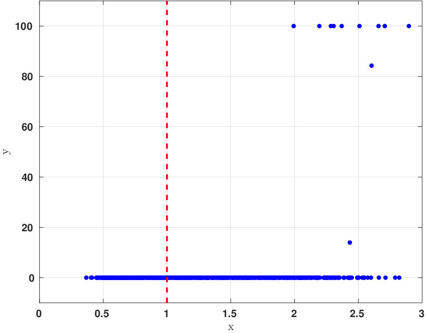
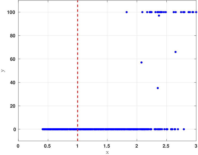
In this experiment, the elements of $\mathbf{x}$ were drawn i.i.d. ${\mathcal{N}}(0,1)$ and the measurements were generated using the AWGN model as discussed above. For each choice of damping factor $\theta_{s}=\theta_{x}$ , scalar stepsize GGAMP was run from the fixed initialization $\{\mathbf{x}^{0}\!=\!\bm{0}$ , ${\mathbf{s}}^{-1}\!=\!\bm{0}$ , $\tau_{x}\!=\!1\}$ and the MSE after $5000$ iterations was recorded. This experiment was then repeated for $100$ realizations of $\{\mathbf{A},\mathbf{x},\mathbf{w}\}$ . The damping factors $\theta_{s}=\theta_{x}$ were varied from $0.7$ to $1$ in steps of $0.005$ . To test the validity of Theorem 2, we present the results in term of the “excess MSE,” defined as the ratio of the MSE achieved by GAMP to the MMSE, which was computed in closed form. To enhance the readability of the plots, the excess MSE was clipped at $100$ dB.

Figures 1 and 2 show the excess MSE versus $\kappa_{\max}(\theta_{s},\theta_{x})$ , which—according to Theorem 2—is the maximum allowed value of $\kappa(\mathbf{A})$ under which GGAMP will converge with damping factors $(\theta_{s},\theta_{x})$ , as defined in (27). In both figures, the dimensions of $\mathbf{A}$ were $200\times 100$ , and the excess MSE from each realization is plotted as a dot. The figures show that the excess MSE was zero dB whenever $\kappa_{\max}(\theta_{s},\theta_{x})>\kappa(\mathbf{A})$ , and conversely the excess MSE was greater than zero dB whenever $\kappa_{\max}(\theta_{s},\theta_{x})<\kappa(\mathbf{A})$ , which verifies the claim of Theorem 2.

Refer to caption — Fig. 1: The excess MSE of GGAMP vs $\kappa_{\max}(\theta_{s},\theta_{x})$ for $\kappa(\mathbf{A})=4$ . Each point represents one realization, and excess MSE values were clipped at $100$ dB. To the right of the red dashed line, the condition $\kappa_{\max}(\theta_{s},\theta_{x})>\kappa(\mathbf{A})$ is satisfied, in which case GGAMP converges to the MMSE solution, as predicted by Theorem 2.

VI-B Local Convergence of GAMP

To test the local stability of damped GAMP, we used the following procedure. For each realization of $\{\mathbf{A},\mathbf{x},\mathbf{y}\}$ , the parameters $\{{\color[rgb]{0,0,0}\bm{\nu}}_{p},\bm{{\color[rgb]{0,0,0}\tau}}_{r},\theta_{s},\theta_{x}\}$ were chosen and vector-stepsize GAMP was run from the initialization $\{\mathbf{x}^{0}=\bm{0}$ , ${\mathbf{s}}^{-1}=\bm{0}$ , $\bm{{\color[rgb]{0,0,0}\tau}}_{x}=\bm{1}\}$ with the stepsizes fixed at the chosen $\{{\color[rgb]{0,0,0}\bm{\nu}}_{p},\bm{{\color[rgb]{0,0,0}\tau}}_{r}\}$ . The values of $\{{\color[rgb]{0,0,0}\bm{\nu}}_{p},\bm{{\color[rgb]{0,0,0}\tau}}_{r},\theta_{s},\theta_{x}\}$ were chosen so that GAMP converged to some fixed point $\{\mathbf{x},{\mathbf{s}},{\mathbf{p}},\mathbf{r}\}$ ; more details are provided below. Next, GAMP was initialized near to the fixed point and tested for local convergence (under the same fixed stepsizes $\{{\color[rgb]{0,0,0}\bm{\nu}}_{p},\bm{{\color[rgb]{0,0,0}\tau}}_{r}\}$ .) In particular, it was initialized at $\{\mathbf{x}^{0}=\mathbf{x}+\mathbf{x}_{\varepsilon}$ , ${\mathbf{s}}^{-1}={\mathbf{s}}\}$ , where the elements of $\mathbf{x}_{\varepsilon}$ were drawn i.i.d. ${\mathcal{N}}(0,1)$ , with $\mathbf{x}_{\varepsilon}$ subsequently normalized such that the initial MSE was $15$ dB above the MSE at the fixed point. This test was repeated $20$ times for each fixed point. If $\theta_{s}\theta_{x}\|\widetilde{\mathbf{A}}\|_{2}^{2}<1$ then, according to Theorem 3, GAMP should converge to the fixed point. Each dot in Figures 3-6 represents the excess MSE, now defined as the ratio of the maximum MSE among all local runs of GAMP to the MSE at the fixed point. The above procedure was repeated for a range of $\theta_{s}=\theta_{x}$ and many realizations of $\{\mathbf{A},\mathbf{x},\mathbf{y}\}$ , as detailed below. As before, the excess MSE values were clipped at $100$ dB before plotting.

Figures 3 and 4 show the excess MSE versus $\theta_{s}\theta_{x}\|\widetilde{\mathbf{A}}\|_{2}^{2}$ for Bernoulli-Gaussian $\mathbf{x}$ with sparsity rate 0.1 and AWGN measurements. Figure 3 investigates the case where $\kappa(\mathbf{A})=4$ and Figure 4 investigates the case where $\kappa(\mathbf{A})=10$ . For each plot, the dimensions of $\mathbf{A}$ were $200\times 100$ , the stepsizes were $\nu_{p_{i}}=(\sum_{j=1}^{n}A_{ij}^{2})^{-1}~\forall i$ , the damping factors $\theta_{s}=\theta_{x}$ were varied from $0.45$ to $0.95$ in steps of $0.05$ , and $50$ realizations of $\{\mathbf{A},\mathbf{x},\mathbf{y}\}$ were tested. Also, $\tau_{r_{j}}=(\sum_{i=1}^{m}A_{ij}^{2})^{-1}$ in Figure 3 and $\tau_{r_{j}}=(10\sum_{i=1}^{m}A_{ij}^{2})^{-1}$ in Figure 4, for all $j$ . This particular choice of $\bm{{\color[rgb]{0,0,0}\tau}}_{r}$ was used to ensure that the fixed-stepsized GAMP converged to a fixed point for the chosen range of $\theta_{s},\theta_{x}$ .

Figure 5 and 6 show the excess MSE versus $\theta_{s}\theta_{x}\|\widetilde{\mathbf{A}}\|_{2}^{2}$ for Bernoulli-Gaussian $\mathbf{x}$ with sparsity rate 0.1 and binary measurements. Figure 5 investigates the case where $\kappa(\mathbf{A})=4$ and Figure 6 investigates the case where $\kappa(\mathbf{A})=10$ . For each plot, the dimensions of $\mathbf{A}$ were $400\times 100$ , the stepsizes were $\nu_{p_{i}}=10~\forall i$ and $\tau_{r_{j}}=1~\forall j$ , the damping factors $\theta_{s}=\theta_{x}$ were varied from $0.45$ to $0.95$ in steps of $0.05$ , and $50$ realizations of $\{\mathbf{A},\mathbf{x},\mathbf{y}\}$ were tested.

Figures 3-6 show an excess MSE of $\approx 0$ dB whenever $\theta_{s}\theta_{x}\|\widetilde{\mathbf{A}}\|_{2}^{2}<1$ , hence verifying Theorem 3.

Conclusions

A key outstanding issue for the adoption of AMP-related methods is their convergence for generic finite-dimensional linear transforms. Similar to other loopy BP-based methods, standard forms of AMP may diverge. In this paper, we presented a damped version of the generalized AMP algorithm that, when used with fixed stepsizes, can guarantee global convergence for Gaussian distributions and local convergence for the minimization of strictly convex functions (i.e., strictly concave log-priors). The required amount of damping is related to the peak-to-average ratio of the squared singular values of the transform matrix. However, much remains unanswered: Most importantly, we have yet to derive a condition for global convergence even in the case of strictly convex functions. Secondly, our analysis assumes the use of fixed stepsizes. Third, short of computing the peak-to-average singular-value ratio, we proposed no method to compute the damping constants. Hence, an adaptive method may be useful in practice. One such method, [23], has been proposed, but it comes without convergence guarantees. Thus, future work might aim to analyze the convergence of such methods. Also, a more recent algorithm, Vector AMP (VAMP) [45, 46], has improved convergence on larger classes of random matrices. Another line of future work could seek conditions for convergence of VAMP on deterministic matrices.

Appendix A Proof of Theorem 1

The variance updates of both Algorithms 1 and 2 are both of the form (19) with different choices of $\mathbf{S}$ . So, the theorem will be proven by showing that the updates (19) converge for any non-negative matrix $\mathbf{S}\geq 0$ . To this end, we use the results in [47]. Specifically, for any ${\color[rgb]{0,0,0}\bm{\nu}}_{w}$ and $\bm{{\color[rgb]{0,0,0}\tau}}_{0}>0$ , define the functions

	$\displaystyle\Phi_{s}(\bm{{\color[rgb]{0,0,0}\tau}}_{x})$	$\displaystyle:=$	$\displaystyle\left[\mathbf{S}\bm{{\color[rgb]{0,0,0}\tau}}_{x}+1./{\color[rgb]{0,0,0}\bm{\nu}}_{w}\right]^{-1}$
	$\displaystyle\Phi_{x}({\color[rgb]{0,0,0}\bm{\nu}}_{s})$	$\displaystyle:=$	$\displaystyle\left[\mathbf{S}^{\text{\sf T}}{\color[rgb]{0,0,0}\bm{\nu}}_{s}+1./\bm{{\color[rgb]{0,0,0}\tau}}_{0}\right]^{-1}$

so that the updates (19) can be written as

{\color[rgb]{0,0,0}\bm{\nu}}_{s}^{t}=\Phi_{s}(\bm{{\color[rgb]{0,0,0}\tau}}_{x}^{t}),\quad\bm{{\color[rgb]{0,0,0}\tau}}_{x}^{t\!+\!1}=\Phi_{x}({\color[rgb]{0,0,0}\bm{\nu}}^{t}_{s}).

It is easy to check that, for any $\mathbf{S}\geq 0$ ,

(i)

$\Phi_{s}(\bm{{\color[rgb]{0,0,0}\tau}}_{x})>0$ ,
(ii)

$\bm{{\color[rgb]{0,0,0}\tau}}_{x}\geq\bm{{\color[rgb]{0,0,0}\tau}}_{x}^{\prime}\Rightarrow\Phi_{s}(\bm{{\color[rgb]{0,0,0}\tau}}_{x})\leq\Phi_{s}(\bm{{\color[rgb]{0,0,0}\tau}}_{x}^{\prime})$ , and
(iii)

For all $\alpha>1$ , $\Phi_{s}(\alpha\bm{{\color[rgb]{0,0,0}\tau}}_{x})>(1/\alpha)\Phi_{s}(\bm{{\color[rgb]{0,0,0}\tau}}_{x})$ .

with the analogous properties being satisfied by $\Phi_{x}({\color[rgb]{0,0,0}\bm{\nu}}_{s})$ . Now let $\Phi:=\Phi_{x}\circ\Phi_{s}$ be the composition of the two functions so that $\bm{{\color[rgb]{0,0,0}\tau}}^{t\!+\!1}_{x}=\Phi(\bm{{\color[rgb]{0,0,0}\tau}}^{t}_{x})$ . Then, $\Phi$ satisfies the three properties:

(i)

$\Phi(\bm{{\color[rgb]{0,0,0}\tau}}_{x})>0$ ,
(ii)

$\bm{{\color[rgb]{0,0,0}\tau}}_{x}\geq\bm{{\color[rgb]{0,0,0}\tau}}_{x}^{\prime}\Rightarrow\Phi(\bm{{\color[rgb]{0,0,0}\tau}}_{x})\geq\Phi(\bm{{\color[rgb]{0,0,0}\tau}}_{x}^{\prime})$ , and
(iii)

For all $\alpha>1$ , $\Phi(\alpha\bm{{\color[rgb]{0,0,0}\tau}}_{x})<\alpha\Phi(\bm{{\color[rgb]{0,0,0}\tau}}_{x})$ .

Also, for any ${\color[rgb]{0,0,0}\bm{\nu}}_{s}\geq 0$ , we have $\Phi_{x}({\color[rgb]{0,0,0}\bm{\nu}}_{s})\leq\bm{{\color[rgb]{0,0,0}\tau}}_{0}$ and therefore, $\Phi(\bm{{\color[rgb]{0,0,0}\tau}}_{x})\leq\bm{{\color[rgb]{0,0,0}\tau}}_{0}$ for all $\bm{{\color[rgb]{0,0,0}\tau}}_{x}\geq 0$ . Hence, taking any $\bm{{\color[rgb]{0,0,0}\tau}}_{x}\geq\bm{{\color[rgb]{0,0,0}\tau}}_{0}$ , we obtain:

\bm{{\color[rgb]{0,0,0}\tau}}_{x}\geq\Phi(\bm{{\color[rgb]{0,0,0}\tau}}_{x}).

Using Theorem 2 in [47], it can be shown that the updates $\bm{{\color[rgb]{0,0,0}\tau}}^{t\!+\!1}_{x}=\Phi(\bm{{\color[rgb]{0,0,0}\tau}}_{x}^{t})$ converge to a unique fixed point. A similar argument shows that ${\color[rgb]{0,0,0}\bm{\nu}}_{s}^{t}$ also converges to a unique fixed point.

Appendix B Linear System Stability Condition

The proofs of both Theorems 2 and 3 are based on analyzing the GAMP algorithm via an equivalent linear system and then applying results from linear stability theory. For both results we will show that the condition of the theorem is equivalent to an eigenvalue test on a certain matrix.

First consider the Gaussian GAMP algorithm with fixed vector stepsizes. With fixed stepsizes and Gaussian estimation functions (17), Algorithm 1 reduces to a linear system:


$\displaystyle{\mathbf{s}}^{t}$	$\displaystyle=$	$\displaystyle(1-\theta_{s}){\mathbf{s}}^{t\!-\!1}+\theta_{s}\mathbf{Q}_{s}({\mathbf{s}}^{t\!-\!1}+{\color[rgb]{0,0,0}\bm{\nu}}_{p}.\mathbf{A}\mathbf{x}^{t})$	(45a)
		$\displaystyle\mbox{}-\theta_{s}{\color[rgb]{0,0,0}\bm{\nu}}_{w}.\mathbf{y}$	(45a)
$\displaystyle\mathbf{x}^{t\!+\!1}$	$\displaystyle=$	$\displaystyle(1-\theta_{x})\mathbf{x}^{t}+\theta_{x}\mathbf{Q}_{x}(\mathbf{x}^{t}-\bm{{\color[rgb]{0,0,0}\tau}}_{r}.\mathbf{A}^{\text{\sf H}}{\mathbf{s}}^{t}-\mathbf{x}_{0})$	(45b)
		$\displaystyle\mbox{}+\theta_{x}\mathbf{x}_{0},$	(45b)

where


$\displaystyle\mathbf{Q}_{s}$	$\displaystyle=$	$\displaystyle\mathop{\mathrm{Diag}}(\mathbf{q}_{s}),\quad\mathbf{q}_{s}={\color[rgb]{0,0,0}\bm{\nu}}_{w}./({\color[rgb]{0,0,0}\bm{\nu}}_{w}+{\color[rgb]{0,0,0}\bm{\nu}}_{p}),$	(46a)
$\displaystyle\mathbf{Q}_{x}$	$\displaystyle=$	$\displaystyle\mathop{\mathrm{Diag}}(\mathbf{q}_{x}),\quad\mathbf{q}_{x}=\bm{{\color[rgb]{0,0,0}\tau}}_{0}./(\bm{{\color[rgb]{0,0,0}\tau}}_{0}+\bm{{\color[rgb]{0,0,0}\tau}}_{r}).$	(46b)

Note that the components of $\mathbf{q}_{s}$ and $\mathbf{q}_{x}$ are in $(0,1)$ . We can write the system (45) in matrix form as

\left[\begin{array}[]{c}{\mathbf{s}}^{t}\\ \mathbf{x}^{t\!+\!1}\end{array}\right]=\mathbf{G}\left[\begin{array}[]{c}{\mathbf{s}}^{t\!-\!1}\\ \mathbf{x}^{t}\end{array}\right]+\mathbf{b},

(47)

for an appropriate matrix $\mathbf{G}$ and vector $\mathbf{b}$ . The matrix $\mathbf{G}$ is given by

\mathbf{G}:=\left[\begin{array}[]{cc}I&0\\ -\theta_{x}\mathop{\mathrm{Diag}}(\bm{{\color[rgb]{0,0,0}\tau}}_{x})\mathbf{A}^{\text{\sf H}}&\mathbf{D}_{x}\end{array}\right]\left[\begin{array}[]{cc}\mathbf{D}_{s}&\theta_{s}\mathop{\mathrm{Diag}}({\color[rgb]{0,0,0}\bm{\nu}}_{s})\mathbf{A}\\ 0&I\end{array}\right],

(48)

where


$\displaystyle\mathbf{D}_{s}$	$\displaystyle=$	$\displaystyle(1-\theta_{s})\mathbf{I}+\theta_{s}\mathbf{Q}_{s}$	(49a)
$\displaystyle\mathbf{D}_{x}$	$\displaystyle=$	$\displaystyle(1-\theta_{x})\mathbf{I}+\theta_{x}\mathbf{Q}_{x}.$	(49b)

Here we have used that

\mathbf{q}_{s}.{\color[rgb]{0,0,0}\bm{\nu}}_{p}={\color[rgb]{0,0,0}\bm{\nu}}_{s},\quad\mathbf{q}_{x}.\bm{{\color[rgb]{0,0,0}\tau}}_{r}=\bm{{\color[rgb]{0,0,0}\tau}}_{x}.

(50)

Note that both $\mathbf{D}_{x}$ and $\mathbf{D}_{s}$ are diagonal matrices with entries in the interval $(0,1)$ .

Now, consider the case of the more general scalar estimation functions satisfying (37) and other assumptions in Section V. Due to the differentiability assumptions, to prove the local stability, we only have to look at the linearization of the system around the fixed points [44]. With fixed stepsizes, the linearization of the updates in Algorithm 1 around any fixed point is given by


$\displaystyle{\mathbf{s}}^{t}$	$\displaystyle=$	$\displaystyle(1-\theta_{s}){\mathbf{s}}^{t\!-\!1}+\theta_{s}\mathbf{Q}_{s}({\mathbf{s}}^{t\!-\!1}+{\color[rgb]{0,0,0}\bm{\nu}}_{p}.\mathbf{A}\mathbf{x}^{t})$	(51a)
$\displaystyle\mathbf{x}^{t\!+\!1}$	$\displaystyle=$	$\displaystyle(1-\theta_{x})\mathbf{x}^{t}+\theta_{x}\mathbf{Q}_{x}(\mathbf{x}^{t}-\bm{{\color[rgb]{0,0,0}\tau}}_{r}.\mathbf{A}^{\text{\sf H}}{\mathbf{s}}^{t})$	(51b)

where the matrices $\mathbf{Q}_{s}$ and $\mathbf{Q}_{x}$ in (46) are replaced by the derivatives (38). This linear system is also of the form (47) with the same matrix (48). Also, under the assumptions of the theorem, $\mathbf{q}_{s}$ and $\mathbf{q}_{x}$ are vectors with components in $(0,1)$ .

Hence, we conclude that to prove the global stability of Gaussian GAMP, or the local stability of GAMP under the assumptions of Theorem 3, it suffices to show that the linear system (47) with a matrix $\mathbf{G}$ of the form (48) is stable. The matrices $\mathbf{D}_{s}$ and $\mathbf{D}_{x}$ are given in (49) where $\mathbf{Q}_{s}$ and $\mathbf{Q}_{x}$ are diagonal matrices with elements in $(0,1)$ .

To evaluate this condition, first recall that the linear system (47) is stable when the eigenvalues of $\mathbf{G}$ are in the unit circle. However, if we define

\mathbf{T}=\left[\begin{array}[]{cc}\mathop{\mathrm{Diag}}^{-1/2}(\theta_{s}{\color[rgb]{0,0,0}\bm{\nu}}_{s})&0\\ 0&\mathop{\mathrm{Diag}}^{-1/2}(\theta_{x}\bm{{\color[rgb]{0,0,0}\tau}}_{x})\end{array}\right],

the eigenvalues of $\mathbf{G}$ are identical to those of $\mathbf{H}$ given by

\mathbf{H}:=\mathbf{T}\mathbf{G}\mathbf{T}^{-1}=\left[\begin{array}[]{cc}\mathbf{I}&0\\ -\mathbf{F}^{\text{\sf H}}&\mathbf{D}_{x}\end{array}\right]\left[\begin{array}[]{cc}\mathbf{D}_{s}&\mathbf{F}\\ 0&\mathbf{I}\end{array}\right],

(52)

where

\mathbf{F}=\sqrt{\theta_{s}\theta_{x}}\mathop{\mathrm{Diag}}({\color[rgb]{0,0,0}\bm{\nu}}_{s}^{1/2})\mathbf{A}\mathop{\mathrm{Diag}}(\bm{{\color[rgb]{0,0,0}\tau}}_{x}^{1/2}).

(53)

Expanding the matrix product in (52), we get

\mathbf{H}=\left[\begin{array}[]{cc}\mathbf{D}_{s}&\mathbf{F}\\ -\mathbf{F}^{\text{\sf H}}\mathbf{D}_{s}&\mathbf{D}_{x}-\mathbf{F}^{\text{\sf H}}\mathbf{F}\end{array}\right].

(54)

Now, for any $\lambda\in{\mathbb{C}}$ , define the matrix

\mathbf{H}_{\lambda}:=\lambda\mathbf{I}-\mathbf{H}=\left[\begin{array}[]{cc}\lambda\mathbf{I}-\mathbf{D}_{s}&-\mathbf{F}\\ \mathbf{F}^{\text{\sf H}}\mathbf{D}_{s}&\lambda\mathbf{I}-\mathbf{D}_{x}+\mathbf{F}^{\text{\sf H}}\mathbf{F}\end{array}\right].

(55)

For stability, we need to show that for any $|\lambda|\geq 1$ , $\mathbf{H}_{\lambda}$ is invertible. We simplify this condition as follows: Consider any $\lambda$ with $|\lambda|\geq 1$ . Now, $\mathbf{D}_{s}$ in (49b) is a diagonal matrix with entries in $[0,1)$ . Hence $\lambda\mathbf{I}-\mathbf{D}_{s}$ is invertible since $|\lambda|\geq 1$ . Therefore, taking a Schur complement, we see that $\mathbf{H}_{\lambda}$ is invertible if and only if the matrix

	$\displaystyle\mathbf{J}_{\lambda}$	$\displaystyle:=$	$\displaystyle\lambda\mathbf{I}-\mathbf{D}_{x}+\mathbf{F}^{\text{\sf H}}\mathbf{F}+\mathbf{F}^{\text{\sf H}}\mathbf{D}_{s}(\lambda\mathbf{I}-\mathbf{D}_{s})^{-1}\mathbf{F}$
		$\displaystyle=$	$\displaystyle\lambda\mathbf{I}-\mathbf{D}_{x}+\lambda\mathbf{F}^{\text{\sf H}}(\lambda\mathbf{I}-\mathbf{D}_{s})^{-1}\mathbf{F}.$

is invertible. We can summarize the result as follows.

Lemma 1

Consider the GAMP Algorithm 1 for any scalar estimation functions satisfying the conditions in Section V including (37). The GAMP algorithm is locally stable around a fixed point if and only if $\mathbf{J}_{\lambda}$ is invertible for all $|\lambda|\geq 1$ , where

\mathbf{J}_{\lambda}=\lambda\mathbf{I}-\mathbf{D}_{x}+\lambda\mathbf{F}^{\text{\sf H}}(\lambda\mathbf{I}-\mathbf{D}_{s})^{-1}\mathbf{F},

(56)

and $\mathbf{F}$ is given in (53). In the special case of Gaussian estimation functions (17), the above condition implies the GAMP Algorithm 1, will be globally stable.

A similar calculation can be performed for the GAMP algorithm with scalar stepsizes. In this case, the vector stepsizes such as $\bm{{\color[rgb]{0,0,0}\tau}}_{x}$ and ${\color[rgb]{0,0,0}\bm{\nu}}_{s}$ are replaced with the scalar quantities $\tau_{x}$ and $\nu_{s}$ . For the case of Gaussian estimation functions (17) and identical variances (20) we obtain the following:

Lemma 2

Consider the GAMP Algorithm 2 with scalar stepsizes, Gaussian scalar estimation functions (17) and identical variances (20). Then, the algorithm is globally stable if and only if $\mathbf{J}_{\lambda}$ is invertible for all $|\lambda|\geq 1$ , where

\mathbf{J}_{\lambda}=(\lambda-d_{x})\mathbf{I}+\frac{\lambda}{\lambda-d_{s}}\mathbf{F}^{\text{\sf H}}\mathbf{F},

(57)

where

\mathbf{F}=\sqrt{\theta_{s}\theta_{x}\nu_{s}\tau_{x}}\mathbf{A},

(58)

and


$\displaystyle d_{s}$	$\displaystyle=$	$\displaystyle(1-\theta_{s})+\theta_{s}q_{s},\quad q_{s}=\frac{\nu_{w}}{\nu_{p}+\nu_{w}},$	(59a)
$\displaystyle d_{x}$	$\displaystyle=$	$\displaystyle(1-\theta_{x})+\theta_{x}q_{x},\quad q_{x}=\frac{\tau_{0}}{\tau_{0}+\tau_{r}}.$	(59b)

Appendix C Proof of Theorem 2

Our first step in the proof is to simplify the condition in Lemma 2.

Lemma 3

Consider the GAMP algorithm with scalar stepsizes, Algorithm 2, with the Gaussian scalar estimation functions (17) and fixed stepsizes. Then the system is stable if and only if

\sigma^{2}_{\max}(\mathbf{A})<\|\mathbf{A}\|^{2}_{F}\gamma,

(60)

where

\gamma:=\frac{1}{\|\mathbf{A}\|^{2}_{F}\theta_{s}\theta_{x}}\left[\frac{2}{\tau_{x}}-\frac{\theta_{x}}{\tau_{0}}\right]\left[\frac{2}{\nu_{s}}-\frac{\theta_{s}}{\nu_{w}}\right].

(61)

Proof:

From Lemma 2, we know that the system is stable if and only if $\mathbf{J}_{\lambda}$ in (57) is invertible for all $|\lambda|\geq 1$ . To evaluate this condition, suppose that $\mathbf{J}_{\lambda}$ is not invertible for some $|\lambda|\geq 1$ . Then, there exists an $\mathbf{v}\neq 0$ such that $\mathbf{J}_{\lambda}\mathbf{v}=0$ , which implies that

\mathbf{F}^{\text{\sf H}}\mathbf{F}\mathbf{v}=\frac{(d_{x}-\lambda)(\lambda-d_{s})}{\lambda}\mathbf{v}.

Using the expression for $\mathbf{F}$ in (58), this is equivalent to

\mathbf{A}^{\text{\sf H}}\mathbf{A}\mathbf{v}=\frac{(d_{x}-\lambda)(\lambda-d_{s})}{\theta_{x}\theta_{s}\tau_{x}\nu_{s}\lambda}\mathbf{v}.

Thus, $\mathbf{v}$ is an eigenvector of $\mathbf{A}^{\text{\sf H}}\mathbf{A}$ . But, $\sigma^{2}$ is an eigenvalue of $\mathbf{A}^{\text{\sf H}}\mathbf{A}$ if and only if $\sigma$ is a singular value of $\mathbf{A}$ . Hence, we conclude that $\mathbf{J}_{\lambda}$ is non-invertible if and only if there exists a singular value $\sigma$ of $\mathbf{A}$ such that

\sigma^{2}\theta_{x}\theta_{z}\tau_{x}\nu_{s}\lambda=(d_{x}-\lambda)(\lambda-d_{s}).

Equivalently, we have shown that the system is stable if and only if the the second-order polynomial

p(\lambda):=\lambda^{2}+(\sigma^{2}\theta_{x}\theta_{s}\tau_{x}\nu_{s}-d_{x}-d_{s})\lambda+d_{s}d_{x}

has stable roots for all singular values of $\mathbf{A}$ , $\sigma$ . Now recall that $d_{s}$ and $d_{x}\in(0,1)$ . By the Jury stability condition, the $p(\lambda)$ has stable roots if and only $p(1)>0$ and $p(-1)>0$ . Now, the first condition is always satisfied since

p(1)=\sigma^{2}\theta_{x}\theta_{z}\tau_{x}\nu_{s}+(1-d_{s})(1-d_{x})>0.

So, the polynomial is stable if and only if

0<p(-1)=-\sigma^{2}\theta_{x}\theta_{z}\tau_{x}\nu_{s}+(1+d_{s})(1+d_{x}),

or equivalently,

\sigma^{2}\theta_{x}\theta_{z}\tau_{x}\nu_{s}<(1+d_{s})(1+d_{x}).

For this to be true for all singular values of $\mathbf{A}$ , we need

\sigma_{\max}^{2}(\mathbf{A})\theta_{x}\theta_{z}\tau_{x}\nu_{s}<(1+d_{s})(1+d_{x}).

Thus, the system is stable if and only if (60) is satisfied with

\gamma:=\frac{(1+d_{x})(1+d_{s})}{\theta_{s}\theta_{x}\nu_{s}\tau_{x}\|\mathbf{A}\|^{2}_{F}}.

(62)

So, we simply need to prove that (62) matches the definition in (61). To this end, first note that

\frac{1+d_{x}}{\tau_{x}}\stackrel{{\scriptstyle(a)}}{{=}}\frac{2-\theta_{x}}{\tau_{x}}+\frac{\theta_{x}}{\tau_{r}}\stackrel{{\scriptstyle(b)}}{{=}}\frac{2}{\tau_{x}}-\frac{\theta_{x}}{\tau_{0}},

(63)

where (a) follows from the definition $q_{x}=\tau_{x}/\tau_{r}$ in (49a) and (b) follows from the fixed-point equation (22b). Similarly using (49b) and (22a), we obtain that

\frac{1+d_{s}}{\nu_{s}}=\frac{2-\theta_{s}}{\nu_{s}}+\frac{\theta_{s}}{\nu_{p}}=\frac{2}{\nu_{s}}-\frac{\theta_{s}}{\nu_{w}}.

(64)

Substituting (63) and (64) into (62), we obtain (61) and the lemma is proven. $\Box$

Let

\Gamma:=\inf_{\nu_{w}>0}\gamma,

(65)

where $\gamma$ is defined in (61) and the minimization is over $\nu_{w}$ with the other parameters, $\|\mathbf{A}\|^{2}_{F}$ , $\tau_{0}$ , $m$ and $n$ , being fixed. It follows that if

\sigma^{2}(\mathbf{A})<\Gamma\|\mathbf{A}\|^{2}_{F}

then the system is stable for all $\nu_{w}$ . Conversely, if

\sigma^{2}(\mathbf{A})>\Gamma\|\mathbf{A}\|^{2}_{F}

then there exists at least one $\nu_{w}$ such that the system is unstable. So, the theorem will be proven if we can show that $\Gamma$ defined in (65) matches the expression in (23).

To calculate the minima in (65), it is useful to write a scaled version of the updates. Let


$\displaystyle s$	$\displaystyle:=\frac{m}{\\|\mathbf{A}\\|^{2}_{F}\nu_{s}\tau_{0}},\quad x:=\frac{\tau_{0}}{\tau_{x}}$	(66a)
$\displaystyle u$	$\displaystyle:=\frac{m}{\\|\mathbf{A}\\|^{2}_{F}\nu_{w}\tau_{0}},\quad\beta:=\frac{m}{n}.$	(66b)

Then, the fixed points of (22) are given by

s=\frac{1}{x}+u,\quad x=\frac{\beta}{s}+1.

(67)

Also, $\gamma$ in (61) is given by,

\gamma=\frac{1}{m\theta_{s}\theta_{x}}(2x-\theta_{x})(2s-\theta_{s}u).

(68)

Moreover, the minimization in (65) is equivalent to

\Gamma=\inf_{u\geq 0}\gamma,

(69)

since minimizing over $\nu_{w}$ is equivalent to minimizing over $u$ in the scaled system. To evaluate the minima (69), we first prove the following.

Lemma 4

The minimization in (69) is given by

\Gamma=\lim_{u\rightarrow 0}\gamma.

(70)

That is, the minima is achieved as $u\rightarrow 0$ .

Proof:

From (67),

\frac{u\beta}{s}=s-u+\beta-1.

(71)

Substituting (67) into (68) and applying (71), we obtain

$\displaystyle\gamma$	$\displaystyle=\frac{1}{m\theta_{s}\theta_{x}}\left(\frac{2\beta}{s}+2-\theta_{x}\right)(2s-\theta_{s}u)$
	$\displaystyle=\frac{1}{m\theta_{s}\theta_{x}}\left[4\beta-(2-\theta_{x})\theta_{s}u+2(2-\theta_{x})s-\frac{2\beta\theta_{s}u}{s}\right]$
	$\displaystyle=\frac{1}{m\theta_{s}\theta_{x}}\left[A(s,u)+B\right],$	(72)

where

\displaystyle\begin{split}A(s,u)&:=2(2-\theta_{x}-\theta_{s})s+\theta_{x}\theta_{s}u\\ B&:=4\beta-2\theta_{s}(\beta-1)\end{split}

(73)

Now let $s^{\prime}$ , $x^{\prime}$ and $A^{\prime}(s,u)$ denote the derivatives with respect to $u$ . From (67) we have

s^{\prime}=-\frac{x^{\prime}}{x^{2}}+1,\quad x^{\prime}=-\frac{\beta s^{\prime}}{s^{2}},

(74)

and therefore,

s^{\prime}=\frac{s^{2}x^{2}}{s^{2}x^{2}-\beta}.

(75)

Now from (67), we have

sx>1\mbox{ and }sx>\beta.

Therefore, $(sx)^{2}>\beta$ and hence, from (75), $s^{\prime}>0$ . It follows that

A^{\prime}(s,u)=2(2-\theta_{x}-\theta_{s})s^{\prime}+\theta_{x}\theta_{s}>0,

since both $2-\theta_{x}-\theta_{s}\geq 0$ and $\theta_{x}\theta_{x}>0$ . Hence, from (72), we have

\frac{\partial\gamma}{\partial u}=\frac{A^{\prime}(s,u)}{m\theta_{s}\theta_{x}}>0,

and it follows that the $\gamma$ is minimized by taking $u$ as small as possible. Therefore,

\Gamma=\inf_{u\geq 0}\gamma=\lim_{u\rightarrow 0}\gamma.

$\Box$

We conclude by evaluating the limit in (70). The following lemma shows that value of the minimization agrees with (23), and hence completes the proof of the theorem.

Lemma 5

For any damping constants $\theta_{s}$ , $\theta_{x}$ , the limit in (70) is given by (23).

Proof:

First consider the case when $\beta\geq 1$ (i.e. $m\geq n$ ). In this case, as $u\rightarrow 0$ the solutions to the fixed points (67) will satisfy $s\rightarrow 0$ and $x\rightarrow\infty$ . Hence, the limit of $A(s,u)$ in (73) is

\lim_{u\rightarrow 0}A(s,u)=0.

Therefore,

	$\displaystyle\Gamma$	$\displaystyle=\lim_{u\rightarrow 0}\gamma\stackrel{{\scriptstyle(a)}}{{=}}\frac{B}{m\theta_{s}\theta_{x}}\stackrel{{\scriptstyle(b)}}{{=}}\frac{4\beta-2\theta_{s}(\beta-1)}{m\theta_{s}\theta_{x}}$
		$\displaystyle\stackrel{{\scriptstyle(c)}}{{=}}\frac{2\left[(2-\theta_{s})m+\theta_{s}n\right]}{\theta_{s}\theta_{x}mn},$

where (a) used (72); (b) used (73) and (c) used the fact that $\beta=m/n$ . This proves the $m\geq n$ case of (23).

For the case when $\beta<1$ (i.e. $m<n$ ) and $u=0$ , the solutions to fixed point in (67) are

x=\frac{1}{1-\beta},\quad s=\frac{1}{x}=1-\beta.

Substituting $s=1-\beta$ and $u=0$ into (72),

	$\displaystyle\gamma$	$\displaystyle=\frac{1}{m\theta_{s}\theta_{x}}\left[2(2-\theta_{x}-\theta_{s})(1-\beta)+4\beta-2\theta_{s}(\beta-1)\right]$
		$\displaystyle=\frac{2\left[(2-\theta_{x})n+\theta_{x}m\right]}{\theta_{s}\theta_{x}mn},$

where again we have used the fact that $\beta=m/n$ . Therefore,

\Gamma=\lim_{u\rightarrow 0}\gamma=\frac{2\left[(2-\theta_{x})n+\theta_{x}m\right]}{\theta_{s}\theta_{x}mn},

and this proves the $m<n$ case of (23). $\Box$

Appendix D Proof of Theorem 3

We begin with a technical lemma.

Lemma 6

Let $\lambda\in{\mathbb{C}}$ , $d_{s,\max},d_{x},\sigma\in[0,1)$ with $|\lambda|\geq 1$ . Define the set,

P:=\left\{\lambda-d_{x}+\frac{\sigma^{2}\lambda}{\lambda-d_{s}}~\mid~d_{s}\in[0,d_{s,\max}]~\right\}.

(76)

Then $0\not\in\mbox{conv}(P)$ , the convex hull of $P$ .

Proof:

Write $\lambda$ in polar coordinates, $\lambda=re^{i\theta}$ . We first consider the case where $\theta\in(0,\pi)$ . Under this assumption, we claim for all $z\in P$ ,

\mbox{Imag}((\bar{\lambda}-d_{x})z)<0.

(77)

Since $P$ is compact, this would imply that (77) holds for all $z\in\mbox{conv}(P)$ . In particular, $0\not\in\mbox{conv}(P)$ . So, we need to show that (77) holds for all $z\in P$ .

To this end, let $z\in P$ so that,

z=\lambda-d_{x}+\frac{\sigma^{2}\lambda}{\lambda-d_{s}},

(78)

for some $d_{s}\in[0,d_{s,\max}]$ . Then,

		$\displaystyle\mbox{Imag}((\bar{\lambda}-d_{x})z)$
		$\displaystyle=\mbox{Imag}\left[\|\lambda-d_{x}\|^{2}+\frac{\sigma^{2}(\bar{\lambda}-d_{x})\lambda}{\lambda-d_{s}}\right]$
		$\displaystyle=\frac{\sigma^{2}}{\|\lambda-d_{s}\|^{2}}\mbox{Imag}\left[(\bar{\lambda}-d_{x})(\bar{\lambda}-d_{s})\lambda\right]$
		$\displaystyle=\frac{\sigma^{2}}{\|\lambda-d_{s}\|^{2}}\mbox{Imag}\left[r^{2}\bar{\lambda}-(d_{s}+d_{x})\|\lambda\|^{2}+d_{s}d_{x}\lambda\right]$
		$\displaystyle=\frac{\sigma^{2}}{\|\lambda-d_{s}\|^{2}}\left[-r^{3}\sin\theta+rd_{s}d_{x}\sin\theta\right]$
		$\displaystyle=\frac{r\sin\theta\sigma^{2}}{\|\lambda-d_{s}\|^{2}}\left[-r^{2}+d_{s}d_{x}\right].$		(79)

Now, since $\theta\in(0,\pi)$ , $\sin\theta>0$ . Also, since $|\lambda|\geq 1$ , $r\geq 1$ . Therefore, $r^{2}>d_{s}d_{x}$ since $d_{s},d_{x}<1$ . Hence, (79) shows that (77) holds for all $z\in P$ .

Similarly, for the case when $\theta\in(-\pi,0)$ , (79) shows that

\mbox{Imag}((\bar{\lambda}-d_{x})z)>0,

(80)

for all $z\in P$ . The same argument then shows that $0\not\in\mbox{conv}(P)$ .

It remains to consider the cases when $\theta=0$ or $\theta=\pi$ . For $\theta=0$ , $\lambda=r$ and any $z\in P$ is of the form,

z=r-d_{x}+\frac{\sigma^{2}r}{r-d_{s}}\stackrel{{\scriptstyle(a)}}{{>}}r-d_{x}\stackrel{{\scriptstyle(b)}}{{>}}0,

where (a) follows from the fact that $r>d_{s}$ and (b) follows from the fact that $r>d_{x}$ . So, for all $z\in P$ , $z$ is real and positive. Hence, $0\not\in\mbox{conv}(P)$ . Similarly, when $\theta=\pi$ , $\lambda=-r$ and

z=-r-d_{x}+\frac{\sigma^{2}r}{r+d_{s}}<-r-d_{x}+\sigma^{2}\stackrel{{\scriptstyle(a)}}{{<}}-r+\sigma^{2}\stackrel{{\scriptstyle(b)}}{{<}}0,

where (a) follows since $d_{x}>0$ and (b) follows since $r\geq 1$ and $\sigma^{2}<1$ . Therefore, for all $z\in P$ , $z$ is real and negative. Hence, $0\not\in\mbox{conv}(P)$ . We have thus shown that $0\not\in\mbox{conv}(P)$ for all values of $\theta$ . $\Box$

We can now prove the main result. Suppose that (43) is satisfied. By the definition of $\mathbf{F}$ in (53) and $\widetilde{\mathbf{A}}$ in (39), we have that

\sigma^{2}_{\max}(\mathbf{F})<1.

(81)

Now, from Lemma 1 we need to show that the matrix $\mathbf{J}_{\lambda}$ in (56) is invertible for all $\lambda\in{\mathbb{C}}$ with $|\lambda|\geq 1$ . We prove this by contradiction.

Suppose that $\mathbf{J}_{\lambda}$ in (56) is not invertible for some $\lambda$ with $|\lambda|\geq 1$ . Then, there exists an $\mathbf{x}$ with $\|\mathbf{x}\|^{2}=1$ such that $\mathbf{x}^{\text{\sf H}}\mathbf{J}_{\lambda}\mathbf{x}=0$ . Therefore, if we define $\mathbf{y}=\mathbf{F}\mathbf{x}$ , the definition of $\mathbf{J}_{\lambda}$ in (56) shows that

\mathbf{x}^{\text{\sf H}}(\lambda\mathbf{I}-\mathbf{D})\mathbf{x}+\lambda\mathbf{y}^{\text{\sf H}}(\lambda\mathbf{I}-\mathbf{D}_{s})^{-1}\mathbf{y}=0.

Since $\mathbf{D}_{x}$ and $\mathbf{D}_{s}$ are diagonal, we have

\sum_{j=1}^{n}(\lambda-d_{x_{j}})|x_{j}|^{2}+\sum_{i=1}^{m}\frac{\lambda}{\lambda-d_{s_{j}}}|y_{j}|^{2}=0.

(82)

Since $\|\mathbf{x}\|^{2}=1$ , we have $\sum_{j}|x_{j}|^{2}=1$ . Also, since $\|\mathbf{F}\|_{2}^{2}=\sigma^{2}_{\max}(\mathbf{F})<1$ ,

\sum_{i}|y_{i}|^{2}=\|\mathbf{F}\mathbf{x}\|^{2}=\sigma^{2}\|\mathbf{x}\|^{2}=\sigma^{2}

for some $\sigma^{2}<1$ . Therefore, (82) shows that

0\in\mbox{conv}(P),

(83)

where $P$ is the set (76) where

d_{x}=\sum_{j=1}^{n}d_{x_{j}}|x_{j}|^{2},\quad d_{s,\max}=\max_{j}d_{s_{j}}.

(84)

Now, from (38) and the contractivity assumption (37), the elements of the diagonal matrices $\mathbf{Q}_{x}$ and $\mathbf{Q}_{s}$ must be in the interval $(0,1)$ . Hence, from (49), the elements $d_{x_{j}}$ and $d_{s_{j}}\in(0,1)$ . Therefore, $d_{x},d_{s,\max}$ in (84) are in $(0,1)$ . From Lemma 6, $0\not\in\mbox{conv}(P_{\lambda})$ which is a contradiction of (83). Hence, the assumption that $\mathbf{J}_{\lambda}$ is not invertible must be false, and the theorem is proven.

References

[1] S. Rangan, P. Schniter, and A. K. Fletcher, “On the convergence of approximate message passing with arbitrary matrices,” in Proc. IEEE ISIT, Jul. 2014, pp. 236–240.
[2] A. Chambolle, R. A. DeVore, N. Y. Lee, and B. J. Lucier, “Nonlinear wavelet image processing: Variational problems, compression, and noise removal through wavelet shrinkage,” IEEE Trans. Image Process., vol. 7, no. 3, pp. 319–335, Mar. 1998.
[3] I. Daubechies, M. Defrise, and C. D. Mol, “An iterative thresholding algorithm for linear inverse problems with a sparsity constraint,” Commun. Pure Appl. Math., vol. 57, no. 11, pp. 1413–1457, Nov. 2004.
[4] S. J. Wright, R. D. Nowak, and M. Figueiredo, “Sparse reconstruction by separable approximation,” IEEE Trans. Signal Process., vol. 57, no. 7, pp. 2479–2493, Jul. 2009.
[5] A. Beck and M. Teboulle, “A fast iterative shrinkage-thresholding algorithm for linear inverse problem,” SIAM J. Imag. Sci., vol. 2, no. 1, pp. 183––202, 2009.
[6] Y. E. Nesterov, “Gradient methods for minimizing composite objective function,” center for Operations Research and Econometrics (CORE), Catholic Univ. Louvain, Louvain-la-Neuve, Belgium, CORE Discussion Paper 2007/76, 2007.
[7] J. Bioucas-Dias and M. Figueiredo, “A new TwIST: Two-step iterative shrinkage/thresholding algorithms for image restoration,” IEEE Trans. Image Process., vol. 16, no. 12, pp. 2992 – 3004, Dec. 2007.
[8] S. Boyd, N. Parikh, E. Chu, B. Peleato, and J. Eckstein, “Distributed optimization and statistical learning via the alternating direction method of multipliers,” Found. Trends Mach. Learn., vol. 3, pp. 1–122, 2010.
[9] E. Esser, X. Zhang, and T. F. Chan, “A general framework for a class of first order primal-dual algorithms for convex optimization in imaging science,” SIAM J. Imaging Sci., vol. 3, no. 4, pp. 1015–1046, 2010.
[10] A. Chambolle and T. Pock, “A first-order primal-dual algorithm for convex problems with applications to imaging,” J. Math. Imaging Vis., vol. 40, pp. 120–145, 2011.
[11] B. He and X. Yuan, “Convergence analysis of primal-dual algorithms for a saddle-point problem: From contraction perspective,” SIAM J. Imaging Sci., vol. 5, no. 1, pp. 119–149, 2012.
[12] N. Komodakis and J.-C. Pesquet, “Playing with duality: An overview of recent primal-dual approaches for solving large-scale optimization problems,” IEEE Signal Process. Mag., vol. 32, no. 6, pp. 31–54, 2015.
[13] D. L. Donoho, A. Maleki, and A. Montanari, “Message-passing algorithms for compressed sensing,” Proc. Nat. Acad. Sci., vol. 106, no. 45, pp. 18 914–18 919, Nov. 2009.
[14] ——, “Message passing algorithms for compressed sensing I: Motivation and construction,” in Proc. Info. Theory Workshop, Jan. 2010, pp. 1–5.
[15] S. Rangan, “Generalized approximate message passing for estimation with random linear mixing,” in Proc. IEEE ISIT, 2011, pp. 2174–2178.
[16] M. Bayati and A. Montanari, “The dynamics of message passing on dense graphs, with applications to compressed sensing,” IEEE Trans. Inform. Theory, vol. 57, no. 2, pp. 764–785, Feb. 2011.
[17] A. Javanmard and A. Montanari, “State evolution for general approximate message passing algorithms, with applications to spatial coupling,” Information and Inference, vol. 2, no. 2, pp. 115–144, 2013.
[18] M. Bayati, M. Lelarge, and A. Montanari, “Universality in polytope phase transitions and message passing algorithms,” Ann. Appl. Prob., vol. 25, no. 2, pp. 753–822, 2015.
[19] C. Rush and R. Venkataramanan, “Finite-sample analysis of approximate message passing,” in Proc. IEEE ISIT, 2016, pp. 755–759.
[20] S. Rangan, P. Schniter, E. Riegler, A. Fletcher, and V. Cevher, “Fixed points of generalized approximate message passing with arbitrary matrices,” in Proc. IEEE ISIT, Jul. 2013, pp. 664–668.
[21] F. Krzakala, A. Manoel, E. W. Tramel, and L. Zdeborová, “Variational free energies for compressed sensing,” in Proc. IEEE ISIT, Jul. 2014, pp. 1499–1503.
[22] J. S. Yedidia, W. T. Freeman, and Y. Weiss, “Understanding belief propagation and its generalizations,” in Exploring Artificial Intelligence in the New Millennium. San Francisco, CA: Morgan Kaufmann Publishers, 2003, pp. 239–269.
[23] J. Vila, P. Schniter, S. Rangan, F. Krzakala, and L. Zdeborová, “Adaptive damping and mean removal for the generalized approximate message passing algorithm,” in Proc. IEEE ICASSP, 2015, pp. 2021–2025.
[24] F. Caltagirone, L. Zdeborová, and F. Krzakala, “On convergence of approximate message passing,” in Proc. IEEE ISIT, Jul. 2014, pp. 1812–1816.
[25] M. Pretti, “A message-passing algorithm with damping,” Journal of Statistical Mechanics: Theory and Experiment, vol. 2005, no. 11, p. P11008, 2005.
[26] V. Kolmogorov, “Convergent tree-reweighted message passing for energy minimization,” IEEE Trans. Pattern Analysis and Machine Intelligence, vol. 28, no. 10, pp. 1568–1583, 2006.
[27] A. Globerson and T. S. Jaakkola, “Fixing max-product: Convergent message passing algorithms for map lp-relaxations,” in Proc. NIPS, 2007, pp. 553–560.
[28] A. Manoel, F. Krzakala, E. W. Tramel, and L. Zdeborová, “Swept approximate message passing for sparse estimation,” in Proc. ICML, 2015, pp. 1123–1132.
[29] S. Rangan, A. K. Fletcher, P. Schniter, and U. S. Kamilov, “Inference for generalized linear models via alternating directions and Bethe free energy minimization,” in Proc. IEEE ISIT, 2015, pp. 1640–1644.
[30] D. Bickson, “Gaussian belief propagation: Theory and application,” arXiv:0811.2518, 2008.
[31] D. Dolev, D. Bickson, and J. K. Johnson, “Fixing convergence of Gaussian belief propagation,” in Proc. IEEE ISIT, 2009, pp. 1674–1678.
[32] P. Schniter and S. Rangan, “Compressive phase retrieval via generalized approximate message passing,” in Proc. Allerton Conf. Comm. Control & Comput., Monticello, IL, Oct. 2012.
[33] S. Rangan, “Generalized approximate message passing for estimation with random linear mixing,” arXiv:1010.5141v1 [cs.IT]., Oct. 2010.
[34] P. L. Combettes and V. R. Wajs, “Signal recovery by proximal forward-backward splitting,” Multiscale Model. Simul., vol. 4, pp. 1168–1200, 2005.
[35] K. J. Arrow, L. Hurwicz, and H. Uzawa, Studies in Linear and Non-Linear Programming. Palo Alto, CA: Stanford University Press, 1958.
[36] T. Goldstein, E. Esser, and R. Baraniuk, “Adaptive primal-dual hybrid gradient methods for saddle-point problems,” arXiv:1305.0546, 2013.
[37] V. A. Marčenko and L. A. Pastur, “Distribution of eigenvalues for some sets of random matrices,” Math. USSR–Sbornik, vol. 1, no. 4, pp. 457–483, 1967.
[38] D. M. Malioutov, J. K. Johnson, and A. S. Willsky, “Walk-sums and belief propagation in Gaussian graphical models,” The Journal of Machine Learning Research, vol. 7, pp. 2031–2064, 2006.
[39] Y. Weiss and W. T. Freeman, “Correctness of belief propagation in Gaussian graphical models of arbitrary topology,” in Advances in neural information processing systems, 2000, pp. 673–679.
[40] P. Rusmevichientong and B. Van Roy, “An analysis of belief propagation on the turbo decoding graph with Gaussian densities,” IEEE Trans. Inform. Theory, vol. 47, no. 2, pp. 745–765, 2001.
[41] C. C. Moallemi and B. Van Roy, “Convergence of min-sum message passing for quadratic optimization,” IEEE Trans. Inform. Theory, vol. 55, no. 5, pp. 2413–2423, 2009.
[42] D. M. Malioutov, J. K. Johnson, and A. S. Willsky, “Walk-sums and belief propagation in Gaussian graphical models,” J. Machine Learning Res., vol. 7, pp. 2031–2064, Oct. 2006.
[43] C. C. Moallemi and B. Van Roy, “Convergence of min-sum message-passing for convex optimization,” IEEE Trans. Inform. Theory, vol. 56, no. 4, pp. 2041–2050, 2010.
[44] M. Vidyasagar, Nonlinear Systems Analysis. Englewood Cliffs, NJ: Prentice-Hall, 1978.
[45] S. Rangan, P. Schniter, and A. K. Fletcher, “Vector approximate message passing,” in Proc. IEEE ISIT, 2017, pp. 1588–1592.
[46] A. K. Fletcher and P. Schniter, “Learning and free energies for vector approximate message passing,” in IEEE Intl. Conf. Acoustics, Speech and Signal Processing (ICASSP), 2017, pp. 4247–4251.
[47] R. D. Yates, “A framework for uplink power control in cellular radio systems,” IEEE J. Sel. Areas Comm., vol. 13, no. 7, pp. 1341–1347, September 1995.

$\displaystyle\\|\mathbf{A}\\|^{2}_{2}$	$\displaystyle=$	$\displaystyle\lambda_{\max}(\mathbf{A}^{\text{\sf H}}\mathbf{A})\leq 1+\|1-\lambda_{\max}(\mathbf{A}^{\text{\sf H}}\mathbf{A})\|$
	$\displaystyle=$	$\displaystyle 1+\|\lambda_{\max}(\mathbf{A}^{\text{\sf H}}\mathbf{A}-\mathbf{I})\|\leq 1+\lambda_{\max}\big(\|\mathbf{A}^{\text{\sf H}}\mathbf{A}-\mathbf{I}\|\big)$
	$\displaystyle=$	$\displaystyle 1+\lambda_{\max}\big(\|\mathbf{I}-\mathbf{A}^{\text{\sf H}}\mathbf{A}\|\big)<2.$

		$\displaystyle\mbox{Imag}((\bar{\lambda}-d_{x})z)$
		$\displaystyle=\mbox{Imag}\left[\|\lambda-d_{x}\|^{2}+\frac{\sigma^{2}(\bar{\lambda}-d_{x})\lambda}{\lambda-d_{s}}\right]$
		$\displaystyle=\frac{\sigma^{2}}{\|\lambda-d_{s}\|^{2}}\mbox{Imag}\left[(\bar{\lambda}-d_{x})(\bar{\lambda}-d_{s})\lambda\right]$
		$\displaystyle=\frac{\sigma^{2}}{\|\lambda-d_{s}\|^{2}}\mbox{Imag}\left[r^{2}\bar{\lambda}-(d_{s}+d_{x})\|\lambda\|^{2}+d_{s}d_{x}\lambda\right]$
		$\displaystyle=\frac{\sigma^{2}}{\|\lambda-d_{s}\|^{2}}\left[-r^{3}\sin\theta+rd_{s}d_{x}\sin\theta\right]$
		$\displaystyle=\frac{r\sin\theta\sigma^{2}}{\|\lambda-d_{s}\|^{2}}\left[-r^{2}+d_{s}d_{x}\right].$		(79)