TMD PDFs in the Laguerre polynomial basis
Abstract
We suggest the modified matching procedure for TMD PDF to the integrated PDF aimed to increase the amount of perturbative information in the TMD PDF expression. The procedure consists in the selection and usage of the non-minimal operator basis, which restricts the expansion to desired general behavior. The implication of OPE allows to systematic account of the higher order corrections. In the case of TMD PDF we assume the Gaussian behavior, which suggests Laguerre polynomial basis as the best for the convergence of OPE. We present the leading and next-to-leading expression of TMD PDF in this basis. The obtained perturbative expression for the TMD PDF is valid in the wide region of (we estimate this region as GeV-1 depending on ).
I Introduction
Transverse momentum dependent (TMD) parton distribution functions (PDFs) and fragmentation functions (FFs) (we will refer them collectively as TMDs) contain a mixture of both perturbative and non-perturbative contribution. There are no strick rules and prescriptions for the separation of these contribution. Depending on the details on the definition one can add or subtract some parts of perturbative expansion to a non-perturbative contributions. In this paper we suggest new point of view on the perturbative contribution to TMDs. The main goal of our reformulation is to increase the role of the perturbative input in the description of the TMDs.
The TMD factorization theorems give the relation between the TMDs and transversely differential cross-sections in the limit , where is the large external momentum, is the Fourier conjugated variable to the relative transverse momentum of hadrons, and is a typical intrinsic hadronic scale. As a result of factorization procedure, TMDs depend on (the longitudinal part of the parton momentum), , and scales of the factorization procedure and . While the dependence on the scales and is known, via the corresponding evolution equations, the - and -dependence are the subject of fitting and modeling. For a theoretical introduction to the TMD factorization theorems and TMDs see [1, 2], while for the recent phenomenological review see e.g.[3, 4, 5] and references therein.
In order to get in touch with the integrated parton distribution function, as well as to increase the perturbative QCD input the additional factorization procedure is applied [6]. This procedure is based on the operator product expansion (OPE) at short transverse distances (we will refer it simply as OPE), and it is well-founded for . At extremely small- the expansion is saturated by the first term of OPE, which is proportional to the integrated parton distribution. For larger the higher terms of the OPE should be taken into account. These terms result to some unknown parton distributions.
Usually, the contributions of higher order terms of OPE are replaced by a single unknown function, which at reduces to unity, see e.g. [7]. This function is called non-perturbative factor. For the details of the non-perturbative factor introduction and its modern status see [4, 8, 9, 10]. Within the perturbative QCD the non-perturbative factor cannot be obtained analytically, but only extracted from the comparison with data. Frequently, the non-perturbative factor is taken in the form of a Gaussian exponent see e.g.[4, 5, 8, 10], so we may conclude that the contribution of the higher OPE terms is significant. At the same time, the details of the fine structure and the intrinsic scale dependence of non-perturbative factor are unknown and vary between studies, see e.g. discussion in [4], and references therein.
In order to proceed further we should clarify the notions of perturbative and non-perturbative contributions. Generally speaking, within QCD one can perform the small- OPE of the TMD operator up to any given - and operator-order. Hence, this part of information, namely, the coefficient functions of operators, is entirely perturbative. The truly non-perturbative objects are the hadronic states. Therefore, taking the matrix element of the small- OPE we obtain products of perturbative coefficient functions with non-perturbative parton distributions. In such a way, the non-perturbative factor contains a mixture of perturbative and non-perturbative parts. The important question is how to maximize the perturbative input with the minimum number of non-perturbative functions. In the following we suggest a reorganization of the small- expansion, which may increase the amount of perturbative information in TMDs.
The standard small- OPE is ordered by the powers of . Symbolically, it can be written as
| (1) |
where is a TMD operator, is a transversally local operator (operator with only light-cone nonlocality), and represents the Mellin convolution with respect to . The coefficient function is proportional to . In the absence of interaction the right-hand-side of (1) represents the Taylor series of the operator at (therefore, we mark the operators and coefficient function in (1) with superscript T). In this context, the operators are proportional to ’th power of transverse derivative, .
The Taylor-like OPE is well-founded in the presence of an extreme parameter, e.g. at small , or large . In these cases the contribution of the higher terms of OPE is under control. In the absence of the extreme parameter, the contribution of the higher OPE terms is uncontrolled.
In the case of middle the Taylor-like OPE cannot guaranty the smallness of higher terms. Moreover, it is well-known that at the middle TMDs have rapid behavior, which cannot be described by several first terms of a Taylor-like expansion. Altogether it shows that the Taylor-like OPE is inefficient for the description of TMDs. And probably, the OPE performed in some other basis of operators, would show better convergence at middle-.
The operator basis for the small- expansion should satisfy several general assumptions. First of all, the operator basis should be transversally local. Second, the operator basis should be orthogonal, at least in the free theory. This demand is necessary for the universal definitions of the parton distributions. Third, the operators should be defined on the two dimensional plane for the general case, and on the ray from the zero to infinity for the unpolarized case. Additionally, one can impose symmetry or other constraints, which follow from the auxiliary guidelines.
The first two assumptions imply that the basis for the OPE should be chosen in the class of orthogonal polynomials. The third assumption gives some constraints on these set of operators, but do not fix the basis unambiguously. In the absence of the external assumptions we limit ourself to the classical orthogonal polynomials. Within classical orthogonal polynomials there are only two types of polynomials which satisfy the demands [11].
The first one is the Hermite polynomials . They are orthogonal on the range , and therefore, suites for the expansion of some general TMD operator
| (2) |
where with subscript 1 and 2 denoting the components of the transverse vector. Such choice of the operators is not very convenient.
The second one is the Laguerre polynomials . They are orthogonal on the range . Therefore, they suite for the OPE of the direction independent TMD operators
| (3) |
where . In particular, due to the simple relations between Laguerre polynomials and Hermite polynomials there is a natural relation between expansion (2) and (3). Namely, averaging (2) over angles one obtain (3). In this article we consider only the unpolarized TMD PDF, and therefore, we are concentrated on the Laguerre polynomials only. For brevity, we will call the OPE with the operators in the form the Laguerre polynomials, as Laguerre-based OPE.
We want to stress that there is no definite choice of OPE basis. Our choice of the Laguerre and Hermite polynomials is based only on their simplicity and common knowledge of the these polynomials. Nonetheless, it is not a bad choice. In particular, the usage of Laguerre or Hermite polynomials for OPE guaranties the dominating Gaussian behavior of coefficient functions at middle and large . This is because the generation function for the Laguerre and Hermite polynomials have Gaussian behavior. The Gaussian anzatz is often used for fitting TMDs and it describes -dependence well enough. Therefore, we can expect that the OPE over operators in form of Laguerre polynomials would saturate experimental data by less terms comparing to the Taylor-like expansion.
In the both cases, Taylor-like expansion (1) and Laguerre-based expansion (3), one faces many operators of higher orders, which matrix elements are unknown. Only the leading term in both expansions results to a known distribution, namely, integrated PDF. Therefore, for the practical application one uses only the first term of OPE. Thus, the Laguerre-based version of OPE does not eliminate the necessity to introduce the non-perturbative factor. However, probably, the new version of OPE reduces the significance of the non-perturbative factor, and increases the amount of calculable input.
The most important part of OPE consideration is the loop-corrections to the coefficient function. The corrections give the deviation of the functional form from the free-theory limit. In the Taylor-like OPE the corrections can contain only the logarithms of , due to the renormalizability of the theory. In the non-Taylor-like expansion, the other type of corrections are possible, e.g. power corrections. These corrections are of special interest, because they produce the perturbative deviation from the Gaussianity. The observation of such a deviation in the experimental data can justify the usage of the Laguerre-based approach.
In the paper we derive the coefficient function for leading term of the Laguerre-based OPE of the unpolarized TMD PDF operator, and discuss its properties. The paper is structured as follow. In order to introduce the necessary algebraic relation and to discuss the technical details of the Laguerre-based OPE, in sec.I we consider TMD operator in the toy-example of -theory in six dimensions. Then in sec.II we present calculation of the coefficient function for the Laguerre-based OPE in QCD. The discussion of the behavior of TMD PDF in the Laguerre-based OPE is presented in sec.II.2.
II Small- expansion in theory
In order to demonstrate the details of the Laguerre-based OPE without excessive technicalities we start from the consideration of OPE in the theory in six dimensions. For shortness we refer this model as -model. It has similar to QCD structure of diagrams and with a slight effort of imagination it can be transformed to QCD almost in everything, except gauge links. The action of the model reads
| (4) |
An analog of QCD TMD PDF operator is
| (5) |
where denotes an arbitrary light-front vector with components . The coefficient denotes the renormalization constant for the field , and denotes the renormalized field .
At small the OPE of (5) has the form
| (6) | |||
where
| (7) | |||||
and the dots stay for the terms with operators of the higher dimensions. The operators of the higher dimensions include the operators with larger number of derivatives, as well as operators with larger number of fields. The coefficient functions are dimensionless, they are functions of , and the logarithms of .
The scale in the OPE (6) is the scale of the subtractions of the operator singularities. This scale is independent on the renormalization scale of the theory, which is denoted as . However, usually it is simpler to set . In particular, in the operators (7) we suppose the renormalization of the field at the scale . The difference between the normalization points is placed into the coefficient function. Such a composition of normalization points can be always achieved with the help of corresponding evolution equations, if the difference between and is small enough.
Our aim is to redefine the operators of OPE (6) in such a way, that the dominating behavior of coefficient functions would be Gaussian. This implies the reorganization of the whole OPE. However, since the matrix elements of the higher terms of OPE are unknown (in contrast to the matrix element of operator , which is the integrated PDF), our main aim is the leading term of reorganized OPE. In particular, it means that the terms with four and higher number of fields are uninteresting to us. At the same time, we have to consider operators with arbitrary number of derivatives in the sector of two-field operators, because the desired reorganization involves coefficient functions of all such operators.
II.1 OPE in the free theory
To start with, let us consider the OPE in the free theory. In the free theory the fields can be interpreted as a classical fields and the OPE at small is just a Taylor expansion at . Thus, the expression (6) in the free-theory reads
| (8) | |||
Here we omit the field-renormalization constants and the field labels. The subscript on the vectors and scalar products denotes the transverse component of the vectors and Euclidian scalar product.
In the following we are interesting only in the unpolarized TMDs. Therefore, we neglect the operators, which do not contribute to the unpolarized case. It can be archived by averaging over the directions of . Averaging both sides of (8) we obtain
| (9) |
where is the dimension of the transverse space. We will keep arbitrary for the model in order to have clear connection with the QCD case considered in the sec.3.
In order to rewrite the Taylor-like OPE via the Laguerre polynomial basis we use the following relation
| (10) | |||
where are the associated Laguerre polynomials of order and degree . The scale is some constant scale which needed for the compensation of the dimension in the argument of the Laguerre polynomial. In fact, the right-hand-side of (10) is independent on .
The expression (10) is an algebraic expression, and therefore, it is valid for the interacting fields, as well as for the free theory. With the help of this expression one can rewrite the two-field sector of any Teylor-like OPE via the Laguerre-based operators. Inserting the expansion (10) into (9) we obtain
| (11) |
where operator reads
| (12) |
One can see that, indeed, the dominating behavior of the coefficient functions in Laguerre-based OPE is Gaussian. Therefore, we can expect that such an expansion would saturate faster, comparing with the expansion (9). Such an expectation cannot be proved by any perturbative calculation due to the lack of extreme parameters. The only reason for our hope is the experimental observation that the dominating behavior of the TMDs is Gaussian.
The expression (11) is independent on the parameter . This independence is of the algebraic origin and, therefore, one can derive the relation between the operators with different . However, such relation involves operators of different orders, and therefore, it is useless in the absence of information about the higher order terms.
The original OPE can be obtained by reexpanding (11) at or by taking the limit . Lowering the parameter one takes away the parts from the lower terms of OPE and distributes them between higher terms. In this way, one may think of the variation over , as about redistribution of the coefficient functions between the operators.
II.2 Laguerre-based OPE at one loop
The consideration of the OPE in the free theory is almost an algebraic exercise. The more interesting subject is consideration of the perturbative corrections to the coefficient functions. We will follow the strategy of the previous paragraph: firstly, we derive the coefficient functions for the Taylor-like expansion at arbitrary order; secondly, using the relation (10) we reorganize the series via the operators in the form of Laguerre polynomials. In principal, the perturbative corrections should not be of the same -behavior as the leading term. This is because the coefficient functions of the non-Taylor-like OPE can contain non-logarithmical dependence on the parameter of expansion. In this way, the theory dictates the form of -behavior, although at the leading order the -behavior is almost of our choice.
OPE in the theory of interacting fields contains operators with more then two fields. In order to define the coefficient functions self-consistently, the consideration of operators with the same dimension should be performed simultaneously. Since we are interested in the operators of arbitrary high dimension, we should consider all possible operators. However, at a given order of the perturbative expansion the number of operators is limited. In particular, for the definition of the coefficient functions of operators with two fields at order one needs to consider only two-field operators. While, for the definition of the same operators at one needs to consider additionally four-field operators (and, hence, four-point Green function of the non-local operator). The details of this analysis are presented in the appendix A.
We limit our-self to the definition of the coefficient functions of the order . As it is shown in the appendix A, we need to consider only the two-point Green function of the operator . Since we are interested in the higher-derivative terms and our operator breaks Lorentz invariance, the external fields of Green function should have an arbitrary momentum. Let us introduce the notation for the two-point Green function and its perturbative expansion
| (13) | |||||
where . Correspondingly, the notation for the two-point Green function of the operators of OPE reads
| (14) |
Finally, the perturbative expansion of the coefficient function reads
| (15) |
where the leading term can be found from the free-theory expression (8)
| (16) |
The coefficient in the definition of OPE (6) is not a part of the coefficient function. Therefore, the coefficient function (15) is a dimensionless scalar function.
In the appendix A it shown that the coefficient can be obtain by solving the relation (63), which in the notations (13-15) reads
| (17) |
The expression for the is given by a single diagram shown in fig.1, it reads
| (18) |
where the parameter of dimensional regularization.
The straightforward evaluation of the integral (18) gives us
| (19) |
where , and is the modified Bessel function of the second kind. We bring special attention to the signs of ’s in arguments of the function (19), since in the neighborhood of the interesting to us point Bessel functions tend to change its kind. In our case one has
| (20) |
where is the Hankel function of the first order, and the scheme is applied.

The expression for can be found by independent calculation of the loop-correction to the operator or, alternatively, can be derived from the general expression (20). In the later case one needs to extract the term with the corresponding (integer) power of and from (20) and then take the limit .
The limit should be taken with special attention, because it does not commute with the limit . One can reveal the non-commutation of the limits by considering the series representation for the Hankel function. For the expression (20) the expansion in the power of reads [11]
| (21) | |||
Indeed, taking limit , while keeping , one eliminates all terms of the first sum in (21). The second sum contains the poles of which should be subtracted in the operator of OPE. Taking the limits in the opposite order, i.e. and then , one does not obtain the -poles, but obtains the logarithms of .
The difference between the order of limits results into the untrivial coefficient functions of OPE. Indeed, the solution of (17) can be schematically written as
| (22) |
where denotes the projection of the Green function onto the expression with the same Lorentz composition of and as in the operator .
Considering the expression (21) one can see that our set of two-field operators (8) is incomplete. The set of two-field operators presented in (8) contains only operators with derivatives in the transverse directions. Whereas, the expression (21) contains the powers of as well. Therefore, the operators with different combinations of operators should be added to the OPE. However, there are several observations which allows us to skip the considerations of such operators.
First of all, the operators containing do not mix with operators which contains with . This is a consequence of the Lorentz invariance, e.g. an operator with can mix with an operator , but not the opposite. Therefore, such operators do not influence on the definition of the coefficient function for operators with only transverse derivatives.
Second, the matrix elements of operator with more suppressed in compare with matrix elements of only transverse derivatives. Indeed, we can implement the counting rules , while . In the TMD regime , the matrix elements of the additional operators negligible.
Therefore, we omit operators with power of in OPE, although, in general, their contribution to the TMDs is non-zero. We note that one should keep the non-zero during the calculation of the Green functions, in order to prevent artificial infrared singularities.
Applying the procedure (22) we find the expressions for the coefficient functions
| (23) |
where
| (24) |
We note that the factor in the logarithm appear due to the finite part of the gamma-functions in the first sum (21).
Thus, the expression for the Taylor-like OPE has the following form
| (25) | |||
where
| (26) |
and the dots stay for the two-field operators with and operators with more fields.
The -dependence of the operator (26) is given by the equation
| (27) |
where at the kernel is the DGLAP kernel in , see e.g [12]. The first term in the kernel comes from the subtraction of the ultraviolet-singular term to the operator during the matching procedure (22). It coincides (with the opposite sign) with the coefficient infront of in the coefficient function (23). So, in total, the -dependence of these terms cancels. The second term comes from the -dependence of the field renormalization constant. And therefore, it resembles the renormalization group kernel for the TMD operator.
Averaging over the directions and reorganizing the expansion with the help of (10) we obtain:
| (28) |
where
and the dots stay for the two-field operators with and operators with more fields.
The -dependence of the operators can be obtained via -dependence of the operators and the algebraic relation between them. The operators satisfy the following equation
| (29) |
where
| (30) |
At the equation (29) is the DGLAP equation.
Taking the matrix element of the operator in the hadronic brackets we obtain the modified small- expansion for TMD PDF
| (31) |
where is the integrated PDF and the dots denote terms involving the higher order operators.
The expression (31) is singular at . The singularity appears because in the regime the TMD factorization should be replace by the collinear factorization. Different factorizations sums up different parts of the original OPE of the hadronic tensor. Therefore, the one should perform additional matching procedure in order to join the regimes of collinear factorization (small-) and TMD factorization (middle-).
The matching procedure can be done by performing OPE on the scale different from , e.g. on the scale like in the expression (6). The scale should be kept in the range from and in order to prevent the logarithms of be large. Since, in this regime the logarithms of in the coefficient functions became large and they should resummed with the help of DGLAP equation.
Another way of matching the regimes is to keep the logarithms small at small- by setting the renormalization scale at . The most popular choice of the scale was suggested in [7] and reads
| (32) |
where should be chosen such that and have reasonably small values. Then performing evolution of the TMD PDF down to the scale we obtain
| (33) | |||||
This expression is finite at for finite .
The correction to the leading result is larger at smaller . One can see that the dominating behavior in the form of the Gaussian factor with in the argument, would appear in all orders of the perturbation expansion. This indicates that there is a natural bound of convergence for Laguerre-based OPE. The bound is dependent on and and follows from the demand that the correction should be smaller in comparison with the leading term. In the case of this requirement leads to .
III Laguerre-based expansion for unpolarized TMD PDF
III.1 TMD operator definition
The gauge invariance of QCD leads to significant complication of the TMD factorization procedure. The soft gluon exchange between hadron states results to additional logarithms to be factorized. On the operator level, the gauge invariance is achieved by Wilson lines connecting the quark fields. The geometry of the Wilson lines is dependent on the details of process kinematics.
The factorization of the parton distributions related to different hadron states leads to additional divergences, called rapidity divergences, in every TMD operator. The cancelation of the rapidity divergences takes a place inside the product of TMDs and the soft factor. The soft factor is given by the vacuum expectation of the Wilson lines combination and also depends on the kinematics of the TMD process, see e.g. [1, 13]. In order to have the divergence-free definition of TMDs, the soft factor can be included into the definition of TMDs operator in the form of the renormalization multiplier [15, 14, 16].
The definition of the TMD PDF is dependent on the kinematics of the process. In the following we consider the Drell-Yan kinematics and TMD PDF for the hadron propagating along the direction . Then, the quark TMD PDF reads
| (34) |
where is the renormalization and hard factorization scale, and is the scale of rapidity divergences subtraction. The quark TMD operator reads
| (35) |
where , and denotes the Wilson line
The factor is the field renormalization constant, while the factor is the rapidity divergences subtraction factor.
The factor in (35) can be defined in different ways. Two major definitions are so-called, Collins’ definition [14, 1], and so-called, Echevarria-Idilbi-Scimemi definition [17]. These approaches are equivalent [16, 18], although they are quite different in the form. In the following we are going to use the Echevarria-Idilbi-Scimemi definition, in which the factor is defined as [16]
| (36) |
where and is the parameter of the -regularization [19, 17], see also appendix B. The -regularization is used for the regularization of the rapidity divergences and the dependence on the parameter is canceled in the product (35). The expression for the is given by the following vacuum matrix element
| (37) |
The parameters regularize the rapidity divergences of and , respectively.
III.2 Coefficient functions in the Laguerre basis
In order to obtain OPE in the Laguerre polynomial basis, we use the same strategy as for the model. First, we obtain the Taylor-like expression for the OPE. Second, we reorganize it in the Laguerre polynomials.
In order to obtain the coefficient functions for the operators with two fields at the order we need to calculate the two-point Green function
| (38) |
where . The calculation of the function is presented in the appendix B.
In QCD case OPE contains operators with various Lorentz structures. There are operators with and , and various components of derivatives. Since we consider only unpolarized TMDs, we can neglect many of such operators, because they vanish after averaging over directions. The final expression contains three types of operators. They are the operators with , , and (there are also operators with , but they can be omitted due to the same reasons as in , see discussion after (22)). The operators belonging to these three types do not mix with each other due to different Lorentz transformation properties. Also the matrix elements of operators with and are suppressed due to the equation of motions (by and respectively). Therefore, we omit these operators at our level of accuracy.
There are also pure gluon operators which contribute to the OPE. The coefficient function of gluon operators can be found by evaluation of the Green function with external gluon fields
| (39) |
The amount of various Lorentz structures for the gluon operator is larger. However, the most of operators do not contribute to the unpolarized TMD, and do not mix with the leading operators. Therefore, at our level of accuracy we can average over the polarizations of gluons. The calculation of the function is presented in appendix B.
Thus, the OPE for the TMD operator (35) reads
| (40) | |||||
where the operators are
The dots in (40) denote the operators with more then two fields (without counting the Wilson lines), and the operators with other Lorentz structures. The coefficient functions for the individual terms of OPE can be obtained with the help of (22).
These operators are gauge-invariant in any non-singular gauge, because the parts of operators on the left- and the right-sides of the transverse derivatives are gauge-invariant independently. In the singular gauges, such as the light-cone gauge, transverse derivatives should be extended to a covariant derivative at light-cone infinity: . These additional transverse gluons are produced by the expansion of the transverse links at light-cone infinity, which make the definition of the TMD PDF gauge-invariant [20].
The coefficient functions of (40) can be calculated in the same way as in the theory. The intermidiate expressions for the Green function are presented in appendix B.
| (41) | |||||
| (42) |
where is defined in (24) and the functions are the kernels of DGLAP equation
At coefficient function (41,42) were calculated in many papers, e.g. see [1, 8, 10, 17]. In the kinematics of semi-inclusive deep inelastic scattering the term in the second line of (41) disappears.
The -dependence of the transversally local operators is given by the DGLAP equation
| (43) |
where the kernels are
| (44) | |||||
| (45) |
Averaging over the directions of the , and applying the operator redefinition (10) we obtain the OPE in the Laguerre basis
| (46) | |||||
where the coefficient functions are
| (47) | |||||
| (48) |
The evolution equations for the operators can be easily derived, and they have the DGLAP structure.
III.3 Modified expression for TMD PDF
With the help of the OPE (46) we can obtain the modified expression for the TMD PDF, which is presumably valid in some wide region of . It reads
| (49) |
where the symbol denotes the order of eliminated contribution. The estimation of the size for is impossible within the perturbative QCD, but can be obtained from the comparison with experimental data or other theoretical approaches. In the following we suppose that is negligible in comparison with the first term of (49).
The function in (49) is integrated PDF. The coefficient function can be obtained from equations (47-48) at ,
| (50) | |||||
| (51) |
At this expressions reveal the standard expressions for the matching coefficients of TMD PDF to integrated PDF. For simplicity we take the size of the Gaussian distribution the same for the quark and gluon contributions. However, due to algebraic independence of these parts of OPE, the parameters can be different for these distributions.
The derived expression can be compared to the standard expression used in the phenomenology (see e.g. [4, 8, 9, 10])
| (52) |
where ’s are unknown functions, and is the coefficient function for Taylor-like expansion at (41-42). The typical expression for the function is . One can see that expansion over the Laguerre basis at implies the following expression for functions
| (53) |
which should be considered as a part of coefficient function (i.e. in the convolution with integrated PDF). The main difference of this expression from the frequently used Gaussian is the common multiplier . This multiplier spreads the coefficient function at smaller . The logarithm factor in (53) produces small relative effect in the region , where our calculation is applicable.
The TMD PDF is dependent on the scale parameters and . This dependence is given by the Collins-Soper equation and renormalization group equation. Together they result to the equations
| (54) | |||||
| (55) |
On the right-hand side of the expression (50) such behavior is not transparent. The -dependence of the coefficient function is collected from the general -dependence of the TMD operator (35) and the -dependence induced by OPE. The later cancels between the operators and the coefficient functions in the expression (46), so the resulting -dependence of the operator (35) and its OPE coincide.
In the Taylor-like OPE every subset of operators with the same canonical dimension satisfies the same renormalization group equations as the operator. This is not the case of the Laguerre-based OPE, because the later are constructed from the operators of different dimensions. Therefore, the -dependence and -dependence of every individual term of Laguerre-based OPE should not reproduce these dependencies of TMD operator, as it takes a place in Taylor-like OPE. Nonetheless, one can see from (46), that the -dependence is universal for all terms of OPE, as well as -independent part of -dependence. These terms of OPE (they are collected in the first and second line of (50), and the expression (51) in total) behave in the usual way, i.e. every term reproduces the renormalization group behavior of the initial operator. The -dependence of the rest terms (the third line of (50)) cancels only in the sum of all operators. Therefore, during the evolution with respect to some portion of the truncated expression (49) “flows away” to the higher order terms. However, this “lost” part is of order so it can be neglected in the range of application of expression (49).
The OPE (46) is performed at such a scale that keeps the logarithms small. The common choice of the factorization scale is , introduced in (32). Then the value of is weakly dependent on , and small in the region . The value of is typically taken of order GeV-1, and characterizes the boundary of the perturbative region. Simultaneously, the parameter should be taken such that is also small. The best choice is .
In practice, the values of parameters and are dictated by the TMD factorization theorem, which results to . Therefore, in order to apply the OPE we first need to evolve the TMD PDF from down to . The evolution is given by equations (54,55). We obtain
| (56) | |||||
where .
The TMD evolution is independent on . Indeed, since the kernels of equations (54-55) are independent on , the evolution exponent in (56) is also -independent. Therefore, we have two free parameters, namely, and .


The value of the can be fixed from two assumptions. First assumption is that should not touch the Landau singularity at any (this assumption restricts from above). Second assumption is that should be reasonably small in some wide region of (this assumption restricts from below). These assumptions lead to the typical range of from GeV-1 to GeV-1.
We have an additional restriction on . The calculated correction should be reasonably small in the comparison with the leading term. Since the coefficient function is the generalized function for the comparison we convolute it with some test function. In fig.2(left panel) one can see the regions where the correction to the coefficient function is less then the leading order. The region of small correction is wider at large-, and it is not very sensitive to the variation of . Therefore, in the following we choose GeV-1.
In our approach the parameter cannot be fixed from any principle. The recent phenomenological investigations of TMDs at low [4] suggest the width of the Guassian exponent GeV-2 (for GeV2). For such values the relative size of correction is reasonably small up to GeV-1 for small and up to GeV-1 for large . It follows from the consideration of the ratio of coefficient functions, which is shown in fig.2(right panel).
The general form of the validity region can be understood from the central panel in fig.2, where we show the region of small perturbative correction for different values of . For these estimations we have used the constant as a test function. Usage of other test-functions results to the similar, but less restrictive conclusions.


The character feature of the result is that the obtained correction is negative. This is the general result, which can be deduced without calculation. Indeed, the main contribution to the coefficient function comes from the term proportional to , which, in its own turn, is proportional to DGLAP kernel with the negative sign (we remind that the negative sign is the result of the general renormalization point independence of OPE). Since the DGLAP kernel is strictly positive, the main correction to coefficient function is negative. At some very large the power corrections became significant and they can result into the positive expression. In fig.3 we compare our expression with the expression (52) at GeV-1, GeV-2, and . The deviation from the standard approach is small for the large-, even for very large . While, for the smaller- the difference between the expressions (49) and (52) is more significant. At GeV-1 (which is an optimistic limit of applicability for the expression (49)) the deviation is of order for , whereas at it is already .
We expect that the next order correction does not bring any significant deviation from the general form of the function (53). One can show that the leading large- behavior at order is . This implies only some additional terms to the argument of the logarithm in (53). Such corrections would not significantly influence on the region of the applicability of the calculation, because it is mostly defined by the exponent factor.
IV Conclusion
The TMDs are involved objects which cannot be obtained within the perturbative QCD. For the description of the -dependence one should use some non-perturbative information. In the standard description (see e.g. [1]) the -dependence of TMDs is given by unknown function, called non-perturbative factor, which is matched with the integrated PDFs with the help of the first few terms of the small- OPE.
We suggest the modification of the standard approach, which consists in the consideration of the small- OPE in different operator basis. While the standard approach uses the power (Taylor-like) expansion, we suggest to consider the expansion which leading term reproduces the desired form of TMD. Such approach does not spoil the standard properties of TMDs, such as evolution properties. The main prediction of the approach is the “fine” structure upon the general non-perturbative input.
In this article we assume that at middle- and large- the dominating behavior is Gaussian. This is often used in phenomenology conjecture, (see e.g.[3, 4, 8, 9]). In order to reproduces this behavior within the leading term of OPE we uses the operator basis based on Laguerre polynomials (12). The Laguerre polynomials are also singled out by the fact that the they are the only classical polynomials with the support , which is needed in the case of unpolarized TMD PDFs. We want to emphasize that there are no theoretical restrictions on the behavior and symmetry properties of TMDs, therefore, basis of another (may be non-classical) polynomials might describe the experimental data better. The general structure of consideration of TMDs in another basis is the same as presented in the paper.
The coefficient functions of Laguerre-based expansion have leading behavior (see (47,48)). Neglecting the terms of expansion we obtain the perfect Gaussian behavior at the leading term of perturbative expansion, which is modified by the quantum corrections. In the contrast to the Taylor-like expansion where the corrections take the form of logarithms, in the Laguerre-based expansion the corrections change the initial exponential behavior and also contain powers and logarithms of . We interpret these corrections as the perturbative modification of the non-perturbative (Gaussian) input. The corrections reproduce the physical effects which were not incorporated in the initial simple model. For example, the initial Gaussian behavior is -independent, but the corrections essentially depend on .
In the paper we have presented the detailed calculation of OPE in basis of Laguerre polynomials. The main technical details are given by the example of the OPE for TMD operator in theory. We have calculated the coefficient functions at tree and one-loop accuracy for the unpolarized quark TMD PDF, the results are presented in equations (46-48).
The obtained expression for TMD PDF (49) has only two free parameters and . The parameter describes the matching of small- regime with large- regime and can be restricted by the assumption that the size of the perturbative correction should be small in comparison to the leading order. The parameter is an unknown parameter of the OPE. In general, the OPE is independent on : it cancels in the sum of all terms. However, restricting our consideration by the first term we introduce artificial dependence on this scale. Therefore, the parameter is to be found from the comparison with experimental data.
The obtained perturbative results show the general tendency to spread the initial Gaussian input. Moreover the spreading is stronger for smaller , which is in agreement with the parton picture of hadron. Indeed, the smaller partons should be distributed in the wider spatial region in comparison to larger- partons. At one-loop accuracy, the large- dominating term of coefficient function is proportional to . One can show that at two loop order the large- dominating term is proportional to . So, the higher order contributions can violate the Gaussian behavior suggested by leading term of Laguerre-based OPE.
The influence of the non-perturbative corrections grows with the growing of . For large the perturbative contribution to TMD is negligible, and can only be parameterized by some function. Therefore, the Laguerre-based OPE can be viewed as alternative form of the standard matching procedure, which allows to reduce the significance of the non-perturbative factor at small , but does not neglect it.
Acknowledgements.
Author thanks A.Moiseeva, A.Efremov and N.Stefanis for stimulating discussions. The work is supported in parts by the European Community-Research Infrastructure Integrating Activity Study of Strongly Interacting Matter” (HadronPhysics3, Grant Agreement No. 28 3286) and the Swedish Research Council grants 621-2011-5080 and 621-2010-3326.Appendix A Mixing between operators with different number of fields
In this appendix, we study the mixture of operators within the definition of the OPE, and its influence on the coefficient function calculation procedure. Since we are interested only in the dimensions of operators and orders of perturbative expansion, we do not label other features of operators.
The small- OPE is an exact relation of the form
| (57) |
where is the transversely local operator which contains transverse derivatives and fields . The functions are dimensionsionless, but they contain logarithms of . The expansion (57) is schematic, it counts only the orders of dimensions.
In order to obtain the coefficient functions one should consider all possible Green functions of (57) and match both sides of the relation. The matching can be done order-by-order in powers of and . With this aim we introduce the notations for the terms of perturbative expansion. The -field Green function of the operator has the following pertubative expansion
| (58) |
where summation runs with step 2. The -field Green functions of operators have the following perturbative expansions
| (59) |
where summation runs with step 2. The coefficients of the expressions (58,59) can be obtained by straightforward calculation. The perturbative expansion of the coefficient functions presumably has all terms of perturbative expansion with unknown coefficients,
| (60) |
Matching the perturbative expansion on the both sides of (57) we obtain the expressions for coefficient functions. For example, at the zeroth order of we have:
| (61) |
where , and represents the Mellin convolution. This system is overcomplete, but the existence of solution is guarantied by the existence of OPE itself. Therefore, one can choose any complete subset of equations and use it for the evaluation of the coefficients.
Let us find at the relations responsible for the coefficient functions of operators with arbitrary number of derivatives. The coefficient functions at the leading orders can be obtained from the equations at , they read
| (62) |
This relation is a simple comparison of the expansion for the tree diagrams. The equations at , , and imply that , , and , correspondingly. The equation at reads
However, the diagrams responsible for do not contain loops, therefore, this relation is fulfilled by the coefficient function with . The one-loop coefficient functions of operators with are given by the equation at
| (63) |
We conclude that one needs to consider only the 2-point Green function at one-loop in order to obtain . The two-loops expression for is already effected by operators with four fields ():
| (64) |
The higher-loop orders would include the operators with greater number of fields.
This exercise shows us that the coefficient function for the operators with two-field cannot be defined without simultaneous definition of all other operators. Nonetheless, the situation is not hopeless since the mixture between the operators increases order-by-order. It means that the coefficients can be obtained by considering the two-fields operators only. While the coefficients require the consideration of two- and four-fields operators.
Appendix B Expression for the diagrams in QCD
In this section we collect the expressions needed for the calculation of coefficient functions. The calculations are performed in the Feynman gauge within the dimension regularization (for the regularization of ultraviolet divergences) and -regularization (for the regularization of the rapidity divergences). Since the calculation is done for the general external momentum we do not need any additional infrared regularization.
The -regularization is introduced in the fashion which resembles the regularization used in the SCET-calculation [17, 19]. Namely, the radiation of a gluon with momentum by a half-infinite Wilson line (say, pointing in the direction ) results to the integrals of the form
| (65) |
These integrals result to some generalized functions, which can be equivalently rewritten
| (66) |
The superscript “plus”(“minus”) marks the -regulator for the eikonal propagator of the Wilson line in the -()direction. Keeping the explicit -dependence we regularize the rapidity divergences.
The tree order of the Green function (39) reads
| (67) |
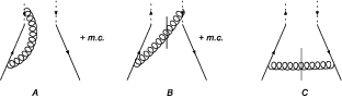
The -correction to the Green function is given by a number of contribution. The corrections to the unsubtracted operator are given by the diagrams shown in fig.4. In the limit and the contribution of individual diagrams reads
| (68) | |||||
| (69) | |||||
| (70) | |||||
where the limit has been taken in the sense of distribution, the factor comes from the scheme, and . The function is
| (71) | |||||
where for the second equality we have assumed that . The function is a shorthand notation for the regular at part of
The quark-field renormalization gives the contribution
| (72) |

The contribution of the soft factor is represented by diagrams in fig.5. Their expression reads
| (73) | |||||
| (74) | |||||
The obtained results in the limit can be compared with the results presented in [17]. They are in agreement up to a finite constant, which is result of different infrared regularization. Also we note the difference by factor two (in comparison with corresponded expression in [17]) for the argument of logarithms of in (74). This is a result of different normalization of light-cone vectors (we use normalization , whereas in [17] is used).
The expression for the second order of the Green function reads
| (75) |
The parameters should be taken according to prescription (36). In the limit this expression reads
| (76) | |||||
where we have also eliminated the terms proportional to and . One can see that this expression is independent on at .
The term , although it does not contribute to any coefficient function at , implies the necessity to introduce the operator (without any fields) into the OPE. The coefficient function of this operator is non-zero with leading term .
The Green function with gluon field at is described by a single diagram shown in fig.6. Due to the absence of tree-order diagram there is no contribution from the soft factor and field renormalization constants. Since we are interested only in the projection of leading twist operators, we average the gluon states over polarizations. In this way the diagrams with Wilson-line – external-gluon interaction vanish. Evaluating the diagram we obtain
| (77) |
where the factor is the result of the gluon-polarization averaging. In the limit this expression reads
| (78) | |||
This result in the limit coincides with the result of calculation performed in [8].

References
- [1] J. Collins, “Foundations of perturbative QCD,” (Cambridge University Press, Cambridge, 2011)
- [2] J. C. Collins, D. E. Soper and G. F. Sterman, Adv. Ser. Direct. High Energy Phys. 5 (1988) 1 [hep-ph/0409313].
- [3] D. Boer, M. Diehl, R. Milner, R. Venugopalan, W. Vogelsang, D. Kaplan, H. Montgomery and S. Vigdor et al., arXiv:1108.1713 [nucl-th].
- [4] C. A. Aidala, B. Field, L. P. Gamberg and T. C. Rogers, arXiv:1401.2654 [hep-ph].
- [5] M. G. Echevarria, A. Idilbi, Z. -B. Kang and I. Vitev, arXiv:1401.5078 [hep-ph].
- [6] J. C. Collins and D. E. Soper, Nucl. Phys. B 193 (1981) 381 [Erratum-ibid. B 213 (1983) 545] [Nucl. Phys. B 213 (1983) 545].
- [7] J. C. Collins and D. E. Soper, Nucl. Phys. B 197 (1982) 446.
- [8] S. M. Aybat and T. C. Rogers, Phys. Rev. D 83 (2011) 114042 [arXiv:1101.5057 [hep-ph]].
- [9] S. M. Aybat, J. C. Collins, J. -W. Qiu and T. C. Rogers, Phys. Rev. D 85 (2012) 034043 [arXiv:1110.6428 [hep-ph]].
- [10] A. Bacchetta and A. Prokudin, Nucl. Phys. B 875 (2013) 536 [arXiv:1303.2129 [hep-ph]].
- [11] H. Bateman, A. Erdelyi, “ Higher Transcendental Functions”, vol.2, (Mc.Graw-Hill Book company, 1953)
- [12] S. V. Mikhailov and A. V. Radyushkin, Nucl. Phys. B 273 (1986) 297.
- [13] X. -d. Ji, J. -p. Ma and F. Yuan, Phys. Rev. D 71 (2005) 034005 [hep-ph/0404183].
- [14] Collins, J.C.: New definition of TMD parton densities. Int. J. Mod. Phys. Conf. Ser. 4, 85 (2011)
- [15] Cherednikov, I.O., Stefanis, N.G.: Renormalization, Wilson lines, and transverse-momentum dependent parton distribution functions. Phys. Rev. D 77, 094001 (2008)
- [16] M. G. Echevarri’a, A. Idilbi and I. Scimemi, Phys. Lett. B 726 (2013) 795 [arXiv:1211.1947 [hep-ph]].
- [17] M. G. Echevarria, A. Idilbi and I. Scimemi, JHEP 1207 (2012) 002 [arXiv:1111.4996 [hep-ph]].
- [18] J. C. Collins and T. C. Rogers, Phys. Rev. D 87 (2013) 3, 034018 [arXiv:1210.2100 [hep-ph]].
- [19] J. -y. Chiu, A. Fuhrer, A. H. Hoang, R. Kelley and A. V. Manohar, Phys. Rev. D 79 (2009) 053007 [arXiv:0901.1332 [hep-ph]].
- [20] A. V. Belitsky, X. Ji and F. Yuan, Nucl. Phys. B 656 (2003) 165 [hep-ph/0208038].