Electric polarizability of neutral hadrons from dynamical lattice QCD ensembles
Abstract
Abstract
We present a valence calculation of the electric polarizability of the neutron, neutral pion, and neutral kaon on two dynamically generated nHYP-clover ensembles. The pion masses for these ensembles are 227(2) MeV and 306(1) MeV, which are the lowest ones used in polarizability studies. This is part of a program geared towards determining these parameters at the physical point. We carry out a high statistics calculation that allows us to: (1) perform an extrapolation of the kaon polarizability to the physical point; we find fm3, (2) quantitatively compare our neutron polarizability results with predictions from PT, and (3) analyze the dependence on both the valence and sea quark masses. The kaon polarizability varies slowly with the light quark mass and the extrapolation can be done with high confidence.
pacs
12.38.GcI Introduction
Determining the polarizability of hadrons has been a challenge both theoretically and experimentally for several decades. To calculate them from first principles, one needs a nonperturbative approach to QCD. In this work we use lattice QCD. The lattice calculation needs to overcome many challenges in order to get to experimentally relevant results, such as the use of smaller quark masses, determining an appropriate field strength for the electric field, volume effects, sea-quark charging effects, etc. In this paper, we will study several of these issues for neutral hadrons (neutron, neutral pion and kaon). Charged hadrons involve additional complications which we defer to future studies.
The neutron polarizability is known experimentally, [1], and therefore a theoretical calculation from first principles provides a good test of QCD. The first experimental determination of the kaon polarizability will be performed as part of the COMPASS [2, 3] experiment along with more precise determination of the pion polarizability.
At the lowest order the effects of an electromagnetic field on hadrons can be parameterized by the effective Hamiltonian:
| (1) |
where and are the static electric and magnetic dipole moments, respectively, and and are the static electric and magnetic polarizabilities. Due to time reversal symmetry of the strong interaction, the static dipole moment, , vanishes. Furthermore, by restricting ourselves to the case of a constant electric field, the leading contribution to the electromagnetic interaction comes from the electric polarizability term at .
There have been several studies on computing the electric polarizabilities in lattice QCD [4, 5, 6, 7, 8]. These calculations, however, were done at relatively large pion masses leaving the chiral region largely unexplored. Here we present a study using two flavors of dynamical nHYP-clover fermions with two different dynamical pion masses (227 and 306 MeV) and several partially quenched valence masses. These pion masses are the lowest pion masses to date for polarizability studies.
Our calculation employs the background field method and uses Dirichlet boundary conditions (DBC) for the valence quarks. This choice of boundary condition has the benefit of allowing us to freely chose an arbitrarily small value for the electric field which is needed in order to extract the polarizability. We note that this work, though done on dynamical configurations, uses electrically neutral sea quarks throughout. Methods for introducing the effect of the electric field on the sea quarks are under investigation [4, 9].
The paper is organized as follows. In Section II we describe our methods used in extracting the polarizability. This includes a discussion of the background field method, how the value of the electric field is chosen, and our fitting procedure. In Section III we present our results for the neutron, pion, and kaon. Section IV is a discussion on the chiral behavior of our results. Lastly we will conclude and outline some future studies in Section V.
II Methodology
II.1 Background Field Method
Electromagnetic properties of hadrons can be determined with the background field method [10]. This procedure introduces the electromagnetic vector potential, , to the Euclidean QCD Lagrangian via minimal coupling; the covariant derivative becomes
| (2) |
where are the gluon field degrees of freedom. The lattice implementation is achieved by a multiplicative U(1) phase factor to the gauge links i.e.,
| (3) |
To achieve a constant electric field, say in the -direction, we may choose which provides us with a real multiplicative factor. The extra factor, , comes from the fact that we are using a Euclidean metric on the lattice. A more convenient choice, and the one implemented in this study, is the use of an imaginary value for the electric field which leads to a U(1) multiplicative factor that keeps the links unitary. When using an imaginary value of the field, the energy shift due to the polarizability acquires an additional negative sign leading to a positive energy shift for a positive value of the polarizability [8]:
| (4) |
To compute this energy shift (and hence the polarizability) we calculate the zero-field (), plus-field (), and minus-field () two-point correlation functions for the interpolating operators of interest. The combination of the plus and minus field correlators allows us to remove any effects, which are statistical artifacts, when the sea quarks are neutral. For neutral particles in a constant electric field the correlation functions still retain their single exponential decay in the limit . In particular we have
| (5) |
where has the perturbative expansion in the electric field given by
| (6) |
By studying the variations of the correlation functions with and without an electric field one can isolate the energy shift to obtain .
For spin-1/2 particles the energy has an additional contribution to its energy shift if the hadron has a magnetic moment, as with the neutron. The interaction of the magnetic moment with the external field contributes to the energy shift at the same order, , as the Compton polarizability [11]. To see this consider a point-like neutral spin-1/2 particle with a non-zero magnetic moment. This system satisfies the Pauli-Dirac equation (in Minkowski space) when subject to an electromagnetic field [12], in particular
| (7) |
where is the electromagnetic field strength tensor. In the non-relativistic limit one can approximate the solution as
| (8) |
In the case of a constant electric field the equation of motion for the upper component satisfies the differential equation
| (9) |
The first term is the usual kinetic term associated with a particle of momentum . The second term is very interesting; in general there is an contribution to the energy shift due to the magnetic moment and momentum of the hadron. It would appear that this term would affect our energy shift since our system has a non-zero momentum due to the DBC (see discussion below). However, this term is zero for our calculations since the direction of the electric field is in the same direction as its induced momentum. The last term is the non-zero contribution due to the magnetic moment of the particle. We see that not only is there a contribution to the energy shift from the Compton polarizability, but also a contribution from the neutron’s magnetic moment. Note that the Compton polarizability acts in the opposite direction of the effects due to the magnetic moment. In the case of a real electric field it lowers the energy whereas the magnetic moment effect increases it. For imaginary fields, as we use in this study, the effect is opposite. The energy expansion is then augmented as
| (10) |
This combination of the Compton polarizability term and the magnetic moment term is what is called the static polarizability,
| (11) |
which is what we measure from the energy shift of the hadron. To obtain the Compton polarizability () we need to account for the magnetic moment. We will address how this is done for the nucleon when presenting our results.

To extract the energy shift we need to choose an appropriate value of . If the field is too large then higher order effects become non-negligble, and if the field is too small we will encounter numerical instabilities in the fitting procedure since the shift to be extracted becomes comparable to the numerical errors introduced by roundoff effects. To ascertain an appropriate field strength we take a single gauge configuration and compute
| (12) |
for the interpolating operator, , to calibrate the field as a function of where is the lattice spacing and is the magnitude of the electric charge for the down quark. The correlator, , is symmetrized with respect to to ensure that there are no linear effects. This symmetrization is achieved by algebraically averaging the plus and minus field correlators. This function is proportional to the effective energy shift and should have a flat behavior in the region where quadratic scaling dominates. Deviations from a constant behavior indicates effects coming from higher order terms in . Fig. 1 shows our findings. We see the effects beyond more dominant for larger times and larger fields. The value is in a well-behaved scaling region for the time slices that we use in our fits and therefore we use this field strength for all our calculations. We checked the behavior for several different configurations on all ensembles used in this work and found similar trends as in Fig. 1.
Several studies used periodic boundary conditions (PBC) in their calculations [5, 6]. In this case, in order to produce a constant electric field, the value of the electric field must be quantized in units of where and are the physical extent of the lattice in the temporal and spatial directions respectively. For the lattice sizes used in this study, the smallest values of which satisfy this quantization condition are and for the and ensembles respectively. These values of are on the periphery where quadratic scaling begins to break down.
To free ourselves of this constraint, we use Dirichlet boundary conditions (DBC) in the direction. This allows us to deploy arbitrarily small values of the field. The use of DBC in the direction of the field introduces boundary effects, one of which is an induced momentum that vanishes in the limit . For an elementary particle in a box of length the induced momentum is and the lowest energy state is . One can observe this effect by looking, for example, at the lowest energy in the pion channel with DBC and PBC. This is shown in Fig. 2. Note the constant shift from the DBC to PBC that corresponds to . Throughout this work we plot the results as a function of the pion mass, as a proxy for the quark mass. This is the pion mass measured using PBC.
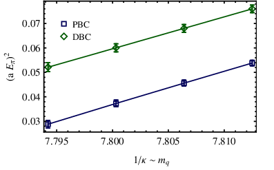
When the hadron is moving, the energy shift () induced by the electric field is not equal to the change in the hadron mass since . We compute the mass shift, , as
| (13) |
where is the zero-momentum mass of the particle which we calculate using PBC.
Using the methods just described we aim to calculate the polarizability of the pion, kaon and neutron. Before proceeding, we should mention that we are only computing the connected contribution to the pion correlation function. The standard interpolating field for the neutral pion is . When the theory is isospin symmetric the disconnected contributions to the two-point correlation function cancel. In the case of an applied external electric field we no longer have isospin symmetry and we should include the disconnected contributions to the correlator. This requires significantly more computational efforts and is thus neglected in this study. We will comment more on this issue in the discussion section.
II.2 Fitting Method
The zero, plus, and minus-field correlation functions are highly correlated because they are constructed from the same gauge configurations. Extracting the energy shift, , then requires a simultaneous-correlated fit among the three correlators. We emphasize that this desired energy shift is very small, several orders of magnitude smaller than the statistical uncertainties of the energy itself. It is because of the correlation that we can extract this tiny shift. Thus, our only hope of extracting such a tiny shift lies in the ability to properly account for the correlations among the three values of the electric field. To do this we construct the following difference vector as
| (14) | |||||
where is the fit window, and . We minimize the function,
in the usual fashion, where is the correlation matrix which has the block structure
where represent , and respectively. Note that the symmetrization is done implicitly in this procedure, since is the same for , and . This method is used to extract all parameters presented in this work.
III Results
III.1 Ensemble Details
The electric polarizabilities of the neutron, pion, and kaon are calculated on two dynamically generated 2-flavor nHYP-clover ensembles [13] with two different sea quark masses to study the chiral behavior. Details of the ensembles are listed in Table 1. The lattice spacing for both ensembles was computed using the Sommer scale [14]. Our calculation of the Sommer parameter, follows the methodology described in [15]. We find to be 4.017(50) and 4.114(39) for ensembles EN1 and EN2, respectively. Using the value of fm yields the lattice spacings listed in Table 1.
| Ensemble | Lattice | (fm) | (MeV) | |||
|---|---|---|---|---|---|---|
| EN1 | 0.1245(16) | 0.12820 | 300 | 25 | ||
| EN2 | 0.1215(11) | 0.12838 | 450 | 18 |

In addition to computing propagators for the sea quark mass we calculated propagators for a string of partially quenched quark masses to gauge the influence of the sea quark mass on the polarizability. The partially quenched values were estimated by looking at the dependence of on for each ensemble. We then performed interpolation in the region where to obtain values of which gave reasonable values of around the dynamical pion masses. The partially quenched and values for each ensemble are tabulated in Table 2.


| Ensemble | Quantity | |||||
|---|---|---|---|---|---|---|
| EN1 | [MeV] | 269(1) | 306(1) | 339(1) | 368(1) | — |
| 0.1283 | 0.1282 | 0.1281 | 0.1280 | — | ||
| EN2 | [MeV] | 227(2) | 283(1) | 322(1) | 353(1) | 382(1) |
| 0.12838 | 0.12825 | 0.12814 | 0.12804 | 0.12794 |
An optimally implemented multi-GPU Dslash operator [16], along with an efficient BiCGstab multi-mass inverter [17] was used to compute all correlation functions in this work.
For the kaon polarizability we needed to include a valence mass for the strange quark. To this end we determined an appropriate value of by measuring the mass of the baryon and the meson. We computed the mass of the baryon and meson for a string of values. We then performed interpolation among these masses to match the physical value of each hadron and took the average of the two values. We find for the EN1 ensemble and for the EN2 ensemble.
III.2 Extracted Parameters
To reduce our statistical uncertainties we computed quark propagators at multiple point sources for each configuration. The number of sources used in each ensemble is listed in Table 1. The sources were chosen by selecting points which are related by translational symmetry. This is achieved by varying the source position only along the and axes—these directions remain translationally invariant since we use PBC in these directions.
To observe the benefits of multiple sources we study the behavior of the statistical error of the energy shift as a function of the number of sources, . Fig. 3 shows such scaling plots.
In determining the number of sources to compute one should look at the scaling of the statistical error for the different hadrons of interest. For example, if one were to look only at the pion then it would seem that little or nothing is gained from using more than sources. However, for the neutron we observe a decrease in the uncertainties relative to the pion for up to 25 sources. A similar plateau region for the neutron is expected to occur as more sources are added since the source locations become more dense and hence more correlated.
To quote a value of we need to determine an appropriate time window to fit the correlators. Our fit region is chosen by varying the minimum time distance and computing , and for each ensemble and particle of interest. We choose our fit window based on the stability of the parameters as a function of , and on a reasonable value of . Fig. 4 shows an example of this for the extracted energy shift of the neutron on the EN2 ensemble at the unitary point, i.e., the point where the sea quark mass is equal to the valence mass. The value of was held fixed at . A similar analysis was performed at neighboring values of and we find the same behavior in each case. For both ensembles and each hadron we determined the fit range using the procedure just described for the unitary point. We then kept that fit window fixed for all other partially-quenched values. Table 3 lists the time ranges used to extract the energy shifts for each hadron on the two ensembles.


| Ensemble | Pion | Kaon | Neutron |
|---|---|---|---|
| EN1 | [14,30] | [14,30] | [8,21] |
| EN2 | [15,36] | [15,37] | [9,23] |

Our computed values for the neutral pion and kaon polarizabilites are presented in Table 4. Tables 5 and 6 list the extracted energy shift and masses respectively. The static polarizabilities were computed from the mass shift via the equation:
| (15) |
Eq.(15) is readily obtained by recalling that the mass shift is connected to the polarizability via and . The left panel of Fig. 5 shows our results for the kaon and the left panel of Fig. 7 shows our results for the pion, both as a function of . For the pion polarizability we also overlay quenched results from the study done in [19], we will comment on this in the discussion section.
To obtain the neutron Compton polarizability we use the energy expansion given in Eq.(10) which depends on its anomalous magnetic moment . In our analysis we did not measure directly. Instead we perform an extrapolation to the values of as a function of determined from an independent study [18]. We use a quadratic fit, as was done in [18], to find as a function of . In units of the nuclear magneton, , we find
| (16) | |||||
| where | |||||
| and |
Fig. 6 shows the fit to the data points from [18]. This fitting form is motivated by PT [20]. By comparing our fit with lattice results at lower pion mass [21], we estimate that our systematic errors are less than 5%. Given that the magnetic moment contributes at most 20% to the mass shift the overall systematic associated with this procedure is on the order of 1%. This is significantly smaller than our stochastic errors on the polarizability.
Using the above functional form for we can now compute the Compton neutron polarizability by
| (17) |
where is given by Eq.(15) and is the mass of the neutron measured from the lattice in physical units.
IV Discussion
In this section we will discuss some features in our results for the kaon, pion, and neutron individually.


IV.1 Neutral Kaon
Beginning first with the kaon, we see from the left panel of Fig. 5 that the polarizability depends on the sea quark mass even when the valence quark mass is kept fixed. We note that the change in the polarizability is small in absolute terms. The difference between the two sea quark masses is only 0.1 in units of (the “natural” units for hadron polarizability) when the light quark mass is almost halved. The kaon polarizability also changes very little when the valence quark mass is varied.
This slow change as a function of allows us to do a trustworthy extrapolation to the physical point. To perform this extrapolation, we use the two values at the unitary points and the result determined in [6] for the kaon polarizability at . The fit assumes a linear dependence on . The results of our extrapolation are shown in the right panel Fig. 5. We find . The kaon polarizability has not yet been measured experimentally. PT predicts the polarizability to be zero at [22]. Our result is consistent with PT since the kaon polarizability is relatively small in units of .
There are systematic errors associated with our study. One of them is the tuning of . Recall from section III.1 that we tuned the value of so that the masses of the baryon and the meson matched their physical values. This procedure, however, produces different kaon masses for the EN1 and EN2 ensembles for comparable light quark masses. This is due to a difference in the strange quark mass on the two ensembles. We do not expect this to affect the polarizability significantly. This is supported by the plot in the left panel of Fig. 5 where we can see that the polarizability is insensitive to the value of the valence light quark mass. We expect the same level of insensitivity with respect to the valence strange quark mass.
IV.2 Neutral Pion
Next we turn to the pion polarizability. In the left panel of Fig. 7 we overlay the results of our study along with quenched results found in [19]. This comparison among all three data sets tells us that the pion polarizability, at the level of our error bars, is relatively insensitive to the sea quark mass. The quenched ensemble is interpreted as a system where the sea quarks are infinitely heavy.
We note that the negative trend that has been seen in previous studies [6, 19] is still present. We would like to re-iterate what was mentioned in [6]: The expectation of PT at order and is that the polarizability is about [23]. This value is consistent with what we have computed. However, the PT results come only from disconnected contributions to the correlation function, which was neglected in our calculation. Without the disconnected contribution it is expected that the polarizability is substantially smaller and positive (see [6]). It was suggested that perhaps this was due to finite-volume effects. However, the study done in [19] and preliminary studies in [24] show that this is not the case. This puzzling result could also come from the fact that we have left out the effects of coupling the charge of the sea quarks to the electric field. Different methods to include the effects due to charging of the sea quarks are being explored [9] .
IV.3 The Neutron


In the right panel of Fig. 7 we plot our results for neutron polarizability. We see that the dependence on the sea quark mass is more pronounced than in the meson case. Our results are compatible with the quenched ones, at least qualitatively. The large error bars for the quenched results make a more quantitative evaluation impossible. Turning to our results, we see that the polarizability rises when the quark mass is decreased, as anticipated. The change in the valence mass produces only a slight increase, whereas the sea quark mass change plays a more important role.
We compare now our findings for the neutron polarizability to two different PT predictions: PT [25, 26] and PT [27]. We use this comparison to gauge the systematic errors of our calculation, in particular finite volume effects and neglecting the electric charge of the sea quarks. These two PT curves use different approximations in their calculations to derive the chiral form. In the case of PT the calculation is expanded to N2LO using a non-relativistic form for the propagators. There are two extra free parameters which are determined by fitting to Compton scattering data. The second result, PT, includes terms up to NLO and uses relativistic propagators. They compute as a function of with no free parameters. The error bars in PT come from a careful analysis [28] whereas the error bar for the second curve is fixed to a value estimated at the physical point.
The left panel of Fig. 8 shows the two PT curves along with our findings. Our results for both ensembles seem to be in agreement more with the PT curve for our 306 MeV pion. However, our lattice calculation is in disagreement with both curves at the 227 MeV pion. We believe that this is due to finite-volume effects and the fact that the sea quarks are electrically neutral.
To gauge the effect of charging the sea quarks we use PT [29]: for the pion mass between and when the sea quarks are charged the polarizability increases by –. This would explain part of the discrepancy seen between our data at and the PT curves shown in Fig. 8. However, significant differences still remain and we believe that this is due to finite volume effects.
Finite volume corrections can also be estimated using PT. For periodic boundary conditions these effects were calculated for electric polarizabilities [29] and magnetic polarizabilities [30]. For MeV and it was found that the correction to is about 7% [29]. However, we used DBC in this work and we expect that these corrections will be more important than for PBC. This is supported by the discrepancy we have between our results and PT predictions, as discussed above, and sigma model studies for chiral condensate in the presence of hard walls [31]. Further studies are required to determine the magnitude of these corrections.
V Conclusion
We performed a valence calculation of the electric polarizabilites of the neutral pion, neutral kaon, and neutron using a two-flavor nHYP clover action at two dynamical pion masses: 306 MeV and 227 MeV. These are to date the lowest pion masses used for polarizability studies. A chiral extrapolation for the kaon was performed using three dynamical points including the 400 MeV point from [6]. We find the neutral kaon polarizability to be . The chiral behavior of the kaon is fairly mild, suggesting that the systematic errors for our extrapolated value are similarly mild. For the pion, the negative trend remains to be understood. We speculate that this may be due to the fact that we have neglected the charge of the sea quarks and we are working on including these effects [9]. Our neutron polarizability results are promising. The stochastic errors are significantly smaller than other lattice studies and we also have the lightest dynamical quark masses. We note that our errors are significantly smaller than the ones from PT studies. The hope is that when the finite-volume systematics are removed and the sea quarks are charged we will be able to constrain the parameters in the PT models. This in turn could be used to tighten the error bars on the PT predictions at the physical point and make the comparison with the experimentally measured values more informative.
Acknowledgements.
We would like to thank Craig Pelissier for generating the ensembles used in this study. Also many thanks to Harald Grießhammer and Vladimir Pascalutsa for providing us with the PT curves for the neutron polarizability. The computations were carried out on a variety of GPU-based platforms, including the IMPACT clusters and Colonial One at GWU, the clusters at JLab and FermiLab, and the clusters at University of Kentucky. This work is supported in part by the NSF CAREER grant PHY-1151648, the U.S. Department of Energy grant DE-FG02-95ER40907, and the ARCS foundation.References
- [1] J. Beringer et. al. (Particle Data Group Collaboration), Phys.Rev. D86 (2012) 010001.
- [2] P. Abbon et. al. (COMPASS Collaboration), Nucl.Instrum.Meth. A577 (2007) 455–518, [hep-ex/0703049].
- [3] T. Nagel, S. Paul, and J. M. Friedrich, Measurement of the Charged Pion Polarizability at COMPASS. PhD thesis, Munich Tech. U., Sep, 2012. Presented 27 Sep 2012.
- [4] M. Engelhardt (LHPC Collaboration), Phys.Rev. D76 (2007) 114502, [arXiv:0706.3919].
- [5] W. Detmold, B. Tiburzi, and A. Walker-Loud, Phys.Rev. D81 (2010) 054502, [arXiv:1001.1131].
- [6] W. Detmold, B. C. Tiburzi, and A. Walker-Loud, Phys.Rev. D79 (2009) 094505, [arXiv:0904.1586].
- [7] H. Fiebig, W. Wilcox, and R. Woloshyn, Nucl.Phys. B324 (1989) 47.
- [8] A. Alexandru and F. X. Lee, PoS LATTICE2008 (2008) 145, [arXiv:0810.2833].
- [9] W. Freeman, A. Alexandru, F. Lee, and M. Lujan, PoS LATTICE2012 (2012) 015, [arXiv:1211.5570].
- [10] G. Martinelli, G. Parisi, R. Petronzio, and F. Rapuano, Phys.Lett. B116 (1982) 434.
- [11] A. L’vov, Int.J.Mod.Phys. A8 (1993) 5267–5303.
- [12] G. Burling-Claridge and P. H. Butler, J.Phys. G15 (1989) 571–582.
- [13] A. Hasenfratz, R. Hoffmann, and S. Schaefer, JHEP 0705 (2007) 029, [hep-lat/0702028].
- [14] R. Sommer, Nucl.Phys. B411 (1994) 839–854, [hep-lat/9310022].
- [15] C. Pelissier and A. Alexandru, Phys.Rev. D87 (2013) 014503, [arXiv:1211.0092].
- [16] A. Alexandru, M. Lujan, C. Pelissier, B. Gamari, and F. X. Lee, in Application Accelerators in High-Performance Computing (SAAHPC), 2011 Symposium on, pp. 123 –130, 2011, [arXiv:1106.4964].
- [17] A. Alexandru, C. Pelissier, B. Gamari, and F. Lee, J.Comput.Phys. 231 (2012) 1866–1878, [arXiv:1103.5103].
- [18] F. Lee, R. Kelly, L. Zhou, and W. Wilcox, Phys.Lett. B627 (2005) 71–76, [hep-lat/0509067].
- [19] A. Alexandru and F. Lee, PoS LATTICE2010 (2010) 131, [arXiv:1011.6309].
- [20] J. Hall, D. Leinweber, and R. Young, Phys.Rev. D85 (2012) 094502, [arXiv:1201.6114].
- [21] T. Primer, W. Kamleh, D. Leinweber, and M. Burkardt, Phys.Rev. D89 (2014) 034508, [arXiv:1307.1509].
- [22] F. Guerrero and J. Prades, Phys.Lett. B405 (1997) 341–346, [hep-ph/9702303].
- [23] J. Portoles and M. Pennington, [hep-ph/9407295].
- [24] M. Lujan, A. Alexandru, W. Freeman, and F. Lee, [arXiv:1310.4837].
- [25] H. Griesshammer, J. McGovern, D. Phillips, and G. Feldman, Prog.Part.Nucl.Phys. 67 (2012) 841–897, [arXiv:1203.6834].
- [26] J. McGovern, D. Phillips, and H. Griesshammer, Eur.Phys.J. A49 (2013) 12, [arXiv:1210.4104].
- [27] V. Lensky and V. Pascalutsa, Eur.Phys.J. C65 (2010) 195–209, [arXiv:0907.0451].
- [28] H. Griesshammer, J. McGovern, and D. Phillips, in preparation.
- [29] W. Detmold, B. C. Tiburzi, and A. Walker-Loud, Phys. Rev. D 73 (Jun, 2006) 114505.
- [30] J. Hall, D. Leinweber, and R. Young, [arXiv:1312.5781].
- [31] B. Tiburzi, Phys. Rev. D 88, 034027 (2013) 034027, [arXiv:1302.6645].
| [] | ||||||||||
|---|---|---|---|---|---|---|---|---|---|---|
| Hadron | EN1 | c | EN2 | |||||||
| Hadron | EN1 | c | EN2 | |||||||
|---|---|---|---|---|---|---|---|---|---|---|
| Hadron | EN1 | c | EN2 | |||||||
|---|---|---|---|---|---|---|---|---|---|---|