Multiple scattering by randomly placed particles frustrates the passage of light through ‘opaque’ materials such as turbid water, white paint, and egg shells. Thanks to the theoretical work of Dorokhov [8], Barnes and Pendry et al. [28, 2], and others [25, 3], as well as the breakthrough experiments of Vellekoop and Mosk [43, 44] and others [29, 20, 31, 19, 40, 1, 6, 7, 37], we now understand that even though a normally incident wavefront will barely propagate through a thick slab of such media [16], a small number of eigen-wavefronts exist that exhibit a transmission coefficient close to one and hence propagate through the slab without significant loss.

In highly scattering random media composed of non-absorbing scatterers, these ‘perfectly transmitting’ eigen-wavefronts are the right singular vectors of the modal transmission matrix with singular values (or transmission coefficients) close to $1$. Thus, if the modal transmission matrix were measured using the techniques described in [29, 20, 31, 19], one could compute the pertinent singular vector and synthesize a highly transmitting eigen-wavefront via spatial amplitude and phase modulation. The task of amplitude and phase modulating an optical wavefront is not, however, trivial. Calibration and alignment issues prevent the use of two independent spatial light modulators in series that separately modulate the signal amplitude and phase. A viable option is to use the innovative method developed by van Putten et al. in [41] for full spatial phase and amplitude control using a twisted nematic LCD combined with a spatial filter.

In a recent paper [17, 18], we assumed that amplitude and phase modulation was feasible, and developed iterative, physically-realizable algorithms for synthesizing highly transmitting eigen-wavefronts using just a few measurements of the backscatter field. We showed that the algorithms converge rapidly and achieve $95\%$ transmission using about $5-10$ measurements. Our focus on constructing highly transmitting eigen-wavefronts by using the information in the backscatter field was motivated by biomedical applications, where it is often impossible to measure transmitted fields. Our work will be most helpful in settings where it is desirable to increase the amount of light transmitted through an intervening scattering medium such as in photodynamic therapy where a photosynthesizing agent on exposure to light produces a form of oxygen that can kill neighboring (cancerous) cells [9]. Another promising application is in photoacoustic imaging [45] which exploits the photoacoustic effect whereby light is converted into heat by absorbing scatterers and the subsequent thermoelasctic expansion produces wideband ultrasonic emissions which can be detected by ultrasonic transducers to form images. Recent breakthrough works have taken this a step further by exploiting the photoacoustic effect to focus light within the medium [21, 4]. Since the strength of the photoacoustic effect is proportional to the scattered light intensity at the light absorber, one might reasonably expect that algorithms, such as ours, that can increase the amount of transmitted light through a medium can help improve the penetration depth of photoacoustic imaging (or photoacoustic imaging guided focusing) by inducing stronger photoacoustic signals from deeper in the medium.

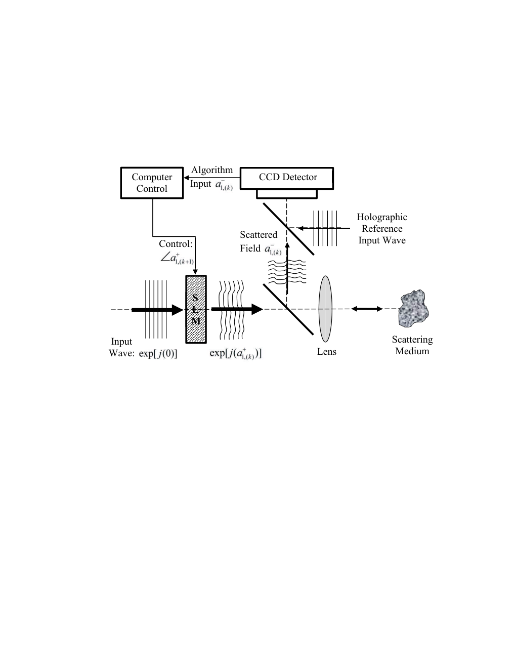
Here, we place ourselves in the setting where we seek to increase transmission via backscatter analysis but are restricted to phase-only modulation. The phase-only modulation constraint was initially motivated by the simplicity of the resulting experimental setup (see Fig. 1) and the commercial availability of finely calibrated phase-only spatial light modulators (SLMs) (e.g. the PLUTO series from Holoeye). As we shall shortly see there is another engineering advantage conferred by these methods. We do not, however, expect to achieve perfect transmission using phase-only modulation as is achievable by amplitude and phase modulation. However, we theoretically show that we can expect to get at least (about) $25\pi\%\approx 78.5\%$ provided that 1) the system modal reflection (or transmission) matrix is known, 2) its right singular vectors obey a maximum entropy principle by being isotropically random, and 3) full amplitude and phase modulation permits at least one perfectly transmitting wavefront. We also develop iterative, physically realizable algorithms for transmission maximization that utilize backscatter analysis to produce a highly transmitting phase-only modulated wavefront in just a few iterations. These rapidly converging algorithms build on the ideas developed in [17, 18] by incorporating the phase-only constraint. An additional advantage conferred by these rapidly converging algorithms is that they might facilitate their use in applications where the duration in which the modal transmission or reflection matrix can be assumed to be constant is relatively small compared to the time it would take to make all measurements needed to estimate the modal transition or reflection matrix or in settings where a near-optimal solution obtained fast is preferable to the optimal solution that takes many more measurements to compute. As in [18], the iterative algorithms we have developed retain the feature that they allow the number of modes being controlled via an SLM in experiments to be increased without increasing the number of measurements that have to be made.

We numerically analyze the limits of phase-only modulated transmission in 2-D with fully spectrally accurate simulators and provide rigorous numerical evidence confirming our theoretical prediction in random media with periodic boundary conditions that is composed of hundreds of thousands of non-absorbing scatterers. Specifically, we show that the best performing iterative algorithm yields $\approx 70\%$ transmission using just $15-20$ measurements in the regime where the non-iterative algorithms yield $\approx 78.5\%$ transmission.

This theoretical prediction brings into sharp focus an engineering advantage to phase-only modulation relative to amplitude and phase modulation that we did not anticipate when we embarked on this line of inquiry. The clever idea in van Putten et al’s work was to use spatial filtering to combine four neighboring pixels into one superpixel and then independently modulate the phase and the amplitude of light at each superpixel. This implies that an SLM with $M$ pixels can control at most $M/4$ spatial modes. For a given aperture, combining neighboring pixels into one super pixel corresponds to passing the entire wavefront into a spatial low pass filter. We argue that in critically or undersampled scenarios phase-only measurements permit the design of more highly transmitting wavefronts than amplitude-phase measurements that use the idea of van Putten et al.

For highly scattering random media, our numerical results in Section 7, suggest that undersampling the spatial modes by $75\%$ will reduces the average amount of transmission by between $65-75\%$. In contrast, our theoretical results in Section 5 show that controlling all $M$ spatial modes using phase-only modulation will reduce the average amount transmission by at most $30\%$. Thus, we can, on average, achieve higher transmission with phase-only modulation using all the pixels in an SLM than by (integer-valued) undersampling of the pixels to implement amplitude and phase modulation! The paper is organized as follows. We describe our setup in Section 2. We discuss the problem of transmission maximization using phase-only modulated wavefronts in Section 3. We describe physically realizable, non-iterative and iterative algorithms for transmission maximization in Section 4 and in Section 6, respectively. We identify fundamental limits of phase-only modulated transmission in Section 5, validate the predictions and the rapid convergence behavior of the iterative algorithms in Section 7, and summarize our findings in Section 8.

We study scattering from a two-dimensional (2D) periodic slab of thickness $L$ and periodicity $D$. The slab’s unit cell occupies the space $0\leq x<D$ and $0\leq y<L$ (Fig. 2) and contains $N_{c}$ infinite and $z$-invariant circular cylinders of radius $r$ that are placed randomly within the cell and assumed either perfect electrically conducting (PEC) or dielectric with refractive index $n_{d}$. Care is taken to ensure the cylinders do not overlap. All fields are $\sf TM_{\mbox{$z$}}$ polarized: electric fields in the $y<0$ $(i=1)$ and $y>L$ $(i=2)$ halfspaces are denoted $\underline{e}_{i}(\underline{\rho})=e_{i}(\underline{\rho})\hat{z}$. These fields (complex) amplitudes $e_{i}(\underline{\rho})$ can be decomposed in terms of $+y$ and $-y$ propagating waves as $e_{i}(\underline{\rho})=e_{i}^{+}(\underline{\rho})+e_{i}^{-}(\underline{\rho})$, where

$$e^{\pm}_{i}(\underline{\rho})=\displaystyle\sum_{n=-N}^{N}h_{n}a^{\pm}_{i,n}e^{-j\underline{k}^{\pm}_{n}\cdot\underline{\rho}}\,.$$

(1)

In the above expression, $\underline{\rho}=x\hat{x}+y\hat{y}\equiv(x,y)$, $\underline{k}^{\pm}_{n}=k_{n,x}\hat{x}\pm k_{n,y}\hat{y}\equiv(k_{n,x},\pm k_{n,y})$, $k_{n,x}=2\pi n/D$, $k_{n,y}=2\pi\sqrt{(1/\lambda)^{2}-(n/D)^{2}}$, $\lambda$ is the wavelength, and $h_{n}=\sqrt{\|\underline{k}^{\pm}_{n}\|_{2}/k_{n,y}}$ is a power-normalizing coefficient. We assume $N=\lfloor D/\lambda\rfloor$, i.e., we only model propagating waves and denote $M=2N+1$. The modal coefficients $a^{\pm}_{i,n}$, $i=1,2$; $n=-N,\ldots,N$ are related by the scattering matrix

$$\left[\begin{array}[]{c}\underline{a}^{-}_{1}\\ \underline{a}^{+}_{2}\\ \end{array}\right]=\underbrace{\left[\begin{array}[]{cc}S_{11}&S_{12}\\ S_{21}&S_{22}\end{array}\right]}_{=:S}\left[\begin{array}[]{c}\underline{a}^{+}_{1}\\ \underline{a}^{-}_{2}\\ \end{array}\right],$$

(2)

where $\underline{a}^{\pm}_{i}=\begin{bmatrix}a^{\pm}_{i,-N}&\ldots&a^{\pm}_{i,-1}&a^{\pm}_{i,0}&a^{\pm}_{i,1}&\ldots&a^{\pm}_{i,N}\end{bmatrix}^{T}$ and ^T denotes transposition. In what follows, we assume that the slab is only excited from the $y<0$ halfspace; hence, $\underline{a}^{-}_{2}=0$. For a given incident field amplitude $e^{+}_{1}(\underline{\rho})$, we define transmission and reflection coefficients as

	$\displaystyle\tau(\underline{a}^{+}_{1}):=\dfrac{\|S_{21}\cdot\underline{a}^{+}_{1}\|_{2}^{2}}{\|\underline{a}^{+}_{1}\|_{2}^{2}},$		(3)
and
	$\displaystyle\gamma(\underline{a}^{+}_{1}):=\dfrac{\|S_{11}\cdot\underline{a}^{+}_{1}\|_{2}^{2}}{\|\underline{a}^{+}_{1}\|_{2}^{2}},$		(4)

respectively. We denote the transmission coefficient of a normally incident wavefront by $\tau_{\sf normal}=\tau(\begin{bmatrix}0&\cdots&0&1&0&\cdots&0\end{bmatrix}^{T})$.

We define the phase-vector of the modal coefficient vector $\underline{a}^{+}_{1}$, as

$$\vbox to8.46227pt{\hbox{\begin{picture}\put(0.0,0.0){\circle*{0.4}}\put(0.0,0.0){\line{1}{0}{17.37354}}\put(0.0,0.0){\line{1}{2}{5.7346}}\put(5.7346,1.5){\raise 1.5pt\vbox{\hbox{$\textstyle\underline{a}^{+}_{1}$}}}\end{picture}}\vss}=\begin{bmatrix}\quad\vbox to7.96227pt{\hbox{\begin{picture}\put(0.0,0.0){\circle*{0.4}}\put(0.0,0.0){\line{1}{0}{27.98027}}\put(0.0,0.0){\line{1}{2}{6.16516}}\put(6.16516,1.5){\raise 2.8611pt\vbox{\hbox{$\textstyle a_{1,-N}^{+}$}}}\end{picture}}\vss}&\cdots&\vbox to7.96227pt{\hbox{\begin{picture}\put(0.0,0.0){\circle*{0.4}}\put(0.0,0.0){\line{1}{0}{22.18721}}\put(0.0,0.0){\line{1}{2}{6.16516}}\put(6.16516,1.5){\raise 2.8611pt\vbox{\hbox{$\textstyle a_{1,0}^{+}$}}}\end{picture}}\vss}&\cdots&\vbox to7.96227pt{\hbox{\begin{picture}\put(0.0,0.0){\circle*{0.4}}\put(0.0,0.0){\line{1}{0}{27.98027}}\put(0.0,0.0){\line{1}{2}{6.16516}}\put(6.16516,1.5){\raise 2.8611pt\vbox{\hbox{$\textstyle a_{1,-N}^{+}$}}}\end{picture}}\vss}\quad\end{bmatrix}^{T},$$

where for $n=-N,\ldots,N$, $a_{1,n}^{+}=|a_{1,n}^{+}|\exp(j\vbox to7.96227pt{\hbox{\begin{picture}\put(0.0,0.0){\circle*{0.4}}\put(0.0,0.0){\line{1}{0}{23.14441}}\put(0.0,0.0){\line{1}{2}{6.16516}}\put(6.16516,1.5){\raise 2.8611pt\vbox{\hbox{$\textstyle a_{1,n}^{+}$}}}\end{picture}}\vss})$ and $|a_{1,n}^{+}|$ and

$a1,n+$ denote the magnitude and phase of $a_{1,n}^{+}$, respectively. Let ${P}_{1}^{M}$ denote unit-norm vectors of the form

$$\underline{p}(\underline{\theta})=\sqrt{\dfrac{1}{M}}\begin{bmatrix}e^{j\theta_{-N}}&\cdots&e^{j\theta_{0}}&\cdots&e^{j\theta_{N}}\end{bmatrix}^{T},$$

(5)

where $\underline{\theta}=\begin{bmatrix}\theta_{-N}&\cdots&\theta_{0}&\cdots&\theta_{N}\end{bmatrix}^{T}$ is a $M\times 1$ vector of phases where $M:=2N+1$. Then, the problem of designing a phase-only modulated incident wavefront that maximizes the transmitted power can be stated as

$$\underline{a}_{\sf opt}=\argmax_{\underline{a}^{+}_{1}\in P_{1}^{M}}\tau(\underline{a}^{+}_{1})=\argmax_{\underline{a}^{+}_{1}\in P_{1}^{M}}\|S_{21}\cdot\underline{a}^{+}_{1}\|_{2}^{2}.$$

(6)

In the lossless setting, the scattering matrix $S$ in Eq. (2) will be unitary, i.e., $S^{H}\cdot S=I$, where $I$ is the identity matrix. Consequently, we have that

$$S_{11}^{H}\cdot S_{11}+S_{21}^{H}\cdot S_{21}=I,$$

(7)

so that the $\|S_{21}\cdot\underline{a}^{+}_{1}\|_{2}=\sqrt{1-\|S_{11}\cdot\underline{a}^{+}_{1}\|_{2}^{2}}$ and the optimization problem in Eq. (6) can be reformulated as

$$\underline{a}_{\sf opt}=\argmin_{\underline{a}^{+}_{1}\in P_{1}^{M}}\|S_{11}\cdot\underline{a}^{+}_{1}\|_{2}=\argmin_{\underline{a}^{+}_{1}\in P_{1}^{M}}\gamma(\underline{a}^{+}_{1}).$$

(8)

Thus the phase-only modulated wavefront that maximizes transmission will also minimize backscatter. The feasible set in Eq. (8) is non-convex since for $\theta_{1}\neq\theta_{2}$ and $\alpha\in(0,1)$, $\alpha\,\underline{p}(\underline{\theta}_{1})+(1-\alpha)\underline{p}(\underline{\theta}_{2})\notin P_{1}^{M}$. Moreover, it is known [35] that Eq. (8) does not admit a closed-form solution for $\underline{a}_{\sf opt}$ (and hence $\underline{\theta}_{\sf opt}$ ). Thus we turn our attention to computational methods for solving Eq. (8).

We first consider algorithms for increasing transmission by backscatter minimization using phase-only modulated wavefronts that utilize measurements of the reflection matrix $S_{11}$. We assume that this matrix can be measured using the experimental techniques described in [29, 20, 31, 19] by, in essence, transmitting $K>M$ incident wavefronts $\{\underline{a}_{1,i}^{+}\}_{i=1}^{K}$, measuring the (modal decomposition of the) backscattered wavefronts $\{\underline{a}_{1,i}^{-}\}_{i=1}^{K}$ and estimating $S_{11}$ by solving the system of equations $\{\underline{a}_{1,i}^{-}=S_{11}\cdot\underline{a}_{1,i}^{+}\}_{i=1}^{K}$. We note that, even if the $S_{11}$ matrix has been measured perfectly, the optimization problem in Eq. (8) is computationally intractable and known to be NP-hard [46, Proposition 3.3],[23]. We can make the problem computationally tractable by relaxing the phase-only constraint in Eq. (8) and allowing the elements of $\underline{a}^{+}_{1}$ to take on arbitrary amplitudes and phases while imposing the power constraint $\parallel\underline{a}^{+}_{1}\parallel^{2}=1$. This yields the optimization problem

$$\underline{a}_{\sf svd}=\argmin_{\parallel\underline{a}^{+}_{1}\parallel_{2}=1}\|S_{11}\cdot\underline{a}^{+}_{1}\|_{2}^{2},$$

(9)

where we have relaxed the difficult constraint $\underline{a}^{+}_{1}\in P_{1}^{M}$ into the spherical constraint $||\underline{a}^{+}_{1}||_{2}=1$. The problem in Eq. (9) can be solved exactly as described next.

Let $S_{21}=\sum_{i=1}^{M}{\sigma}_{i}\underline{{u}}_{i}\cdot\underline{{v}}_{i}^{H}$ and $S_{11}=\sum_{i=1}^{M}\widetilde{\sigma}_{i}\underline{\widetilde{u}}_{i}\cdot\underline{\widetilde{v}}_{i}^{H}$ denote the singular value decompositions (SVD) of $S_{21}$ and $S_{11}$, respectively. Here $\sigma_{i}$ (resp. $\widetilde{\sigma}_{i}$) is the singular value associated with the left and right singular vectors $\underline{u}_{i}$ and $\underline{v}_{i}$ (resp. $\underline{\widetilde{u}}_{i}$ and $\underline{\widetilde{v}}_{i}$), respectively. By convention, the singular values are arranged so that $\sigma_{1}\geq\ldots\geq\sigma_{M}$ and ${\widetilde{\sigma}}_{1}\geq\ldots\geq{\widetilde{\sigma}}_{M}$ and ^H denotes the complex conjugate transpose. The solution to Eq. (9) can be expressed in terms of the right singular vectors of $S_{11}$ and $S_{21}$ as

$$\underline{a}_{\sf svd}=\widetilde{\underline{v}}_{M}=\underline{v}_{1}.$$

(10)

In Eq. (10), we have employed the well-known variational characterization [14, Theorem 7.3.10] of the smallest right singular vector for the first equality and the identity $\underline{v}_{i}=\widetilde{\underline{v}}_{M-i+1}$ derived from Eq. (7) for the second equality. This is an exact solution to the relaxed backscatter minimization problem in Eq. (9).

To get an approximation of the solution to the original unrelaxed problem in Eq. (8) we construct a wavefront as

$$\underline{a}_{\sf opt,svd}=\underline{p}\left({\vbox to5.67776pt{\hbox{\begin{picture}\put(0.0,0.0){\circle*{0.4}}\put(0.0,0.0){\line{1}{0}{21.03679}}\put(0.0,0.0){\line{1}{2}{4.34236}}\put(4.34236,1.5){\raise 1.5pt\vbox{\hbox{$\textstyle\,\underline{a}_{\sf svd}$}}}\end{picture}}\vss}}\right).$$

(11)

The spherical relaxation that yields the optimization problem in Eq. (9) includes all the phase-only wavefronts in the original problem, but also includes many other wavefronts as well. We now consider a ‘tighter’ semidefinite programming (SDP) relaxation that includes all the phase-only wavefronts in the original problem but fewer other wavefronts than the spherical relaxation does.

We note that SDP relaxations to computationally intractable problems such as Eq. (8) have gained in popularity in recent decades because there are many problems in the literature for which the SDP relaxation is known to provide a constant relative accuracy estimate for the exact solution to the unrelaxed problem [11, 26, 27]. We shall provide a similar constant relative accuracy estimate for our problem shortly in Eq. (17).

We begin by examining the objective function on the right hand side of Eq. (9). Note that

$$||S_{11}\cdot\underline{a}^{+}_{1}||_{2}^{2}=\left((\underline{a}^{+}_{1})^{H}\cdot S_{11}^{H}\cdot S_{11}\cdot\underline{a}^{+}_{1}\right)=\textrm{Tr}\left(S_{11}^{H}\cdot S_{11}\cdot\underline{a}^{+}_{1}\cdot(\underline{a}^{+}_{1})^{H}\right),$$

(12)

where $\textrm{Tr}(\cdot)$ denotes the trace of its matrix argument. Let us define a new matrix-valued variable $A=\underline{a}^{+}_{1}\cdot(\underline{a}^{+}_{1})^{H}$. We note that $A$ is a Hermitian, positive semi-definite matrix with rank $1$ and $A_{ii}=1/M$ whenever $\underline{a}^{+}_{1}\in P_{1}^{M}$, where $A_{ii}$ denotes the $i$th diagonal element of the matrix $A$. Consequently, from Eq. (12), we can derive the modified optimization problem

	$\displaystyle{A}_{\sf opt}=$	$\displaystyle\argmin_{A\in\mathbb{C}^{M\times M}}\textrm{Tr}\left(S_{11}^{H}\cdot S_{11}\cdot A\right)$		(13)
		$\displaystyle\text{subject to }A=A^{H},A\succeq 0,\textrm{rank}(A)=1\textrm{ and }A_{ii}=1/M\textrm{ for }i=1,\ldots M,$

where the conditions $A=A^{H}$ and $A\succeq 0$ imply that $A$ is a Hermitian, positive semi-definite matrix. If we can solve Eq. (13) exactly, then by construction, since $A_{\sf opt}$ is rank $1$, we must have that $A_{\sf opt}=\underline{a}_{\sf opt,eig}\cdot\underline{a}_{\sf opt,eig}^{H}$ with $\underline{a}_{\sf opt,eig}\in P_{1}^{M}$ so we would have solved Eq. (8) exactly. Note that the set of rank one matrices is non-convex since the sum of two rank one matrices is not necessarily rank one. Thus the rank constraint in Eq. (13) makes the problem difficult to solve [23] even though the objective function and other constraints are convex in $A$.

Eliminating the difficult rank constraint yields the semi-definite programming (SDP) problem [42]

	$\displaystyle A_{\sf sdp}=$	$\displaystyle\argmin_{A\in\mathbb{C}^{M\times M}}\textrm{Tr}\left(S_{11}^{H}\cdot S_{11}\cdot A\right)$		(14)
		$\displaystyle\text{subject to }A=A^{H},A\succeq 0,\textrm{ and }A_{ii}=1/M\textrm{ for }i=1,\ldots M,$

which can be efficiently solved in polynomial-time [23] using off-the shelf solvers such as CVX [15, 13] or SDPT3 [38]. See Appendix A for details.

The computational cost of solving Eq. (14) and obtaining $A_{\sf sdp}$ is $O(M^{4.5})$ [23] while the computational cost for obtaining $\underline{a}_{\sf opt,svd}$ using the Lanczos method for computing only the leading singular vector is $O(M^{2})$ [12]. Thus when $M>1000$, there is a significant extra computational burden in obtaining the SDP solution. Hence, the question of when the extra computational burden of solving the SDP relaxation yields ‘large enough’ gains relative to the spherical relaxation is of interest. We provide an answer using extensive numerical simulations in Section 7.

We note that $A_{\sf sdp}$ is the solution to the relaxed backscatter minimization problem in Eq. (14). If $A_{\sf sdp}$ thus obtained has rank $1$ then we will have solved the original unrelaxed problem in Eq. (8) exactly as well. Typically, however, the matrix $A_{\sf sdp}$ will not be rank one so we describe a procedure next for obtaining an approximation to the original unrelaxed problem in Eq. (8).

Let $A_{\sf sdp}=\sum_{i=1}^{M}\lambda_{i}\,\underline{u}_{i,{\sf sdp}}\cdot\underline{u}_{i,{\sf sdp}}^{H}$ denote the eigenvalue decomposition of $A_{\sf sdp}$ with the eigenvalues arranged so that $\lambda_{1}\geq\ldots\lambda_{M}\geq 0$. From $A_{\sf sdp}$, we can construct a phase modulated wavefront as

$$\underline{a}_{\sf opt,sdp}=\underline{p}\left(\vbox to5.67776pt{\hbox{\begin{picture}\put(0.0,0.0){\circle*{0.4}}\put(0.0,0.0){\line{1}{0}{28.35625}}\put(0.0,0.0){\line{1}{2}{5.0229}}\put(5.0229,1.5){\raise 2.8611pt\vbox{\hbox{$\textstyle\,\underline{u}_{1,{\sf sdp}}$}}}\end{picture}}\vss}\right).$$

(15)

Since the SDP relaxation is a tighter relaxation than the spherical relaxation [23], we expect $\underline{a}_{\sf opt,sdp}$ to result in higher transmission than $\underline{a}_{\sf opt,svd}$. Note that $\underline{a}_{\sf opt,sdp}$ given by Eq. (15) is an approximation to the solution of Eq. (8). It is not guaranteed to be the phase-only modulated wavefront that yields the highest transmission. It does however provide a lower bound on the amount of transmission that can be achieved.

In Eq. (15) we constructed a deterministic approximation to $\underline{a}_{\sf opt}$ from $A_{\sf sdp}$. Consider the randomized approximation $\widetilde{\underline{a}}_{\sf opt,sdp}$ produced from $A_{\sf sdp}$ as

$$\widetilde{\underline{a}}_{\sf opt,sdp}=\underline{p}\left(\vbox to8.91226pt{\hbox{\begin{picture}\put(0.0,0.0){\circle*{0.4}}\put(0.0,0.0){\line{1}{0}{106.71445}}\put(0.0,0.0){\line{1}{2}{10.20967}}\put(10.20967,1.5){\raise 10.00012pt\vbox{\hbox{$\textstyle\left(\sum_{i=1}^{M}\sqrt{\lambda_{i}}\,\underline{u}_{i,{\sf sdp}}\cdot\underline{u}_{i,{\sf sdp}}^{H}\right)\cdot z$}}}\end{picture}}\vss}\right),$$

(16)

where $z=z_{R}+\sqrt{-1}\,z_{I}$ and $z_{R}$ and $z_{I}$ are $M\times 1$ i.i.d. random vectors that are normally distributed with mean zero and covariance $I_{M}/2$. From the results of Zhang and Huang [46, Section 3.2] and So et al. [36, Corollary 1] it follows that in the lossless setting, due to the equivalence between Eq. (6) and Eq. (8), we have that

$$\dfrac{\pi}{4}\tau(\underline{a}_{\sf opt})\leq\mathbb{E}_{z}[\tau(\widetilde{\underline{a}}_{\sf opt,sdp})]\leq\tau(\underline{a}_{\sf opt})\leq 1.$$

(17)

In other words, the wavefront $\widetilde{\underline{a}}_{\sf opt,sdp}$ is guaranteed to produce, on average, at least $78.54\%$ of the transmission that the optimal (unknown) wavefront $\underline{a}_{\sf opt}$ would produce. Eq. (17) quantifies the extent to which $\widetilde{\underline{a}}_{\sf opt,sdp}$ is suboptimal to $\underline{a}_{\sf opt}$. It provides no guarantee that the phase-only modulated wavefronts will be highly transmitting. We now provide a theoretical analysis of the transmitted power we can expect to achieve using these phase-only modulated wavefronts that will show that on average we can indeed expect them to be highly transmitting.

When the wavefront $\underline{a}_{\sf svd}$ is excited, the optimal transmitted power is $\tau_{\sf opt}:=\tau(\underline{a}_{\sf svd})=\sigma_{1}^{2}$. Similarly, when the wavefront associated with the $i$-th right singular vector $\underline{v}_{i}$ is transmitted, the transmitted power is $\tau(\underline{v}_{i})=\sigma_{i}^{2}$, which we refer to as the transmission coefficient of the $i$-th eigen-wavefront of $S_{21}$.

The theoretical distribution [8, 28, 2, 25, 3] of the transmission coefficients for lossless random media (referred to as the DMPK distribution) has density given by

$$f(\tau)=\lim_{M\to\infty}\dfrac{1}{M}\sum_{i=1}^{M}\delta\left(\tau-\tau(\underline{v}_{i})\right)=\dfrac{l}{2L}\dfrac{1}{\tau\sqrt{1-\tau}},\qquad\textrm{ for }4\exp(-L/2l)\lessapprox\tau\leq 1.$$

(18)

In Eq. (18), $l$ is the mean-free path through the medium. This implies that in the regime where the DMPK distribution is valid, we expect $\tau(\underline{a}_{\sf svd})\approx 1$ so that (near) perfect transmission is possible using amplitude and phase modulation. We now analyze the theoretical limit of phase-only modulation in the setting where the $S_{21}$ (or $S_{11}$) matrix has been measured and we have computed $\underline{a}_{\sf opt,svd}$ or $\underline{a}_{\sf opt,sdp}$ as in Eq. (11) and Eq. (15), respectively. In what follows, we provide a lower bound on the transmission we expect to achieve in the regime where the DMPK distribution is valid.

We begin by considering the wavefront $\underline{a}_{\sf opt,svd}$ which yields a transmitted power given by

	$\displaystyle\tau(\underline{a}_{\sf opt,svd})$	$\displaystyle=\tau(\underline{p}\left({\vbox to5.67776pt{\hbox{\begin{picture}\put(0.0,0.0){\circle*{0.4}}\put(0.0,0.0){\line{1}{0}{21.03679}}\put(0.0,0.0){\line{1}{2}{4.34236}}\put(4.34236,1.5){\raise 1.5pt\vbox{\hbox{$\textstyle\,\underline{a}_{\sf svd}$}}}\end{picture}}\vss}}\right)=\|S_{21}\cdot\underline{p}\left({\vbox to5.67776pt{\hbox{\begin{picture}\put(0.0,0.0){\circle*{0.4}}\put(0.0,0.0){\line{1}{0}{21.03679}}\put(0.0,0.0){\line{1}{2}{4.34236}}\put(4.34236,1.5){\raise 1.5pt\vbox{\hbox{$\textstyle\,\underline{a}_{\sf svd}$}}}\end{picture}}\vss}}\right)\|_{2}^{2}$		(19)
		$\displaystyle=\|U\cdot\Sigma\cdot V^{H}\cdot\underline{p}\left({\vbox to5.67776pt{\hbox{\begin{picture}\put(0.0,0.0){\circle*{0.4}}\put(0.0,0.0){\line{1}{0}{21.03679}}\put(0.0,0.0){\line{1}{2}{4.34236}}\put(4.34236,1.5){\raise 1.5pt\vbox{\hbox{$\textstyle\,\underline{a}_{\sf svd}$}}}\end{picture}}\vss}}\right)\|_{2}^{2}=\|\Sigma\cdot V^{H}\cdot\underline{p}\left({\vbox to5.67776pt{\hbox{\begin{picture}\put(0.0,0.0){\circle*{0.4}}\put(0.0,0.0){\line{1}{0}{21.03679}}\put(0.0,0.0){\line{1}{2}{4.34236}}\put(4.34236,1.5){\raise 1.5pt\vbox{\hbox{$\textstyle\,\underline{a}_{\sf svd}$}}}\end{picture}}\vss}}\right)\|_{2}^{2},$		(20)

where we arrive at the last equality by exploiting the fact that $||U\cdot x||_{2}=||x||_{2}$ for any unitary $U$. Define $\widetilde{\underline{p}}(\vbox to5.67776pt{\hbox{\begin{picture}\put(0.0,0.0){\circle*{0.4}}\put(0.0,0.0){\line{1}{0}{19.37016}}\put(0.0,0.0){\line{1}{2}{4.34236}}\put(4.34236,1.5){\raise 1.5pt\vbox{\hbox{$\textstyle\underline{a}_{\sf svd}$}}}\end{picture}}\vss})=V^{H}\cdot\underline{p}\left({\vbox to5.67776pt{\hbox{\begin{picture}\put(0.0,0.0){\circle*{0.4}}\put(0.0,0.0){\line{1}{0}{19.37016}}\put(0.0,0.0){\line{1}{2}{4.34236}}\put(4.34236,1.5){\raise 1.5pt\vbox{\hbox{$\textstyle\underline{a}_{\sf svd}$}}}\end{picture}}\vss}}\right)$. Then from Eq. (20), we have that

	$\displaystyle\tau(\underline{a}_{\sf opt,svd})$	$\displaystyle=\|\Sigma\cdot\widetilde{\underline{p}}(\vbox to5.67776pt{\hbox{\begin{picture}\put(0.0,0.0){\circle*{0.4}}\put(0.0,0.0){\line{1}{0}{21.03679}}\put(0.0,0.0){\line{1}{2}{4.34236}}\put(4.34236,1.5){\raise 1.5pt\vbox{\hbox{$\textstyle\,\underline{a}_{\sf svd}$}}}\end{picture}}\vss})\|_{2}^{2}$		(21)
		$\displaystyle=\sum_{i=1}^{M}\sigma^{2}_{i}\,|\widetilde{p}_{i}(\vbox to5.67776pt{\hbox{\begin{picture}\put(0.0,0.0){\circle*{0.4}}\put(0.0,0.0){\line{1}{0}{21.03679}}\put(0.0,0.0){\line{1}{2}{4.34236}}\put(4.34236,1.5){\raise 1.5pt\vbox{\hbox{$\textstyle\,\underline{a}_{\sf svd}$}}}\end{picture}}\vss})|^{2}\geq\sigma^{2}_{1}\,|\widetilde{p}_{1}(\vbox to5.67776pt{\hbox{\begin{picture}\put(0.0,0.0){\circle*{0.4}}\put(0.0,0.0){\line{1}{0}{21.03679}}\put(0.0,0.0){\line{1}{2}{4.34236}}\put(4.34236,1.5){\raise 1.5pt\vbox{\hbox{$\textstyle\,\underline{a}_{\sf svd}$}}}\end{picture}}\vss})|^{2}.$		(22)

In the DMPK regime, we have that $\sigma_{1}^{2}\approx 1$ from which we can deduce that

$$\tau(\underline{a}_{\sf opt,svd})\gtrsim|\widetilde{p}_{1}(\vbox to5.67776pt{\hbox{\begin{picture}\put(0.0,0.0){\circle*{0.4}}\put(0.0,0.0){\line{1}{0}{21.03679}}\put(0.0,0.0){\line{1}{2}{4.34236}}\put(4.34236,1.5){\raise 1.5pt\vbox{\hbox{$\textstyle\,\underline{a}_{\sf svd}$}}}\end{picture}}\vss})|^{2}.$$

(23)

From Eq. (10), we have that $\underline{a}_{\sf svd}=\underline{v}_{1}=\widetilde{\underline{v}}_{M}$ so that if

$$\underline{v}_{1}^{H}=\begin{bmatrix}|v_{1,1}|\,e^{-j\vbox to3.01389pt{\hbox{\begin{picture}\put(0.0,0.0){\circle*{0.4}}\put(0.0,0.0){\line{1}{0}{15.18971}}\put(0.0,0.0){\line{1}{2}{3.01076}}\put(3.01076,1.5){\raise 1.95277pt\vbox{\hbox{$\textstyle\,v_{1,1}$}}}\end{picture}}\vss}}&\ldots&|v_{1,M}|\,e^{-j\vbox to3.01389pt{\hbox{\begin{picture}\put(0.0,0.0){\circle*{0.4}}\put(0.0,0.0){\line{1}{0}{18.02762}}\put(0.0,0.0){\line{1}{2}{3.01076}}\put(3.01076,1.5){\raise 1.95277pt\vbox{\hbox{$\textstyle\,v_{1,M}$}}}\end{picture}}\vss}}\end{bmatrix},$$

then

$$\widetilde{p}_{1}(\vbox to5.67776pt{\hbox{\begin{picture}\put(0.0,0.0){\circle*{0.4}}\put(0.0,0.0){\line{1}{0}{21.03679}}\put(0.0,0.0){\line{1}{2}{4.34236}}\put(4.34236,1.5){\raise 1.5pt\vbox{\hbox{$\textstyle\,\underline{a}_{\sf svd}$}}}\end{picture}}\vss})=\underline{v}_{1}^{H}\cdot\underline{p}(\,\vbox to4.30554pt{\hbox{\begin{picture}\put(0.0,0.0){\circle*{0.4}}\put(0.0,0.0){\line{1}{0}{15.01501}}\put(0.0,0.0){\line{1}{2}{3.65625}}\put(3.65625,1.5){\raise 1.5pt\vbox{\hbox{$\textstyle\,v_{1}$}}}\end{picture}}\vss})=\dfrac{1}{\sqrt{M}}\sum_{i=1}^{M}|v_{1,i}|,$$

(24)

and

$$|\widetilde{p}_{1}(\vbox to5.67776pt{\hbox{\begin{picture}\put(0.0,0.0){\circle*{0.4}}\put(0.0,0.0){\line{1}{0}{21.03679}}\put(0.0,0.0){\line{1}{2}{4.34236}}\put(4.34236,1.5){\raise 1.5pt\vbox{\hbox{$\textstyle\,\underline{a}_{\sf svd}$}}}\end{picture}}\vss})|^{2}=\dfrac{1}{M}\sum_{i=1}^{M}|v_{1,i}|^{2}+\dfrac{2}{{M}}\sum_{i<j}|v_{1,i}|\cdot|v_{1,j}|.$$

(25)

Taking expectations on both sides of Eq. (25) gives us

$$\mathbb{E}[|\widetilde{p}_{1}(\vbox to5.67776pt{\hbox{\begin{picture}\put(0.0,0.0){\circle*{0.4}}\put(0.0,0.0){\line{1}{0}{21.03679}}\put(0.0,0.0){\line{1}{2}{4.34236}}\put(4.34236,1.5){\raise 1.5pt\vbox{\hbox{$\textstyle\,\underline{a}_{\sf svd}$}}}\end{picture}}\vss})|^{2}]=\dfrac{1}{M}\sum_{i=1}^{M}\mathbb{E}[|v_{1,i}|^{2}]+\dfrac{2}{{M}}\sum_{i<j}\mathbb{E}[|v_{1,i}|\cdot|v_{1,j}|].$$

(26)

We now invoke the maximum-entropy principle as in Pendry et al’s derivations [28, 2] and assume that the vector $\underline{v}_{1}$ is uniformly distributed on the unit hypersphere. Since the uniform distribution is symmetric, for any indices $i$ and $j$, we have that $\mathbb{E}\left[|v_{1,i}|^{2}\right]=\mathbb{E}\left[|v_{1,1}|^{2}\right]$ and $\mathbb{E}\left[|v_{1,i}|\cdot|v_{1,j}|\right]=\mathbb{E}\left[|v_{1,1}|\cdot|v_{1,2}|\right]$. Consequently Eq. (26) simplifies to

$$\mathbb{E}[|\widetilde{p}_{1}(\vbox to5.67776pt{\hbox{\begin{picture}\put(0.0,0.0){\circle*{0.4}}\put(0.0,0.0){\line{1}{0}{21.03679}}\put(0.0,0.0){\line{1}{2}{4.34236}}\put(4.34236,1.5){\raise 1.5pt\vbox{\hbox{$\textstyle\,\underline{a}_{\sf svd}$}}}\end{picture}}\vss})|^{2}]=\mathbb{E}\left[|v_{1,1}|^{2}\right]+\frac{2M(M-1)}{2M}\,\mathbb{E}\left[|v_{1,1}|\cdot|v_{1,2}|\right]$$

(27)

Since $\|\underline{v}_{1}\|_{2}^{2}=\sum_{i=1}^{M}|v_{1,i}|^{2}=1$, from symmetry considerations, we have that

$$\mathbb{E}\left[|v_{1,1}|^{2}\right]=\dfrac{1}{M}.$$

(28)

Substituting Eq. (28) into Eq. (27) gives

$$\mathbb{E}[|\widetilde{p}_{1}(\vbox to5.67776pt{\hbox{\begin{picture}\put(0.0,0.0){\circle*{0.4}}\put(0.0,0.0){\line{1}{0}{21.03679}}\put(0.0,0.0){\line{1}{2}{4.34236}}\put(4.34236,1.5){\raise 1.5pt\vbox{\hbox{$\textstyle\,\underline{a}_{\sf svd}$}}}\end{picture}}\vss})|^{2}]=(M-1)\,\mathbb{E}\left[|v_{1,1}|\cdot|v_{1,2}|\right]+\dfrac{1}{M}.$$

(29)

A useful fact that will facilitate analytical progress is that the distribution of the complex-valued random variables $v_{1,i}$ can be exactly characterized. Specifically, we have that [30, Chap. 3a]

$$v_{1,i}\overset{d}{=}\dfrac{g_{i}}{\sqrt{|g_{1}|^{2}+\ldots+|g_{M}|^{2}}},$$

(30)

where $\overset{{d}}{=}$ denotes equality in distribution and $g_{i}=x_{i}+\sqrt{-1}\,y_{i}$ and $x_{i}$ and $y_{i}$ are i.i.d. normally distributed variables with mean zero and variance $1$. Let $r_{i}=|g_{i}|$. The random variables $|r_{i}|$ are i.i.d. Rayleigh distributed [32] with density given by

$$f_{r_{i}}(r)=r\,e^{-\frac{r^{2}}{2}}\qquad\textrm{ for }r\geq 0.$$

The random variable $s_{3}:=\sqrt{\sum_{i=3}^{M}r_{i}^{2}}$, by construction, is independent of $r_{1}$ and $r_{2}$ and is $\chi$ distributed with $2(M-2)$ degrees of freedom. It has density given by [10, Section 11.3]

$$f_{s_{3}}(r)=\dfrac{2^{3-M}\cdot r^{2M-5}e^{-\frac{r^{2}}{2}}}{\Gamma(M-2)}\qquad\textrm{ for }r\geq 0.$$

The first term on the right hand side of Eq. (29) can be expressed in terms of these intermediate variables as

	$\displaystyle\mathbb{E}\left[|v_{1,1}|\cdot|v_{1,2}|\right]$	$\displaystyle=\mathbb{E}\left[\dfrac{|g_{1}|\cdot|g_{2}|}{|g_{1}|^{2}+|g_{2}|^{2}+(|g_{3}|^{2}+\ldots+|g_{M}|^{2})}\right]=\mathbb{E}\left[\dfrac{r_{1}\cdot r_{2}}{r_{1}^{2}+r_{2}^{2}+s_{3}^{2}}\right]$
		$\displaystyle=\int_{0}^{\infty}\int_{0}^{\infty}\int_{0}^{\infty}\dfrac{r_{1}\cdot r_{2}}{r_{1}^{2}+r_{2}^{2}+s_{3}^{2}}\,r_{1}\,e^{-\frac{r_{1}^{2}}{2}}\cdot r_{2}\,e^{-\frac{r_{2}^{2}}{2}}\cdot\dfrac{2^{3-M}\cdot s_{3}^{2M-5}e^{-\frac{s_{3}^{2}}{2}}}{\Gamma(M-2)}\,{\rm d}r_{1}\,{\rm d}r_{2}\,{\rm d}s_{3}$
		$\displaystyle=\dfrac{2^{3-M}}{\Gamma(M-2)}\int_{0}^{\infty}\int_{0}^{\infty}\int_{0}^{\infty}\dfrac{r_{1}^{2}\cdot r_{2}^{2}\cdot s_{3}^{2M-5}}{r_{1}^{2}+r_{2}^{2}+s_{3}^{2}}\,\,e^{-\frac{r_{1}^{2}+r_{2}^{2}+s_{3}^{2}}{2}}\,{\rm d}r_{1}\,{\rm d}r_{2}\,{\rm d}s_{3}.$

Let $r_{1}=r\,\sin(t)\,\cos(p)$, $r_{2}=r\,\sin(t)\,\sin(p)$ and $s_{3}=r\,\cos(t)$. With these change of variables we have that

$$\begin{split}\mathbb{E}\left[|v_{1,1}|\cdot|v_{1,2}|\right]&=\dfrac{2^{3-M}}{\Gamma(M-2)}\times\\ &\int_{0}^{\frac{\pi}{2}}\int_{0}^{\frac{\pi}{2}}\int_{0}^{\infty}\dfrac{\cos^{2}(p)\,\left(r\cos(t)\right)^{2M}\sec(t)\,\sin^{2}(p)\,\tan^{4}(t)}{r^{3}}\,\,e^{-\frac{r^{2}}{2}}\,{\rm d}r\,{\rm d}t\,{\rm d}p\\ &=\dfrac{\pi}{4M}.\end{split}$$

(31)

Substituting Eq. (31) into Eq.(29) gives us

$$\mathbb{E}[|\widetilde{p}_{1}(\vbox to5.67776pt{\hbox{\begin{picture}\put(0.0,0.0){\circle*{0.4}}\put(0.0,0.0){\line{1}{0}{21.03679}}\put(0.0,0.0){\line{1}{2}{4.34236}}\put(4.34236,1.5){\raise 1.5pt\vbox{\hbox{$\textstyle\,\underline{a}_{\sf svd}$}}}\end{picture}}\vss})|^{2}]=\dfrac{\pi}{4}+\dfrac{4-\pi}{4M}.$$

(32)

Taking expectations on both sides of Eq. (23) and substituting Eq. (32) into the right hand side yields the inequality

$$\mathbb{E}[\tau(\underline{a}_{\sf opt,svd})]\gtrsim\dfrac{\pi}{4}+\dfrac{4-\pi}{4M}.$$

(33)

Since $\tau(\underline{a}_{\sf opt,sdp})\geq\tau(\underline{a}_{\sf opt,svd})$, Eq. (33) yields the inequality

$$\mathbb{E}[\tau(\underline{a}_{\sf opt,sdp})]\geq\mathbb{E}[\tau(\underline{a}_{\sf opt,svd})]\gtrsim\dfrac{\pi}{4}+\dfrac{4-\pi}{4M}.$$

(34)

Letting $M\to\infty$ on both sides on Eq. (34) gives us

$$\lim_{M\to\infty}\mathbb{E}[\tau(\underline{a}_{\sf opt,sdp})]\geq\lim_{M\to\infty}\mathbb{E}[\tau(\underline{a}_{\sf opt,svd})]\gtrsim\dfrac{\pi}{4}.$$

(35)

From Eq. (35) we expect to achieve at least $25\,\pi\%$ when the $S_{21}$ (or $S_{11}$) matrix has been measured and we compute the phase-only modulated wavefront using $\underline{a}_{\sf opt,svd}$ or $\underline{a}_{\sf opt,sdp}$. In contrast, amplitude and phase modulation yields (nearly) $100\%$ transmission; thus the phase-only modulation incurs an average loss of at most $~22\%$.

We now show that when $M$ is large and we are in the DMPK regime, with very high probability, we can expect to lose not much more than $22\%$ of the transmitted power relative to an amplitude and phase modulated wavefront. To that end we note that by the triangle inequality

$$\sum_{i=1}^{M}|x_{i}+\delta_{i}|-\sum_{i=1}^{M}|x_{i}|\leq 1\cdot\sum_{i=1}^{M}|\delta_{i}|.$$

This implies that $\sqrt{M}\,\widetilde{p}_{1}(\cdot)$ is a $1$-Lipschitz function of the argument. Under the assumption that $\underline{a}_{\sf svd}=\underline{v}_{1}$ has uniform distribution on the unit hypersphere, from the results in [22, Theorem 2.3 and Prop. 1.8] it follows that there are positive constants $c$ and $C$ such that for $M$ large enough, and for all $\epsilon>0$

$$\mathbb{P}\left(\sqrt{M}|\widetilde{p}_{1}(\vbox to5.67776pt{\hbox{\begin{picture}\put(0.0,0.0){\circle*{0.4}}\put(0.0,0.0){\line{1}{0}{21.03679}}\put(0.0,0.0){\line{1}{2}{4.34236}}\put(4.34236,1.5){\raise 1.5pt\vbox{\hbox{$\textstyle\,\underline{a}_{\sf svd}$}}}\end{picture}}\vss})-\mathbb{E}[\widetilde{p}_{1}(\vbox to5.67776pt{\hbox{\begin{picture}\put(0.0,0.0){\circle*{0.4}}\put(0.0,0.0){\line{1}{0}{21.03679}}\put(0.0,0.0){\line{1}{2}{4.34236}}\put(4.34236,1.5){\raise 1.5pt\vbox{\hbox{$\textstyle\,\underline{a}_{\sf svd}$}}}\end{picture}}\vss})]|\geq\epsilon\right)\leq Ce^{\left(-cM\epsilon^{2}\right)}$$

(36)

or equivalently, by setting $\epsilon\mapsto\sqrt{M}\,\epsilon$, that

$$\mathbb{P}\left(|\widetilde{p}_{1}(\vbox to5.67776pt{\hbox{\begin{picture}\put(0.0,0.0){\circle*{0.4}}\put(0.0,0.0){\line{1}{0}{21.03679}}\put(0.0,0.0){\line{1}{2}{4.34236}}\put(4.34236,1.5){\raise 1.5pt\vbox{\hbox{$\textstyle\,\underline{a}_{\sf svd}$}}}\end{picture}}\vss})-\mathbb{E}[\widetilde{p}_{1}(\vbox to5.67776pt{\hbox{\begin{picture}\put(0.0,0.0){\circle*{0.4}}\put(0.0,0.0){\line{1}{0}{21.03679}}\put(0.0,0.0){\line{1}{2}{4.34236}}\put(4.34236,1.5){\raise 1.5pt\vbox{\hbox{$\textstyle\,\underline{a}_{\sf svd}$}}}\end{picture}}\vss})]|\geq\epsilon\right)\leq Ce^{\left(-cM^{2}\epsilon^{2}\right)}.$$

(37)

Eq. (37) shows that we expect $|\widetilde{p}_{1}(\vbox to5.67776pt{\hbox{\begin{picture}\put(0.0,0.0){\circle*{0.4}}\put(0.0,0.0){\line{1}{0}{21.03679}}\put(0.0,0.0){\line{1}{2}{4.34236}}\put(4.34236,1.5){\raise 1.5pt\vbox{\hbox{$\textstyle\,\underline{a}_{\sf svd}$}}}\end{picture}}\vss})$ and hence $|\widetilde{p}_{1}(\vbox to5.67776pt{\hbox{\begin{picture}\put(0.0,0.0){\circle*{0.4}}\put(0.0,0.0){\line{1}{0}{21.03679}}\put(0.0,0.0){\line{1}{2}{4.34236}}\put(4.34236,1.5){\raise 1.5pt\vbox{\hbox{$\textstyle\,\underline{a}_{\sf svd}$}}}\end{picture}}\vss})|^{2}$ to be concentrated around its mean given by Eq. (32). Thus, from Eq. (23) we can conclude that as $M\to\infty$ we expect to transmit very close to $25\pi\%$ with very high probability.

In Section 4 we described three non-iterative techniques for constructing approximations to $\underline{a}_{\sf opt}$ in Eq. (8) via backscatter analysis that first require the $S_{11}$ to be measured and then compute $\underline{a}_{\sf opt,svd}$, $\underline{a}_{\sf opt,sdp}$ or $\widetilde{\underline{a}}_{\sf opt,sdp}$ using Eq. (11), Eq. (15) and Eq. (16), respectively.

We now develop physically-realizable, iterative algorithms for increasing transmission by backscatter minimization that utilize significantly fewer measurements than the $O(M)$ measurements it would take to first estimate $S_{11}$ and subsequently construct $\underline{a}_{\sf opt,svd}$ or $\underline{a}_{\sf opt,sdp}$. We note we do yet not have an theoretical guarantees that these iterative algorithms will indeed converge rapidly and produce highly transmitting wavefronts. We provide evidence, in Section 7, of their rapid convergence using results from numerical simulations.

References

- [1] J. Aulbach, B. Gjonaj, P. M. Johnson, A. P. Mosk, and A. Lagendijk. Control of light transmission through opaque scattering media in space and time. Physical review letters, 106(10):103901, 2011.
- [2] C. Barnes and J. B. Pendry. Multiple scattering of waves in random media: a transfer matrix approach. Proceedings of the Royal Society of London. Series A: Mathematical and Physical Sciences, 435(1893):185, 1991.
- [3] C. W. J. Beenakker. Applications of random matrix theory to condensed matter and optical physics. Arxiv preprint arXiv:0904.1432, 2009.
- [4] T. Chaigne, J. Gateau, O. Katz, E. Bossy, and S. Gigan. Light focusing and two-dimensional imaging through scattering media using the photoacoustic transmission matrix with an ultrasound array. Optics Letters, 39(9):2664–2667, 2014.
- [5] W. Choi, A. P. Mosk, Q.-H. Park, and W. Choi. Transmission eigenchannels in a disordered medium. Physical Review B, 83(13):134207, 2011.
- [6] M. Cui. A high speed wavefront determination method based on spatial frequency modulations for focusing light through random scattering media. Optics Express, 19(4):2989–2995, 2011.
- [7] M. Cui. Parallel wavefront optimization method for focusing light through random scattering media. Optics letters, 36(6):870–872, 2011.
- [8] O. N. Dorokhov. Transmission coefficient and the localization length of an electron in N bound disordered chains. JETP Lett, 36(7), 1982.
- [9] T. J. Dougherty, C. J. Gomer, B. W. Henderson, G. Jori, M. Kessel, D. and Korbelik, J. Moan, and Q. Peng. Photodynamic therapy. Journal of the National Cancer Institute, 90(12):889–905, 1998.
- [10] C. Forbes, M. Evans, N. Hastings, and B. Peacock. Statistical distributions. John Wiley & Sons, 2011.
- [11] M. Goemans and D. P. Williamson. Improved approximation algorithms for maximum cut and satisfiability problems using semidefinite programming. Journal of the ACM (JACM), 42(6):1115–1145, 1995.
- [12] G. H. Golub and C. F. Van Loan. Matrix computations. JHU Press, Fourth edition, 2012.
- [13] M. Grant and S. Boyd. Graph implementations for nonsmooth convex programs. In V. Blondel, S. Boyd, and H. Kimura, editors, Recent Advances in Learning and Control, Lecture Notes in Control and Information Sciences, pages 95–110. Springer-Verlag Limited, 2008. http://stanford.edu/~boyd/graph_dcp.html.
- [14] R. A. Horn and C. R. Johnson. Matrix analysis. Cambridge university press, 1990.
- [15] CVX Research Inc. CVX: Matlab software for disciplined convex programming, version 2.0. http://cvxr.com/cvx, August 2012.
- [16] A. Ishimaru. Wave propagation and scattering in random media. IEEE/OUP Series on Electromagnetic Wave Theory. IEEE Press, New York, 1997. Reprint of the 1978 original, With a foreword by Gary S. Brown, An IEEE/OUP Classic Reissue.
- [17] C. Jin, R. R. Nadakuditi, E. Michielssen, and S. Rand. An iterative, backscatter-analysis based algorithm for increasing transmission through a highly-backscattering random medium. In Statistical Signal Processing Workshop (SSP), 2012 IEEE, pages 97–100. IEEE, 2012.
- [18] C. Jin, R. R. Nadakuditi, E. Michielssen, and S. Rand. Iterative, backscatter-analysis algorithms for increasing transmission and focusing light through highly scattering random media. JOSA A, 30(8):1592–1602, 2013.
- [19] M. Kim, Y. Choi, C. Yoon, W. Choi, J. Kim, Q.-Han. Park, and W. Choi. Maximal energy transport through disordered media with the implementation of transmission eigenchannels. Nature Photonics, 6(9):583–587, 2012.
- [20] T. W. Kohlgraf-Owens and A. Dogariu. Transmission matrices of random media: Means for spectral polarimetric measurements. Optics letters, 35(13):2236–2238, 2010.
- [21] F. Kong, R. H. Silverman, L. Liu, P. V. Chitnis, K. K. Lee, and Y-C. Chen. Photoacoustic-guided convergence of light through optically diffusive media. Optics letters, 36(11):2053–2055, 2011.
- [22] M. Ledoux. The concentration of measure phenomenon, volume 89. American Mathematical Soc., 2005.
- [23] Z.-Q. Luo, W.-K. Ma, A. M.-C. So, Y. Ye, and S. Zhang. Semidefinite relaxation of quadratic optimization problems. Signal Processing Magazine, IEEE, 27(3):20–34, 2010.
- [24] R. C. McPhedran, L. C. Botten, A. A. Asatryan, N. A. Nicorovici, P. A. Robinson, and C. M. De Sterke. Calculation of electromagnetic properties of regular and random arrays of metallic and dielectric cylinders. Physical Review E, 60(6):7614, 1999.
- [25] P. A. Mello, P. Pereyra, and N. Kumar. Macroscopic approach to multichannel disordered conductors. Annals of Physics, 181(2):290–317, 1988.
- [26] Y. Nesterov. Semidefinite relaxation and nonconvex quadratic optimization. Optimization methods and software, 9(1-3):141–160, 1998.
- [27] Y. Nesterov, H. Wolkowicz, and Y. Ye. Semidefinite programming relaxations of nonconvex quadratic optimization. In Handbook of semidefinite programming, pages 361–419. Springer, 2000.
- [28] J. B. Pendry, A. MacKinnon, and A. B. Pretre. Maximal fluctuations–a new phenomenon in disordered systems. Physica A: Statistical Mechanics and its Applications, 168(1):400–407, 1990.
- [29] S. M. Popoff, G. Lerosey, R. Carminati, M. Fink, A. C. Boccara, and S. Gigan. Measuring the transmission matrix in optics: an approach to the study and control of light propagation in disordered media. Physical review letters, 104(10):100601, 2010.
- [30] C. R. Rao. Linear statistical inference and its applications. John Wiley & Sons, New York-London-Sydney, second edition, 1973. Wiley Series in Probability and Mathematical Statistics.
- [31] Z. Shi, J. Wang, and A. Z. Genack. Measuring transmission eigenchannels of wave propagation through random media. In Frontiers in Optics. Optical Society of America, 2010.
- [32] M. M. Siddiqui. Some problems connected with rayleigh distributions. Journal of Research of the National Bureau of Standards, 660:167–174, 1962.
- [33] A. Sidi. Practical extrapolation methods, volume 10 of Cambridge Monographs on Applied and Computational Mathematics. Cambridge University Press, Cambridge, 2003. Theory and applications.
- [34] S. Singh and R. Singh. On the use of Shank’s transform to accelerate the summation of slowly converging series. Microwave Theory and Techniques, IEEE Transactions on, 39(3):608–610, 1991.
- [35] S. T. Smith. Optimum phase-only adaptive nulling. Signal Processing, IEEE Transactions on, 47(7):1835–1843, 1999.
- [36] A. M.-C. So, J. Zhang, and Y. Ye. On approximating complex quadratic optimization problems via semidefinite programming relaxations. Mathematical Programming, 110(1):93–110, 2007.
- [37] C. Stockbridge, Y. Lu, J. Moore, S. Hoffman, R. Paxman, K. Toussaint, and T. Bifano. Focusing through dynamic scattering media. Optics Express, 20(14):15086–15092, 2012.
- [38] K. H. Toh, M. J. Todd, and R. H. Tutuncu. SDPT3 version 4.0 – a MATLAB software for semidefinite-quadratic-linear programming.
- [39] L .N. Trefethen and D. Bau III. Numerical linear algebra. Number 50. Society for Industrial Mathematics, 1997.
- [40] E. G. van Putten, A. Lagendijk, and A. P. Mosk. Optimal concentration of light in turbid materials. JOSA B, 28(5):1200–1203, 2011.
- [41] E. G. van Putten, I. M. Vellekoop, and A. P. Mosk. Spatial amplitude and phase modulation using commercial twisted nematic lcds. Applied optics, 47(12):2076–2081, 2008.
- [42] L. Vandenberghe and S. Boyd. Semidefinite programming. SIAM review, 38(1):49–95, 1996.
- [43] I. M. Vellekoop and A. P. Mosk. Phase control algorithms for focusing light through turbid media. Optics Communications, 281(11):3071–3080, 2008.
- [44] I. M. Vellekoop and A. P. Mosk. Universal optimal transmission of light through disordered materials. Physical review letters, 101(12):120601, 2008.
- [45] X. Wang, W. W. Roberts, P. L. Carson, D. P. Wood, and B. J. Fowlkes. Photoacoustic tomography: a potential new tool for prostate cancer. Biomedical optics express, 1(4):1117–1126, 2010.
- [46] S. Zhang and Y. Huang. Complex quadratic optimization and semidefinite programming. SIAM Journal on Optimization, 16(3):871–890, 2006.