Department of Mathematics \degreeDoctor of Philosophy \degreemonthJune \degreeyear2002 \thesisdateApril 26, 2002
© 2002 William F. Bradley. All rights reserved
F. T. LeightonProfessor of Applied Mathematics
R. B. MelroseChairman, Committee on Pure Mathematics
Running in Circles:
Packet Routing on Ring Networks
I analyze packet routing on unidirectional ring networks, with an eye towards establishing bounds on the expected length of the queues. Suppose we route packets by a greedy “hot potato” protocol. If packets are inserted by a Bernoulli process and have uniform destinations around the ring, and if the nominal load is kept fixed, then I can construct an upper bound on the expected queue length per node that is independent of the size of the ring. If the packets only travel one or two steps, I can calculate the exact expected queue length for rings of any size.
I also show some stability results under more general circumstances. If the packets are inserted by any ergodic hidden Markov process with nominal loads less than one, and routed by any greedy protocol, I prove that the ring is ergodic.
For my father
Chapter 1 Statement of the Problem
1.1 The Problem
What is packet routing? In a packet routing network, we populate the nodes of a directed graph with a collection of discrete objects called packets. As time passes, these packets occasionally travel across edges, or depart the network. Sometimes, new packets are inserted. A typical question to ask is: what is the expected number of packets in the system?
This thesis is inspired by the following packet routing problem on the ring:
Suppose we have a directed graph in the form of a cycle with the edges directed clockwise. Let’s label the nodes 1 through , where for , we have a directed edge from node to , and an additional edge from to 1. See Figure 1.1.

We are going to analyze the network’s behavior as it evolves in time, where time is measured in discrete steps. First, we have to specify how packets enter the ring. Let us suppose that with probability , the probability that a new packet arrives at a node on one time step. With probability , no packet arrives. This event occurs independently at every node, on every time step.
Next, we must specify how packets travel along the ring. A packet arriving at node chooses its destination uniformly from the other nodes. We will allow at most one packet to depart from a node in one time step. When a packet arrives at its destination, it is immediately removed; that is, a packet waiting in queue can be inserted into the ring on the same time step. Finally, if there is more than one packet at a node, we must specify which packet advances next. We’ll use the Greedy Hot Potato protocol.
Definition 1
In the Greedy Hot Potato protocol, packets travelling in the network have priority over packets waiting in queue. Nodes with non-empty queues always route packets.
This protocol for determining packet priority is called Greedy Hot Potato because a packet being passed along the ring is a “hot potato” that never stops moving until it reaches its destination. It is “greedy” in the sense that whenever a node has the opportunity to route a packet, it always takes it. This protocol resolves all contentions over which packet gets to depart from a node.
By specifying the number of packets waiting at each of the nodes, and the destination of each packet travelling in the ring, we completely specify the state of the system, and we have a discrete-time Markov chain.
Consider the number of packets in the system that need to use a node . At most 1 packet can depart from on each time step. Therefore, if too many new packets arrive, the system is unstable (the Markov chain is not ergodic). In practical terms, this means that the mean total number of packets in the system will diverge to infinity with time. Let us calculate what value of corresponds to this unstable regime.
Lemma 1
Given the ring network described above, the system is unstable if .
Proof. Consider the node . (By symmetry of the ring, the expected number of packets that need to cross this node is the same as any other node.) If a packet arrives at node 1, it has a chance of needing to cross . More generally, a packet arriving at node has an chance of needing to cross , for . Summing, the increase in congestion on by new arrivals is:
Therefore, if , the expected number of new packets that need to cross increases by more than 1. However, the maximum possible number of packets that can cross per time step is 1. Therefore, the expected number of packets waiting to cross will increase without bound, so the system is unstable.
If our system is stable, then, we must have . To make this value appear somewhat less dependent on , it’s useful to define . We can then fix some and study the system as gets large. This is called the nominal load.
I will call this system, as described above, the standard Bernoulli ring.
Definition 2
An -node standard Bernoulli ring is an -node directed cycle. Packet arrivals occur according to a Bernoulli arrival process at each node. Packet destinations are uniformly distributed. Packets are routed by the Greedy Hot Potato protocol. The nominal load is .
Coffman et al [14] made the following natural hypothesis:
Hypothesis 1
The expected queue length per node of the standard Bernoulli ring, for any fixed nominal load , is .
The authors performed extensive computer simulations that seemed to support the hypothesis. Then, in Coffman et al [15], the authors partially proved this result:
Theorem 1 (Coffman et al.)
The expected queue length per node of the standard Bernoulli ring, for any fixed nominal load , is .
Although Coffman et al. [15] established impressive results in the case, the regime was left wide open. It wasn’t even clear that the network was ergodic for any .11 1 is trivially ergodic; no packets ever wait in queues. This thesis began as an attempt to determine the stability of the ring for values of greater than , and find asymptotic bounds for the expected queue length as a function of (for a fixed ). As I began exploring ring networks more, I discovered that a number of interesting theorems could be proved for much more general arrival processes. This document is the result of my investigations.
1.2 What’s in this Thesis
1.2.1 A General Overview
In the earlier chapters of this thesis, I begin by examining simple ring networks. As the chapters progress, I analyze increasingly more general rings.
I begin in Chapter 2 by considering a ring network where each packet travels either 1 or 2 nodes. This type of restriction can be considered a kind of localness22 2 Not a “local ring” in the commutative algebra sense!, where nodes only need to communicate with their nearest few neighbors. I consider a number of different routing protocols and calculate their (exact) expected queue lengths. I also calculate the stationary distribution under the GHP protocol.
In Chapter 3, I consider the standard Bernoulli ring. I prove that it is ergodic (for any and sufficiently large ), and I construct an upper bound on the expected queue length per node as . This result isn’t as tight as the upper bound postulated in Hypothesis 1, but is a first step towards achieving it. The same techniques can be applied to a host of other rings, and I discuss some of these possibilities at the end of the chapter.
In Chapter 4, I examine the fluid limit method introduced by Dai [20]. The chapter is divided into two halves. In the first half, I translate the fluid limit theorems to discrete time. This half is sufficient to prove the stability of the standard Bernoulli ring whenever , not merely for large . In the second half, I generalize the result a bit, so that (for instance) arrivals can be generated by a hidden Markov process, rather than just by arrival processes with i.i.d. interarrival times. This change leads to proofs of the stability and finiteness of expected queue length on rings much more general than the standard Bernoulli ring.
In Chapter 5, I translate a theorem of Zazanis [48] to the discrete time case. This result shows that in the face of Bernoulli arrivals, the expected queue length of an ergodic network is an analytic function of the nominal load , for . This means that light traffic calculations of the expected queue length are actually well defined. I can then make some explicit light traffic calculations and draw various conclusions.
The final chapter, Chapter 6, concerns itself with ringlike networks, rather than rings themselves. The wrapped butterfly is an example: a -dimensional wrapped butterfly shares certain features in common with a -node ring, as both are regular, layered graphs with very high degrees of symmetry. I extend several of the results of the earlier sections to these more complicated topologies. I begin by proving a fluid-style stability result on all networks that use convex routing. I continue with a result about the graph structure of butterfly networks. I show that, under various conditions, a concatenated pair of butterfly graphs forms a superconcentrator. This means that we can lock down node-disjoint paths between any subset of input and output nodes (of the same size). This result is of a different flavor than the other proofs, being more graph theoretical than probabilistic.
There are also several appendices. Probability and queueing theory foundations are reviewed in Appendix A. For the reader unfamiliar with fluid limits, I include a complete proof of the stability results applicable for packet routing in Appendix B. The results are the same as those of Dai [20] (actually, weaker), but the proofs are much shorter and simpler, and the Appendix is self-contained. In Appendices C and D, I list a number of useful examples and counter-examples from the world of fluid limits. Finally, I wrote many computer programs to help me calculate stationary distributions. I discuss some of the more interesting details of this process in Appendix E.
For ease of reference, I have included an index. It lists the locations of definitions and main theorems.
1.2.2 The New Results
For the reader curious about which of these results are new, here is a brief list.
In Chapter 2:
- •
I calculate the exact expected queue length on an node nonstandard Bernoulli ring with parameter , for protocols GHP, EPF, SIS, CTO, and FTG.
- •
I calculate the stationary distribution for the nonstandard Bernoulli ring with parameter for all under GHP. This result allows an exact solution for a 3 node standard Bernoulli ring, and a 5 node bidirectional standard Bernoulli ring.
In Chapter 3:
- •
The number of packets in one queue of a standard Bernoulli ring is bound by the number of packets in a single server queue with Bernoulli arrivals and geometric service times. An bound on the expected queue length per node follows for nominal load , for an explicit (but very small) .
- •
For any , on all sufficiently large standard Bernoulli rings, the network is ergodic. (But see the stronger results of Chapter 4.)
- •
For any , the expected queue length per node on a standard Bernoulli ring has an bound.
- •
For any , the expected delay of a packet on an node standard Bernoulli ring is .
- •
I briefly discuss how to extend these techniques to other Bernoulli rings:
- –
For a (standard) bidirectional ring, the expected queue length per node has an upper bound.
- –
For an node nonstandard Bernoulli ring with parameter , if is constant and , the expected queue length per node has a tight bound.
- –
For an node nonstandard Bernoulli ring with parameter , if is constant and , the expected queue length per node is lower bounded by and upper bounded by .
- –
Suppose that queues are finite, with some bound . As , we may let . The expected queue length per node has an bound.
- –
In Chapter 4, determining the novelty of the results is a little bit more complicated; the proofs are very closely tied to a paper by Dai [20]. My own contributions amount to the following:
- •
I prove a discrete time fluid limit theorem. (This result is a modification of a theorem of Dai’s.)
- •
A corollary of the previous result is the stability of any ring, under any greedy protocol, for any maximum nominal load .
- •
The fluid limit technique holds when the arrival, service, and routing processes are hidden Markov chains. This generalization of Dai’s results requires very little proof, because the hard work has already been done by Dai; only some careful definitions and reflection are needed.
In Chapter 5:
- •
I provide a rigorous justification of light traffic limits on Bernoulli rings.
- •
The stationary distributions for standard Bernoulli rings with nodes are not product form.
- •
The stationary distributions for geometric Bernoulli rings are not product form, except for a finite number of exceptions.
- •
Computer-aided calculations show that the expected queue length of a 4 node standard Bernoulli ring is not a rational function of degree less than 18.
- •
Consider the expected total number of packets in queue in a single-class network with rate Bernoulli arrivals. The expected value is an absolutely monotonic function of .
In Chapter 6:
- •
On any network with convex routing and nominal loads less than one, with any greedy protocol, the network is ergodic.
- •
Suppose we have two dimensional butterflies. Choose two permutations and on the dimensions. Then if we permute the layers of the first butterfly by and the second butterfly by , and concatenate the graphs, the resulting graph is a superconcentrator.
- •
Suppose we take two graphs, each isomorphic to a butterfly, and concatenate them. The resulting graph concentrates subsets whose cardinality is a power of two.
The appendices are mostly abbreviated versions of material that can be found elsewhere. There are a few exceptions. Although the results in Appendix B are similar to (in fact, weaker than) those of Dai [20], the proofs are fairly different. Several of the stability proofs from Appendix C appear to be new, namely the theorems in Sections C.9 and C.10, and the corollaries from Section C.12. Finally, in Appendix E, Theorem E.1.200 is new.
1.3 Ring Details
I still have to specify a few more picayune details about the ring. As mentioned before, I will be using a non-blocking model of the ring, so that if a packet departs at node , then a new packet can be inserted on the same time step.
If we look at the packets waiting at a node, we will consider the packet that is about to move to be in the ring; the other packets are in queue at that node. I sometimes refer to a packet travelling in the ring as a hot potato packet.
It’s important to distinguish between the packets “at a node” and those “in queue”. The queue doesn’t include the packet (if any) in the ring, so there may be one fewer packet in queue than at the node.
In discrete time, there’s a non-zero probability that arrivals, departures and routing occur at the same time. Therefore, we have to settle on the order in which these events occur. Let us specify that one time step consists of routing current packets, possibly inducing some of them to depart, and then inserting new arrivals. On a standard Bernoulli ring, the choice of “route, then arrive” or “arrive, then route” only amounts to an difference in the expected queue length per node, so it doesn’t really matter much which model we use.
Finally, packet routing theorists and queueing theorists tend to model packet routing problems slightly differently. Packet routing researchers like to view edges of a network as wires, and allow only one message to cross a wire at a time. Therefore, queues wait on edges. Queueing theorists, on the other hand, prefer to view packets as waiting at nodes. I will be adopting the queueing theorists’ point of view. To translate from the first perspective to the second, we can simply consider the edge graph of the packet routing network.
1.4 The Bidirectional Ring
Most of my analysis in this thesis will be directed towards the unidirectional ring, where all the packets travel in a fixed direction, e.g. clockwise. It is natural to wonder what happens if we have a bidirectional ring, where packets travel either clockwise or counterclockwise along the shortest path to their destinations. After all, this change halves the expected travel distance on the ring. In certain circumstances, we can reduce these problems to questions about the unidirectional ring.
To make this reduction, we need a slightly more general model than the standard Bernoulli ring:
Definition 3
A nonstandard Bernoulli ring with parameter L is identical to a standard Bernoulli ring, except that rather than choosing destinations uniformly from the nodes downstream, the destinations are chosen uniformly from the nodes downstream. (If we select , we regain a standard Bernoulli ring.) The nominal load is .
Suppose we have an -node bidirectional ring with Bernoulli arrivals. (For simplicity, imagine that is odd, so that there exists a unique shortest path between any pair of nodes.) Suppose further that there are two edges between adjacent nodes: a clockwise edge and a counterclockwise edge. That way, node can send a packet to node at the same time that node sends a packet to node . Consider only the packets that travel in a clockwise direction. These packets form an -node nonstandard Bernoulli ring with parameter . The counterclockwise packets form the same system.
These two networks are highly dependent (after all, if a clockwise packet arrives at a node, then a counterclockwise packet cannot). However, by the linearity of expectation, the expected queue length at a node in the bidirectional ring is exactly twice the expected queue length at that node on the nonstandard Bernoulli ring with the given above. Therefore, the solutions to nonstandard Bernoulli rings in Chapters 2 and 3 translate to results about bidirectional rings.
1.5 Standardized Notation
As a kindness to the reader, I have tried to make my notation uniform throughout this thesis. In particular,
- •
The number of nodes in a network is .
- •
The maximum lifespan of a packet, i.e. the longest path in the network, is . (For the standard Bernoulli ring, .)
- •
The probability of a packet arriving at a node on one time step in a Bernoulli network is .
- •
The nominal load of a node is . (For a standard Bernoulli ring, . For a nonstandard Bernoulli ring, .)
1.6 A Little History
There is a large literature pertaining to packet routing on ring networks. I survey some of the results that bear more directly on this thesis below.33 3 A very popular model of packet routing on a ring is a token exchange ring, where one node (the one with the ‘‘token’’) is allowed to broadcast unimpeded to all the other nodes. Although this network’s name has the word ‘‘ring’’ in it, its topology is really more of a complete graph, so it doesn’t relate to this thesis.
- •
Definition 4
An -node geometric Bernoulli ring is an -node directed cycle. Packet arrivals occur according to a Bernoulli arrival process at each node. Packet destinations are geometrically distributed. Packets are routed in a greedy fashion.
(Unlike the standard Bernoulli ring, there is essentially only one greedy protocol on a geometric Bernoulli ring.)
Through very careful and clever arguments, they show that a geometric Bernoulli ring has expected queue length for any nominal load . Their argument relies on showing that the greedy protocol is optimal on geometric Bernoulli ring across a wide class of protocols, and then finding another protocol with expected queue length.44 4 A careful reader might note that there is a slight error in both papers: the authors fail to prove the ergodicity of the protocol that provides the upper bound. Since the protocol is not greedy, it’s not possible simply to quote the standard results. However, the generalized fluid limit techniques of Chapter 4 should be applicable, with some effort. (The lower bound follows easily; see Section 3.2.)
Coffman et al. observe that the expected queue length of a geometric Bernoulli ring with nominal load is an upper bound on the expected queue length of a standard Bernoulli ring with nominal load . (This fact follows readily from a stochastic dominance argument.) It follows that the expected queue length of a standard Bernoulli ring is if .
Why can’t we use the same techniques on the standard Bernoulli ring as we do on the geometric Bernoulli ring? Well, all the packets on a geometric Bernoulli ring are essentially indistinguishable; because of the geometric distribution on travel distances, the past history of a packet doesn’t effect its future probability of leaving the ring. This property makes stochastic dominance arguments straightforward, so it’s easy to find other, more analytically tractable protocols that can bound the expected queue length of the greedy protocol. On the other hand, the conditional probability that a packet departs the standard Bernoulli ring is very much dependent on how far it’s travelled. It is correspondingly very, very difficult to find networks that could stochastically dominate all these conditional probabilities.
Both papers mention Hypothesis 1 as a vexing open question.
- •
The Greedy Hot Potato protocol may be the most natural to use on the ring, but it’s certainly not the easiest to analyze. Kahale and Leighton [33] use generating functions to calculate a bound on the expected packets per node under the Farthest First protocol (where the packet with the most distant destination gets precedence over other packets.) The bound is:
These arguments depend very heavily on the protocol, and don’t translate to GHP.
- •
There are some fairly impressive and general results on stability and expected queue length on Markovian networks.
Definition 5
A network is Markovian if the behavior of any two packets at a queue is stochastically identical. Thus, to specify a Markov chain, it is sufficient to specify how many packets are at each node (as opposed to specifying the class of each packet). A network with this property is also called classless, or single classed.
The geometric Bernoulli ring is an example of a Markovian network.
The first breakthrough in the subject came from Stamoulis and Tsitsiklis [45]. They showed how to bound the expected queue length under a First In, First Out (FIFO) protocol and (continuous time) deterministic service by a processor sharing protocol with exponential service times. It’s easy to calculate the expected queue length of the latter network, so the method provides explicit upper bounds on expected total queue length in the network.
Stamoulis and Tsitsiklis used their results on hypercubes and butterfly graphs, but their proofs clearly apply to any layered network. Mitzenmacher [39] used these results to analyze the array, for instance. However, the technique broke down on networks with loops, such as rings or tori.
This problem was very nicely resolved by Harchol-Balter [31] in her dissertation. She showed how to construct the same simple upper bounds for any Markovian network, including those with loops.
If we applied these results naively to a standard Bernoulli ring, we would get an bound on the expected queue length per node. This result is akin to the bound in Theorem 2 from Coffman et al. [14] on the geometric Bernoulli ring. Unfortunately, a standard Bernoulli ring is emphatically not Markovian, and the analysis fails.
- •
Since the standard Bernoulli ring model runs in discrete time, and each packet needs only one unit of time to cross an edge, it is tempting to imagine that there should be some very general solutions for the stationary probabilities, analogous to the solutions to a Kelly network in continuous time. One successful result along those lines is due to Modiano and Ephremides [40]. They show exact solutions for expected queue length on a tree network where all paths lead back to the root node.
Can this result be extended for arbitrary layered graphs? Modiano believes that this is true, but the proof is non-obvious, to say the least. (If true, this would resolve an open question in Stamoulis and Tsitsiklis [45] concerning the expected queue length per node on a butterfly.) Extending it to networks with feedback, like a ring, seems impossible.
- •
Rene Cruz [18], [19] developed a model of packet routing with “burstiness” constraints. These constraints boil down to the following: for each edge, fix . Then in time steps, at most packets can arrive. In Cruz [19], he proves a stability result on a model of a 4 node ring.
Georgiadis and Tassiulas [29] show that Cruz’s model of the ring is stable under a greedy protocol, on a ring of any size, so long as the nominal loads are less than one.
For stochastic arrival processes like the Bernoulli process, Cruz’s burstiness assumptions are too restrictive, so his stability theorems don’t apply.
- •
Cruz can be considered one of the forefathers of adversarial queueing theory. The intent of adversarial queueing theory is to prove that even in the face of maliciously planned packet insertions, certain networks and protocols are still stable.
More specifically, fix an integer and some . Imagine that an adversary injects packets such that for any fixed edge , the number of packets injected during the previous time steps that need to use is less than . A network and protocol is stable with load if for any , there is a maximum number of packets that can appear in the network simultaneously. (Thus, the adversary “wins” if he can make the number of packets in the system grow unboundedly.)
Adversarial queueing theory was originally introduced by Borodin et al. [4]. The result of interest to us is from Andrews et al. [1], where the authors show that the ring is adversarially stable under any greedy protocol, for any . A very interesting converse was proved by Goel [30], who showed that any network containing more than one ring is adversarially unstable for some protocol and some . An equivalent result for stochastic stability is unknown but desirable.
Almost any stochastic arrival process (like the Bernoulli) has a potential for unbounded “burstiness”. This fact prevents the adversarial results from applying to a standard Bernoulli ring in any obvious way.
- •
Around 1995, a major advance was made in the general study of stability on queueing networks. Dai [20] introduced fluid limit models, a method of rescaling a stochastic system to reduce it to a deterministic one. One of the consequences of this theory was a proof that in continuous time, the (generalized Kelly) ring is stable under any greedy protocol, so long as the maximum nominal load on any node is less than one (see Dai and Weiss [22]). Further refinements of the theory allowed proofs of the finiteness of the expected queue length assuming bounded variance of the arrival and service times of the network (see Dai and Meyn [23]). I’ll be looking at fluid limits in greater detail in Chapter 4.
- •
Gamarnik [28] managed to prove an adversarial fluid limit theorem, providing a way to prove adversarial stability by analyzing a more complicated fluid limit. As an example, he provided yet another proof of the adversarial stability of the ring.
Chapter 2 Exact Solutions
2.1 Introduction
In this chapter, I’m going to perform exact calculations of the expected queue length and stationary distribution of several families of rings. For a brief review of stationary distributions and discrete time Markov chains, please see Section A.1.
Recall the nonstandard Bernoulli ring with parameter introduced in Section 1.4. A nonstandard Bernoulli ring can be specified by it’s size and its maximum path length . If is fairly small relative to , then we can imagine that packets only need to communicate in a small local neighborhood of themselves. If, on the other hand, , then a packet can cross the same node more than once.
I can only hope to calculate exact solutions in the simplest cases; even then, some of the proofs are fairly involved. I will exactly calculate the expected queue length for the case of for arbitrary , and or for arbitrary . The results hold for several different protocols. I will also find the stationary distribution for and all under the GHP protocol.
2.2 The One Node Ring
Remember that the standard routing protocol for a ring is Greedy Hot Potato (GHP), where packets travelling in the ring have precedence over packets in queue. In a one node ring, this means that the packet which is being serviced remains in service until it leaves the queue (i.e. no pre-emptions occur.) Observe that this protocol is the same as First In, First Out (FIFO):
Definition 6
The First In, First Out (FIFO) protocol, as its name suggests, gives priority to earlier arrivals at a node. That is, the th packet arriving at the node will be the th packet departing. (Simultaneous arrivals are numbered randomly.) This protocol is also called First Come, First Served (FCFS).
For an node ring with , FIFO and GHP are not the same. Note that since a packet doesn’t really “travel” anywhere on a node ring, some people find it might be more natural to view a packet as having an amount of work associated with it. (So, for example, rather than “travelling” in place for time steps, we say the packet has units of work.) However, I will stick with the “travel” metaphor.
Theorem 2
Suppose we have a 1 node nonstandard Bernoulli ring with parameter , and we are routing using GHP. Suppose that the arrival rate is . Then the expected queue length is:
Note: Therefore, for a fixed , the expected queue length is in .
Proof. Since , we have a single server queue, and can apply standard tools from queueing theory. The ergodicity of a single server queue for nominal loads less than one follows from typical arguments (e.g. Gallager [27], Chapter 7). For the expected queue length, recall the discrete time version of the Pollaczek-Khinchin formula (Theorem A.5.150):
where is the arrival rate (i.e. ), and is the distribution of service times (i.e. uniform between 1 and .) So, since
we can plug in and get
as desired.
We can also make some qualitative comparisons of expected queue length.
Lemma 2
Suppose we are comparing the expected queue length of greedy protocols and on a single node network. Suppose that the mean work of a packet in queue under is strictly greater than under . Suppose also that the queue length is independent of the expected work in each packet in the queue. Then it follows than the expected queue length under is strictly shorter than under .
Proof. Observe that since we are in the single server regime, the total amount of work in the queue is constant for all greedy protocols. Also, the expected amount of work of the packet in service is also invariant over the protocols (because it’s the mean work per packet). Now,
so, by our independence assumption,
Since is constant, we have the result.
Consider, then, the Farthest To Go (FTG) protocol, where packets with the greatest distance left to travel have priority over packets with nearer destinations. If a packet arrives with a greater distance to travel than all the other packets in the system, I allow it to serviced immediately (so it spends no time in queue.) On a ring, FTG is a well-defined protocol.11 1 Generally, though, FTG does not completely specify a protocol, since packets from different classes might have the same distance to their destinations. We can deduce the following corollary:
Corollary 1
Suppose we have a 1 node non-standard Bernoulli ring with parameter . Then for any arrival rate greater than zero, the expected queue length under GHP is shorter than under FTG.
Note: A queueing theorist would probably express this result by saying that the Least Remaining Work protocol is worse than FIFO.
Proof. By inducting on time, we can show that under FTG, all packets in queue need one unit of service time. At time , there are no packets in queue, so the result holds. At time , by induction all packets in queue need one unit of service, so if a packet arrives needing 2 units, it will be immediately serviced, and thus removed from the queue. Thus, at time , all the packets in queue will need one unit of service.
Therefore, under FTG, the mean work per packet in queue is 1, independent of the queue length. Under GHP (which is identical to FIFO), it’s , independent of the queue length. By Lemma 2, we’re done.
2.3 Fixing in the Nonstandard Bernoulli Ring
First off, let us consider the case of , for a ring of any size. Since our model of packet-routing is non-blocking, the only node that a packet blocks is the node that it arrives at. Since at most one packet arrives on each time step, and (with any greedy protocol) at least one packet is emitted on each time step from a non-empty queue, it follows that there are never any packets in queue. Therefore, the stationary distribution is of product form, where the probability of a node being empty is ; the probability of there being one packet at that node is . (“Product form” is defined in Section A.1.) The expected queue length is identically zero.
The case of is much more interesting. I am going to analyze a number of different protocols in the following sections, but the marginal stationary distributions (per node) will all be essentially the same. Because the different protocols have slightly different state spaces, the distributions are formally incomparable, but the probability that a particular node has packets in it is the same across all the protocols. In particular, the expected queue length per node (as a function of ) is constant across all these protocols. Even more surprisingly, the marginal distribution per node is independent of , for . That is, the expected queue length per node is independent not only of which of these protocols are chosen, but also of the size of the ring.
The protocols (which will be defined in Section 2.5) are Exogenous Packets First (EPF), Closest To Origin (CTO), Farthest To Go (FTG), Shortest In System (SIS), and Greedy Hot Potato (GHP). GHP is the protocol specified in the standard Bernoulli ring in Section 1.1, and hence is of particular interest. I calculate its full stationary distribution (not just the marginal distribution per node). This latter proof is substantially longer than any of the other proofs, taking up the majority of this chapter.
2.4 The Stationary Distribution and Consequences
As mentioned in Section 2.1, the distributional values (expected queue length, and so forth) are the same for all the protocols I examine. In advance of the proofs of the marginal stationary distributions, I preview the results in this section.
Theorem 3
For the GHP, SIS, CTO, FTG, and EPF protocols, on an node ring, with maximum destination , and packet arrival probability , the stationary probability that a fixed node has packets in it is:
and for any ,
Under GHP, this result also holds if .
Proof. The proofs follow in the remainder of the chapter.
We can use this theorem to calculate various interesting quantities. The expected queue length per processor is:
By Section A.5, the expected number of packets per processor is equal to:
The expected variance of the queue length per processor (for any ) is equal to:
Finally, just for fun, we can calculate the entropy of the queue length per processor:
Plugging in, we get
Observe that the first sum in square brackets is the sum of the probability from all states, which equals 1. The second sum in square brackets is the expected queue length, which we know is . So,
It’s pretty easy to verify that this entropy function equals 0 when , diverges to positive infinity at , is continuous on , and is monotonically increasing. For GHP, since the distribution has product form, the entropy of all processors is times the entropy per processor.
These results also allow exact analysis of two cases of special interest.
2.4.1 The 3 Node Standard Bernoulli Ring
If , then any processor can send a packet to any other processor. Observe that this network is a 3 node standard Bernoulli ring. The previous section allows us to calculate exactly the expected delay, expected queue length, variance, etc.
2.4.2 The 5 Node Bidirectional Ring
Suppose we have a 5-node bidirectional ring, where packets take the (unique) shortest path to their destination, the destinations are distributed uniformly over the other processors, and packets arrive with probability . Suppose that a processor can send out 2 packets in 1 turn as long as the packets are using different edges. (There are two edges between adjacent nodes, so that node can send node a packet at the same time that sends a packet.) Packets arrive at a node according to a Bernoulli process, per usual.
Then, as described in Section 1.4, we can decompose the ring into two unidirectional rings (in opposite directions), each operating with an effective arrival rate of . The arrival processes into these two rings are correlated, but since expectation is linear, this correlation doesn’t effect the expected queue length. The expected queue length is then
Note that , yet the critical point is . Therefore, the system is always stable. The largest expected queue length occurs when , giving .
2.5 The EPF, SIS, CTO, and FTG Protocols
As I’ll show below, for the case, all four of these protocols can be viewed as functionally identical. (For larger , this is not necessarily true, and for non-ring networks, it’s almost never true.) I will now define each of these protocols in turn.
The Exogenous Packets First (EPF) protocol always prefers an exogenous arrival to an internal arrival. (A packet arrives exogenously if it has just been inserted from the Bernoulli arrival process; an internal arrival is a packet that has been routed from another node in the network.) Simply specifying the priority of exogenous arrivals over internal arrivals does not usually fully specify a protocol for an arbitrary graph. But when the maximum path length is 2 and there are only two classes at each node (exogenous arrivals and internal arrivals), then everything is well defined. Note that, since there is at most one exogenous arrival to a node on each time step, and it has priority, the exogenous packets never wait in queue; a packet is only (possibly) queued after its first step, at which time it has become an internal packet.
The Shortest In System (SIS) protocol dictates that if two packets are contending for an edge, the packet with the most recent insertion into the network gets precedence. This means that if a packet is injected into a node, it is guaranteed to move on the next time step. The only packets that can wait in queues are packets that have already moved one step but have a second step left to take. Therefore, exogenous packets have priority. Thus, SIS is the functionally the same protocol as Exogenous Packets First (EPF).
The Closest To Origin (CTO) protocol gives priority to the packet that is closest to its own origin (i.e. point of arrival to the ring). Since we’re on a ring, this specifies a unique class of packets. Since packets travel only one or two spaces, then the packet closest to its origin is the packet that has just been exogenously inserted. In other words, CTO is identical to EPF.
The Farthest To Go (FTG) protocol looks at the destination of the packets in the system and gives priority to the packets that have the greatest distance left to go. Suppose, however, that an exogenous and an internal packet both arrive at a node, and both have exactly one edge left to cross. Which gets precedence? In some sense it doesn’t matter; the two packets are interchangeable, so whichever choice we make, the behavior of the system (number of packets in queues) is identical regardless of which packet advances. Therefore, we might as well specify that the exogenous packet advances first. So, if an exogenous arrival has a destination two nodes away, it has priority because it is travelling farther than any other packet at that node; if it has a destination one node away, by the previous observation, it has precedence over internal packets. Thus, FTG is identical to EPF.
SIS, CTO, and FTG are all well-defined on any ring network (not just with ), but are not necessarily well-defined on networks with arbitrary topology. They are meaningful if and only if the probability of a packet choosing any particular path is a function of its total path length. EPF can be defined on a network with arbitary topology so long as there are only two classes of packets present at any node: exogenous and internal. (In other words, all internal packets behave identically.) If the maximum path length is two, then EPF is a somewhat natural protocol to use.
We have reduced the problem of understanding SIS, CTO, and FTG to understanding EPF. For ease of reference, I will state this formally:
Lemma 3
The stationary distributions on a nonstandard Bernoulli ring with are identical under the protocols SIS, CTO, FTG, and EPF.
Next, I’ll introduce a lemma that hinges on the fact that the maximum path length is 2.
Lemma 4
Suppose we have an arbitrary network with nodes. Suppose that
- •
Packets arrive at node as a -rate Bernoulli process.
- •
The maximum path length is two.
- •
Packets are routed according to EPF.
- •
No path crosses itself.
- •
If node has outgoing edges, then an (exogenous) packet leaving node crosses edge with probability . It departs the system with probability . (If a packet is not exogenous, then it has already crossed an edge, and must necessarily depart on its next move.)
Then the stationary distribution of internal packets waiting in queue at node is stochastically identical to the total number of packets at a single server where the arrival process is a sum of Bernoulli arrivals, and the service time is exponentially distributed. (The particular arrival and service distributions are spelled out below.)
Proof. Consider node . Because we are using EPF, the only packets that queue are internal packets. An internal packet arrives at node only if it arrived exogenously at node on the previous time step, received priority (because it was exogenous), and then with probability elected to travel to node . This event is a Bernoulli arrival process with rate . Since these arrivals at each are independent of each other, then the total internal arrivals to the queue at node consist of a sum of independent Bernoulli arrival processes.
Suppose that there is a queue of internal packets waiting at node . We will be able to remove a packet from the queue, unless there is a new exogenous arrival at node . Imagining an internal packet waiting at the head of the line at node , it has a chance of leaving on each time step. This behavior is identical to giving each packet an exponentially distributed service time.
(In order to insure that the arrival process and the service times are independent, we needed to assume that no path crosses itself.)
We can also conclude that:
Corollary 2
If the assumptions in Lemma 4 are true and the nominal loads are less than one at each node, then the system is ergodic.
Proof. The nominal loads are less than one iff the expected number of packets that arrive on each step that need to use node is less than one, for all . In that case, Lemma 4 implies that the marginal distribution of packets queued at each individual node converges to a (marginal) stationary distribution. It follows that the whole system is ergodic.
We can draw another interesting corollary from this lemma:
Corollary 3
Suppose that the assumptions of Lemma 4 hold. Suppose further that we can partition the network’s nodes into disjoint sets such that no two nodes in the same partition share an edge. (For instance, if , we have a bipartite graph.) Finally, suppose that for any node , there is at most one edge from to nodes in . Then the marginal distribution of the state of all the nodes in is the product of the marginal distribution of each node in (which is given in Lemma 4).
Proof. This follows by observing that the arrival and service times of nodes in the same partition are independent of each other, since the partition has no internal edges.
It seems quite likely that the stationary distribution itself is of product form, but I will not investigate that idea at the moment. Instead, let us use Lemma 4 to calculate the marginal stationary distribution of a node on a ring.
Theorem 4
Suppose we have an node ring, and we are routing packets using either SIS, CTO, FTG, or EPF. Then the system is ergodic if (i.e. if the nominal load ), and the marginal stationary probability of having packets in the node is:
and for any ,
It follows that all the expected queue length calculations from Section 2.4 hold for these protocols.
Proof. From Lemma 3, these four protocols are all interchangeable, so I need only prove the result for EPF. By Corollary 2, the system is ergodic if , i.e. if . Therefore, there exists a stationary distribution whenever . Since the system is unstable if by an argument analogous to Lemma 1, we have pretty well characterized stability. (Although I won’t prove it, if we get a system that is not ergodic, but is null-recurrent.)
By Lemma 4, we can calculate the marginal stationary distributions when . Throughout, we consider some fixed node. New internal packets arrive as a rate Bernoulli process. (That is, they arrive as a rate Bernoulli process at the previous node, and half of them remain in the system.) An internal packet departs the node (and the system) iff an exogenous packet does not arrive. A non-arrival occurs with probability .
This description gives us a fairly standard birth-death process. I’ve worked out the details of the stationary distribution in Section A.5 (and remember that I’m assuming that on each time step we route old packets, then insert new arrivals, and then measure the state). Let be the stationary probability that there are internal packets at the node. Then the result is:
We want to calculate the stationary distribution for all the packets, not just the internal packets. Now, the probability of there being packets in the system is the probability of internal packets and no exogenous packet, plus internal packets and 1 exogenous packet. So,
For the case, we have
The probability of there being no packets in the system is
and we are done.
Observe that the marginal stationary probability of there being packets in a queue is identical to the GHP case.
2.6 The GHP Protocol
The remainder of this chapter is dedicated to calculating the stationary distribution of the GHP protocol (not just the marginal stationary distribution per node, as with the other protocols). Let us begin with a description of the stationary distribution. The information from Section 2.4 does not give us quite enough information to specify a Markov chain, so I will need to refine the state description.
There are a number of ways of specifying the state of the Markov chain. For instance, we could specify the destination of every packet in the system (including packets in queue). Since the packets waiting in queue are stochastically interchangeable, though, we only really need to specify the destinations of the packets travelling in the ring, and the number (but not the destinations) of the packets in queue. This is the model I will use in this chapter. On the other hand, it is sufficient to know the origin of each packet in the ring, rather than its destination, because the probability of a packet departing on the next step is a function of the number of steps the packet has already travelled. I’ll use that model in Chapter 3. However, all the models are essentially equivalent, e.g. the expected queue lengths are identical regardless of the model.
Let us begin with some notation. The state of the ring is determined by the state of each of its processors. I will denote a processor with packets in its queue and a hot potato with steps left to travel as:
and the ground state (no queue, no hot potato) as:
Note that on our parameter ring, or , that , and that if then .
My guess for the probability distribution is that it is of product form (so we can calculate the probability of the state of all processors by multiplying the probability of the state of each processor), and the probability per processor is:
| (2.1) |
Assuming that our guess is correct, it shouldn’t be too difficult in principle to verify it– we just check the balance equations:
where and are states of the system, is our guess for the stationary probability of state , and is the probability of travelling from to in one step. Now, calculating is fairly simple, and calculating isn’t too bad either, assuming that actually precedes with non-zero probability. However, finding the s that precede (i.e. figuring out what states precede any given state) appears to be very difficult to do in general. I’ll use a number of tricks to reduce the problem to checking a finite number of states (actually, classes of states), and then verify that the balance equations hold on them.
In general outline, I will begin by verifying the claim for the case. I will continue by induction on . For fixed , however, there are still an infinite number of cases, so I will reduce the problem to one with bounded queues (all queues of length .) At this point, we can cut the ring at two points and rejoin them to form two smaller subrings and use induction on the smaller rings. Cutting the ring is a fairly delicate operation in some cases, and takes up the body of the proof.
2.7 N=1, L=2
I want to verify that the guessed stationary distribution for the ring (Equations 2.1, page 2.1) satisfies the balance equations for the 1-node ring. This verification is straightforward.
Lemma 5
The stationary distribution for a 1-node nonstandard ring with parameter is given by Equations 2.1.
There are 5 cases to consider.
- •
The ground state, . By Little’s theorem (or the “Utilization law”), the probability that the processor is empty is , where is the fraction of loading, in this case . (See Section A.5 for details.) This matches our guess for the stationary probability.
- •
The state . If we write down the balance equation for the ground state, we get
Since we now know , we can solve and find that
- •
The state . The probability flowing in is
- •
The state , for . The probability flowing in is
- •
The state , for . The probability flowing in is
Note that the bracketed term is equal to the probability flowing in to , which we’ve just shown is equal to our guessed probability. Plugging this in, we get
Calculating the probabilities of and in terms of the probability of , we get
This covers all states for the case.
2.8 Proof for All
It’s pretty easy to exhaustively verify Equations 2.1 for and , but it’s not clear how to prove it for any . This section (and its subsections) are devoted to a proof of that fact. I’ll prove that the stationary distribution for any is of product form, where each processor’s distribution matching that of equations 2.1.
Theorem 5
The stationary distribution for any -node nonstandard ring with parameter is product form and given by Equations 2.1.
I proceed by induction on .
If , we’re done, by Lemma 5.
Assume that . I will begin by arguing that it is sufficient to analyze the cases where all the queues are of length . Suppose for a moment that processor has more than two packets in its queue, that is, the processor is in state for or 2 and . What is the shortest queue length that the processor could have had on the preceding turn?
If a packet arrived from the preceding processor, and a new packet arrived to the queue, then the preceding queue would have had a length of . This is the shortest it could be. Therefore, for any state that has a non-zero probability of preceding our current state , the queue length in processor of state is .
Suppose now that we removed a packet from the queue of processor in state . (Let’s call this new state .) Suppose that we also remove a packet from the queue of the th processor in , forming . Observe that precedes with non-zero probability– in fact, the transition probability is exactly the same as becoming . (It’s necessary that for this to hold.) Moreover, any state that precedes with non-zero probability can also be translated back into a state preceding .
Observe that if processor has packets in queue, and we remove a packet, the stationary probability of the resulting state is multiplied by . The argument in the preceding paragraph shows that the preceding states will all also lose a packet in processor . Since the minimal queue length of processor is 2 in any preceding state , then it is at least 1 in any state . Thus, the balance equations for and differ by exactly a factor of in every term. Therefore, if we can show that the balance equations hold when processor ’s queue is , we’re done. This holds for any , so we are reduced to showing that the balance equations hold when all queues are of length .
Next, I’ll reduce the possible configurations of packets travelling in the ring (i.e. hot potatoes), which will ultimately reduce the number of equations we need to check.
Definition 7
Suppose that the current state of the ring is and the preceding state was . Consider the edge between processors and . If processor in state was holding a hot potato equal to 2, we say that the edge in was crossed, denoted
If this did not occur, we say that was blocked, denoted
An unspecified edge is denoted
This definition might sound a bit odd, in that I don’t consider a packet to cross an edge if it’s arriving at its destination. However, since I’m analyzing a non-blocking model of the ring (i.e. a packet can arrive at its destination at the same time that a new packet gets dropped from the destination’s queue), this definition proves useful.
Note that an edge from processor to processor can only have been crossed if processor currently contains a hot potato, and the hot potato equals 1.
Suppose that we are in state . Suppose that neither processor nor () contains the hot potato 1. Let and be the edges preceding processors and , respectively. Then note that both and are blocked.
Let us perform the following operation: we cut edges and and form two smaller unidirectional rings: ring will consist of processors through , and ring will consist of processors through .
Observe that in , the edge between processor and processor is blocked (and similarly the edge between processor and in is blocked, too). Let us refer to the state of as (and similarly for and .) ( and are determined by .) Suppose that some states and preceded and , respectively, on the subrings. If we glue and together (by reversing the process that gave us and originally), we get a state that precedes , and the probability that becomes is found by multiplying the respective probabilities on and . This surprising state of affairs occurs because and aren’t crossed. In some sense, no information about the preceding state arrives at processors and . This allows us to view the two parts of the ring (namely to and to ) independently.
The balance equations now follow easily by induction, since the subrings are smaller than . By our inductive hypothesis, the sum of the probabilities into is , and the probability into is . Therefore, the sum of the probabilities into is
Since our distributions are all product form, this is precisely , as desired.
What states remain to deal with? We can assume that all queues are of length , and at least processors contains 1 as a hot potato. I’m going to split the remaining cases into finitely many classes and then verify the balance equations on each class.
First of all, let us choose a processor . Suppose the state of the system, , is
Let be the edge from processor to processor , and be the edge from processor to processor . Each of these edges may be crossed or blocked. By specifying if and are crossed or blocked, we partition the states that precede into 4 disjoint classes. Of course, as we saw above, if or X, then must be blocked– in other words, some of the partitions may be empty.
Once we know whether or are crossed, we can (with some manipulation) reduce the possible prior states on the processors through to an node ring, and use induction. Then we plug the values in, sum over the 4 partitions, and end up with the balance equation. I will first calculate the probability flowing into processor , then the probability flowing into the remaining processors, and finally check all the balance equations in one fell swoop. Here we go.
2.8.1 Probability of Processor
The probability of the possible prior states to , weighted by the probability of travelling from that state to , is:
Probability into is:
Probability into is:
Probability into is:
Probability into is:
Probability into is:
Probability into is:
Probability into is:
Probability into is:
Probability into is:
Probability into is:
Probability into is:
Probability into is:
Probability into is:
Probability into is:
Probability into is:
Probability into is:
Probability into is:
Probability into is:
Probability into is:
2.8.2 Probability of the Other Processors
We now have to deal with the somewhat more complicated problem of the other processors. The key to finding the possible preceding states of processors through is the state of processor . Recall that at most one processor does not have a hot potato equal to one– therefore, we can assume that the hot potato in processor is 1. The queue can be 0, 1, or 2, and the edges and can each be crossed or blocked, so there are 12 possibilities. I calculate them below.
To begin, if the queue in processor is empty, and neither edge nor is crossed, i.e.
then the prior states of processors through are identical to the prior states of an node ring obtained by removing node , fusing edges and into a single edge (call it ), and not allowing any packets to cross .
If no packets cross, then the “1” hot potato that appears in processor is newly minted, and with equal probability could have been a “2”. But if it were a “2”, we would have a guarantee that no packets crossed. Therefore, the sum of the probabilities of the prior states (weighted by transition probabilities) for processors through on the original ring is equal to the sum of the probabilities of the prior states (weighted by transition probabilities) of an node ring, where processor is removed, and processor ’s state is changed to . By induction, this latter weighted sum is equal to the product form probability distribution from equations 2.1. Shifting processor from to divides the probability by , so
Next, suppose that the situation is
We can use the same kind of reasoning as above, but there’s a twist: if we try to view processors through as an independent node ring, where did the packet currently in processor come from? Since edge is blocked, the packet at node seems to have arrived out of the fog. However, we can take this behavior into account in determining the possible preceding states to these processors. The possible preceding states for nodes through are the same as those on a node ring such that no packets cross edge ( is the new edge between node and ) and where the state of processor is now instead of . (In other words, we replace processor ’s state with the value it would have had if processor hadn’t sent its packet over.) So,
Next, suppose that the situation is
Again, we can use the same kind of reasoning as above. In this case, the node ring crosses at , even though no packet arrives at processor . Therefore, to account for the packet absorption at processor , we pad an extra packet onto the state of processor . To make sure that we force a crossing at edge , we calculate
There is one new wrinkle, though. Since the packet which remains in queue in our node ring actually enters the ring and gets a destination (of 1) in the real -node ring, we must multiply the probability by . Thus,
Suppose that the situation is
Then, using the above arguments,
Next, suppose that processor has 1 packet in queue. Suppose that the state of edges and is
Then
Next, suppose that and are
Then
(The “2” is caused by a packet that doesn’t drop in the induced node ring.)
Next, suppose that and are
Then
Next, suppose that and are
Then
Next, suppose that processor has 2 packets in queue. Suppose that the state of edges and is
Then
Next, suppose that the edges and are
Then
Next, suppose that the edges and are
Then
Next, suppose that the edges and are
Then
2.8.3 The Balance Equations
We’re all set to verify the balance equations now. Suppose that we are in state , which is:
i.e. we are looking at processors and , with preceding edges labelled and , respectively. As I’ve argued above, it is sufficient to consider the cases where and are , and we can assume that . If we specify whether or not and are open, we split the possible preceding states into 4 disjoint sets. Therefore, the probability flowing into is
In the preceding two sections, I calculated all the values we need to evaluate the above equation. Moreover, I expressed the values as multiples of
and
(Since the probabilities are product form, I trust that the preceding notation makes sense.) Therefore, we can immediately factor out a factor of
I only need to verify that the 4 factored terms sum to 1 in all cases. (I will work out the first case with extra details to illustrate what I’m talking about.) The verification of the cases follows:
Suppose that . Suppose that and =0. Then the probability flowing into is
Now, and both equal zero, so the third and fourth terms of the sum go away. Plugging in from our previous calculations, we get:
as desired.
Next, suppose that , and =1. If we repeat the reasoning above, we find that the probability flowing in to is
Note that the coefficients that arise from the
situations (regardless of how we set the edges and ) are identical to those in the case. For example, if we deal with the , , and case, we find that the probability flowing in is
where the terms marked are determined by the state of processor (i.e. independent of the state of processor ). Therefore, we only need to test if the balance equations work for or 1; the case follows from .
Next, observe that if processor is in state for 0, 1, or 2, then the coefficients that we calculated are identical to those when the state of is , and we just verified that the balance equations hold for that case.
Therefore, we can assume, that for the remaining cases. Suppose that and . (We are assuming that in all these cases.) Then the probability flowing in to is
Suppose that and . Then the probability flowing in to is
As observed above, the fact that the case holds implies that the case holds, too. Suppose . Now, if , we can just perform this whole procedure on processor instead of , and we are reduced to a prior case. So we are left with . Then the probability flowing in to is
We have now accounted for all cases, completing the proof.
2.9 Future Work, and a Warning
Given the surprising number of different protocols present in the statement of Theorem 3, it’s natural to surmise that the result holds for any greedy protocol on the ring. Somewhat more optimistically, Lemma 4 suggests that the distribution might hold with any greedy protocol on any network, assuming that the maximum path length is 2. However, there does not seem to be any simple proof along these lines.
I should insert a note of caution at this stage. After noting the exact solution to the node ring, it’s tempting to imagine that the stationary distribution for any product form, and the stationary probability of a particular state is a rational function of . After we have some more results about Bernoulli arrivals and analytic functions, I’ll be able to show in Section 5.2 that the distributions are not product form, and probably not rational.
Chapter 3 Bounds on Queue Length
3.1 Introduction
In this chapter, I analyze stability and expected queue length for standard Bernoulli rings. In order to deal with rings where both the number of nodes and the maximum path length are large, I can no longer make exact calculations of the expected queue length, as I did in Chapter 2. Instead, I offer various upper and lower bounds.
Recall from Theorem 1 that, for a fixed nominal load , the expected queue length of an node standard ring is known to be . The case of interest is .
I begin by generating a series of lower bounds on expected queue length. The most interesting bounds are for the standard Bernoulli ring, and if either or is constant in a non-standard Bernoulli ring.
I start the upper bounds in Section 3.3 by showing that if , then the ring is stable and has an upper bound on the expected queue length if . (The exact value of can be determined by an equation specified in the proof.) As the improvement in is so small, this result is mainly interesting in that there are no hidden constants in the upper bound, and in the novelty of the technique.
Then, we get down to brass tacks. In Section 3.4, I construct a potential function for the standard Bernoulli ring, and prove a number of useful lemmas about the function. I use this potential function in Section 3.5 to show that for any , the ring is stable, and the expected queue length is . A bound on expected delay per packet follows. Finally, in Section 3.6, I discuss related results on the expected queue lengths of other rings with Bernoulli arrival processes.
3.2 Lower Bounds
Lemma 6
Fix the nominal load . Consider a family of nonstandard Bernoulli rings of size , with packet lifespans uniformly distributed from 1 to (where , to make it non-trivial), for . Then the expected queue length per node is
Proof. I will calculate a bound at node 1; by symmetry, the same bound applies at any node.
In Corollary 4.2.53, I will show that all rings are stable. Assuming this result for the moment, we can use Little’s Theorem (Theorem A.5.152) to conclude that the probability that there’s a packet at node 1 is . Since we’re using a “route, then arrive” method of sampling the state space, and since the probability of a packet arriving at node 1 on any time step is , then the probability of there being a packet at node 1 after routing, but before exogenous arrivals, is at least
Since we assumed that , then
So, the probability that there is at least one packet in queue at node 1 after arrivals is at least
If , Lemma 6 is probably tight. But if , this is not always the case, as demonstrated by the next lemma.
Lemma 7
Fix a nominal load on a family of nonstandard Bernoulli rings, labelled as in Lemma 6. Assume that , and that is increasing. Then there exist constants , depending only on , such that for all sufficiently large ,
so, if , then
Proof. The probability that every packet now in the ring departs in time steps is at least
for sufficiently large (here, we’re using ). The probability that there is at least 1 exogenous packet arrival in each queue during (the same) time steps is at least:
For sufficiently large ,
| (3.1) |
Now,
So for some fixed and all sufficiently large (and hence ), we can lower bound Equation 3.1 by
Note that since there are at least exogenous packet arrivals and departures from the ring in time steps, then by the time step, there will be packets inserted, each having travelled less than steps. The probability that the packets newly injected into the ring during the first time steps survive at least steps is
In this event, on time steps through , the entire ring remains full of the same packets. The probability of at least 1 exogenous packet arriving at node 1 during the time steps through is
for sufficiently large and some fixed , since . In this case, the packet arriving at node 1 will remain there for at least time steps. Therefore, with probability at least
node 1 has at least one packet in queue for time steps out of time steps. Since , the expected queue length at node 1 is at least
Lemma 6 gives a much tighter (larger) bound on the expected queue length than Lemma 7 unless is very large relative to . Specifically, if , then Lemma 7 is tighter.
We are really interested in certain special cases:
Corollary 4
3.3 Load of
In Coffman et al. [14] and [15], the authors show how to analyze a standard Bernoulli ring in the case where loading is strictly less than (i.e. ). They are able to prove bounds on the expected queue length per node. In this section, I’ll show how to prove stability and upper bounds for a slightly larger range of loads, namely , where the can be explicitly calculated.
Theorem 6
Suppose we have an node standard Bernoulli ring in any state at time , with load . Choose a node . Then for any there exists such that for any , at any time , the probability of an empty cell arriving at node is at least
| (3.2) | |||||
for any such that . Moreover, the bound holds independently for all .
Note 3.3.7.
Observe that for any fixed , we can always choose small enough that Equation 3.2 is greater than for a sufficiently small , and all sufficiently large .
Proof 3.3.8.
Let be the node that is nodes downstream of (so ). Let be the node that is nodes downstream of , be the node nodes downstream of , and the node that is nodes downstream of . For sufficiently large , these nodes are all distinct. Throughout, I’m going to treat , , and as integers; the extent to which they are not leads to the error term in the theorem. Please see Figure 3.1.

Let’s follow the slot in the ring that starts out under node at time 0, and see what packets enter and leave as the slot travels around the ring. What’s the probability that any packet in at time departs before reaching node ? Well, suppose that there’s a packet in . Regardless of the packet’s point of insertion, the probability that it departs in the next steps is at least . (If there is no packet in , the event occurs with probability 1.)
Given that the original packet (if any) has departed by node , what’s the probability that a new packet will arrive in that slot by node ? If the slot passes under any non-empty queue, it will pick up a packet with probability 1. If not, there’s a probability of a new arrival on each step. Therefore, the probability of a new packet arriving by node is at least:
where the limit is taken as .
What’s the probability that this first arrival lasts until node ? Well, the earliest it could have arrived is node , so the probability is at least .
The probability that this packet leaves by node is , since the latest it could have arrived is node .
The probability that a second packet arrives by node is , by the same arguments as above.
The chance that this second packet lasts until it reaches node is .
Putting all of these (independent) probabilities together, we find their joint probability is:
The probability of an empty cell arriving at node is then
(The probability of a packet leaving after one step is always at least , which gives the factor in the second term.) Expanding this equation, we get Equation 3.2.
We can evaluate the theorem with some fortuitously chosen values.
Corollary 3.3.9.
Set , in Theorem 3.2. Then for any , there exists such that for any , the probability of an empty slot arriving at node at any time after is at least
We can translate this result into a statement about queue lengths.
Theorem 3.3.10.
Consider a node in any network. Suppose it has Bernoulli arrivals at rate , and the chance that no internal packet arrives at the node is at least , independently on every step. Suppose that , and no more than one internal packet can arrive on each time step. Then the time expected queue length at the node is bounded by
| (3.3) |
If this equation (with possibly different values of and ) holds at every node in the network, then the network is ergodic.
Proof 3.3.11.
Compare the number of packets in the queue in the network to a Bernoulli arrival, geometric service time single server queue with rates and . We can relate the stochastic processes so that arrivals occur at the same time, and if there is a departure from the single server queue, then there is a departure from the original queue, if it is non-empty. (The original network may, possibly, have more departures.)
The original network has all the same arrivals, and possibly more departures, than the single server queue does. Therefore, the number of packets in the former is bounded by the number of packets in the latter. The expected queue length for the single queue case is worked out in Theorem A.5.148, giving Equation 3.3.
If the bounds hold at every queue, then the total number of packets in the system is bounded by the sum of these Bernoulli queues. It follows that the original stochastically dominated network is ergodic.
Note 3.3.12.
This basic argument appears in a number of places, including Coffman et alia [14].
Putting together the results so far, we have the following corollary:
Corollary 3.3.13.
There exists an such that for all sufficiently large , an node ring is stable for loads of , and the expected queue length per processor is .
3.4 Lyapunov Lemmas
In this section, I will construct a function on the state space of the standard Bernoulli ring and show that as the ring evolves in time, tends to decrease on average (with exponentially tight bounds on the probability that it increases). This kind of decaying function is sometimes called a Lyapunov or potential function. In the next section, I will use these lemmas to prove that for any and sufficiently large , the system is ergodic, and the expected queue length per node is .
First, some definitions.
Definition 3.4.14.
If the probability that a packet crosses (blocks) a node is greater than zero, then we say that the packet can reach node .
Next, I will define a function from the state space to the positive reals, and various helper functions.
Definition 3.4.15.
Suppose we have a nominal load , with on an node ring. Fix such that . (If , then there is always a sufficiently small such that this inequality holds.) Define . Let us suppose that is an integer, to simplify notation, and that .
Suppose we are in state . Choose a node and a packet . Suppose, for a moment, that packet life times in the ring were uniformly distributed between 1 and time steps, rather than between 1 and . Let be the probability that packet can reach node (at least once) if had a distribution on its life span. For instance, if is from node , at node , and we label the nodes such that , then
| (3.4) |
Then the sum of over all packets that can reach (under the the distribution of life spans) is:
and our non-negative function on the state space is:
It’s often clear from context what is (namely, the current state of the system), in which case I’ll drop it from the notation, and write .
Expressed in English, is the expected congestion at node if all the packets had a uniform distribution on their life spans.
One other piece of notation I’ll want to use:
Definition 3.4.16.
Let be the number of packets waiting in queue in state . If we are talking about a fixed state and the is implicit, I’ll just write .
To motivate why our definition of might be useful, consider the following lemma:
Lemma 3.4.17 (Mean Drift Downward).
Fix any state . If , then the expected change in in one time step is less than . That is, if the random variable is the state of the system on the next time step,
| (3.5) |
Proof 3.4.18.
Since , then we are guaranteed that a packet will leave node . This will reduce by 1.
A new, exogenous packet arrives nodes upstream with probability , and increases by . Summing over all , we get an expected increase of
Finally, for any packet in a cell, is precisely the probability of remaining in the system in , times the (increased) probability of needing to cross in . If packets had a distribution on life spans, the expected change in from any packet would be zero; since the actual life span distribution is stochastically less (i.e. the probability of ’s departure is strictly greater), then its contribution to the expected change in is negative.
Adding these three factors together, we get Equation 3.5.
Lemma 3.5 is useful for motivating us, but it doesn’t directly prove anything about the drift of . It has two failings. First, we need to be greater than zero. Second, we need the drift of the maximum to be negative, which requires a bound on the simultaneous decay of all large . Fortunately, we can dispose of these two problems. First, we need a trick to guarantee that when we want it to be.
Lemma 3.4.19 (Trick Lemma).
Let . (Note that .)
Suppose we are in a fixed state . Then a lower bound on in terms of and is:
| (3.6) |
Note 3.4.20.
The reason this equation is useful is that, rearranging, we get a lower bound on :
| (3.7) |
Proof 3.4.21.
Define as the contribution to from hot potatoes (packets in cells), so
Then we can write as the contribution from packets in cells, plus the contribution from packets in queue.
| (3.8) |
We take the index of modulo so that it always falls between and (inclusively). (The packets in queue can’t reach and block node , so we start the sum with instead of .)
We can write in the same way:
| (3.9) |
Let us compare the sums in Equations 3.8 and 3.9. Ignoring the term, the th term in Equation 3.9 is larger than the th term in Equation 3.8 by a factor of
| (3.10) |
Equation 3.10 is minimized when , so every term is larger by a factor of at least . So,
| (3.11) |
Consider the term. Take any packet in the ring at node , from node , that can reach node , but isn’t there yet. Label the nodes so that . Then observe that is more likely to cross node than , so . More precisely, define
Therefore is only really dependent on the difference between and , i.e. we can write . Note that is strictly increasing with . In particular, since , then if , we have . Therefore, , where the comes from the term. Plugging back in to Equation 3.11, we get
as desired.
Note 3.4.22.
Actually, the queue length at is greater than or equal to the mean of all the other queue lengths. This result follows by looking at the preceding theorem a little more carefully.
Lemma 3.4.17 illustrates the three parts of the drift we have to analyze:
- •
the increase in from new, exogenous arrivals;
- •
the increase in from packets in the ring that remain in the ring (so that their probability of using node increases);
- •
and the decrease in from packets that depart from node .
Let’s look at each of these three contributions to the drift in turn.
Lemma 3.4.23 (Exogenous Arrivals).
Fix (and a corresponding and ), and choose any . Suppose we start in some fixed state on an node ring. Let be the event that in the next time steps, the increase in from exogenous arrivals is greater than , for any . Then there exist such that if and , then for any ,
| (3.12) |
Proof 3.4.24.
Fix such that
| (3.13) |
Divide the ring into segments. Each segment is of length nodes. Label the segments . For simplicity, assume that and are integral; the analysis for arbitrary values is basically identical.
Let . Note that . Let . Fix a node . Suppose without loss of generality that is in segment . Consider the contribution to from a packet arriving in segment . Since the packet must cross entire segments between and , then the contribution is at most
The contribution from a packet arriving in segment is at most 1, of course, but to maintain consistency, I’ll just bound it by
which is greater than 1.
Next, we will bound the number of arrivals to each segment. Let be the total number of arrivals to segment in steps. Since the total number of arrivals to segment in time steps is a sum of Bernoulli processes with mean , and since , we can use Lemma A.2.130 from Appendix A to conclude that there exists such that
Since ranges over finitely many values (namely ), we can select a and such that for any ,
Now, if for all , then (for any node ) will increase by at most
Since ,
By Equation 3.13, and since ,
By the definition of ,
Therefore, Equation 3.12 holds.
Next, we will bound the expected maximal increase in caused by packets travelling in the ring. Suppose a packet can reach node . Suppose further that is a hot potato travelling around the ring. On every time step, if it doesn’t depart the ring and if it doesn’t cross , then is strictly increasing. The next two lemmas show that this increase in is negligible for all .
Lemma 3.4.25.
Assume we are in state , where packet starts at node , was inserted at node , and is being measured at node , and that . Suppose that remains on the ring for one step, to state . Then
In other words, the largest possible one-step increase in contributed by a hot potato packet is less than .
Proof 3.4.26.
Using Equation 3.4, we get
Let . And suppose, without loss of generality, that . Then we have
For any fixed , this equation is maximized when is large. Since , we get the restriction . Substituting,
This equation is maximized when is large, so we can set and get
Now, let us calculate a bound on the expected change in from hot potato packets.
Lemma 3.4.27 (Hot Potatoes).
Fix (and a corresponding and ), and choose any . Suppose we start in some fixed state on an node ring. Let be the event that in the next time steps, the increase in contributed by packets travelling in the ring is greater than , where . Then there exist constants and such that for any , there exists , such that for any , and any ,
| (3.14) |
Proof 3.4.28.
Let
| (3.15) |
We will determine an additional upper bound on later in the proof. Divide the ring into segments. Each segment is of length . Label the segments (in order) . For simplicity, assume that and are integral; the general analysis is pretty much the same.
Fix a node from which we will measure . Without loss of generality, let be in segment . Let us consider a hot potato packet that can reach node (and hence contributes to .) Observe that we can approximately describe a hot potato packet in terms of the segment it arrived in, and the segment it is currently in. If is small enough, this information is sufficient to get fairly close bounds on and on the probability of packet departing in a finite number of steps.
More exactly, suppose that packet is at node in segment , originating from node in segment . Please see Figure 3.2.

It’s possible for a packet to enter segment twice; it can be injected near the end of , cross the rest of the ring, and enter a node near the beginning. For the sake of notational sanity, if this happens (e.g. , but the packet has left and may return to it), then label the segment as rather than . Otherwise, we’d have to write two versions of every equation below.
Consider the collection of hot potato packets in segment from segment . I’ll call these packets a segment class. (And I’ll distinguish the segments and , as in the previous paragraph.) There are segment classes.
Assume that we have labelled the nodes so that , and . Then the probability that departs on the next step is . We can lower bound this probability by
Note that the probability of a packet departing increases with each step it spends travelling on the ring, so the probability that will depart on the next time steps is at least
Let , so our lower bound on the probability of a departure is .
Suppose that there are at least packets in segment from segment , for some (to be determined later in the proof). Then the number of these packets departing over the next steps can be lower bounded by a sum of at least Bernoulli variables, each of probability . We can now use Lemma A.2.132, so for any sufficiently large , we have an exponential tail on the sum. More precisely, suppose that there are packets in the segment class (where ), and of them depart in time steps. Then, for any , there exists and such that for any , if ,
| (3.16) |
(because the mean is bounded below by .)
Now, by Equation 3.4, the contribution to caused by is
So, the increase in over time steps, should fail to depart, is
Let . Then
We can bound this by
Assume that
| (3.17) |
(If and is fixed and grows, then eventually holds.) Instantiating back in, we can further bound the equation.
| (3.18) |
On the other hand, the minimum value of is
We can now combine the bounds above to get some bounds on the change in from all the packets in the same segment class as over the course of steps. Let be the segment class of packet . Suppose that there are packets in the segment class, where , and that there are departures, where . Let be the change in contributed by these hot potatoes. Then can be upper bounded by times the maximum increase in in steps, minus times the minimum value that can contribute to . Plugging in, we find that the increase in is less than
| (3.19) | |||||
Now, let , and . We can rewrite Equation 3.19 as
Now, is maximized when , so
| (3.20) |
Now, in the limit as , we get
Since and , then . Therefore,
So, suppose we take . (There will be an additional upper bound on below.) It follows that , since . Therefore, if we take a sufficiently small , we can make Equation 3.20 less than zero. Thus, Equation 3.20 gives us our second upper bound on . In summary, we have:
| (3.21) |
In order to get exponential tails on the probabilities, we have to analyze the behavior if is a bit smaller. Suppose that for (but is still ). Let be the corresponding change in contributed by the class hot potatoes. Then
Since ,
By Equation 3.21,
Now, , so
Since ,
| (3.22) |
Suppose that we take , where will be determined below (and will depend only on and .) (This is the second upper bound on .) Then
| (3.23) |
Let be the change in contributed by the class hot potatoes if , with no restriction on . Using the exponential tail in Equation 3.16 and the linearity of Equation 3.23, we get
| (3.24) |
for some and all , for some . Let be the change in from the hot potatoes in all the segment classes. Then Equation 3.24 gives us
| (3.25) |
for some and all , for some .
If we take a snapshot of all the hot potatoes in the system at time zero, and ask how their contribution to has changed by time , then Equation 3.25 can tell us the change. However, during these time steps, other new hot potatoes may enter a cell and begin travelling on the ring; these equations don’t take those newer hot potatoes into account.
I will call these newly inserted hot potato packets inserted hot potatoes, as distinguished from the original hot potatoes. Recall that in order to satisfy Equation 3.16, we needed . However, we can always make bigger. Let for some sufficiently large integer . (We will determine below). Let us take intervals of steps (i.e. set ).
Consider one slot in the ring. We will consider the time intervals , , … . Consider inserted hot potatoes at time (for ). Suppose there are of them. Then, the increase in by those packets during the time interval has a negative expected value with exponential tails, by Equations 3.25. Let be the total change in contributed by hot potatoes travelling during these time intervals. Adding together all time intervals, and using Equations 3.25, we get that for ,
| (3.26) |
for some and all , for some . Note that Equation 3.26 holds simultaneously for all nodes .
Let us consider the increases in from inserted hot potatoes that I didn’t account for above. There are two cases. First, there may be fewer than packets during a time interval . Let be the change in from these packets. Recall from Lemma 3.4.25 that the maximum one-step increase in from any packet is . Then the maximum increase in over all such time intervals, over all segment classes in segment , is at most
Summing over all segments, we get
| (3.27) |
Second of all, we must account for the initial contributions from the inserted hot potatoes. When a hot potato is inserted, we only started measuring its contributions to from time onward (for some ). Therefore, each inserted hot potato can travel for up to time steps before we started measuring its contribution to in Equation 3.26. Let be the contribution from all inserted hot potatoes to during these unmeasured steps.
How many inserted hot potatoes are there? Well, if there were more than inserted hot potatoes during the time steps, then some of the inserted hot potatoes must have been inserted and then departed. More precisely, if there were inserted hot potatoes, then there were at least inserted hot potatoes that departed. The probability of an inserted hot potato departing in at most steps is at most . Let be the total number of inserted hot potatoes. We can use Lemma A.2.130 on the initial inserted hot potatoes to conclude that for any ,
| (3.28) |
Assume that and that
| (3.29) |
The net increase in over all the uncounted time steps is (by Lemma 3.4.25)at most
Since , and canceling, we get
If we take , then
So, our total increase has exponential tails:
| (3.30) |
for some and all for some .
The analysis above pretty much accounts for all the significant influences on for any . To get a full bound on , though, we must consider all the exceptional (and unlikely) cases.
First of all, if a packet crosses node in time steps and departs after crossing , the departure doesn’t count (since we’re only counting reductions in caused by packets leaving the ring.) Let be this contribution to . However, this effect is negligible: since the maximum increase in a packet that crosses in time steps is (from Lemma 3.4.25) and there are at most such packets, the increase (for a fixed ) can be bound by
| (3.31) |
For sufficiently large this quantity can be made arbitrarily small.
Next, there is a complication for packets in segment , since the packets before and after have different statistics. I represented this difference by distinguishing the and segment classes. Let be the contribution from these two segment classes to . It’s possible to show the increase in for every is well behaved, but it’s easier just to consider the worst case: there are at most such packets, each increasing by at most , leading to a maximum possible increase of . By the definition of , we get the bound
| (3.32) |
Finally, suppose that nodes are in the same segment (say ), and a packet from node is travelling on the ring in another segment (say ). Then the packet contributes to , but not (since it can’t reach again.) Observe, however, that if the nodes in segment are , then every packet that can reach segment crosses node ; some of them may cross ; fewer of them may cross , and so forth. Fix a segment class (of packets not in ). Consider the last node of , node . Suppose there are packets from the segment class that can cross node . If , then we know from above that the increase in is inconsequential. Let us continue backwards across the ring from node until we hit the first node such that . If there is no such node, we’re done, because all the packets in the segment class only contribute inconsequentially to the nodes in segment . Otherwise, if there exists such that , then we can take these packets, and perform our bounding analysis from above (and Equation 3.25 applies).
Let us continue even further backwards along segment until we find the nearest node such that . We can then take the packets specified and perform our bounding analysis again. The nodes between and may still be effected by this second batch of packets. However, the effect is that of less than packets per node, so it’s inconsequential. We can continue this process all the way back to node . Let be the contribution from these packets to . Since there are at most packets in the segment class, and each jump is at least , then there are at most such batches we need to consider, i.e. a finite number of batches. Therefore, for sufficiently large (i.e. sufficiently large with fixed ) and any ,
| (3.33) |
for some .
We now have all the equations to complete the proof. We are trying to bound the probability that there exists an such that . For any and , we can bound this quantity by
Equation 3.31 tells us that for sufficiently large , is zero. Equations 3.27, and 3.32 tell us that
Using Equations 3.26, 3.30 and 3.33, we can conclude that there exists and , such that for any , there exists , such that for any ,
which implies Equation 3.14, and we’re done.
Note that the size of is determined by the size of , which is determined by the exponentials in Equations 3.26, 3.30, and 3.33. The same equations determine . The size of is determined by Equations 3.17 and 3.29.
Lemma 3.4.29 (Main Lemma).
Fix any nominal load . Then there exist sufficiently large constants , , and , and sufficiently small such that the following holds.
Suppose that we are on an node ring, for any . Suppose that the network starts in any state , and time steps later is in state , where is a random variable. If then
| (3.35) |
Moreover, we can find sufficiently large constants , and and sufficiently small , , such that if then
| (3.36) |
Proof 3.4.30.
Suppose we are in state , and take any such that . Let be the increase in over the next time steps from exogenous arrivals and hot potatoes. Let be the event that , for any . Then there exist , and such that if , then for any ,
| (3.37) |
and (assuming we took our large enough in the Lemmas),
| (3.38) |
Let . Note that our choice of was small enough to guarantee that .
Our first goal will be to establish Equation 3.35. Suppose that a node has at least packets waiting in its queue. Then over the next time steps, it will be guaranteed of ejecting packets. Thanks to Equation 3.38, the expected change in is at most
| (3.39) |
These bounds are all well and good when node has a sufficiently long queue, but is the maximum over all . How can we guarantee that every node with large values of also has a queue of length at least ?
Lemma 3.4.19 will provide the trick we need. Let and let
(Note that .) Suppose that . It follows, then, that (since, by definition, . Therefore, Lemma 3.4.19 implies that
We would like to guarantee that is at least, say, . To guarantee this bound, it is sufficient that
hence
| (3.40) |
Note that which is , and the numerator is , so the right hand side of Equation 3.40 is .
Now, if , how much smaller is ? Well, , so if , then
| (3.41) |
Let us define as:
Let us suppose, then, that . Observe that is . Therefore, we can find a such that , as in the statement of this theorem.
Consider any . If , then Equation 3.38 and Equation 3.41 imply that . If, on the other hand, , then , so by Equation 3.39, . Therefore,
| (3.42) |
Since is (much) larger than 1, then
which establishes Equation 3.35.
To see that Equation 3.36 holds, divide it by . Then we need to prove
(Note that .) Observe that Equation 3.39 implies that is an analytic function of in a neighborhood of . Observe that the first derivative at is , which we’ve just shown is negative (in Equation 3.42). Therefore, there exists a sufficiently small such that Equation 3.36 holds.
3.5 Ergodicity and Expected Queue Length
Once we have constructed a potential function with negative drift, there are a number of powerful theorems we can draw on. Section A.3 reviews this material. These drift theorems allow us to translate Lemma 3.4.29 into statements about the ergodicity and expected queue length of the system. Let us begin with some immediate ergodicity results.
Theorem 3.5.31.
The standard Bernoulli ring is ergodic if , for all sufficiently large . Moreover, it converges to its stationary distribution exponentially rapidly. Finally,
| (3.43) |
Proof 3.5.32.
To show that the Markov chain is ergodic, we can use Equation 3.35 and Foster’s criterion (Corollary A.3.140).
Now, Equation 3.36 and Corollary A.3.143 allows us to establish the stronger property of geometric ergodicity. Exponential rates of convergence to stationarity follow.
Next, using Equation 3.36 again, and, Theorem A.3.143 (or Theorem 14.0.1 from Meyn and Tweedie [38]), we can conclude that
and hence
for a fixed . Finally, we can use the Comparison theorem (see Theorem A.3.137) and the fact that the negative drift holds for all states with to conclude that
Next, I’ll show how to convert Equation 3.43 into a bound on the expected queue length.
Theorem 3.5.33.
On a standard Bernoulli ring, the expected queue length per node is .
Proof 3.5.34.
Consider node . Then
where is the expected contribution to from the packet in service, and is the length of the th queue. The terms add up to , but rather than calculate that, I’ll just drop the (non-negative) term:
Note that , i.e. the expected queue length per node is independent of the node (because of cyclical symmetry).
Now, from Equation 3.43 we can write
Therefore, dividing by ,
Because of Little’s Theorem, we can translate this result into a tight bound on the expected delay of a packet.
Corollary 3.5.35.
The expected delay per packet of an -node standard Bernoulli ring with nominal load is .
Proof 3.5.36.
The expected delay of a packet consists of the expected delay while waiting in queue, plus the expected delay while travelling along the ring. Since destinations on the ring are uniformly distributed from to , then the expected delay on the ring is . Therefore, the total expected delay of a packet is .
Little’s Theorem (Theorem A.5.152) tells us that the expected delay at a fixed queue is the expected queue length times the arrival rate. Since the arrival rate is and the expected queue length is per node, then the expected delay in queue is . Adding the expected delay in the ring, we have the expected delay of a packet is .
Combining the upper and lower bounds, the expected delay of a packet is .
3.6 Other Bernoulli Rings
In this section, I will briefly discuss extensions of Sections 3.4 and 3.5. The reasoning is closely related to that of the standard Bernoulli case, so the proofs are only in outline.
3.6.1 The Bidirectional Ring
There is nothing terribly special about the standard Bernoulli ring, as indicated by the following theorem.
Theorem 3.6.37.
Fix . Suppose we have a family of nonstandard Bernoulli rings, where the th ring has nodes, and parameter . Fix a nominal load . Then the expected queue length per node is .
Proof 3.6.38.
The arguments are identical to those for a standard Bernoulli ring, since the parameter scales linearly with .
We can use this result to analyze a bidirectional ring.
Corollary 3.6.39 (Bidirectional Ring).
For a fixed nominal load , and a Bernoulli arrival process, the expected queue length per node for a bidirectional ring is .
Proof 3.6.40.
Decompose the ring into two unidirectional butterflies, where , as in Section 1.4. We then get two bounds on the expected queue length, which we can add together by the linearity of expectation.
There is a minor detail to worry about if is even, because there isn’t a unique shortest path to the node hops away. If we specify that these length paths are all (say) clockwise, then the decomposition above works. If we decide that the packet chooses between the two paths with equal odds, then we need to make some minor (and simple) adjustments, but the proof still follows.
3.6.2 constant,
The technique for the standard Bernoulli ring works fairly well if the size of the ring is fixed.
Corollary 3.6.41.
Suppose we have an -node nonstandard Bernoulli ring with parameter . Suppose that is constant. Then for any nominal load , the expected queue length is as .
Proof 3.6.42.
We can repeat the results of Section 3.4, as in the standard Bernoulli case, but we need to take longer time steps. That is, the terms, which were in the standard case, become . However, since there are only a constant number of nodes, we still get an bound for . As in Section 3.5, we can translate this into an upper bound on the expected queue length per node. This bound matches the bound from Section 3.2, giving a tight bound.
It’s worth considering the following intuitive analysis of the system. Suppose that, for a fixed , we rescale time by speeding it up by a factor of , and let . Then the network begins to resemble a single-queue network with servers, where each packet has an amount of work uniformly distributed from to . The expected queue length is finite (because the variance is bounded). Changing the time scale of a network doesn’t change the expected queue length, so this limit would suggest an limit for the expected queue length of the original non-standard Bernoulli ring.
3.6.3 constant,
The technique doesn’t work quite so nicely if the ring grows while the parameter is fixed.
Corollary 3.6.43.
Suppose we have an -node nonstandard Bernoulli ring with parameter . Suppose that is constant. Then for any nominal load , the expected queue length is as .
Proof 3.6.44.
We can proceed exactly as in Sections 3.4 and 3.5. However, rather than showing negative drift in time steps, we need time steps. Correspondingly, the upper bound on the expected queue length is .
This weaker result is to be expected; since we are maximizing the over all , and the nodes are fairly independent, then we would expect an order result for the maximum . In all likelihood, the lower bound is tight, and the expected queue length per node is . There is probably a way to modify to get the bound, but it’s not obvious how.
3.6.4 Bounded Queue Lengths
If queues have a bounded maximum queue length in any (otherwise) standard Bernoulli ring, how does this effect the queue length? Well, suppose that the th ring has an upper bound of on the number of packets in any queue. If a queue is full, any excess exogenous arrivals are simply deleted.
If the are bounded by some , then obviously the expected queue length per node is . But what happens if the are unbounded?
Corollary 3.6.45.
Suppose we have a family of standard Bernoulli rings, where the th ring is has a maximum queue length of . Then the expected queue length is .
Proof 3.6.46.
We can use exactly the same Lyapunov function to show drift in this network; all the proofs are identical. The only difference in the analysis is that certain packets never arrive. This change only helps us to bound (by strictly reducing the exogenous arrival bound in Lemma 3.4.23). Therefore, for any fixed nominal load , the expected queue length is .
3.7 Future Work
In order to prove the results in Section 3.4, I had to prove exponential bounds on the tails of unlikely events. These bounds ultimately came from Theorems A.2.130 and A.2.132. It should be possible to prove these sorts of results with any arrival process with appropriate exponential tails. For instance, if the number of packet arrivals in one time step has a geometric or Poisson distribution, then we ought to be able to show bounds on the expected queue length by using the same techniques from this chapter.
Can we extend these results to a continuous time ring? Consider the number of arrivals to a node in steps. As gets large, this distribution converges to a Poisson distribution. (The convergence of a rescaled Bernoulli process to a Poisson process is sometimes called a ‘‘baby Bernoulli’’ approximation.) Perhaps, then, we could construct a continuous time version of the GHP protocol, and show that under a Poisson arrival process, the expected queue length per node is . (The natural continuous time version of the GHP protocol is not obvious, unfortunately.)
Finally, let’s consider higher dimensional variants on the ring. Suppose we have a -dimensional torus . Suppose that packets arrive according to a rate Bernoulli process at every node, and destinations are uniformly distributed throughout the torus. Every node has out-degree , so suppose we allow a node to route packets along as many of these edges as it can. The appropriate queueing theory model for this network, then, will be its edge graph, (since each edge only routes at most one packet per time step), but I’d like to translate the results back to the original network . (In , the edges queues wait at the nodes; the queue at node consists of all the queues representing edges originating at .)
We still need to specify the protocol. We can route packets using dimensional routing, but not all possible conflicts are resolved. We need a refinement to the protocol. Suppose that we consider a subring , and consider the packets travelling along it. Let us give precedence to hot potatoes travelling along the ring. Exogenous packets, and packets entering from another ring, all wait (in FIFO order) in queue. This protocol is a kind of higher dimensional GHP.
The techniques of this chapter should suffice to prove an expected queue length per node for any torus. (Because dimensional routing is inherently asymmetric, it would be difficult to strengthen this to an expected queue length per node in . If we symmetrized the dimensional routing, though, it would probably work.) If the torus had the same size in all dimensions, i.e. if for all , then it should follow that the expected delay per packet was .
Chapter 4 Fluid Limits
4.1 Introduction
In Chapters 2 and 3, I analyzed specific models of packet routing on the ring. That is, I specified the arrival process (Bernoulli), the distributions of packet life spans (uniform over some range), and the protocol (GHP, for the most part). Once these details were specified, I could attempt to prove ergodicity results and bounds on the expected queue length.
Could we do more? Might it be possible to prove the stability of the ring under any arrival process, with any protocol?
The answer, more or less, is yes. This chapter is devoted to the development of a technique known as the fluid limit approach. It allows us to establish the ergodicity of vast classes of queueing networks with relative ease.
The idea behind fluid limits is to take a stochastic process of interest (like the length of queues in a network), rescale it in time and space (e.g. speed up time by a factor of , while simultaneously dividing the queue lengths by ), and take the limit as the scaling goes to infinity (i.e. .) It turns out that this process is well-defined in many cases of interest, and the limit (called the “fluid limit model”) can be fairly simple to analyze. Laws of large numbers convert the stochastic system into a deterministic one, and the discrete number of customers in queues is transformed into a continuous (“fluid”) quantity.
Fluid limit models are of interest because they give information about the original model. In particular, if the fluid limit model is stable, then the original stochastic system is stable. (I will define fluid stability later in this chapter.)
There is a growing body of literature on fluid limits. The seminal paper establishing ergodicity by the fluid limit technique is by Dai [20]. The result was refined by Chen [12], and extended to higher moments (e.g. finiteness of expected queue length) by Dai and Meyn [23]. The fluid stability of the ring was proved by Dai and Weiss [22].
Given all the results I’ve just referenced, it may sound like there’s nothing left to do; we should just look up the ergodicity results and rejoice. Unfortunately, there is a complication. The results apply to continuous time, but specifically exclude discrete time systems. I rectify that problem in Section 4.2, and extend the fluid limit approach to discrete time. We can now apply the other ring stability results from the literature and make conclusions about ergodicity on the (discrete time) ring under any greedy protocol.
A more limiting restriction of the networks studied in the literature is the dynamics of the stochastic processes. Let us consider the arrival process at a particular queue as an example. In a traditional network of queues, we imagine that the interarrival times (the amount of time between adjacent arrivals of packets to the same class) form a series of i.i.d. random variables.
But are interarrival times in packet routing networks really identically distributed? In actual networks, like the internet, there are brief periods with short interarrival times (i.e. lots of new packets arrive), interspersed with long periods of relative silence. These sorts of long-range correlations (and even self-similarity) have been verified empirically. See, for instance, the work of Crovella in [17] and [16].
The situation can be even more dire. Suppose that a malicious hacker decides to destabilize the network. He can inject packets from any node whenever he wants, but if he simply floods the network, he’ll be detected and eliminated. Therefore, he’ll try to destabilize the network not with brute force, but by timing his packet injections carefully. Because the packet injections are ultimately performed by a computer program (written by the hacker), we can model the adversary as a finite state machine, possibly using randomness in the choice of states (i.e. a randomized FSM). To simplify the problem, let us assume that the machine’s state is independent of the state of the network (but simply executes according to its own internal logic).11 1 For the reader familiar with the bounded adversaries of adversarial queueing theory, this model may sound faintly reminiscent. There are two crucial differences. First, the complexity of the bounded adversary is allowed to be arbitrarily great; for instance, the strategy need not even be recursively computable. Second of all, a bounded adversary has some associated constant , such that it can inject a limited number of packets into any window of steps. I view a randomized FSM as providing a much more reasonable model of an adversary, in that the complexity is bounded, but there is no artificial length window to consider.
Unfortunately for web surfers everywhere, this concept is modelled after a real-world phenomenon, the Distributed Denial of Service (DDOS) attack. A DDOS attack involves a hacker taking over a large number of computers on the internet, then instructing all of them to download the same web page. Although each computer only requests a few downloads, the number of computers involved and their simultaneity can crash major web pages. A fairly high-profile example of this occurred to Yahoo on February 7th, 2000 (see Richtel [42]).
To model these systems, we’d really like to allow more general stochastic processes. In Section 4.3 and onward, I show how to extend the fluid limit technique to handle hidden Markov processes (which allow us to simulate both long-range correlations and randomized FSMs). An immediate implication is the ergodicity of the ring under any greedy protocol in this more general setting.
[For the reader unfamiliar with fluid limits, or who doesn’t trust that these dramatic-sounding stability results really follow, I’ve included Appendix B as a self-contained primer. Contentwise, the appendix amounts to proving a special case of Dai’s results. The results are general enough to apply to the Bernoulli ring, though. The proofs themselves are different and much simpler.]
4.2 A Drift Criterion for Stability
The first property to consider in a Markov chain is its ergodicity. Definitions of Markov chains and ergodicity can be found in Section A.1.
Let us fix some notation:
Definition 4.2.47.
We are considering a discrete time, irreducible, aperiodic Markov chain . It has a countable state space, . is the state of the Markov chain at time when started in state .
If isn’t an integer, then we interpret as
I’m going to devote this section to proving that an apparently very weak drift condition is sufficient to establish ergodicity. First, I’ll need to define a bounded norm on a countable state space.
Definition 4.2.48.
Suppose we have a state space . A bounded norm is a function such that for any integer , the set is finite.
For example, in many queueing systems, the sum of the queue lengths forms a bounded norm.
Theorem 4.2.49.
Assume we have an irreducible, aperiodic discrete time Markov chain with a countable state space and a bounded norm, . Suppose there exists such that
| (4.1) |
Then is an ergodic Markov chain.
Note 4.2.50.
If you find the notation “” vague, then specify an enumeration of the state space: . Since for every there are only finitely many with , then . We can then use this ordering above.
Note 4.2.51.
A version of this theorem appears in Dai [20] as Theorem 3.1. Dai’s version assumes that the interarrival and service times are unbounded and spread out (Equations 1.4 and 1.5,) which rules out discrete time systems. My proof removes that restriction (in discrete time). The only related discrete time theorem in the literature is by Malyshev and Menshikov [37], and is substantially weaker.
The proof below also generalizes the role of the norm, which will be useful later in this chapter.
Proof 4.2.52.
The existence of the limit implies that for any , there exists a sufficiently large bound such that
Let , and take , so
Let . Then for any ,
Now, consider the following function:
Since we chose an such that , it follows that for all . Therefore, for any ,
| (4.2) |
where are some (finite) constants. To see that is finite, first observe that (expected number of arrivals in steps), which is finite for any fixed . Therefore, we can just take the maximum of over all . Since is a finite set, this maximum exists. We can take .
We now construct a new Markov chain (an “embedded chain”), as follows. We have our original transition probabilities, where is the probability of changing from state to state in one step, and is the probability of changing from to in exactly steps. Construct a new Markov chain on the same state space with transition probabilities .
The embedded chain (call it ) represents a particular
sampling of points from the original chain, namely
,
,
, and so on. If we define
by , and , then .
(Note that isn’t a deterministic function;
it’s a stochastic process.)
Let be the first return time to in ; that is, is a stopping time defined as the least time such that . Let be the first return time to in . Then observe that if has returned to by time , then has returned to by time (and possibly sooner). So,
| (4.3) |
Considering the embedded chain, we can view Equation 4.2 as
which tells us about the one-step drift of . Using the Comparison Theorem (Theorem A.3.137), we conclude that for any , if we set , then
dividing both sides by and using Equation 4.3, we conclude that
Thus, the expected return time to from any state is finite, so (by Theorem A.1.127), is a positive recurrent Markov chain.
A more careful examination of the preceding proof reveals that we don’t really need the limit to go to zero in Equation 4.1– it is sufficient that
for any fixed .
Theorem 4.2.49 is sufficient to establish a universal stability result on the ring.
Corollary 4.2.53.
Suppose we are routing on an node ring in discrete time under any greedy protocol. Suppose that the ring is a generalized Kelly network (see page C.0.169). Finally, suppose that the nominal loads are less than one at each node (see page • ‣ 4.3), i.e. at every node. Then the ring network is ergodic.
Proof 4.2.54.
Suppose we replace the probabilistic model of the ring, with discrete packet arrivals, with a deterministic model, with continous quantities of packet “fluid” entering the system. The rates of flow in the fluid model are determined by the expected rates in the probabilistic model. Dai and Weiss [22] show that the fluid model of a ring is stable; that is, all the fluid eventually exits the system.
Dai [20] shows that if the fluid model is stable, then Equation 4.1 holds. We can now plug into Theorem 4.2.49, and we’re done.
If the reader is interested in a self-contained version of this for the standard (or non-standard) Bernoulli ring, he or she can combine the results of Appendix B and Corollary 6.2.102. The more general results of the next sections, combined with Corollary 6.2.102, will give Corollary 4.2.53 on any ring with constant mean service times (not just Bernoulli ones.)
The amount of time it takes a packet to cross an edge can be much more general than the deterministic behavior of Corollary 4.2.53, and the result will still hold. All we really need is that the ring is a generalized Kelly network.
4.3 Our Model of Packet Routing
I’m going to lay out all the assumptions I’ll make about the packet routing model, and fix some of my notation. I’m making an effort to make this framework very general, so I’m not assuming (for instance) that the time it takes to cross an edge is one time step.
- •
We’re operating in discrete time.
- •
Packets travel on an node network, which can be an arbitrary directed graph. Packets wait at nodes (rather than edges). For packet routing where packets queue on edges, we just consider the edge graph and perform our analysis there.
- •
Packets are members of a class. There are classes (where is finite). A class usually contains information such as a packet’s destination, or possibly its destination and priority in the system. By queueing theory convention, each class occurs at only one node. (This is not restrictive– it’s just a naming convention.)
For a node , let be the constituency of , i.e. the collection of classes that occur at node .
- •
Packets enter a node either from another node, or from outside the network. The first type of packet is called an internal packet, and the second type is called an exogenous packet.
In a traditional network of queues, the exogenous packet arrivals are determined by their “interarrival times”. That is, there is a series of i.i.d. random variables that determine how much time passes between each arrival of a class packet.
We’re going to use a more general arrival process. (I’ll demonstrate the reduction of the i.i.d. case to the following case later.) The exogenous packet arrivals are determined by a Markov process on a state space . (“” stands for “arrival”.) For each class of packet and each integer , there is a set such that whenever the Markov chain enters state , if then packets of class arrive. For a fixed , the are disjoint. If varies, the are not necessarily disjoint. The may be empty (if there are never exogenous arrivals to a particular class).
- •
Next, we need to specify the behavior of the internal packets. To avoid trivialities, I’m going to assume that at most one packet departs a node on each time step. The interested reader can generalize this appropriately.
We need to be a bit more careful with the packet routing than with the arrival process. We need to define a different Markov process for each class .
When a packet leaves a node, it must either follow one of the outgoing edges to another node, or it must leave the network. These decisions are made by a Markov process on a state space . (“” stands for “routing”.) For every class at node , and every node with an edge from to , there is a subset . The are disjoint.
If a class packet leaves node and we’re in state , then the packet travels to node . If for any , then the packet leaves the system.
The variable in the Markov process is not the time, but rather the number of packets that have been routed from class so far (so ). In other words, time only advances for when packets are being routed; otherwise, the Markov chain remains frozen in the same state.
- •
Next, we need to determine how long it takes a packet to cross a node. As mentioned above, this amount of time is usually deterministically one in the case of traditional packet routing networks, but can be a collection of i.i.d. random variables of arbitary distribution in a more general network of queues.
For each class , we define a Markov process on the state space .
For each class and integer , there’s a subset such that for a fixed , the are disjoint. If we are working on a class packet and enter class , then class packets leave the node (although some may possibly reenter the node immediately, if there’s an edge from the node to itself). If there are class packets in queue, then all will leave immediately, and the next class packets that have work done on them will immediately depart, i.e. have service times of zero. This means that it is possible for a packet to travel across several nodes in one time step. (If we set for any and all , then this strange node-hopping behavior never occurs.)
As with the routing process, the counts the number of units of time spent servicing class packets, so .
The state of will only advance after packets of class have left; otherwise, we remain frozen in the same state.
- •
, and the are mutually independent, irreducible, aperiodic, and ergodic. For any state in any of these Markov chains, let be the stationary probability of being in state .
The mean (exogenous) arrival rate of class packets is:
which we will assume to be finite.
The mean service rate of class packets is:
which we will also assume to be finite.
The mean transition probability of class packets (from node ) to node is:
Let be the matrix formed from the . Assume that this matrix is transient, i.e.
This implies that the expected number of visits to class by a class packet is finite, i.e. we have an open queueing network. It follows from this equation that
Then, the effective arrival rate (in vector form) is:
For a particular class , the let be the th coefficient.
Finally, the nominal load at node is
- •
Our routing protocol is greedy, or work-conserving– if a queue is non-empty, it will always send some packet across an edge.
For example, a standard Bernoulli ring meets all the requirements listed above.
Given a queueing system with all the features described above, it’s fairly easy to view it as a Markov chain; we just have to build the state space. The details of the state space are determined to some extent by the protocol. For instance, consider node under a priority discipline22 2 In general queueing systems with priority disciplines, the issue of preemption arises. Suppose we’re working on a class packet, and a higher-priority class packet arrives. Do we stop working on the packet immediately and switch to the packet, or do we complete servicing the packet and then work on the packet? These two options are referred to as preemptive and non-preemptive priority disciplines, respectively. In discrete time systems with deterministic service times of exactly one, these two classes coincide, so we don’t have to distinguish the two., where certain classes of packets get priority over other classes of packets. We need to store the number of packets of each class currently at node , to determine who should be serviced. If instead we were using FIFO to determine packet priority, then we would need to keep an ordered list of all packet arrivals, with the earliest arrivals at the front of the list. In order to determine when the packet being serviced (if any) is ready to leave, we need to keep track of our state in for every . We need to store all this information for every node .
To determine exogenous arrivals, routing choices and service times, we need to keep track of the state of the various hidden Markov processes. (This information is not per node, but for the whole network.) Given all this information (the arrangement of classed packets waiting in queues, along with , and, for all , , and ), we have a Markov process on state space .
We can now complete our definitions and notation for the queueing network.
- •
is the queueing network’s state space, as defined above.
- •
Let be the total number of class packets in the system at time . (Remember, all class packets will be at the same node.)
- •
If we start our Markov chain in state , then the state at time will be written . In general, whenever I want to know the value of a quantity at time when the system started in state , I’ll denote this by a superscripted .
Also, it will be useful to refer to time continuously in addition to viewing it in discrete steps. So, for a non-negative real, define , and similarly for the other quantities.
4.4 Building a Bounded Norm
I’d like to construct a bounded norm for . To do this, I need to make a brief digression about countable Markov chains in discrete time. Suppose we have any discrete-time Markov chain on a countable state space . Suppose that is aperiodic, irreducible, and ergodic.
Let us select (any) fixed state . Consider every possible (finite) path through that begins and ends in , but doesn’t return to it at any other point. Let be such a loop. Let be the probability that, starting in state , the Markov chain follows path back to . Because the Markov chain is ergodic, the expected return time to is finite. Therefore, the probability of never returning to is zero.
I’m going to construct a second Markov chain on state space . Consider a loop through . I’ll insert states to . I’ll also insert state transition probabilities such that the probability of changing from to is 1, and the probability of changing from to is 1. (I haven’t specified the transitions out of yet.)
Insert these and edges for all loops with . Next, associate all the into one node, called . (Notice that this may induce an edge from to itself, in case there exists a with . If so, remove it.) Let the probability of travelling from to be . (This may re-introduce an appropriately weighted edge from to itself.)
There is a function that takes every node in to the original node that induced it. Observe that we can stochastically couple the two processes such that .
Now, consider the arrival process . Suppose that we are in state . As defined in the previous section, there are arrivals to class iff . That is, the arrival process is a hidden Markov process, where the underlying process is . So, there is some function such that the number of class arrivals at time step is . From the previous paragraph, this is equal to . Therefore, we might as well assume that the underlying Markov chain is , and the “hiding” function for determining arrivals is . We can perform the same kind of change to the service time and routing processes.
Consider two loops in :
(notice that both loops are steps long). Suppose that for , . If we were looking at the arrival process, for instance, then these two loops would generate the same packet arrivals on the same time steps, and renew in the same amount of time. Since they are identical from the point of view of arrivals, we will amalgamate them into the same loop. (More precisely, we will remove , and add the to the probability of selecting the edge into the loop.) This final change will determine our state space .
If we compare and , it doesn’t really look like we’ve done anything very useful to the state space. However, suppose we’re in state . Then we can (deterministically) count how many steps it will take until we enter for the first time. (If we’re in state , this number is zero.) This will allow us to build a bounded norm.
Definition 4.4.55.
Suppose we have a discrete time Markov chain on . Construct on as above from the paths through . Then we can define a function such that is the number of time steps until the Markov chain (first) returns to . If , then is zero.
Suppose our Markov chain has a function on it. (For the arrival and routing process, we can take ; for the service process, =.) Consider where the evolution of the state space is (and for ). Define such that .
Let .
Let us now define a norm on the state space defined in Section 4.3. Recall that a state in is determined by:
- •
The arrival process state .
- •
The routing process states for each class of packet.
- •
The service process states for each class of packet.
- •
The queue lengths of each class .
Then the norm on is:
Lemma 4.4.56.
The function is a bounded norm on .
Proof 4.4.57.
Consider the arrival process for a moment. Observe that if , then the loop that is on is at most of length ; at most packets arrive across classes, so there are (as an upper bound) at most possible packet arrivals that we will see. Since we are amalgamating loops with identical arrival patterns, that means that there are at most possible values for , which is finite. Analogous arguments hold for the other processes.
Therefore, the function is a bounded norm on .
4.5 Fluid Limits
The purpose of the fluid limit technique is to find a practical way of checking Equation 4.1 for a system of queues. Dai [20] solved this problem in the case of i.i.d. interarrival and service times and Bernoulli routing in Section 4 of his paper. In this section, I’ll show how to alter a few lemmas of his paper in order to translate the result to hidden Markov processes.
For the reader unfamiliar with fluid limits, please consider glancing at Appendix B. It contains a formal exposition of all the ideas behind taking a fluid limit. The appendix applies to the special case of a memoryless discrete-time system, as I feel that that better illuminates the important parts of the theorems.
There are two general points worth making about Dai’s theorems before we begin. First of all, because of the generality of the Renewal Reward Theorem (Theorem A.5.157), it is possible to extend many of Dai’s results to hidden Markov processes without changing his proofs at all. Second of all, by delaying the fluid limit (considering it only after time fluid ), we can obviate the need for some of the results. (Some of the “initial conditions” of the limits wear off in a finite amount of time, allowing laws of large numbers to take over; if we simply observe the fluid model after this second regime has begun, the mathematics is much more pleasant.) The idea of delaying a fluid limit to simplify it is due to Chen [12]. For our problem, the “initial conditions” are much more complicated than for Dai, and the delay is probably necessary to make the fluid limits well-defined.
Let us begin.
Definition 4.5.58.
We say that a collection of functions converges to uniformly on compact sets (abbreviated u.o.c.) if
where and the are right-continuous functions on .
Next, let us define some useful functions:
Definition 4.5.59.
Let be the total number of arrivals at time to class , from an initial state of . (This is analogous to Dai’s .)
Let be the total number of packet departures from class after units of service, from an initial state of . (This is analogous to Dai’s .)
Let be the total number of packet departures from class to class after packets have been routed, from an initial state of . (This is analogous to Dai’s .)
Extend these functions to non-integral by rounding down .
We can now convert Dai’s Lemma 4.2 into a form more applicable to our model.
Theorem 4.5.60.
Let with as . Assume that
Then as , for any , almost surely
Proof 4.5.61.
Surprisingly, Dai’s proof runs through unchanged. The key observation (using the arrival process as an example) is that
by the Renewal Reward Theorem (which Dai calls “the strong law of large numbers for renewal processes”; see Theorem A.5.157 in this thesis). Our hidden Markov processes undergo renewals (because, by assumption, they’re ergodic), so we can apply the theorem. Because of our norm, we are guaranteed that the first renewal has occurred by time , so we don’t have to account for the initial delay from .
Recall that is the number of class packets in queue at time , if we start in state . There is one final property of a network of queues that we need to define:
Definition 4.5.62.
Let be the cumulative amount of time that has been lavished on class packets by time . (Note that is non-decreasing.)
Dai’s first main theorem, Theorem 4.1, is transformed into the following:
Theorem 4.5.63.
For almost all sample paths and any sequence of initial states with , there is a subsequence with such that
and for any ,
for some functions and .
Proof 4.5.64.
By our norm,
so we could use compactness (on ) to find a convergent subsequence. However, we want to do this at . Observe, however, that we can bound the queue length at time by the sum of all the packets in the system, plus all the new arrivals (to all classes) in those steps. There may be a certain number of packets destined to arrive based on the initial state of the hidden Markov arrival process, but from the definition of our norm, that will account for at most new packets. Other new arrivals will be injected after a renewal. After a renewal, we can then use the strong law of large numbers to tell us that
almost surely for some . We can then use compactness (on ) to find a convergent subsequence.
We can use the same reasoning on . The rest of the proof follows along Dai’s lines.
We need one final definition:
Definition 4.5.65.
Let a queueing discipline be fixed. Any limit from Theorem 4.5.63 is a fluid limit of the discipline. We say that a fluid limit model of the queueing discipline is stable if there exists a constant that depends on , and only, such that for any fluid limit with , and any , .
We can now state the main result.
Theorem 4.5.66.
Let a queueing discipline be fixed. Suppose we have a network of queues with hidden Markov processes, and the resulting Markov process , as defined in Section 4.3. If (every) fluid limit model of the queueing discipline is stable, then the is ergodic.
Proof 4.5.67.
With the modifications to the original lemmas that we’ve just made, Dai’s proof still works.
Finally, let’s show that these hidden Markov processes are actually a generalization of the standard queueing theory results.
Lemma 4.5.68.
Discrete time i.i.d. interarrival times are a special case of arrivals from a hidden Markov process.
Proof 4.5.69.
This proof is similar to the arguments in Section 4.4.
Suppose we want to generate i.i.d. arrivals such that interarrival time at class . Assume that there exists and at most 1 packet arrives per time step. Then consider a state space consisting of an infinite number of loops, where loop has nodes along it. Let all these loops share exactly 1 node in common, called . When we enter , we insert a packet. From , we select the first node in loop with probability . The existence of a mean arrival rate is equivalent to having finite expected return times to state , so the system is ergodic. It’s pretty clear how to genearlize this process to allow batch arrivals (i.e. more than one arrival per turn to the same class). We have a Markov chain for each class, so if we take the Cartesian product of all these Markov chains, we get one Markov chain which generates all the exogenous arrivals for all classes.
4.6 Future Work
In this section, I’m going to discuss some avenues for future research that seem promising.
- •
In Dai and Meyn [23], the authors show that if the stochastic processes involved in the fluid limits have finite th moments, then the st moment of the expected queue length is stable. For instance, if the interarrival and service times all have finite variance, then the expected queue length is finite.
It should be straightforward to apply these results to networks with hidden Markov processes, too. The relevant property is probably the th moment of the hidden process per renewal. For instance, for the arrival process, this variable is the total number of arrivals per renewal period. Continuing the example above, if the return time to state has finite variance for the arrival, service, and routing processes, then the expected queue length should be finite.
- •
Consider a countable family of ring networks. Different networks may have different (greedy) protocols, and the rings may be of different sizes. Suppose that there is a maximum nominal load for all nodes throughout the family. Suppose, finally, that the interarrival times and service times are i.i.d. and have finite variance, and the same bound on the variances apply to all the networks in .
If we look at the fluid stability result of Dai and Weiss [22] on the ring (or look carefully at Corollary 6.2.102), we’ll realize that the amount of time it takes for any fluid limit of any ring in the family to converge to zero can be bounded as a function of , independent of the particular ring size or protocol.
It is tempting, then, to imagine taking a disjoint union of the state spaces of the rings in . From any starting configuration, with any limit of initial states stretching over all the rings, the fluid limit will still converge to zero by a fixed point in time dependent only on . Therefore, the whole family of rings would have a universal bound that would translate into an bound on the expected queue length. It would follow that for a fixed maximum load , there is a universal maximum expected queue length for any ring, with any greedy protocol.
There is quite a bit of work to be done to show that this works. The fundamental problem is that the step in Theorem 4.2.49 where we select an fails to work; we have a series of which may diverge to infinite. This difficulty seems surmountable, but additional assumptions about the family (or a more effective use of the bounded variance) may be necessary.
- •
If the previous suggestion holds for ring networks, it should also work on the “convex routing” networks discussed in Section 6.2.
- •
We could also consider taking a fluid limit on a ring with . To make this problem well-defined, we must change the norm accordingly; rather than use the sum of the queue lengths, it may be more useful to use their lim sup. In any event, one might optimistically hope to gain knowledge about the asymptotic behavior of large rings by leap-frogging to the infinite.
- •
Throughout this chapter, I had to assume that all the hidden Markov processes driving the network were ergodic. Ergodicity applies in a more general setting than Markov chains– see, for instance, Dudley [24], Section 8.4. Is it possible to extend the fluid models to include these more general processes?
Because the system doesn’t have Markovian renewals, it’s probably better to prove stability through the techniques of Dai and Meyn [23] than of Dai [20]. If we try to generalize the proof, the first major difference we find is determining what kind of norm to use on the state. (The “state” now includes the state of the system at all times in the past.)
After some thought about the purpose of the norm in fluid limits, we probably want to define a norm such that if we wait time steps, the ergodicity will have kicked in; in other words, for some fixed , the observed arrival rates should have begun to converge within a factor of of their expected values. The ergodic theorem tells us that such a value for exists.
We can then continue with most of the proof. Unfortunately, we are eventually faced with proving uniform integrability results for this system, and it’s not clear how to proceed. Proving this result seems to require some new ideas for fluid limits that haven’t been needed before.
Chapter 5 Analyticity
5.1 Analyticity and Absolute Monotonicity
Consider the expected queue length at one node of a 3 node standard Bernoulli ring. The expected queue length can be expressed as a function of , where is the probability of a packet arriving at a node on one time step. From the results of Chapter 2, we know what this function is:
Observe that this function is analytic, rational, strictly monotonic, and convex. If we consider the stationary probability of being in any fixed state, this function is also a rational function of .
It’s natural to ask ourselves how many of these properties hold for other packet routing networks. This chapter looks at some analyticity and monotonicity results that can be widely applied.
We mustn’t be overly confident with our conjectures, though. Consider the two node Markov chain in Figure 5.1.
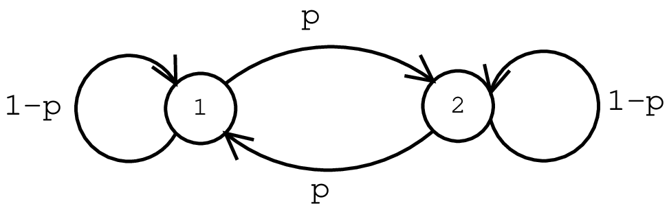
The states are labeled 0 and 1, and we start in state 0. We switch states with probability , and remain in the same state with probability . If , then the probability of being in state 0 is . But if , then . Therefore, is discontinuous at . If we want to prove general smoothness results, we’d better avoid cases like this one.
It will be very useful to consider a strong type of monotonicity from which we can deduce various other smoothness and monotonicity results.
Definition 5.1.70 (D).
A function is absolutely monotonic (D) in iff it has derivatives of all orders that satisfy
Let and , for .
Definition 5.1.71 ().
A function is absolutely monotonic () in iff
| (5.1) |
for all non-negative integers and for all and such that
Absolute monotonicity is useful because of the following facts:
Theorem 5.1.72.
Moreover, if is absolutely monotonic in , then is analytic on . In fact, can be analytically continued on an open disk of radius centered at (so the Taylor expansion of at converges inside this disk).
Proof 5.1.73.
A slight change in a paper by Zazanis [48] allows us to get our first interesting conclusion.
Theorem 5.1.74 (Zazanis).
Suppose we have a discrete time queueing system where exogenous packets are inserted to classes according to a rate Bernoulli arrival processes. Suppose that the system is ergodic if . Then the expected queue length and the stationary probabilities for any state are analytic functions on .
Proof 5.1.75.
Zazanis [48] proves this result in continuous time for Poisson arrivals. His proof amounts to showing that a particular function is absolutely monotonic, and hence analytic. He begins his Theorem 3 with his Equation (1):
(A derivation of this formula, which Zazanis merely quotes, can be found in Brémaud [10], particularly pages 190-191.) The discrete time analogue (where replaces ) is
| (5.2) |
The rest of the changes to Zazanis’ proof follow immediately from replacing his equation 1 with Equation 5.2 above.
A special case is, of course, a Bernoulli ring:
Corollary 5.1.76.
For any fixed , the expected queue length per node of a standard Bernoulli ring is an analytic function of on . The stationary probability of being in any fixed state is also an analytic function of on the same interval.
5.2 Light Traffic Limits
Note that the functions in Theorem 5.1.74 are analytic at . This means that the Taylor expansion around is well-defined and agrees with the actual function in some -neighborhood. Calculations taken in the limit as are sometimes called light traffic limits. Theorem 5.1.74 shows that for Bernoulli arrivals, the light traffic limits are well defined.
5.2.1 Product Form Results
We can use these light traffic limits to prove that certain stationary distributions are not product form, answering a question posed in Section 2.9
Theorem 5.2.78.
For , the stationary distribution of a standard Bernoulli ring is product form. For , the stationary distribution is not product form.
Proof 5.2.79.
Chapter 4 shows the existence of stationary distributions for all when the nominal load . The results of Chapter 2 showed that the stationary distribution is product form for .
Assume that . I will continue to use the state notation of Chapter 2, where
represents a node with packets in queue, and a hot potato with steps left to travel (so ). An empty node (no packets in queue, and no hot potato packet in the ring) is represented as
Imagine that packets travel from left to right.
Consider the state where all nodes are empty except for two adjacent nodes:
The stationary distribution of can be Taylor expanded around zero in the form:
Define to be the ground state, where every node is in state .
In Theorem E.1.200, I show that in order to calculate , we only need to consider contributions from states that are reachable from by inserting at most packets. Since it takes two packet arrivals to get to from the ground state, then . Let’s figure out what terms contribute to .
We can calculate the stationary probability of by adding the stationary probabilities flowing in to it. However, since we’re only going to look at terms of order and lower, then we need only look at states that are attainable with two or fewer packets:
(By , I mean that the and lower terms of the Taylor expansion are equal.) Let be the result of reversing , i.e. all nodes are empty except for two adjacent nodes:
If we consider the possible prior states reachable with two or fewer packet arrivals, there is no analogue of the state, i.e.
(This asymmetry is due to the fact that three packet arrivals are necessary to get to a state like .)
Note that the term in is , which is non-zero. Now, assume for a moment that the distribution were product form. Then the first three terms on the right hand side of Equation would equal the three terms on the right hand side of Equation . Since the term in is nonzero, it follows that the term in is different from the term in . Because these are analytic functions of at , it follows that , except at a finite number of points. This fact contradicts the assumption that the distribution was product form.
Another interesting family of rings are the geometric rings of Coffman et alia [14], [15]. (The following theorem doesn’t use light traffic limits, but it makes a nice counterpoint to Theorem 5.2.78.)
Theorem 5.2.80.
Fix , such that . Suppose for any , we have an -node ring where a packet arrives at each node with probability , and departs on each step it travels with probability . Then there are only finitely many such that the node ring has a product form stationary distribution.
Proof 5.2.81.
Suppose not. Let us restrict our attention to the infinitely many with product form stationary distributions. Then the probability of the ground state (where all the nodes are empty) is the sum of all the stationary probability flowing in to it. A state preceding has packets travelling in the ring and no packets in queue, and becomes state with probability
Let be the marginal probability that a node is empty, and be the marginal probability that a node has one packet (travelling in the ring) in it. Then by the product form,
and by applying the product form to the possible previous states,
Taking the th root and simplifying, we get
The nominal load at any node is . Now, by Little’s theorem (Theorem A.5.152), . Therefore,
If we take the limit of large , we get
Next, observe that the expected queue length per processor is greater than the probability the queue is non-empty. In the limit of large , the probability of a non-empty queue becomes
Therefore, the expected queue length has an lower bound in . However, Coffman et al. [14] shows that the expected queue length is , which is a contradiction.
5.2.2 Explicit Calculations
Suppose we perform a Taylor expansion in at . Since every packet insertion into the ring is one of equally likely possibilities, then the coefficients of the Taylor expansion in are integral. With some care, it’s possible to write computer programs to calculate these coefficients exactly, since there are no rounding issues. (I discuss the details in Appendix E.) I include two such calculations for the node standard Bernoulli ring.
The expected queue length per node, for the first 18 coefficients, is:
| (5.8) |
The stationary probability of all the nodes being empty is:
| (5.9) |
We can deduce a few facts from these enormous polynomials.
Theorem 5.2.82.
The expected queue length per node of the standard Bernoulli ring is not always absolutely monotonic.
Proof 5.2.83.
If , then the expected queue length is absolutely monotonic. However, if , then observe that the term in Equation 5.8 is negative, contradicting absolute monotonicity.
As we’ll see in the next section, Markovian networks have absolutely monotonic expected queue lengths, so Theorem 5.2.82 disproves a natural hypothesis on standard Bernoulli rings.
Next, we analyze the rationality of these functions.
Definition 5.2.84.
Given a rational function , where is an degree polynomial, and is a degree polynomial, define the degree of as .
Theorem 5.2.85.
Proof 5.2.86.
Suppose that we have a partial Taylor expansion of a rational function, something like:
(Or, telegraphically, . For notational simplicity, I interpret if or , or if .) Now, if is too small relative to and , we have no hope of reconstructing or ; in other words, for a fixed , we can only detect rationality if we assume that and are sufficiently small. So, suppose that . Consider the coefficient of . It’s
We can perform a similar operation for the coefficient for the term, and so on, up to . We get a resulting matrix equation:
So, given , we can construct the matrix for any . If the resulting matrix doesn’t have an annihilating vector (i.e. is of full rank), then can not be a rational function with numerator degree and denominator degree . I checked the resulting matrices for Equations 5.8 and 5.9 for all exhaustively11 1 And exhaustingly. via computer, and found that every matrix had full rank.
(A computational note: it is sufficient to reduce the matrix modulo a large prime and show that the resulting matrix is nonsingular by modular arithmetic.)
Finally, the curious reader may wonder what the first few places of the Taylor expansion of the expected queue length per node looks like as a function of . It is possible to calculate these values, and it begins:
or, in terms of the nominal load ,
Observe that the coefficient to is , as one might suspect. The proof can be extended to the term, but even the calculations for the term are too lengthy to include here.
5.3 A Class of Absolutely Monotonic Networks
We now turn our attention from multiclass networks to simpler Markovian networks. First, we need a little combinatorial result.
Lemma 5.3.87.
If , then
| (5.10) |
Proof 5.3.88.
Suppose we have distinct objects which we are allowed to paint red, green, or blue. We have the restriction that of the objects must be red, and we weight each combination by where of the objects are green. Then observe that the weighted sum of all valid combinations of objects is exactly Equation 5.10.
I will prove the theorem by induction on . Observe that the theorem holds if (and hence ).
Assume, inductively, that the theorem holds on . Suppose that . We can sum all the weighted objects as follows. If the last object is red, then there must be red objects among the other objects. If the last object is green or blue, there must be red objects among the other objects. If it’s green, though, we also must invert the weight of the combination. In equations,
By induction,
If , then the last object can’t be red, so the equations simplify:
By induction,
and we are done.
Next, I’m going to define a discrete version of a Taylor expansion, and use Lemma 5.3.87 to find another method of proving absolute monotonicity.
Let be a function on that we suspect may be absolutely monotonic. Fix , an integer, such that . Let .
- •
Let . (So is a constant function defined on .)
- •
For , let
(5.16)
We can now prove the following lemma.
Lemma 5.3.89.
The function is absolutely monotonic iff for all as above.
Proof 5.3.90.
Observe that if , then
So, if we plug into Equation 5.1, we get
For a fixed , the term is independent of , so
By Lemma 5.3.87, when , each of the terms of the second sum is equal to zero. Since if ,
Therefore, the problem of showing that is equivalent to showing that .
We are now ready to prove our main result about Markovian networks.
Theorem 5.3.91.
Suppose we have a (discrete time) Markovian network with nodes, where each node has a Bernoulli arrival process of rate .
Suppose that if , then the maximum nominal load at a node is less than one. Then the network is stable for , and the expected time that a packet spends in the system is an absolutely monotonic function of , for .
Proof 5.3.92.
The stability is immediate because the network is Markovian; see the discrete time fluid limits from Chapter 4 of this thesis, and Section 5 of Dai [20].
Let be the expected delay in the system when the arrival rate is . Define as in Equation 5.16.
I’ll use what is sometimes called the “method of collective marks” (see, e.g. Kleinrock [34], Chapter 7). We want to compare with . We need very fine control over our Bernoulli arrival process. We will get this control as follows.
Let . Let , and generally, . (Note that the are disjoint.) On each time step, at each node, we select a number from uniformly at random. Suppose that we inject a packet if . Then we have simulated a rate Bernoulli arrival process.
If a packet arrives because , let us mark it with an (hence the name “collective marks”.) The packets are now members of class . Suppose that we give priority to packets based on their mark, so that packets with lower marks get priority over packets with higher marks.
The key observations to make are twofold. First, since the mark packets have priority over all the other packets, they behave as though they were travelling in a system with a rate Bernoulli arrival processes. Therefore, the expected delay of the mark packets is the same as the expected delay from a rate Bernoulli process, namely .
Second of all, the increase in expected delays from inserting multiple classes of marked packets is superadditive. To clarify this point, let me give a canonical example (with ). Suppose that we compare the system with arrivals when
- 1.
,
- 2.
,
- 3.
, or
- 4.
,
where . Let us call the expected delay in the systems , , and , respectively.
In both cases 2 and 3, we have Bernoulli arrival processes of with the same rate. Therefore, . In particular, the increase in expected delay from cases 1 to 2, and from cases 1 to 3 is identical. In the fourth case, the class packets will be delayed by the class 0 packets, and additionally delayed by the class packets. Therefore,
To see more formally why the delay is superadditive (i.e. that the increase from to is at least ), let us examine the packets’ paths a little more closely. Whenever a packet is ejected from a node, it selects its outgoing edge based on some distribution. Let us fix these decisions ahead of time, per class, rather than dynamically as the system runs. That is, at start up we decide that the th packet that is marked at node will take edge , for all , and . (If no edge is selected for some , then the packet must leave the system.)
Let us compare the system with the class and class packets, versus the system with only the class packets. I claim that the th class packet ejected from node will be ejected at the same time or later in the system than in the system. The proof follows immediately by induction on time. (This technique was introduced by Harchol-Balter [31].) Clearly, if the system departures for the class packets occur no sooner in the system than in the system, then the expected delay of class packets in the former system is at least as great as in the latter system. In other words, the delays are superadditive.
Now, let us consider . The addition of an additional class of marked packets can only increase the total expected delay. Therefore, if the arrival rate is , with , then
and hence,
Next, consider . Suppose we let be the expected delay from arrivals caused by , and by arrivals caused by alone, for . There are such arrival processes. First of all, the increase in delay that each of these processes offers over the process is identical. Second of all, if we consider the arrival process , we can simply add all the differences (because the delays are superadditive.) Now, and , for any , so
| (5.17) |
How do we show that this process continues for , for arbitrarily large ? Well, we know that if , then
| (5.18) |
Suppose, in addition, that for any ,
| (5.19) |
hence
We will prove Equation 5.19 by induction on . We’ve already proved the base case (). Assume it holds for all .
As discussed in the case, the delay in packets from is greater than the sum of
- •
The delay in the packets arriving because .
- •
The increase in delay caused by the packets arriving in , for . There are such sets.
- •
The increase in delay caused by the packets arriving in , for . There are such sets.
- •
….
- •
The increase in delay caused by the packets arriving in , for . There are such sets.
where and . This sum is precisely equal to
So, since is an upper bound,
giving Equation 5.19 as desired.
If we look at the preceding proof a bit more carefully, it is possible to show that the expected delay is strictly increasing and strictly convex. We will deduce some more interesting corollaries on expected queue lengths below.
Corollary 5.3.93.
Suppose that we have a Markovian network with Bernoulli arrivals of rate , with nominal loads less than one so long as . Then the expected number of packets in the system is absolutely monotonic, as is the expected (total) number of packets in queue.
Proof 5.3.94.
The expected delay in the system is equal to the sum of the expected delay at each node. By Little’s Theorem (Theorem A.5.152), the expected number of packets per node is the expected delay per node multiplied by . Since every packet has a rate Bernoulli arrival process, the expected number of packets in the whole system is times the expected delay. Multiplying an absolutely monotonic function by retains absolute monotonicity, so we’re done with the first half of the corollary.
Let be the expected total number of packets in queue as a function of , and be the expected total number of packets in the system as a function of .
Little’s Theorem also tells us that if a system is stable, then expected queue length at a node differs from the expected number of packets at that node by exactly the nominal load . Therefore, by the linearity of expectation, equals plus the sum of the nominal loads.
The sum of the nominal loads are a linear multiple of , say . Observe that is an analytic function. Since absolute monotonicity implies analyticity, then is analytic. Therefore, is the difference between two analytic functions, and hence analytic.
Consider a Taylor expansion of around zero. The only coefficient that differs from (and hence the only coefficient that could be negative) is the term. If this coefficient were negative, then for a sufficiently small , would be negative. However, the is always non-negative (since it measures a non-negative quantity.) Therefore, the coefficient is non-negative, and hence is absolutely monotonic.
.
Because an node ring is symmetric, is possible to translate from expected total queue length to expected queue length per node; we simply divide by . This fact gives us a final corollary:
Corollary 5.3.95.
A geometric Bernoulli ring is Markovian, and hence its expected queue length per node is absolutely monotonic.
5.4 Future Work
Suppose we have a family of Markovian networks with Bernoulli arrivals, , for . Suppose is the expected number of packets in queue in network when the nominal load is (this presupposes some notion of a system-wide nominal load; for instance, the maximum nominal load on any node.) From the results of the previous section, we know that is absolutely monotonic for .
Suppose, finally, that for any , there exists such that . Then there exists a function absolutely monotonic on and a subsequence such that
Now, since the are absolutely monotonic, it implies they are monotonically increasing and convex, and hence that is also monotonically increasing and convex. Convexity implies continuity on open intervals (see Rudin [43], page 61), giving continuity on . The monotonicity allows us to extend the continuity to . By Dai’s [20] Lemma 4.1, the converge uniformly on compact sets, so it follows that is analytic, and the Taylor coefficients are the limits of the coefficients of the . Therefore, is absolutely monotonic.
Now, recall the known bounds for a standard Bernoulli ring:
- •
If , then is .
- •
If , then is .
Suppose that the standard Bernoulli ring were absolutely monotonic. Then the arguments above would let us conclude that the expected queue length converges to an analytic function , which is identically zero on , and is analytic on . By analytic continuation, it follows that is zero on the whole interval , i.e. the expected queue length per node would be !
Sadly, these arguments don’t work. A standard Bernoulli ring is not Markovian, so Theorem 5.3.91 doesn’t apply; in fact, as we showed in Theorem 5.2.82, there exist for which the node standard Bernoulli ring is provably not absolutely monotonic. However, an interesting avenue of future research would be to find some smoothness property analogous to absolute monotonicity. Using it, we might be able to make conclusions about based solely on analytic continuation arguments.
Chapter 6 Ringlike Networks
6.1 Introduction
A ring is the simplest possible network with feedback. If we wished to generalize results about the ring to other networks, where should we begin?
One way of characterizing a ring is to observe that it is a regular degree 1 directed graph where all nodes are identical. (By identical, I mean that there exists a graph automorphism that sends any node to any other node. This property allows us to calculate the expected queue length per node simply by dividing the total expected queue length by .) A natural first step in generalization is to increase the degree of the graph, but maintain regularity. I will discuss two possibilities, the butterfly and the torus. First, though, I will define a more general class of networks, of which butterflies and tori are members.
Definition 6.1.96.
A directed graph is layered if its nodes can be partitioned into disjoint sets such that any edge lies between and for some . A layered network is also called feedforward.
A wrapped layered network allows edges from to , too.
Now, to define the two graphs of interest:
Definition 6.1.97.
A torus is a directed graph consisting of nodes. A node is labeled , where is an integer between and . There is an edge from to iff there is an such that , and for all , .
If for all , the torus is called a -dimensional hypercube.
If divides for all , then the torus can be written as a wrapped layered network with layers.
Another popular network for packet routing is the butterfly graph.
Definition 6.1.98.
A (standard) -dimensional butterfly is a directed, layered graph defined as follows: nodes fall into one of disjoint layers, numbered 0 through . Each layer consists of nodes, which we label with the binary strings of length . (So, a node is specified by a binary string and a layer number.) Consider any length binary string, say . For each such that , there is a directed edge from node of layer to node of layer , and another directed edge from node of layer to node of layer . The nodes on layer 0 are called the input nodes, and the nodes on layer are the output nodes.
A wrapped butterfly is a directed graph where the nodes on the last layer are associated with the nodes on the first layer.
See Figure 6.1 for a drawing of a three-dimensional butterfly graph.
includegraphics[height=2in]figures/butterfly3.eps
Note that tori and wrapped butterflies are both regular layered graphs where every node is identical.
It will be useful to keep these examples in mind during the next section.
6.2 Convex Routing
Definition 6.2.99.
Consider a node in a network. Let be the nodes with directed edges into . Let be the probability that a packet travels from node to , and suppose that the probability is independent of the class of the packet.
Suppose that
| (6.1) |
If this equation holds for all nodes , then we say that the network11 1 Is convex routing a property of the network or of the protocol? Although some may take issue with me, I view the selection of edges as a function of the packet class, determined by the network. The protocol, on the other hand, selects which packet gets ejected, not where it goes. has the property of convex routing.
For example, if we are on a regular graph, and a packet chooses its next edge uniformly at random, the network has convex routing.
Theorem 6.2.100.
Suppose we have a generalized Kelly network with convex routing. Suppose further that we use any greedy protocol, and the network has any topology. If the nominal loads are less than one, then the network is stable.
If all the interarrival and service times have finite variance, then the expected queue length is finite, too.
Proof 6.2.101.
I’ll prove this by using the (delayed) fluid limit technique.
Let be a node. I’m going to define a potential function on the fluid model to be the analogue of the expected congestion at node (i.e. the expected number of times that packets now in the system will use node ).
To make this precise in the fluid regime, consider a fluid class and a node . Suppose that we have a unit of class fluid, and suppose that class resides at node . Suppose we have a path through the network (not necessarily node disjoint), beginning at class ’s node and ending at node . Then some fraction will pass through node along path . (Note that is independent of the class by the convexity of the routing.) Since we have an open queueing network, all packets almost surely leave the system. In the fluid domain, this means that, summing over all paths from to ,
Suppose that there is quantity of fluid of class . Then, since there are a finite number of classes , we can let
Notice that is the total amount of fluid that would pass through node if no new fluid arrived in the system. Let .
Let be the number of packets in queue at node (from all classes resident at ). Let be the nominal arrival rate at node . Let be the nominal service rate at node . (Note that , since the nominal loads are less than one.) Let
Observe that is a Lipschitz function. To see this, note that fluid increases at most at a rate , and decreases at most at a rate . It follows that is Lipschitz.
Now, Lipschitz functions are absolutely continuous, and hence continuous and differentiable almost everywhere. (See, e.g., Rudin [43]). If we can show that implies that a.e., then it implies fluid stability (because all fluid will empty from the system by time ), and we will be done.
Observe that if , then
almost surely. Therefore, if the maximum value of is attained at a node with , then it follows almost surely that .
It suffices, therefore, to show that so long as there exists an with , then
| (6.2) |
and we will have proved fluid stability.
Assume that . If for all , then Equation 6.2 holds. Assume, then, that there exists a node such that , but .
I am going to construct a tree of all the possible paths from node with to node , where every intermediate node on the path has . Since but , then there must exist some such path, so the tree has more than one node.
It’s certainly possible that by the third level of the tree, a node from the network may show up in more than one place in the tree, because there may be multiple paths from the node to . We treat these as formally distinct nodes. (For instance, if we have a diamond shape, as in Figure 6.2, node from the network will split into two different nodes in the tree.)

The terminal nodes in the tree correspond to nodes in the network with non-zero queues. I will label the terminal nodes to represent the amount of traffic that will follow a given path. More precisely, consider a node in the tree, corresponding to node in the network, and the path from to . Let be the class of paths that start at the node where class packets are located and end with . Then define
If is a terminal node in the tree, I will label it with .
Now, let be the set of terminal nodes in the tree. Observe that
| (6.3) |
Consider taking a random walk along the tree away from the root node. Given the edges leading to node , let the probability of crossing edge in our random walk be the probability of crossing the edge into node . Because the routing is convex, the sum of the probabilities is
If , then with probability , we stop the walk in node . Observe that for any terminal node , the probability of stopping at node is . Since we have a distribution,
| (6.4) |
(This inequality can also be proved from the Kraft inequality of data compression theory.)
Equations 6.4 and 6.3 combine to tell us that is bounded by a convex combination of the terminal nodes.
Note that if we have a convex combination of non-negative reals that are all less than some bound , then there exists an such that the convex combination is less than or equal to . Using the total work in the system as a bound on , we can conclude that
| (6.5) |
for some particular node .
Finally, observe that if node in the network corresponds to terminal node in the tree, then (at least) packets currently in the system need to cross . Therefore,
| (6.6) |
Combining Equations 6.5 and 6.6, we get
Note that node has (because is a terminal node of the tree), so we have established fluid stability.
Fluid stability, plus the finite variance of arrivals and service times, implies finiteness of expected queue length. (For details, see Dai and Meyn [23]).
Corollary 6.2.102.
Any ring network uses convex routing, and thus is universally stable.
Note 6.2.103.
The fluid stability of the ring was first proved by Dai and Weiss [22].
These results on convex routing have some fairly natural applications to load balancing. Suppose we have a -dimensional wrapped butterfly where each nodes is a processor, performing some computations. Occasionally, a node will decide that it has too much work, and will insert a packet into the system, representing one quantum of work. The processor would like to share its work fairly uniformly across the other processors. (For the moment, I won’t worry about aggregating the completed work of the system.)
Sharing the load can be accomplished fairly easily on a wrapped butterfly. At every node, there are two outgoing edges; if a packet selects each edge with probability , then in (or more) steps, its probability of being at any point in its current layer is uniform. Thus, we have a multi-class convex routing problem, and we can use Theorem 6.2.100 to deduce stability.
There is an even more efficient method of sending the load through the network. Since there are two outgoing edges at every node, we can send out up to two packets per time step. Suppose that we select the particular edge at random. Then we maintain convex routing (and hence stability), while still guaranteeing uniform distribution over the final layer in time steps.
Generally speaking, if we have a -regular graph, then by selecting each of the outgoing edges with equal probability, we have convex routing. We can also send out packets instead of 1 packet. Most interestingly, since at most packets arrive, we can give them precedence over the packets in queue, i.e. use the Greedy Hot Potato algorithm. This choice opens up the possibility of using the techniques from Chapter 3 to get bounds on the expected queue length per node.
6.3 Superconcentration on a Pair of Butterflies
The remainder of this chapter will examine some problems in node-disjoint circuit switching. Unlike the stochastic results of the rest of this thesis, these results are more graph-theoretical and structural in flavor. The motivating problem can be described as follows. Suppose we have a directed graph with input and output nodes, both labelled from 1 to . For each input node , we choose an output node to be its destination, for some permutation . The problem is to find a collection of node-disjoint paths which each run from to for all . A directed graph that can route all permutations is called rearrangeable. (For some real-world applications of node-disjoint routing, see, for example, [47].)
A classic example of rearrangeability is the Beneš network (see [36]). This network (i.e. directed graph) consists of a “forward” butterfly adjoined to a “reversed” butterfly. A natural question to ask is: if we attach two “forward” butterflies, is this network (the double butterfly) still rearrangeable? This problem has been open for several decades. At least one proof is currently under review [11]. This suggests a more general hypothesis. Suppose that we have two graphs, each isomorphic to a butterfly, but not necessarily identical to each other. If we attach the output nodes of the first to the input nodes of the second, is the resulting graph rearrangeable?
At the current time, proving this kind of result seems far too much to hope for. So, rather than show that these types of networks are rearrangeable, I will prove various concentration and superconcentration results.
Definition 6.3.104.
Consider a directed graph . Fix input nodes and output nodes. Suppose that between any input and output nodes there exist node-disjoint paths. (By “node-disjoint”, I mean that a path intersects neither itself nor any other path.) Then we say that is a -concentrator. If is a -concentrator for all , then we call a superconcentrator.
(Observe that every selected input and output node occurs on exactly one path. Note also that node-disjointness implies edge-disjointness of the paths. See [41] or [32] for more on superconcentrators.)
Clearly, rearrangeability implies subset routing– just choose a permutation that respects iff . However, the converse is not true for arbitrary networks (see Figure 6.3).

It’s straightforward to show that a single butterfly does not route all subsets, so we need to use at least two butterflies to get interesting concentration results.
In the next several sections, I show that any concatenated pair of -dimensional butterflies (not necessarily identical to each other) are -concentrators, for any . I can strengthen this statement in a special case: if the butterflies are standard butterflies with their layers shuffled (e.g. a Beneš network, or the double buttefly in [11]), the network is a superconcentrator.
The rest of this chapter is structured as follows. Section 1 establishes some definitions and fixes notation. Section 2 examines the structure of a graph related to a pair of butterflies that highlights some of its connectivity properties. Section 3 solves the problem in the case where for some , and proves a rearrangeability-type result when on certain networks. Section 4 presents the main result, except for one lemma that I postpone for section 5. Section 6 is dedicated to closing remarks.
6.4 Definitions and Notation
Let us begin by defining and fixing notation for a butterfly. A standard -dimensional butterfly can be viewed as a network with nodes where we switch the first bit in the first layer of edges, the second bit in the second layer of edges, and so forth. If we choose to switch the bits in a different order, we get a layer-permuted butterfly.
Definition 6.4.105.
A -dimensional layer-permuted butterfly is a directed, layered graph defined as follows: nodes fall into one of disjoint layers, numbered 0 through . Each layer consists of nodes, which we label with the binary strings of length . Take some (fixed) permutation on objects. Consider any such binary string, say . For each such that , there is a directed edge from node of layer to node of layer , and another directed edge from node of layer to node of layer .
(Note that these butterflies are all graph-isomorphic to each other.) Finally, the networks we’ll be looking at consist of pairs of these butterflies.
Definition 6.4.106.
Suppose that we have two graphs, and . Suppose that has output nodes and has input nodes, each numbered from 1 to . Then we say that is the concatenation of and if we form by associating the output node of with the input node of .
If and are each isomorphic to a standard butterfly (but not necessarily identical to each other), we call a pair of butterflies. Similarly, if and are layer-permuted butterflies, we have a pair of layer-permuted butterflies. Finally, if and are both standard butterflies, we have a double butterfly.
Note that these graphs have layers of nodes (0 through ). Since I imagine the paths from inputs to outputs to be running from left to right, I will refer to the butterfly on layers 0 through as the left butterfly, and the one on layers through as the right butterfly. Note also an alternate way of specifying a pair of butterflies: consider a network consisting of two standard butterflies, but permute the labels of the output nodes of the left butterfly. Observe that these two definitions give rise to the same class of graphs (up to isomorphism).
Over the course of this chapter, I construct directed node-disjoint paths from input nodes to output nodes. So, for example, a path from an input node to an output node on a pair of butterflies is exactly nodes long– the path can’t double back on the layers.
Suppose I have a set of input nodes and a set of output nodes of the same size (i.e. ) Then if I specify a collection of node-disjoint paths from to , observe that I can extend these paths into a consistent setting of all the switches in the network. These switches will induce node disjoint paths from every input to every output node, and retain the feature that a path begins in iff it ends in . So, on a switching network, node-disjoint routing of a subset implies there exists a node-disjoint routing of a permutation such that iff . Since this is an “if and only if” statement, we get the following lemma:
Lemma 6.4.107.
If we can find node-disjoint paths from to on a switching network, then we can find node-disjoint paths from the complements to .
Throughout this chapter, I will use to represent a collection of input nodes, a collection of output nodes, and assume that .
6.5 The Sub-Butterfly Connectivity Graph
Suppose we specify a path of length on a standard butterfly (for ) from an input node. By choosing which edge to take, the path changes bits of its location any way we want. Suppose we select the first bits to be . Then from layers to , the first bits will remain equal to . Let’s specify the resulting sub-graph of the butterfly in the following definition:
Definition 6.5.108.
Consider a dimensional standard butterfly. Take an bit binary string (). Consider the sub-graph formed by the nodes on layers through (inclusive) whose first bits are . Observe that this graph is (isomorphic to) a -dimensional butterfly. Let us call it the sub-butterfly .
If we specify a suffix instead and consider layers 0 through , we get the sub-butterfly .
If we have a graph isomorphic to a standard butterfly, the isomorphism will induce (isomorphic) images of the sub-butterfly, so we can meaningfully refer to sub-butterflies on any butterfly-isomorphic graph.
I will be considering sub-butterflies in a pair of butterflies. In this context, is the sub-butterfly residing on layers through (and stopping there), i.e. only in the left butterfly. I’ll also be interested in sub-butterflies on the right side. These inhabit layers through .
It will be useful to investigate the structure of the connections between the -dimensional sub-butterflies on the right and left sides of a -dimensional pair of butterflies, that is, the sub-butterflies of the form or where is a binary string of length (such that ). Note that these sub-butterflies inhabit layers through , and through . Let us represent each sub-butterfly by a vertex in a bipartite graph; the vertex is on the left side of the bipartite graph iff the sub-butterfly is on the left side of the pair of butterflies. I will label each vertex by its associated sub-butterfly, abusing the label notation somewhat. Place an edge between two vertices and iff the two sub-butterflies are connected, that is, iff and (as sub-butterflies) share at least one common node on layer of the pair of butterflies. Equivalently, there is an edge between the nodes in the bipartite graph iff there exists a path from every layer input node of to every layer output node of . I will refer to this graph as the -dimensional sub-butterfly connectivity graph, or just the connectivity graph. Observe that there are vertices on either side of this graph. How are the vertices connected?
I will consider progressively more specialized cases in order to derive various results in later sections. Suppose, first, that we build a bipartite connectivity graph, but if there are common nodes on layer between a sub-butterfly on the left and one on the right, we insert edges (instead of only 1 edge). Let us call this the enriched connectivity graph.
Lemma 6.5.109.
For any pair of butterflies, its enriched connectivity graph is regular.
Proof 6.5.110.
Since each sub-butterfly has output nodes, then all nodes in the enriched connectivity graph have degree .
Now we move our attention to the special case of layer-permuted butterflies. First, let us analyze the structure of one connected compnent of the -dimensional connectivity graph.
Lemma 6.5.111.
Each connected component in the connectivity graph of a layer-permuted butterfly is a completely connected bipartite graph.
Proof 6.5.112.
Suppose that the layer-permuted butterfly on the left has permutation , and the butterfly on the right has permutation . Consider a sub-butterfly in the left butterfly. This corresponds to a sub-graph on layers through where the value of bit is . Notice that a sub-butterfly in the left butterfly connects to a sub-butterfly in the right butterfly if and only if
| (6.7) |
Thus, each connected component is a complete bipartite graph (with the same number of nodes on each side.)
Next, suppose that we have a pair of layer-permuted butterflies. How does the graph change as we specify one more layer? That is, if we compare the connectivity graphs between and dimensional sub-butterflies, what happens?
Therefore, determining the structure of the connectivity graph on pairs of layer-permuted butterflies reduces to determining the connected components. Consider one connected component in the connectivity graph looking at -dimensional sub-butterflies. When we advance to the dimensional sub-butterflies, each node becomes two nodes (because each dimensional sub-butterfly splits into two dimensional sub-butterflies). There are essentially three cases that can occur.
- •
(No reused dimensions) Suppose that for any and for any . Then if the -dimensional sub-butterfly is adjacent to , it follows that is adjacent to for .
In the connectivity graph, that means that the connected component doubles the number of nodes, but remains completely connected.
- •
(One reused dimension) Suppose that there exists (exactly) one such that either
- –
, or
- –
for some and for any , or
- –
for any and for some
Then the connected component splits into two connected components, based on the value of the th bit.
- –
- •
(Two reused dimensions) Suppose that for and for , and . Then the connected component splits into four connected components, based on the four possible values that the and bits can take.
6.6 Subsets of Size
We want to select a collection of node-disjoint paths from input set to output set on a pair of butterflies. Although I’ve expressed this problem in terms of paths, it’s often easier to express the proof in terms of packets travelling through the network. In particular, if packets travel forward (node disjointly, and without stopping) from every input node in , and backwards from every output node in , and we can match up the packets on level , then the paths traced by the packets give us the collection of paths we’re looking for. I will switch between the path and packet descriptions of the problem whenever it seems helpful.
Lemma 6.6.113.
Suppose we have a set of input nodes on a butterfly. By passing from layer 0 to layer 1 of a butterfly, there exist paths that send of the packets to sub-butterfly , and of the packets to sub-butterfly . Similarly, we could send of the packets to sub-butterfly , and of the packets to sub-butterfly . Mutatis mutandi, this applies to packets in output nodes travelling backwards, by passing from layer to .
Proof 6.6.114.
The nodes on the first layer of the butterfly can be grouped into switches, where the nodes labelled and form one switch. Observe that each switch can be set straight or crossed, that is, we have to send to on the next layer (for both 0 and 1), or to . Setting switches in one of these two states guarantees that paths are node-disjoint, so I will always set them accordingly.
For all the switches such that , half of these packets get sent to , and half to . If , half of these (zero) packets get sent to each sub-butterfly, too. Consider all of the remaining packets. Each of these is the sole packet in the switch. So, by setting of the switches to send the packets to sub-butterfly , and of them to , we prove the first part of the lemma. The rest follows by symmetry.
This lemma allows a surprisingly simple proof of concentration.
Theorem 6.6.115.
Suppose . Then there exist node-disjoint paths from any input set to any output set on a pair of butterflies. (In other words, a pair of butterflies is a -concentrator.)
Proof 6.6.116.
Consider the left butterfly. We can apply Lemma 6.6.113 recursively for steps. On step 1, we split so that packets go to and go to . Since and are themselves dimensional butterflies, we can apply the lemma again, on each of them, giving us 4 sub-butterflies, each with paths. After steps, we end up with sub-butterflies (which is all of the dimensional sub-butterflies), each of which has exactly 1 packet. Now, on each of these butterflies, we can send the packet along any path we want for the remainder of the left butterfly (i.e. until we hit layer ); since it’s the only packet on its sub-butterfly, there’s no possibility of any other packet’s path crossing its own.
We can perform the same construction on the output packets in , moving backwards toward the input layer. When we reach layer , there will be 1 packet per sub-butterfly.
At this point, observe that the sub-butterfly connectivity graph determines the connections between these butterflies. By Lemma 6.5.109, this graph is a regular bipartite graph. By Hall’s theorem, there exists a perfect matching. This matching in the connectivity graph implies a matching in the set of sub-butterflies, which implies a matching between the (unique) packets in each sub-butterfly. By construction of the connectivity graph, there exists a path (not necessarily unique) between matched packets. As observed above, these paths are node-disjoint, so we’re done.
6.6.1 Some Corollaries
We get a very short corollary:
Corollary 6.6.117.
Suppose . Then there exist node-disjoint paths from to on a pair of butterflies.
We can use Theorem 6.6.115 to give us information about a kind of rearrangeability on sufficiently small input and output sets.
Corollary 6.6.119.
Suppose we have a pair of -dimensional butterflies. Suppose that there is a path between each node on layer (in the left butterfly) and each node on layer (in the right butterfly). Then if we select any input set and output set with , and any permutation from to , there exists a collection of node-disjoint paths from to such that for every , the path from ends at .
Proof 6.6.120.
If the corollary holds when , then, by using dummy packets to make up the difference, the corollary holds for . So, suppose that . We can use the same argument in Theorem 6.6.115 to split the packets until there is one packet on each dimensional sub-butterfly. By the assumption in the corollary, the resulting connectivity graph is a complete bipartite graph on all nodes, so we can select node-disjoint paths between the path originating at any and send it to the path terminating at .
Note that if we have a pair of standard butterflies, the corollary holds. Also, suppose we have a pair of layer-permuted butterflies. Suppose further that we insist that
- •
if , then (where is the left layer permutation) on the left butterfly, and
- •
if , then (where is the right layer permutation) on the right butterfly.
(In other words, we permute the layers but don’t send any layer from the left half of the butterfly to the right half.) Then Corollary 6.6.119 holds.
6.7 The General Case
Proving node-disjoint subset routing for an arbitrary input and output set (of the same size) is somewhat more challenging. However, for pairs of layer-permuted butterflies, the same basic approach from Theorem 6.6.115 works. Looking at the proof, there are two parts: first, we split the packets into a number of sub-butterflies, until we have one packet per sub-butterfly. Then, we view the problem as an exact matching problem on a particular bipartite graph, and show that a matching exists.
The proof for the general case runs the same way. In order to find a matching, it’s clearly necessary that each connected component of the bipartite connectivity graph has as many packets on the left side as on the right. In the next section, I’ll prove that this condition (roughly speaking) is sufficient for the existence of a matching on the connectivity graph. But assuming for now that it holds, we can prove the main result:
Theorem 6.7.121.
For any input set and output set on a pair of -dimensional layer-permuted butterflies, such that , there exist node-disjoint paths from to .
Proof 6.7.122.
If , then we are done, by (for example) Theorem 6.6.115. So throughout, we can assume that . Suppose that, in binary, , where . I will prove the lemma by induction on . The exact statement that I will be inducting on is:
Over the course of steps, we can recursively split the packets over the sub-butterflies, so that if sub-butterfly has packets in it, then will have or packets, and will have or packets, respectively. The same holds on the right butterfly. (There will then be 0 or 1 packets in each sub-butterfly on level and level ). We can then select a matching between the sub-butterflies giving us node-disjoint paths from to .
First, the base case: if =0 or 1, then we are done (by Theorem 6.6.115).
Next, the inductive step. Fix and assume the theorem holds for all . Let us try to reproduce the proof of Theorem 6.6.115 with packets to see where complications arise. If , then we will not be able to divide the packets evenly in half at every sub-butterfly for steps. A sub-butterfly may have an odd number of packets, so we must send the “extra” packet either to or . I will refer to this choice (the “0” or “1”) as the rounding decision. Note that there is no actual packet that is distinguished as the “extra” one– there’s just a surplus of one more packet that either goes to or . But it’s helpful to imagine that one of the packets is the extra one when describing the paths.
Choose and such that . Let be the integer such that (so, ). By induction, we can find node-disjoint paths from to . The information that we keep from the induction is not the actual paths themselves. Instead, we keep the rounding decisions that every sub-butterfly makes. Note that even after we’ve split until there’s only 1 packet per sub-butterfly, we are still splitting with an extra packet; it’s just that if , then , and . Hence, the almost exact recursive splitting part of the inductive hypothesis holds not just for the first steps, but for the first steps. We need to keep this rounding information, too.
Consider, now, the original sets and . Using Lemma 6.6.113 recursively for steps on the right and left butterflies, we can send the “extra” packet on each sub-butterfly the same way on level as we did when routing to . To do this, we need to know that the same sub-butterflies have an odd number of packets in them. Observe that if a sub-butterfly on level that has packets in it in the case, then it has in the case. As long as , then and have the same parity; therefore, extra packets exist in the same sub-butterflies. When we reach step , all the -level sub-butterflies that had one packet in them in the case now have 2 packets, and all the sub-butterflies that had no packets now have 1.
We shift now to the matching problem on the sub-butterfly connectivity graph. Consider one connected component of the connectivity graph. Every node on the left hand side represents a sub-butterfly with one or two packets on it, as does every node on the right hand side. By induction, the total number of packets on each side is the same. (If they weren’t, the packets in the case couldn’t match up.) Using Lemma 6.8.123 of the next section, we can split the packets over level (and ) to get 0 or 1 packet per sub-butterfly, with the same number on the LHS and RHS of each of the connected components. By Lemma 6.5.111 each component is completely connected, and we’re done.
Note that since we’re using the direction of the “extra” packet, rather than any particular path, the actual packets going into the upper or lower sub-butterflies are not necessarily the same between the case and the case. In particular, will not necessarily still be routed to .
6.8 The Matching Lemma
Lemma 6.8.123.
Suppose we have a pair of -dimensional layer-permuted butterflies. Consider its -dimensional sub-butterfly connectivity graph, where the sub-butterflies reside on layer , and . Suppose that each node has 1 or 2 packets on it. Finally, assume that there are the same number of packets on the LHS and the RHS of each connected component.
Then, when passing from the -dimensional connectivity graph to the -dimensional connectivity graph, we can send each packet to a different sub-butterfly such that each connected component has the same number of packets on the LHS and the RHS.
Proof 6.8.124.
Since the behavior of the two-packet sub-butterflies is determined (one packet goes to , one to ), this proof will eventually come down to making the correct rounding decision for the sub-butterflies with single packets.
There are three cases we have to consider, reflecting the three possible behaviors of the connectivity graph as outlined on page 6.5.
Case 1: (No reused dimensions) If the connected components don’t split between the and dimensional sub-butterflies, then the lemma is trivially true.
Case 2: (One reused dimension) Suppose that each connected component splits into two connected components. Consider one connected component in the -dimensional connectivity graph that splits into and in the -dimensional connectivity graph.
Suppose that there are nodes in with two packets on them, and nodes with one packet on them. We must send packets to and to on both the left and the right sides because the behavior of two-packet sub-butterflies is determined. We can send the packets from one-packet nodes to either component; we simply send to and to on both the left and the right sides. Then the lemma holds.
Case 3: (Two reused dimensions) Suppose that each connected component in the -dimensional connectivity graph splits into four connected components, e.g. splits into , , , and .
Let us calculate how many of the packets from the 2-packet butterflies arrive in each of these splintered components.
If we have a sub-butterfly on level with 2 packets in it, then we must send exactly 1 packet to and one to . I will refer to these packets as constrained packets. (By contrast, if a sub-butterfly on level has only 1 packet in it, we can send the packet either to or ; such a packet is a free packet.) We shift our view back to the corresponding connectivity graph. Let us label the number of constrained packets on each side of each . Observe first of all that because constrained packets come in pairs, for a fixed or 1, there are as many constrained packets on the LHS of as of , and similarly as many on the RHS of as of . Let the number of packets on the LHS of be , and the number of packets on the LHS of be . Let the number of packets on the RHS of be , and the number of packets on the RHS of be . See Figure 6.4.

Observe that, since each sub-butterfly in layer has either one free or two constrained packets, then the number of packets on the LHS is
Since the analogous equation holds on the RHS, and since the total number of packets are equal, we get that
so there’s the same total number of constrained packets on the RHS and the LHS. Therefore, adding up the constrained packets in Figure 6.4 and dividing by two, we get
Also, any particular or can’t be larger than , so
Due to symmetry, we can assume w.l.o.g. that , , and . Putting this together, we can assume that
Generally speaking, , so there will not be the same number of constrained packets on the RHS and LHS of each connected component of Figure 6.4. However, we still have the free packets to allocate. The situation is as drawn in Figure 6.5.

Since we assume that , then in order to balance the packets on the LHS and RHS, we have to add packets as in Figure 6.6.

We have to show that there are enough free packets to add. There are three inequalities to check. First, for and on the LHS, let us calculate how many free packets are required.
Now, , so we need no more than free packets, which we have. For the other two cases, (namely and ), note that
and in each case, there are free packets. So, in all cases, we can use a subset of the free packets to make the total number of packets on the RHS and LHS equal. Since all the remaining unmatched free packets on the left are connected to all the unmatched free packets on the right, we can choose an exact matching to match these packets, send them to the appropriate connected component, and we’re done.
6.9 Conclusion
Are all pairs of butterflies superconcentrators? Or only the layer-permuted ones? It’s certainly natural to conjecture that the stronger statement is true. As a piece of support, Theorem 6.6.115 can be extended to prove that any pair of butterflies is a concentrator. Unfortunately, the pathological cases (from unusual butterfly isomorphisms) make the general analysis more complicated than I could solve.
The concentration and superconcentration results in this chapter all spring from a splitting and matching approach. This method holds out a tantalizing suggestion of a proof of the rearrangeability of pairs of butterflies. Theorem 6.7.121 can be viewed as follows: if we number each input and output node 0 or 1, and have the same number of zeroes among the inputs and outputs, we can route a permutation that sends and . Suppose we labelled the input and output nodes 0,1,2, or 3, with the same size restraints. The proofs above seem likely to apply to this case, too. If we could just continue doubling the number of labels up to , we’d have proved rearrangeability. Getting the proofs to work for an arbitrary seems pretty challenging, though.
Another natural network to try these methods on is the hypercube. Typically, rearrangeability on the hypercube requires that each edge is used at most once, ever, and concerns edge-disjointness, rather than node-disjointness. A result analogous to Theorem 6.7.121 would be more likely to apply to a hypercube that uses each edge at most once per time step, but possibly multiple times over several time steps. However, edge-disjointness might be strengthened to node-disjointness. Unfortunately, the translation to a hypercube is not trivial.
Proving that a graph is a superconcentrator can also be viewed as a max flow/ min cut problem; thus, Theorem 6.7.121 can be viewed as saying that for any collection of input and output nodes, it is necessary to delete at least edges to prevent any (single-pass) paths from the input to the output sets. One might optimistically hope that these results might translate to other max flow problems, at least on switching networks.
On a possibly more practical note, it’s interesting to observe that the Theorem 6.7.121 makes use of the size of the input set, rather than the set itself (i.e. , not ). It follows that once you calculate the rounding decisions for a particular sized input set, the same rounding decisions solve the problem for all input sets of the same size. This also suggests another method for proving concentration results.
Appendix A Analysis and Probability
A.1 Markov Chains
The most common stochastic object in this thesis is the Markov chain.
Definition A.1.125.
A countable discrete time Markov chain is a stochastic process defined on a countable state space at discrete moments in time . It has the property that the distribution of states at time is independent of the distribution of states at time , conditional on the state at time .
A Markov chain is time independent, if the probability of transfering from state to in one time step is independent of the time .
Suppose that for any pair of states and , there is a nonzero probability of travelling from state to in a finite number of steps, and from to in a finite number of steps. We call such a Markov chainirreducible.
A Markov chain is periodic with period if the number of time steps it takes to get from any node back to itself is always a multiple of , for . A Markov chain is called aperiodic if it is not periodic.
The Markov chains I will be studying will always be irreducible and aperiodic.
The first property of interest in studying Markov chains is their stationary distributions.
Definition A.1.126.
Suppose we have an irreducible, aperiodic discrete time Markov chain with a countable state space. Take any state . Start the Markov chain in state , and let be the amount of time that the Markov chain has spent in state during time . Define
Suppose that forms a distribution on , i.e.
Then we call a stationary distribution of the Markov chain.
If the Markov chain has a stationary distribution, then it is called ergodic. It is also called stable or positive recurrent.
It turns out (see Lawler [35]) that either for all , or is a distribution on . Here are some basic facts about ergodicity and Markov chains:
Theorem A.1.127.
The stationary distribution for an irreducible, aperiodic Markov chain, if it exists, is unique.
Let be the amount of time spent in state between time 0 and . If we have a ergodic, irreducible, aperiodic Markov chain, with stationary distribution , then
almost surely. (i.e. equals the average fraction of time spent in state a.s.)
Suppose we have an irreducible, aperiodic Markov chain, and a state . Then the Markov chain is ergodic iff the expected number of steps between visits to is finite.
Proof A.1.128.
See Lawler [35].
Let be the probability of travelling from state to state in one time step. Suppose we have a distribution on such that for any ,
| (A.1) |
Then there exists a stationary distribution, and the distribution is . Equation A.1 is actually a family of equations, one for each ; these are sometimes called the Kolmogorov equations. (See Lawler [35]).
Definition A.1.129.
Suppose we have a stationary distribution defined on an node queueing network. The state of the network can be specified by the state of each of its nodes. We can write this as .
Suppose that
for every state , i.e. the marginal probabilities multiply together as though they were independent. Then we say that the stationary distribution is of product form.
A.2 Tail Bounds
First, let’s construct an exponential upper bound on the tail of sums of Bernoulli random variables. (Bounds of this type sometimes go under the name of ‘‘Hoeffding inequalities’’.)
Lemma A.2.130.
Given a collection of independent Bernoulli random variables , where for , then
where , , and .
Proof A.2.131.
See Leighton [36], page 168. Incidentally, implies that , as can be seen by taking the derivative, so the bound in the theorem is non-trivial.
Next, a lower bound on sums of Bernoulli random variables.
Lemma A.2.132.
Given a collection of independent Bernoulli random variables , where for , then
| (A.2) |
where , , and .
Note A.2.133.
Equation A.2 implies that if , then
Proof A.2.134.
It’s tempting to try to prove this result by using Lemma A.2.130. Since is also a Bernoulli random variable, then the upper bound of Lemma A.2.130 translates into a lower bound. Unfortunately, if we consider the behavior for large , our value of will be order , and it becomes difficult to analyze exactly what’s going to happen.
Instead, I’ll prove this using a fresh moment generating function. (This technique is almost identical to the proof of Lemma A.2.130 from Leighton [36].)
First, observe that for any ,
since and for all . Since the ’s are independent, it follows that
By Markov’s inequality,
If we set , which minimizes the bound, then
Note that by taking derivatives, it is straightforward to show that if , then
so the bound in the theorem is non-trivial.
A.3 The Comparison Theorem and Drift
The Comparison theorem is a powerful theorem that allows us to say, roughly: if a real, non-negative function of the state space has expected negative drift, then the expected return times of the system are finite. The theorem follows from Dynkin’s formula. This whole exposition is stolen, pretty much whole hog, from Meyn and Tweedie’s book [38]. This theorem works equally well for continuous and discrete time.
We consider a stochastic process giving the state of a Markov chain at time . Let be a function from to the non-negative reals. (This can be made more general, but it’s not useful to do so.) For example, might be the total queue length of .
For any stopping time , define
Theorem A.3.135 (Dynkin’s Formula).
For each and non-negative integer , suppose that . Then
Proof A.3.136.
For each ,
Taking expectations and noting that , we get
We can use Dynkin’s formula to analyze drift in a system. As a corollary of this, we get our main result.
Theorem A.3.137 (The Comparison Theorem).
Suppose that and are functions from to the non-negative reals. Suppose further that, for equal to any fixed ,
| (A.3) |
Then for any stopping time ,
Note A.3.138.
The functions , and in the Comparison theorem should be interpreted as follows. is the function whose drift we’re considering, e.g. the total queue length. The amount that drifts down by in one step is . Finally, is an exception parameter; typically, it equals a constant on some “bad” set of (finitely many) exceptions, and zero everywhere else.
Proof A.3.139.
Since we have a Markov chain, our assumption in Equation A.3 actually tells us that for all ,
Fix some integer and note that
(where .) By Dynkin’s formula,
and hence by adding the finite term
to each side we get
Letting , and then gives the result by the monotone convergence theorem.
Special cases of the Comparison Theorem give some frequently used stability criteria.
Corollary A.3.140 (Foster’s Criterion).
Suppose we have a discrete time irreducible, aperiodic Markov chain with a countable state space. Suppose we construct a potential function . Suppose that for any real , there are only finitely many states with .
Finally, suppose that there exists a and an such that if , then
Then the Markov chain is stable.
Proof A.3.141.
This result follows from the Comparison Theorem. It was originally proved (in a slightly weaker form) by Foster [26].
It’s interesting to node that the converse is also true. Suppose we have a stable Markov chain. Fix some state . Define , and otherwise let be the expected number of time steps until returns to . (By stability, this expectation is finite.) If , then the expected change is exactly in one time step.
Foster’s Criterion amounts to taking a constant in the Comparison Theorem. To prove stronger results, we need to let grow. For example, suppose we wanted to show that the expected queue length was finite, where is the length of the queue of state . Then it would suffice to find a and such that
If we choose a that grows even faster, we can prove stronger results.
Definition A.3.142.
Consider a discrete time Markov chain. Take a and such that for all . Let be the expected change in after one time step. Suppose there is a bound such that for any with , we have
Then we say that the Markov chain is geometrically ergodic.
There are a host of interesting facts about geometrically ergodic Markov chains. The two I use in this thesis are the following:
Corollary A.3.143.
If we have a geometrically ergodic Markov chain, then the return time to any state has an exponential tail. Also,
Proof A.3.144.
See Meyn and Tweedie [38], Chapter 15. One can also prove
by a more immediate appeal to the Comparison Theorem.
A.4 Uniform Integrability Facts
Suppose we have a sequence of functions that converge to . It would be nice if converged to . Uniform integrability allows one to make conclusions like that. More precisely:
A collection of random variables is called uniformly integrable if
We can now state the main theorem of significance to us:
Theorem A.4.145.
For and in , if and only if both in probability and are uniformly integrable.
A proof of this result can be found in a number of sources, e.g. Dudley [24], Theorem 10.3.6.
We can make the following
Corollary A.4.146.
Suppose that are a sequence of real-valued random variables. Suppose further that there exists a bound such that for every , . Suppose finally that Then
Proof A.4.147.
The bound tells us that the are in , and also that they are uniformly integrable. Since the converge pointwise to 0, then in particular they converge to 0 in probability. Therefore, Theorem A.4.145 gives us the result.
A.5 Queueing Theory
Theorem A.5.148.
Suppose we have a discrete time single server queue. Suppose that packets are inserted by a Bernoulli process such that a packet arrives with probability . Suppose that service times are geometrically distributed such that a packet departs with probability .
Define and . ( is the chance of a net gain of one packet; is the chance of a net departure of one packet.)
Suppose that we measure the system after new packets have arrived and before old packets have departed. Then the stationary distribution is:
and for ,
so the expected queue length is:
Suppose that we measure the system after packets have departed and before new packets have arrived. Then the stationary distribution is:
so the expected queue length is:
Proof A.5.149.
Given the stationary distributions above, it is straightforward to plug them in and verify that they work.
Theorem A.5.150 (Discrete Time Pollaczek-Khinchin Formula).
If arrivals are Bernoulli with parameter , and is the distribution of service times, then
Proof A.5.151.
The continuous time version can be found in Gallager [27], pages 85-87. The conversion to discrete time is fairly straightforward.
Why does the regular Pollaczek-Khinchin formula work need to be changed at all, since discrete time queues should be a special case of continuous time? Well, the values of the expected queue length are sampled at discrete intervals, so this skews the formula slightly.
Theorem A.5.152 (Little’s Theorem).
The time average number of packets at a node is equal to the time average waiting time multiplied by the mean arrival rate. Similarly, the time average number of packets in queue equals the time average waiting in the queue times the mean arrival rate.
This result implies that if a node has nominal load , then the probability of that node being idle is , assuming ergodicity.
Proof A.5.153.
A proof can be found in Gallager [27].
In the single node case, the probability is particularly useful. If , then the system is ergodic, so Little’s Theorem holds. Therefore, the stationary probability that there are no packets in queue is . If we have nodes in our network, though, it does not generally follow that the probability that all of them are empty is (unless, for instance, the stationary distribution is product form.)
Corollary A.5.154.
For a fixed node in an ergodic network,
Proof A.5.155.
Now, . By Little’s Theorem, this equals . The result follows.
Finally, let us turn to renewal reward functions.
Definition A.5.156.
Suppose we have discrete time, aperiodic, irreducible, countable state space Markov chain . Let us specify a special state , and consider the system to undergo a renewal when it enters that state. If we start this Markov chain in state , it is called a renewal process; if we start it in an arbitrary state, it’s called a delayed renewal process. (The “delay” refers the time until the first entrance to state .)
Let be the path of states leading up to the current state; so, at time ,
Let be the collection of all such paths.
A renewal reward function is a function such that depends only on the last renewal period.
In other words, suppose that and . Suppose that there exists a such that and for any , . Then .
The Renewal Reward Theorem can be expressed in the following way: the time average value of the a renewal reward function is the expected value per renewal, divided by the expected length of a renewal. Here’s the precise version.
Theorem A.5.157 (Renewal Reward Theorem).
(This theorem goes by several other names, such as the Key Renewal Theorem or the Strong Law for Delayed Renewal Processes.)
Suppose we have a delayed renewal process and a renewal reward function . Let be a path consisting of exactly one renewal. Formally speaking, let be a sample path with , where for . Let . Then is the expected value of over one renewal.
Let be the expected number of time steps until a renewal. Let be the path at time . Then
| (A.4) |
Proof A.5.158.
See Gallager [27], Sections 3.4-3.7.
Appendix B A Primer on Fluid Limits
B.1 Introduction
Suppose we’re routing a finite class of packets, in discrete time,
with Bernoulli arrival processes and constant service times. In this appendix, I prove a stripped down version of the fluid limit results of Dai [20] that apply to this case. By assuming Bernoulli arrivals and deterministic service times, the proofs become much simpler, shorter, and more self-contained than in Dai’s paper. However, all the basic ideas of the fluid limit are present. This Appendix is intended to be a shadow to Chapter 4, which discusses ergodicity in a much more general setting.
Actually, it is possible to prove quite a bit more than stability for Bernoulli arrivals. For instance, both the expected queue length and the variance of the queue length are finite. However, I won’t be proving that result here; the interested reader may consult Dai and Meyn [23].
I’m going to make the following assumptions about the network:
- •
Some classes may have exogenous (external) arrivals, as opposed to the internal packets that arrive from other classes. I will assume that these arrivals form a Bernoulli process, i.e. for each class there exists such that the probability a packet arrives in class on each time step is . (If there are no exogenous arrivals, .) Note that the expected arrival rate of class packets is .
Let if there is an arrival to class on time step , for , and 0 otherwise. I assume that if , then is independent of (i.e. the Bernoulli arrivals are independent in time). Note that and can depend on each other on the same time step. So, for example, if classes and both arrive at node , you could guarantee that they never both arrive simultaneously.
- •
Let if the th packet departing class enters class , and 0 otherwise. For a fixed and , this forms another Bernoulli process.
- •
It takes a packet (exactly) one time step to cross an edge, and only one packet crosses a particular edge on one time step.
- •
There are a finite number of classes. (This number can be countably infinite, but I won’t deal with that case here.)
- •
Observe that since the arrivals are determined by the sum of a finite number of Bernoulli processes, then there is a maximum arrival rate. Since at most one packet crosses each edge on one time step, there is a maximum departure rate. Let be the maximum of these two numbers.
As a simple, but hopefully sufficient introduction to fluid limit theorems, I offer the following proofs.
B.2 An Analytic Fact
I’m going to need a result from analysis.
Theorem B.2.159.
Suppose we have a family of functions , where the are Lipschitz, and all have the same Lipschitz coefficient (i.e. there exists some bound such that for any ,
holds.) Suppose further that for any , . Then there exists a subsequence and a function such that for any ,
Also, is a Lipschitz function with Lipschitz coefficient .
Proof B.2.160.
Order the rationals . Observe that for any , . The set of values for for a fixed and for all is contained in a compact set (namely .) Therefore, there exists a subsequence such that
for some constant .
Next, we look for a sub-subsequence such that
Observe that since this is a sub-subsequence, we still have that
We can continue on in this way for all the rationals, constructing for .
Unfortunately, may be empty, so we’re not done yet. However, consider the diagonal sequence defined by for . Observe that this sequence is infinite (and non-empty), and that for any ,
(because after the first terms, is contained in .) Therefore, converges on all rationals.
Now, take any (not necessarily rational). For any rational , for any , we have that
| (B.1) |
So, by taking a series of rationals that converge to , we can show both and are finite and equal to each other. Therefore, exists for all . Equation B.1 also tells us that is Lipschitz with the same Lipschitz coefficients.
B.3 Fluid Limits
The purpose of this section (and fluid limit models in general) is to show that Equation 4.1 (page 4.1) can be proved by certain very natural rescalings of the underlying stochastic process. It takes a while to establish all the limits, but never fear: all will come together in Theorems B.3.163 and B.3.166.
Let be the initial state of the system, i.e. . To indicate that a process starts in state , I will stick a superscript on the process, e.g. is the state at time when it started in state .
We can always view a discrete time process as embedded in continuous time. As an example, let us consider , the length of a queue at time . One natural way of converting to continuous time is to use step functions: . However, in order to get the simplest possible proofs, I’m going to “connect the dots” between integer values: if , then . (In order to preserve Markovity, then, the value at must be known when we are at time . One simple way to do this is to have be the queue length at time .) Observe that since the discrete time process changes by at most packets in one time step, then this continuous version is Lipschitz, with coefficient .
First, some definitions:
- •
is the total number of exogenous arrivals to class by time , i.e.
(Remember, was defined in Section B.1.)
- •
is the total number of departures from class after units of service, i.e.
(That is, if a processor has not been idle for units of time, then exactly packets will have been emitted in that period.)
- •
=total number of transitions from class to class at the time of the th transition out of class , i.e.
Note that all three of these quantities are independent of the initial state, e.g. .
Lemma B.3.161.
Let be such that . Then almost surely, for any (fixed) ,
Proof B.3.162.
Fix . By the strong law of large numbers, for any i.i.d. random variables ,
almost surely. The lemma follows immediately in all three cases.
A few more definitions:
- •
Suppose that class occurs at node . Then define as the cumulative amount of time node has spent on class packets by time , starting in state . (“” stands for “throughput”.)
- •
For a node , define to be the cumulative amount of time that node is idle, i.e.
(Note that the subscript for throughput refers to a class, whereas the subscript for the idleness refers to a node.) Now let’s try to calculate the total queue length of class packets at a particular node at time . We can figure this out by taking the class packets that we start out with (in state ), adding all the packets entering class , and subtracting all the packets that leave it. The departures are equal to the total amount of time spent processing class packets, fed into the function telling us how many packets depart in that amount of time. This is simpler as an equation:
| (B.2) |
Some other useful facts that follow immediately are
| (B.3) |
| (B.4) |
| (B.5) |
Observe that and are Lipschitz functions, hence they are continuous and almost-everywhere differentiable (see Rudin [43], page 146).
The protocols that I’m interested in are all work-conserving, or greedy. That is, a node should be idle only if its queue is empty (of any class of packets). One way of expressing this is by saying that at node ,
| (B.6) |
(By the comment above, the derivative exists almost everywhere.)
Finally, there might be some additional constraints specific to the routing protocol we’re using. For completeness, I’ll list
| some additional conditions specific to the routing protocol | (B.7) |
Now we come to our first major fluid limit theorem:
Theorem B.3.163.
I am going to construct three functions, , and , that satisfy certain limits below.
Consider a greedy routing protocol. For almost all sample paths and any sequence of initial states with , there is a subsequence with such that, for all classes , the following finite limits exist
| (B.8) |
| (B.9) |
Furthermore, and satisfy the following:
| (B.10) |
| (B.11) |
| (B.12) |
Let class be served at node . Then
| (B.13) |
| (B.14) |
| some additional conditions specific to the routing protocol | (B.15) |
Proof B.3.164.
Observe that for any , any ,
Since is compact, there exists a convergent subsequence that converges to some value between 0 and 1. Similarly, since is compact, we can choose that simultaneously converge for any .
Next, let . Observe that is non-decreasing, and grows no faster than , i.e. for any ,
Hence, the are a collection of Lipschitz functions with the same Lipschitz coefficient (namely 1). Also, . This allows us to use Lemma B.2.159 to find a subsequence such that for any ,
for some function . This implies equations B.8 and B.9. This also tells us that all these objects are Lipschitz functions, and hence continuous and almost-everywhere differentiable. In particular, exists almost everywhere.
Now, observe that all of our equations can be expressed in terms of and , so equations B.2, B.3, B.4, and B.5 imply equations B.10, B.11, B.12, and B.13, respectively.
Next, we’re left with the “greedy” condition, formula B.14. Suppose that at some node , for some , . Therefore, for some sufficiently large bound , we have
Since at most packets can arrive or leave the system on any given time step, then
So, if we take sufficiently large, we can guarantee that for ,
and hence that if , then
Therefore, by Equation B.6, will be constant for every and . Therefore, the limit will be constant on , so is identically equal to zero a.e. on the interval. In particular,
Proving conditions in Equation B.15 must be done on a case-by-case basis, of course. Some examples will be discussed in the next section.
Definition B.3.165.
Fix a greedy routing protocol. The limits and from equations B.9 and B.8, respectively, are referred to as the fluid limit of the protocol. Any solution to B.10 through B.15 is referred to as a fluid model of the protocol. (So, the fluid limits are a subset of the fluid models.) We say that a fluid limit model (respectively fluid model) is stable if there exists a constant , depending only on the and the such that for any fluid limit (resp. fluid models) with , we have for any , for any .
Finally, we’re ready to illuminate the relationship between stability for the fluid models and stability for the underlying stochastic models.
Theorem B.3.166.
Fix a greedy routing protocol. If the fluid limit model of the queueing discipline is stable, then the original Markov chain is positive recurrent.
Proof B.3.167.
Assume that the fluid model is stable. For any sequence of initial states , by Theorem B.3.163, there exists a subsequence such that for any class ,
where this equals zero by fluid stability.
Observe that because we assumed that there was a maximum rate of arrivals, then . We can then use Corollary A.4.146 from Section A.4 to conclude that
(Note that the is a constant for each , so we can pull it out of the expectation.)
Now, our choice of sequences was arbitrary. In particular, let in some ordering. Consider
The Lipschitz condition implies that the equation above is bounded, so the lim sup is finite. Let us take a subsequence that has the lim sup as the limit, i.e.
Therefore, if we take the subsequence as above, we get that
where the second equality follows because we are taking a subsequence of a sequence with a limit. Since is non-negative, we conclude that
so by Theorem 4.2.49, the underlying Markov chain is positive recurrent.
One final comment on the relationship between fluid models and fluid limit models. In principal, it would suffice to prove results about fluid limit models, then use Theorem B.3.166 to push the result back to the stochastic case. Unfortunately, it is practically impossible to distinguish the fluid models that arise from fluid limits from the fluid models that exist only as solutions to equations B.10 through B.15. Therefore, in practice, one proves results about all fluid models. The results will then apply to the subset of fluid models that happen to be fluid limits.
B.4 Specific Protocols
Theorem B.3.163, minus Equation B.15, works perfectly well. For example, if you want to show that every greedy protocol on a ring is stable, you’re ready to go. However, you may wish to prove that a particular protocol (possibly on a particular network) is stable. In that case, you need to instantiate Equation B.15 with some equation appropriate to the protocol. I’m going to mention just two protocols here; generally speaking, dealing with these sort of limits is technically necessary but not the hard part of the problem.
B.4.1 FIFO
The FIFO protocol demands that the packet that has been waiting for the longest time at a node be the next served. Ties are broken in any manner; in our packet routing model, it doesn’t make any difference. To write an equation capturing FIFO, define as the total number of departures from class by time . Define as the total amount of work left to do at node at time , that is, . Then if class packets live at node , the equation
specifies FIFO. The fluid limit of this follows pretty easily.
More on this can be found in Bramson [8], which also shows that FIFO is always stable on a packet routing network as I’ve defined it. (Because all edge crossings take one time step, it’s a generalized Kelly network.) Note that this contradicts the intuition given by the adversarial result that FIFO is not always stable (against an adversary).
Note also that FIFO either requires an infinite number of classes, or (as is standard) that the packets at each queue are ordered.
B.4.2 Priority Disciplines
A priority discipline always gives precedence to certain classes over others. We have to define, in addition to the regular throughput, a special throughput for all the classes that effect class packets, i.e. all the packets of greater than or equal priority. Let be the set of packets of priority greater than or equal to ’s priority that are served at the same node as . (Note: the only class with priority equal to ’s is itself.) Then, define
We then can define
We then get a new greediness condition:
almost everywhere. The fluid limits to these equations follow pretty readily– the new greediness condition can be proved the same way we proved the old one.
Appendix C Fluid Limit Examples
This appendix is a summary of the relevant known results about stability (i.e. ergodicity) on networks. These results apply to fluid models, so they work with any kind of fluid limit. In other words, whether we use the results of Dai [20], the simpler version of Appendix B, or the more general results of Chapter 4, the stability results still apply.
I also include some counterexamples in Appendix D, to dampen our hopes.
This appendix and the next one will just be a long list of known cases, one after another. If the result is known, I’ll reference the author; otherwise, I’ll prove the case myself. All the counter-examples are by other authors, except the last two. Note: the fluid limit theorems don’t have converses, so an unstable fluid model does not imply the existence of an unstable stochastic model. I’ll clarify what’s known about the counter-examples in each particular case.
Definition C.0.168.
A network is simple if a packet never returns to the same node twice.
Definition C.0.169.
A generalized Kelly network is a network where all packets serviced at the same node have the same expected service time. A network with uniform expected service times is a generalized Kelly network where any packet served at any node takes the same expected amount of service time.
(Incidentally, a regular Kelly network assumes that the arrival process is Poisson and all the service times are exponentially distributed. In that situation, under FIFO routing, the network offers a particular nice product-form solution.)
When I say that a network is stable, I implicitly assume that the nominal loads are all less than one. The examples I look at are the following:
- 1.
A generalized Kelly ring network is stable under any greedy protocol.
- 2.
A layered (i.e. feedforward) network is stable under any greedy protocol. The hypercube under dimensional routing is an example.
- 3.
Suppose we have a collection of networks that have stable fluid limits. Then if we add directed edges such that crosses from to only if , then the resulting network is stable. (This is sort of a meta-feedforward network.) In particular, tori are stable under dimensional routing.
- 4.
Any network, with any greedy protocol, is stable under convex routing.
- 5.
Generalized Kelly networks under FIFO are stable.
- 6.
Suppose we have a simple network and we rank all the possible paths in a fixed priority list. Then the network is stable. For example, if a packet’s route is determined solely by its current location and final destination, then prioritizing packets based on destination will give a stable network. (Other natural examples are given.)
- 7.
On any simple network, Farthest To Go (FTG) is stable.
- 8.
On any simple network, Closest To Origin (CTO) is stable.
- 9.
Longest in System (LIS) is stable.
- 10.
Shortest in System (SIS) is stable.
- 11.
For a re-entrant line, Nearest to Go (NTG) is always stable.
- 12.
A host of round-robin type protocols are stable on all networks.
- 13.
“Leaky buckets” can stabilize any network under any greedy protocol.
- 14.
There is a general method in which adversarial stability results can be translated into stochastic stability results (via a fluid model).
After the good news, I turn to known counter-examples in Appendix D:
- 1.
The stability need not be monotonic in the arrival rate. (That is, there exist networks with Bernoulli arrivals that are unstable, but become stable by increasing the arrival rate.)
- 2.
There exists a simple network unstable under NTG.
- 3.
There exists a generalized Kelly network with uniform service times that is unstable under NTG.
- 4.
There exists a generalized Kelly network without immediate feedback that is unstable.
- 5.
FIFO can be unstable.
- 6.
There exists a network and protocol that is stable against a stochastic process but unstable against a bounded adversary.
- 7.
There exists a network and protocol that is stable against a bounded adversary but unstable against a stochastic process.
C.1 The Ring
An -node unidirectional ring is a… well, you ought to know what a ring network is by this point. If the network is also a generalized Kelly network, then any greedy protocol is stable on it. There’s a proof of the fluid limit portion of this result in Dai and Weiss [22]. (The title claims that the paper concerns re-entrant lines, which the ring is not; nevertheless, it appears as Theorem 6.2.)
C.2 Layered Networks
Theorem C.2.170.
A layered network is stable under any greedy protocol.
A proof of this result can be found in Dai [20], Section 6. Also, for the world’s shortest conceivable proof of this, note that the output process of a stable queueing system is itself a hidden Markov process; therefore, the fluid stability of a single node network under the hidden Markov fluid model implies stability for layered networks.
A good example of this technique is the hypercube network defined on page 6.1.97. But how should we route packets on a hypercube?
Definition C.2.171.
Consider a -dimensional torus. The network11 1 See the footnote on page 1 uses dimensional routing if packets proceed as follows: to get from to , we find the first such that , travel around that dimension for steps, and repeat for all successive dimensions (in order).
Because the hypercube is a special case of the torus, we can use dimensional routing on it, too. If we consider the edge graph of the hypercube under dimensional routing, it is layered, and hence the network is stable. Formally,
Corollary C.2.172.
Under any i.i.d. or hidden Markov arrival process, under any greedy protocol, the hypercube is stable under dimensional routing.
C.3 Meta-layered Networks
We can generalize the layered results to a wider class of networks.
Definition C.3.173.
Suppose we have a collection of networks . Suppose that we add directed edges such that crosses from a node in to a node in only if . Then we will call this network a meta-layered network where we call the th layer.
Theorem C.3.174.
Suppose we have a meta-layered network, each of whose layers has a stable fluid limit. Then the meta-layered network is stable.
Proof C.3.175.
This result follows immediately from the hidden Markov stability results. Or, one can reason as follows: Since nothing enters except for its original arrivals, and we know that the fluid model is stable, then the fluid drains from by some finite amount of time . In the first time steps, the fluid that has pooled in can only have worsened by a finite, bounded amount. From onward, the fluid flowing in to is the same as if weren’t attached, and just had a higher arrival rate. Since we assume that it’s fluid model is stable, there exists a time such that it has emptied by time . Proceeding in this fashion, by a finite amount of time the whole system will have emptied.
We can apply this result to the torus:
Corollary C.3.176.
Under any i.i.d. or hidden Markov arrival process, under any greedy protocol, the torus is stable under dimensional routing.
C.4 Convex Routing
See Section 6.2. The stability of wrapped butterflies (under convex routing) follows from this result.
C.5 Generalized Kelly Networks with FIFO
This stability result is in Bramson [8]. The parts relevant for implying stochastic stability are a relatively small subset of the paper: Sections 1 through 5, plus one lemma from Section 6, suffice to imply stability when the nominal loads are all less than 1.
C.6 Prioritizing All Paths
Theorem C.6.178.
Suppose that we have a simple network, and each class of packet follows a deterministic, fixed path. Suppose that we prioritize all the (finitely many) paths, so that packets travelling along higher priority paths have precedence. Then the network is stable.
Proof C.6.179.
List the classes from highest priority to lowest priority, as . Suppose that the total arrival rate in the whole network of class packets is . The class packets will see a feed-forward network (because the network is simple), and hence all the fluid will drain by some time regardless of the initial fluid configuration. In this amount of time, the class packets will have fluid volume at most 1+ (which is finite).
Now, there will never be any more class fluid in queue. However, there is still some processing capacity taken up by the nominal load of this class. Let me make this precise. Suppose that at some node , the nominal arrival rate of class packets is , the mean service time is , so the nominal load contributed by class packets is . The nominal arrival rate at is, of course, .
When there is no longer any class fluid in queue, node behaves as though had been replaced by for all classes , and analogously at each node . We can now repeat the whole feed-forward argument above on classes , and continue (by induction), and we’re done.
Note C.6.180.
This analysis is similar to the ‘‘push starts’’ of Dai and Vande Vate [21]. They are interested in non-simple networks, but can only analyze networks with at most two (!) nodes. For packet routing purposes, the above theorem is obviously much more relevant.
There are some immediate corollaries of great use for packet routing.
Corollary C.6.181.
Suppose that to route a packet to its destination, only its destination and current node are necessary to find the path, and all paths are simple. Suppose that we rank the destinations in any order, and let packets with higher ranked destinations have precedence over packets with lower ranked destinations. Then the network is stable.
Proof C.6.182.
This follows immediately from Theorem C.6.178.
Corollary C.6.183.
Suppose we have a simple network, and packets follow fixed paths. When each packet is created, label it with an integer between 1 and . This integer is called the priority of the packet. If two packets and contend for service, and they have priorities and , respectively, then has precedence if , and has precedence if . If , then the contention is resolved in an arbitary fashion (but fixed for that ). If all the nominal loads are less than one, then this protocol is stable.
Note C.6.184.
This is my attempt to imitate Ranade’s ghost packet algorithm on an arbitrary network. See Leighton [36], Section 3.4.6 for details.
Proof C.6.185.
We natively have, say, classes arriving, namely . By sticking on the priority flag, we get classes, . To get the corollary, we just have to rank the classes such that if . The arbitrary resolution if is determined by the arbitary ranking between and for all the and . The result follows by Theorem C.6.178.
Note C.6.186.
Suppose we take to be even. Then, for the “arbitary resolution” if , suppose we rank iff . Then the probability that a class packet is of higher rank than class is exactly . This may mitigate some worry about the arbitrariness of the case.
C.7 Farthest To Go
In the FTG protocol, the packet farthest from its destination gets precedence. For this statement to be meaningful, a packet must be created with a fixed number of steps to cross. (For example, if packets are born with destinations, this property holds.) If two packets are equidistant, there are several possible interpretations of the protocol. For our purposes, I’m going to assume that there’s an arbitrary but fixed resolution; for example, if packets are born with a path to travel, we can place an arbitrary priority on the destinations, or origin/destination pairs, and use that to resolve ties. (But see the note below for a FIFO generalization.)
Theorem C.7.187.
FTG is stable on all simple networks.
Proof C.7.188.
A proof is in Chen and Yao [13]. I offer another here:
Consider the fluid model. Because we have a simple network, there is a longest possible path that a packet can take, say of length . Consider all classes of packets that have steps to take. These are of highest priority. They may conflict with each other, but these conflicts are resolved according to a fixed priority discipline. Section C.6 shows that this is stable. As in Theorem C.6.178, once the fluid in queue from these classes drops to zero, we can renormalize the service times and remove the classes from the network. Repeating for , we prove stability.
Note C.7.189.
If we have a generalized Kelly network, then we can resolve ties between equidistant packets with FIFO, and the network will still be stable.
Why can’t we just use Theorem C.6.178? Well, consider a network containing a subgraph like Figure C.1.

Consider a packet travelling from node 1 to node 5 along the solid line, and a packet travelling from 2 to 6 along the dotted line. At node 3, has priority over , but at node 4, it’s the reverse. Therefore, we can’t consistently prioritize the paths, so we can’t use Theorem C.6.178.
C.8 Closest to Origin
Closest to Origin (CTO) proceeds almost exactly as FTG does. Packets are ranked according to their distance from their origin, with packets closer to their origin getting priority. Ties can be resolved by arbitrary priority, or, in the case of a generalized Kelly network, by FIFO.
Theorem C.8.190.
CTO is stable on all simple networks.
Proof C.8.191.
We consider all packets that are at their origin; as in FTG, we show that these are stable, and then renormalize the mean service times. We then consider packets that are distance 1 from their origin, then distance 2, and so forth. By simpleness, there exists a finite such that no packets travel farther than steps from their origin, and we’re done.
Note C.8.192.
This proof is exactly like FTG, except we induct in the opposite direction.
C.9 Longest In System
It is rumored that Maury Bramson has a proof of the stability of LIS for some class of networks; I haven’t been able to find it, so I offer this proof.
First, a technical point. For time-based protocols, like LIS and SIS (see the next section), the reader may become worried about the structure of the state space. If we keep a time-stamp on every packet, the system is clearly not going to be stable– since time keeps increasing, we would never get to close to returning to the same state. To solve this problem, every time the system is emptied of all packets, just reset the system clock to zero. This resetting doesn’t change the protocol.
Theorem C.9.193.
All networks are stable under the Longest In System (LIS) protocol.
Proof C.9.194.
Take the fluid limit, but change the norm slightly; rather than take the sum of the queue at each node, take the sum of the remaining expected work of each packet. Because the expected work of each packet is finite, this change still yields a bounded norm, and we can take a fluid limit.
Suppose that we place 1 fluid unit of work in the system, and don’t let any new fluid enter. So long as there is a non-empty queue, that queue will be performing work at a rate of one unit per time step. Therefore, by time , the system will have emptied of all fluid.
So, suppose we place 1 fluid unit of work in the system, and allow new fluid to enter. Because older fluid has priority in LIS, then this fluid behaves as though no new fluid had entered the system, and will empty by time . Because the nominal loads are less than one (say ), then at most more units of fluid will enter the system during that initial time interval. This fluid will, in turn, empty in at most time steps. Continuing this process, the entire system will empty by, at the latest,
C.10 Shortest In System
Theorem C.10.195.
All networks are stable under the Shortest In System (SIS) protocol.
Proof C.10.196.
Let us create a work-based norm, as in Theorem C.9.193, and take the fluid limit.
New fluid arriving doesn’t see any of the (older) fluid queues, and thus immediately exits the system. Therefore, no new fluid is added to queues. Because the nominal loads are less than one, there is a least such that every node does work at a rate of at least when it has a non-empty queue. Therefore, if we start the system with one unit of fluid, it will empty by time .
C.11 Nearest To Go for Re-entrant Lines
A re-entrant line is a network where every packet follows the same path. However, there may be multiple classes present at each node, so priority is important. Clearly, if the network is also simple, we have a linear array (which is layered, and hence stable), so this problem is only non-trivial if we have a non-simple network. The stability of NTG in this case (and FTG, for that matter) can be found in Dai and Weiss [22].
C.12 Round Robin
Normally speaking, a node uses a “round robin” protocol if it switches between all the non-empty classes present in that node in some order. The (more general) protocols I’m going to be considering might better be called “weighted round robin”, because certain classes might appear several times in the same cycle.
Theorem C.12.197 (Bramson).
Consider a fluid model. Let be the nominal load of class packets at node . Suppose that there exists an such that node always dedicates at least of its resources to class , for every , whenever class is non-empty. Then the protocol is stable.
A proof of this result can be found in Bramson [9].
This gives us some interesting corollaries.
Corollary C.12.198.
Suppose that we route packets according to the following protocol: at each node , for classes that pass through , we spend steps passing class , then steps passing class packets, and so on. If there are no more packets of class , we (immediately) move to the next class.
If
for all at all nodes , then the system is stable. Observe that if the nominal loads are less than one, then such a choice of always exists (and easy to figure out.)
Corollary C.12.199.
Suppose that we route packets according to the following protocol: Let be the classes currently present at node . Suppose that the nominal loads of these classes at node are . When selecting the next packet to go, choose one at random according to some fixed distribution (determined by the classes that are currently present at the node) such that
Then the system is stable.
If the nominal loads are less than one, such distributions always exists.
C.13 Leaky Buckets
The idea of a “leaky bucket” is to reduce the burstiness of the packets travelling in a network. Formally, for every class transition from class to class , we insert a new, single class node . The packets from must travel to node before bouncing back to the location of the packets.
It turns out that it is possible to stabilize any network with the judicious use of leaky buckets. See Bramson [9] for details.
C.14 The Utility of Adversarial Results
Just as one can prove ergodicity by taking fluid limits, it is possible to prove stability against bounded adversaries by taking a slightly different kind of fluid limit. The details were worked out by Gamarnik [28].
The resulting class of functions that can be the limits of adversarial networks is larger than the functions generated by stochastic fluid limits. Optimistically, then, one might hope that stability results for adversarial queues might have clear fluid analogues, which would then apply to the special case of stochastic fluid limits. Unfortunately, I don’t know of any instances of this technique actually producing new theorems yet.
Appendix D Fluid Limit Counterexamples
This appendix is the twin to Appendix C. It consists of surprising examples of instability in queueing networks.
D.1 Nonmonotonic stability
Uriel Fiege [25] has some fascinating results showing how pathological a stability region can be. He constructs a 20 node network with a simple and natural adaptive greedy routing protocol. Packets are injected according to Bernoulli arrival processes at rate . He shows that the system is stable iff , but unstable for the region in the middle.
D.2 Virtual Stations and Instability
There is a very clever general technique for generating unstable queueing networks even when the nominal loads are less than one. If two classes at two distinct nodes are never simultaneously in service, then they act as though they were sharing service in the same node, forming a “virtual station”. By including virtual stations in a network, it gives extra restrictions on stability, analogous to the restrictions on the nominal load. If these restrictions are violated, the network can easily be shown to be unstable. See Dai and Vande Vate [21] or Bertsimas, Gamarnik and Tsitsiklis [3] for more on this.
The counterexamples in the next three sections all rely on virtual stations for their instability.
D.3 NTG can be Unstable
D.4 Uniformly Generalized Kelly Networks can be Unstable
See Dai and Weiss [22], section 6, remark 2. Observe that their two-node network is a re-entrant line, and not simple.
D.5 A Generalized Kelly Network without Immediate Feedback can be Unstable
A network has immediate feedback if it is possible for a packet to return to a node without travelling to any intervening nodes. An immediate feedback-free generalized Kelly network can be found in Dai and Weiss [22], Figure 5.
If you have as much difficulty looking up the reference given by Dai and Weiss as I did, you may prefer to consider the following system. Suppose we have a generalized Kelly network with immediate feedback, and insert extra stations along the edges with immediate feedback. Let each new node have the same mean service time as the (unique) node preceding it. Observe that if we consider the fluid limit and don’t place any initial fluid on these new nodes, no fluid will ever queue there. Therefore, the fluid model will evolve identically to the fluid model with immediate feedback, which we can make unstable.
D.6 FIFO can be Unstable
D.7 Adversarially Unstable, Stochastically Stable
D.8 Stochastically Unstable, Adversarially Stable
Consider a one node network (i.e. a single queue) in discrete time. Consider the stochastic arrival process where with probability , no packets arrive, and with probability , two packets arrive. Each packet takes 1 time step to leave the network.
If we consider the state space generated from the “new packets arrive, then packets depart” cycle, it’s easy to see that all states are equally likely. (A state is determined entirely by the number of packets in queue.) Therefore, the network is unstable (but null-recurrent).
If we consider a rate adversary on a single node, i.e. for every window of steps, no more than packets can arrive, then it’s easy to show that there can never be more than packets in the system, so the system is stable against a bounded adversary.
Appendix E Analytic Computing
As a first step towards understanding the behavior of packet routing networks, many researchers find it useful to write programs that can simulate the behavior of the systems. Coffman et al. [14], for instance, based Hypothesis 1 on the results of massive simulations.
Such work has a certain value in making hypotheses plausible. However, from a mathematical point of view, it doesn’t prove anything. How pleasant it would be, though, to perform exact, error-free analytic calculations on a computer! It almost seems to be too much to hope for.
Surprisingly, it is possible to calculate a great deal of information about packet routing networks exactly, and with no rounding errors. This appendix explains how, focussing on the mathematically interesting parts. (In this spirit I have not included the source code, as no one would want to read it.)
E.1 Exact Information about Stationary Distributions
Consider a state in an node standard Bernoulli ring. From the results of Chapter 5, we know that the stationary probability of being in state is an analytic function of the arrival rate, , and can be Taylor expanded around 0. Let us see how to calculate these Taylor coefficients.
Suppose we wished to calculate the first coefficients of , i.e.
Let us start the network in the ground state, , where no packets are in any of the nodes.
Suppose that it takes more than packet arrivals to get from to . For each packet arrival, the contribution to picks up an extra factor of . Therefore, for all .
Now, if there are more than packets in , total, then clearly more than packet arrivals are needed to get from to . Therefore, the only states that have non-zero coefficients of order less than must have fewer than packets in them. There is a finite set of such states.
Suppose we restrict our attention to that finite set of non-zero states. We can view the coefficients as time progresses through the system. At time , we have , and for all , . At time , the states adjacent to may have non-zero coefficients. As time goes on, the probabilities are converging to their steady state values, so we might hope that the Taylor coefficients are converging, too.
At this point, one might expect us to take the limit as time grows large, and try to bound the error in the evolution of the coefficients. Shockingly, the coefficients converge in a finite (and explicitly calculable) amount of time.
Why does this happen? Let’s sketch a proof.
Theorem E.1.200.
Assume that there is a maximum path length in the network. Then in a finite amount of time, the th degree Taylor coefficients of the stationary probabilities will converge to their final value.
Proof E.1.201.
We can prove this result by a double induction. First, we induct on the degree of the coefficients. If we consider the order term, observe that it is always one for state , and always zero for all other states. This establishes the base case. For an arbitrary degree , there are several different terms that contribute to it. The probability of state is the weighted sum of all the different possible paths into it. Now, take the collection of states that are reachable with packet arrivals. Because packets have maximum path lengths, the state space must empty in a bounded amount of time. Therefore, there are no loops among the states in (or the state space could cycle through the loop for an unbounded amount of time.) It follows that forms a directed acyclic graph.
Using the natural ordering on DAGs gives a partial well-ordering, so if we can deal with all the base cases, we can induct on the structure. (This is the second induction in the proof.) The base case consists of the states in that can only be reached by states with or fewer arrivals. By induction, the degree and lower coefficients will converge in a finite amount of time; since a packet arrival amounts to multiplying the probability by , which shifts over the coefficients, then it follows that the degree terms in the base cases will converge in a finite amount of time.
For the other states in , observe that they are reachable either by states lower in the partial well-ordering, or by the insertion of new packets. By our inductive assumption on , the coefficients of the states lower in the partial well-ordering converge in a finite amount of time. By our induction on the degree of the coefficient, the prior states that require packet insertions also contribute coefficients converge in a finite amount of time. Therefore, their sum will converge.
Unfortunately, we’re not quite done. As , our sample path will converge to the expected value; this follows from ergodicity. If the convergence were uniform in some neighborhood of zero, then the result above would immediately give us the value of the Taylor coefficients of the expected value itself. However, it’s not clear how to prove uniformity of convergence, so I’ll use a different approach.
As mentioned above, the zero order coefficients are always correct; the coefficient is one if there are no packets, and zero otherwise. Using the same double-induction as above, we can show that all the probabilities of the stationary distribution equal the values we have calculated in finite time.
If we examine the preceding proof more carefully, it is possible to estimate the speed of convergence for a ring fairly tightly. The convergence is quite rapid, so calculating the Taylor coefficients is practical.
What do these coefficients look like, anyway? Well, suppose that we define a new variable, , and expand in , instead of . (Clearly, Theorem E.1.200 applies to , too.) Whenever a packet arrives, it chooses its particular destination with probability . With a little thought, it becomes clear that the coefficients will all be integers.
We are now sitting in the catbird seat, computationally speaking. We can set up the finite number of states that have non-zero coefficients of degree less than , store only this finite set of coefficients per state, and calculate the probability for a finite amount of time. Since the coefficients will all be integers, there won’t be any rounding errors. We will then have calculated our stationary probabilities exactly!
Moreover, we can calculate other quantities, like the expected queue length. If we’re interested in the first terms of the expected total queue length, we can just calculate the stationary probability for the finite number of states with non-zero coefficients of degree less than , and then add them together (weighed by their queue length).
E.2 The Payoff
After proving Theorem E.1.200 and writing a body of code to perform the calculations inherent in the proof, I was able to determine the Taylor expansions that show up in Subsection 5.2.2. As I demonstrate in that subsection, I can use the results to make various conclusions about the stationary distributions.
However, the conclusions are mostly negative (the expected queue length is not absolutely monotonic, nor is it a small-degree rational function.) Is it possible to get more positive results from these values?
It certainly is. I calculated the Taylor expansions for the stationary distribution of several states in a standard 3-node Bernoulli ring. By observing the Taylor coefficients, I recognized some of the rational functions that show up in Chapter 2. Without exact Taylor coefficients, it would have been impossible to guess the functions. Running the program on larger nonstandard rings, with , I noticed that the marginal distributions were unchanged. These results lead me to guess Equation 2.1 for the stationary distribution.
Once I had guessed the stationary distribution, I still had a fair amount of work to do in proving that it held for all . However, I never would have tried to prove something like Theorem 5 without the evidence from the Taylor expansions pointing the way.
E.3 Real World Details
In practice, these calculations took about 1 gigabyte of memory, ran a couple of days on 500 MHz processors, and gave, for instance, places of accuracy for the 4 node standard Bernoulli ring. The limiting resource for my efforts was always the available memory (RAM) of the machine I was working on. Therefore, it was important to reduce the size of the state space, and the information held at each state.
The most dramatic method of reducing the state space is by not specifying the destination of packets that are still waiting in queue. Because the Greedy Hot Potato algorithm never returns a packet to queue, queued packets are all stochastically identical. Leaving them unspecified amounts to an exponential reduction in state size.
There are a host of small issues to deal with (for instance, how should I deal with overflow, when the coefficients become larger than the bit signed integers on a typical machine?), but from a mathematical point of view, they aren’t really interesting enough to relate.
References
- [1] Matthew Andrews, Baruch Awerbuch, Antonio Fernández, Jon Kleinberg, Tom Leighton, and Zhiyong Liu. Universal stability results for greedy contention-resolution protocols. In Proceedings of the 37th Annual Symposium on Foundations of Computer Science (FOCS ’96). IEEE Computer Society Press, 1996.
- [2] S. Bernstein. Sur la définition et les propriétés des fonctions analytiques d’une variable réelle. Math. Ann., 75:449–468, 1914.
- [3] Dimitris Bertsimas, David Gamarnik, and John Tsitsiklis. Performance of multiclass markovian queueing networks via piecewise linear lyapunov functions. Forthcoming, February 2000.
- [4] A. Borodin, J. Kleinberg, P. Raghavan, M. Sudan, and D. Williamson. Adversarial queueing theory. In Proceedings of the 28th Annual ACM Symposium on the Theory of Computing (STOC ’96). ACM, 1996.
- [5] Maury Bramson. Instability of fifo queueing networks. Ann. Appl. Prob, 4:414–431, 1994.
- [6] Maury Bramson. Instability of fifo queueing networks with quick service times. Ann. Appl. Prob, 4:693–718, 1994.
- [7] Maury Bramson. Two badly behaved queueing networks. In Stochastic Networks, volume 71, pages 105–116. Springer, 1995.
- [8] Maury Bramson. Convergence of equilibria for fluid models of fifo queueing networks. Queueing Systems, 22:5–45, 1996.
- [9] Maury Bramson. Stability of two families of queueing networks and a discussion of fluid limits. Queueing Systems, 28:7–31, 1998.
- [10] Pierre Brémaud. Point Processes and Queues: Martingale Dynamics. Springer-Verlag, 1981.
- [11] Hasan Çam. Rearrangeability of (2n-1)-stage shuffle-exchange networks. Forthcoming.
- [12] Hong Chen. Fluid approximations and stability of multiclass queueing networks: work-conserving disciplines. The Annals of Applied Probability, 5(3):637–665, 1995.
- [13] Hong Chen and David Yao. Stable priority disciplines for multiclass networks. In Paul Glasserman, Karl Sigman, and David Yao, editors, Stochastic Networks: Stability and Rare Events, chapter 2, pages 27–39. Springer-Verlag, 1996.
- [14] E. Coffman, E. Gilbert, A. Greenberg, F. T. Leighton, P. Robert, and A. Stolyar. Queues served by a rotating ring. Commun. Statist. – Stochastic Models, 11(3):371–394, 1995.
- [15] E. Coffman, N. Kahale, and F. T. Leighton. Processor-ring communication: A tight asymptotic bound on packet waiting times. SIAM J. Comput, 27(5):1221–1236, October 1998.
- [16] Mark E. Crovella and Azer Bestavros. Self-similarity in world wide web traffic: Evidence and possible causes. IEEE/ACM Transactions on Networking, 5(6):835–846, December 1997.
- [17] Mark E. Crovella and Lester Lipsky. Long-lasting transient conditions in simulations with heavy-tailed workloads. In Proceedings of the 1997 Winter Simulation Conference, December 1997.
- [18] Rene L. Cruz. A calculus for network delay, part i: Network elements in isolation. IEEE Transactions on Information Theory, 37(1):113–131, January 1991.
- [19] Rene L. Cruz. A calculus for network delay, part ii: Network analysis. IEEE Transactions on Information Theory, 37(1):132–141, January 1991.
- [20] J. G. Dai. On positive harris recurrence of multiclass queueing networks: A unified approach via fluid limit models. The Annals of Applied Probability, 5(1):49–77, 1995.
- [21] J. G. Dai and J. H. Vande Vate. The stability of two-station multi-type fluid networks. Operations Research, December 1998.
- [22] J. G. Dai and G. Weiss. Stability and instability of fluid models for reentrant lines. Mathematics of Operations Research, 21(1):115–134, February 1996.
- [23] Jim Dai and Sean Meyn. Stability and convergence of moments for multiclass queueing networks via fluid limit models. IEEE Transactions on Automatic Control, 40(11):1889–1904, November 1995.
- [24] R. M. Dudley. Real Analysis and Probability. Chapman and Hall, 1989.
- [25] Uriel Feige. Nonmonotonic phenomena in packet routing. In Proceedings of the 31st Annual ACM Symposium on the Theory of Computing (STOC). ACM, 1999.
- [26] F. G. Foster. On the stochastic matrices associated with certain queueing processes. Ann. Math. Statist., 24:355–360, 1953.
- [27] Robert Gallager. Discrete Stochastic Processes. Kluwer Academic Publishers, Boston, 1995.
- [28] David Gamarnik. Stability of adversarial queues via fluid models. In Proceedings of the 39th Annual Symposium on Foundations of Computer Science (FOCS ’98). IEEE Computer Society Press, 1998.
- [29] L. Georgiadis and L. Tassiulas. Any work-conserving policy stabilizes the ring with spatial re-use. IEEE/ACM Transactions on Networking, 4(2):205–208, 1996.
- [30] Ashish Goel. Stability of networks and protocols in the adversarial queueing model for packet routing. Internal Stanford paper, pages 1–8, June 1997.
- [31] Mor Harchol-Balter. Network Analysis Without Exponentiality Assumptions. PhD thesis, University of California at Berkeley, August 1996.
- [32] Frank K. Hwang. The mathematical theory of nonblocking switching networks. World Scientific, Singapore, 1998.
- [33] Nabil Kahale and Tom Leighton. Greedy dynamic routing on arrays. In Proceedings 6th Annual ACM-SIAM Symposium on Discrete Algorithms, pages 558–566, Philadelphia, 1995. SIAM.
- [34] Leonard Kleinrock. Queueing Systems Volume I: Theory. John Wiley & Sons, New York, 1975.
- [35] Gregory Lawler. Introduction to Stochastic Processes. Chapman and Hall, New York, 1995.
- [36] F. Thomson Leighton. Introduction to Parallel Algorithms and Architectures: Arrays Trees Hypercubes. Morgan Kaufmann Publishers, Inc., San Mateo, CA, 1992.
- [37] V. A. Malyshev and M. V. Menshikov. Ergodicity, continuity, and analyticity of countable markov chains. Trans. Moscow Math. Soc., 39:3–48, 1979 (translated 1981).
- [38] S. P. Meyn and R. L. Tweedie. Markov chains and stochastic stability. Springer-Verlag, 1993.
- [39] Michael Mitzenmacher. Bounds on the greedy routing algorithm for array networks. In Proceedings of the 6th Annual ACM Symposium on Parallel Algorithms and Architectures (SPAA 94), pages 346–353. ACM, 1994.
- [40] Eytan Modiano and Anthony Ephremides. A simple analysis of average queueing delay in tree networks. IEEE Transactions on Information Theory, 42(2), March 1996.
- [41] Nicholas Pippenger. Superconcentrators. SIAM J. Comput., 6(2):298–304, June 1977.
- [42] Matt Richtel. Yahoo blames a hacker attack for a lengthy service failure. The New York Times, page C 11, February 8, 2000.
- [43] Walter Rudin. Real and Complex Analysis. McGraw-Hill, New York, third edition, 1987.
- [44] T. I. Seidman. ‘first come, first serve’ can be unstable! IEEE Trans. Automatic Control, 39:2166–2171, 1994.
- [45] G. Stamoulis and J. Tsitsiklis. The efficiency of greedy routing in hypercubes and butterflies. In Journal of the ACM, 1991.
- [46] D. V. Widder. The Laplace Transform. Princeton University Press, 1946.
- [47] Yuanyuan Yang, Jianchao Wang, and Yi Pan. Permutation capability of optical multistage interconnection networks. Journal of Parallel and Distributed Computing, 60:72–90, 2000.
- [48] Michael A. Zazanis. Analyticity of poisson-driven stochastic systems. Adv. Appl. Prob, 24:532–541, 1992.
Index
- absolute monotonicity Definition 5.1.70
- adversarial queueing theory 6th item, footnote 1
- aperiodic Markov chain Definition A.1.125
- baby Bernoulli §3.7
- Beneš network §6.3
- bidirectional ring §1.4
- bounded norm Definition 4.2.48
- butterfly Definition 6.1.98
- classless Definition 5
- Comparison Theorem Theorem A.3.137
- concentrator Definition 6.3.104
- convex routing Definition 6.2.99
- Corollary 1 Corollary 1, Corollary 2, Corollary 4, Corollary 6.2.102, Corollary 6.6.119, Corollary A.3.140, Corollary A.3.143, Corollary A.4.146, Corollary 3.5.35, Corollary 4.2.53
- CTO protocol §2.5
- fluid stability §C.8
- DDOS attack §4.1
- delayed renewal process Definition A.5.156
- dimensional routing Definition C.2.171
- distributed denial of service attack §4.1
- Dynkin’s formula Theorem A.3.135
- effective arrival rate 7th item
- EPF protocol §2.5
- ergodicity Definition A.1.126
- exogenous packet 4th item
- FCFS protocol Definition 6
- feedforward network Definition 6.1.96
- FIFO protocol Definition 6
- instability §D.6
- fluid limit Definition 4.5.65
- fluid limit model Definition B.3.165, Definition 4.5.65
- fluid stability Definition B.3.165, Definition 4.5.65
- Foster’s criterion Corollary A.3.140
- FTG protocol §2.2, §2.5
- fluid stability §C.7
- generalized Kelly network Definition C.0.169
- geometric Bernoulli ring Definition 4
- geometric ergodicity Definition A.3.142
- ghost packet algorithm Note C.6.184
- GHP protocol Definition 1
- Greedy Hot Potato Definition 1
- Hoeffding inequality §A.2
- hot potato §1.3
- hypercube Definition 6.1.97
- Hypothesis 1 Hypothesis 1
- internal packet 4th item
- irreducible Definition A.1.125
- Kelly network Definition C.0.169
- layered network Definition 6.1.96
- Lemma 1 Lemma 1, Lemma 2, Lemma 3, Lemma 4, Lemma 5, Lemma 6, Lemma 7, Lemma 6.4.107, Lemma 6.5.109, Lemma 6.5.111, Lemma 6.6.113, Lemma 6.8.123, Lemma A.2.130, Lemma A.2.132, Lemma 3.4.17, Lemma 3.4.19, Lemma 3.4.23, Lemma 3.4.25, Lemma 3.4.27, Lemma 3.4.29, Lemma 5.3.87, Lemma 5.3.89
- LIS protocol
- fluid stability §C.9
- Little’s theorem Theorem A.5.152
- Markov chain Definition A.1.125
- Markovian Definition 5
- mean (exogenous) arrival rate 7th item
- mean service rate 7th item
- mean transition probability 7th item
- meta-layered network Definition C.3.173
- nominal load 7th item
- nonstandard Bernoulli ring Definition 3
- standard Bernoulli ring §1.1, Definition 2
- nonstandard Bernoulli ring Definition 3
- NTG protocol
- periodic Markov chain Definition A.1.125
- Pollaczek-Khinchin formula Theorem A.5.150
- positive recurrence Definition A.1.126
- product form Definition A.1.129
- push starts Note C.6.180
- rearrangeable network §6.3
- renewal reward function Definition A.5.156
- renewal reward theorem Theorem A.5.157
- round robin protocol
- fluid stability §C.12
- simple network Definition C.0.168
- single class Definition 5
- SIS protocol §2.5
- fluid stability §C.10
- stability Definition A.1.126
- standard Bernoulli ring Definition 2
- stationary distribution Definition A.1.126
- superconcentrator Definition 6.3.104
- Theorem 1 Theorem 1, Theorem 6.2.100, Theorem 6.6.115, Theorem 6.7.121, Theorem A.1.127, Theorem A.3.137, Theorem A.4.145, Theorem A.5.148, Theorem A.5.150, Theorem A.5.152, Theorem A.5.157, Theorem B.2.159, Theorem B.3.163, Theorem B.3.166, Theorem C.3.174, Theorem C.6.178, Theorem C.9.193, Theorem E.1.200, Theorem 3, Theorem 3.5.31, Theorem 3.5.33, Theorem 4.2.49, Theorem 5, Theorem 6, Theorem 4.5.63, Theorem 5.1.74, Theorem 5.2.78, Theorem 5.2.82, Theorem 5.3.91
- time independence Definition A.1.125
- token ring footnote 3
- torus Definition 6.1.97
- u.o.c. Definition 4.5.58
- uniformly on compact sets Definition 4.5.58
- virtual stations §D.2
- wrapped butterfly Definition 6.1.98
- wrapped layered network Definition 6.1.96
- Definition 3.4.15
- Definition 3.4.15