Status of indirect searches for New Physics with heavy flavour decays after the initial LHC run

The standard parametrization of the CKM matrix [6] in terms of three rotational angles ($\theta_{ij}$) and one complex phase ($\delta$) is

where $c_{ij}=\cos\theta_{ij}$ and $s_{ij}=\sin\theta_{ij}$ ($i,j=1,2,3$).

The off-diagonal elements of the CKM matrix show a strongly hierarchical pattern: $|V_{us}|$ and $|V_{cd}|$ are close to $0.22$, the elements $|V_{cb}|$ and $|V_{ts}|$ are of order $4\times 10^{-2}$ whereas $|V_{ub}|$ and $|V_{td}|$ are of order $5\times 10^{-3}$. The Wolfenstein parametrization, namely the expansion of the CKM matrix elements in powers of the small parameter $\lambda\doteq|V_{us}|\approx 0.22$, is a convenient way to exhibit this hierarchy in a more explicit way [7]:

where $A$, $\varrho$, and $\eta$ are free parameters of order 1. Because of the smallness of $\lambda$ and the fact that for each element the expansion parameter is actually $\lambda^{2}$, this is a rapidly converging expansion.

The Wolfenstein parametrization is certainly more transparent than the standard parametrization. If one requires sufficient level of accuracy, the terms of $O(\lambda^{4})$ and $O(\lambda^{5})$ have to be included in phenomenological applications. This can be achieved in many different ways, according to the convention adopted. The simplest (and nowadays commonly adopted) choice is obtained by defining the parameters $\{\lambda,A,\varrho,\eta\}$ in terms of the angles of the exact parametrization in Eq. (2.1) as follows:

The change of variables $\{s_{ij},\delta\}\to\{\lambda,A,\varrho,\eta\}$ in Eq. (2.1) leads to an exact parametrization of the CKM matrix in terms of the Wolfenstein parameters. This parameterization can then be expanded to any given order in powers of $\lambda$. In particular, one finds

where

The unitarity of the CKM matrix implies the following relations between its elements:

These relations are a distinctive feature of the SM, where the CKM matrix is the only source of quark flavour mixing. Their experimental verification is therefore a useful tool to set bounds, or possibly reveal, new sources of flavour symmetry breaking. Among the relations of type II, the one obtained for $i=1$ and $j=3$, namely

is particularly interesting since it involves the sum of three terms all of the same order in $\lambda$ and is usually represented as a unitarity triangle in the complex plane. It is worth noting that Eq. (21) is invariant under any phase transformation of the quark fields. Under such transformations the unitarity triangle is rotated in the complex plane, but its angles and the sides remain unchanged. Both angles and sides of the unitary triangle are indeed observable quantities which can be measured in suitable experiments.

The ratio of the magnitudes of the CKM couplings $|V_{ub}|$/$|V_{cb}|$ has been measured at the B-factories using the flavour changing processes $b\rightarrow u(c)l\bar{\nu}$. The measured values of $|V_{ub}|$ using inclusive or exclusive methods show a discrepancy above two standard deviations, with the inclusive value being about $30\%$ larger [8]. Both methods suffer from large theoretical and experimental uncertainties. The next generation B-factory experiment (Belle II) will produce hadronic tagged (i.e. using the fully hadronic decay mode of the other entangled $B_{d}$ decay in the event), high statistics and high purity samples which should allow to improve the situation. In the near future, LHCb is expected to provide competitive results in exclusive modes.

For some time the measured $BR(B^{\pm}\rightarrow\tau^{\pm}\nu)$, which can be seen as another determination of the ratio $|V_{ub}|$/$|V_{cb}|$, has been about three standard deviations higher than the one inferred from the CKM fit, in better agreement with the inclusive value of $|V_{ub}|$. However, in summer 2012, the Belle Collaboration updated their result with a much more precise hadron tag analysis , $BR(B^{\pm}\rightarrow\tau^{\pm}\nu)=(0.72^{+0.29}_{-0.27})\times 10^{-4}$[9]. The world average becomes $BR(B^{\pm}\rightarrow\tau^{\pm}\nu)=(1.15\pm 0.23)\times 10^{-4}$ which is in better agreement with the fitted value $BR(B^{\pm}\rightarrow\tau^{\pm}\nu)=(0.74^{+0.09}_{-0.07})\times 10^{-4}$ [10] (see also Ref. [11]). When this new result is incorporated into the fits, the overall consistency improves significantly and the value of the CKM parameters ($\bar{\rho}$ and $\bar{\eta}$) as determined by tree measurements gets closer to the values from loop measurements, see Fig.1.

On the other hand, the BaBar Collaboration in summer 2012 released a precise measurement of the ratio $BR(B_{d}\rightarrow D^{(*)}\tau\nu)$/$BR(B_{d}\rightarrow D^{(*)}l\nu)$ [12] ($l=e,\mu$). The world average combination (dominated by the new BaBar result) is about three standard deviations higher than the result from the fit. There is no obvious NP explanation for this result compatible with other measurements. The Belle Collaboration should be able to provide a new result using a similar method that should clarify the situation.

As can be seen in Fig.1, the determination of $\gamma$ is needed to determine the values of $\bar{\rho}$ and $\bar{\eta}$ at tree level. To a good approximation $\gamma$ at tree level can be determined as the phase in $b\rightarrow u$ transitions. An example of these transitions is shown in Fig.2. If the $D$ meson and the $\bar{D}$ meson decay into the same final state, the interference between the two amplitudes is sensitive to the phase of $V_{ub}$. In the example shown in Fig.2 the experimental analysis is relatively simple, selecting and counting events to measure the ratio of $B^{+}$ and $B^{-}$ decays. However, the extraction of $\gamma$ from the measured ratio is a bit more involved as it requires the knowledge of the ratio of amplitudes for both the $B$ ($r_{B}$) and the $D$ decays ($r_{D}$), as well as the difference between the strong and weak phases involved ($\delta_{B}$ and $\delta_{D}$). Several formalisms have been proposed which differ depending on the final state of the $D$ meson decay. If the $D$ meson decays into a CP eigenstate (for instance $K^{+}K^{-}$ or $\pi^{+}\pi^{-}$), then the relatively simple formalism denoted as ”GLW” (Gronau, London and Wyler [13, 14]) which does not depend on $\delta_{D}$ can be used. In the case of $D$ meson decays into non-CP eigenstates, like $K^{+}\pi^{-}$, the formalism is denoted as ”ADS” (Atwood, Dunietz and Soni [15]) and requires external input from the charm factories to constrain $\delta_{D}$. A variation of this last method, denoted as ”GGSZ” (Giri, Grossman, Soffer and Zupan [16]) exploits decays like $D\rightarrow K_{s}h^{+}h^{-}$ to perform a Dalitz analysis and use the dependence of $\delta_{D}$ along the Dalitz phase space.

All these methods have been successfully used at the B-factories. The most precise determination of $\gamma$ is obtained from the Dalitz analysis of decays like $B^{\pm}\rightarrow D[K_{s}\pi^{+}\pi^{-}]K^{\pm}$, i.e. using the ”GGSZ” method. Combining all the different decay modes, BABAR measures $\gamma=(69^{+17}_{-16})\,^{\circ}$ [17, 18] and Belle measures $\gamma=(68^{+15}_{-14})\,^{\circ}$ [19, 20, 21]. Recently, LHCb has released their first measurements of $\gamma$. In this case, the most sensitive analyses are the ”GLW/ADS” due to the lower $K_{s}$ reconstruction efficiency. Their result, including a recent update of the ”GGSZ” analysis with all the statistics on tape, can be quoted as $\gamma=(67\pm 12)\,^{\circ}$ [22, 23, 24], in good agreement and with better precision than the results from the B-factories. However, as it should be clear from the discussion above, this is the result of a multiparameter fit and the comparison of the precision of just one of the parameters may be misleading due to the correlations, in particular with $r_{B}$. This measurement is also in good agreement with the determination of $\gamma$ from the fit using measurements at loop level: $\gamma=(66.6\pm 6.4)\,^{\circ}$ [10] (see also Ref. [11]).

Most of the results from LHCb correspond to one third of their data already on tape and with only few decay modes analyzed. Therefore, there are high hopes to achieve a few degrees precision in the forthcoming years, which will allow for a meaningful comparison between loop and tree measurements. A good precision in both sides of Fig.1 is required in order to exclude or confirm the presence of NP in loop processes.

Loop processes denoted as ”box” diagrams are responsible for the mixing phenomena in neutral mesons. The time evolution of a neutral $B$-meson is determined by a matrix with two components: the dispersive ($M$) and the absorptive ($\Gamma$) parts. The absorptive part is dominated by tree level diagrams with the production of real particles allowed by the momentum transfer ($q^{2}$) of the process. The dispersive part is sensitive to new particles contributing to the ”box” diagram and it is where we may expect to see the effect of NP.

The frequency of the $B_{q}$ oscillations is determined by the magnitude of the off-diagonal elements of the dispersive matrix. The precise measurements of $\Delta m_{B_{d}}=(0.510\pm 0.004)~\mathrm{ps}^{-1}$ [8] by the B-factories, and the recent precise determination of $\Delta m_{B_{s}}=(17.768\pm 0.024)~\mathrm{ps}^{-1}$ [25] by the LHCb collaboration compared with the predictions from tree level measurements is a powerful constraint on the effect of NP in those loop diagrams, see Fig.1. The measurement constrains the combination $\bar{\rho}^{2}+\bar{\eta}^{2}$, although at this level of precision the dependence on $\bar{\eta}$ is very small.

While the magnitude of the couplings of new particles entering into the ”box” diagrams is already severely constrained by the measurement of the oscillation frequency, it could still be a large effect from the phase of the couplings introduced by these new particles. A good way to access these potential new phases is through the measurement of CP asymmetries. The golden modes are $B_{d}\rightarrow J/\Psi K_{s}$ and $B_{s}\rightarrow J/\Psi\phi$ for the $B_{d}$ and $B_{s}$ systems respectively. Through the interference of the amplitudes where the original $B_{(d,s)}$ meson has or has not oscillated there is sensitivity to the phase of the $V_{td}$ ($V_{ts}$) coupling for the $B_{d}(B_{s})$ systems respectively denoted as $\beta(-\phi_{s}/2)$ .

The final state $J/\Psi\phi$ can be a CP eigenstate with eigenvalue $\pm 1$. The ”plus” sign applies to an orbital angular momentum l=0 or 2, while the ‘minus’ sign is for l=1. In this case an angular analysis is needed to statistically disentangle the CP odd and even contributions. A tagging procedure is necessary to attribute each event to either $B_{s}$ or $\bar{B_{s}}$ decays. The CP asymmetries measured at the B-factories in the $B_{d}$ system give, $\beta=(21.38^{+0.79}_{-0.77})\,^{\circ}$ [26, 27] which corresponds to a linear constraint in the $\bar{\rho}$ and $\bar{\eta}$ plane as can be seen in Fig.1 consistent with the tree level measurements ($\beta=(24.9^{+0.8}_{-1.9})\,^{\circ}$ [10]). However, the precision of the tree-level measurements does not allow to exclude NP phases contributing at the few degrees level in the $V_{td}$ coupling.

Recently, the LHCb collaboration has precisely determined the analogue quantity in the $B_{s}$ system, $\phi_{s}=(0.6\pm 4.0)\,^{\circ}$ [28, 29], which can be compared with the determination from tree level measurements $\phi_{s}=(-2.3^{+0.1}_{-0.3})\,^{\circ}$ [10]. In this case, the precision on the tree level measurements is not the limiting factor and progress in the precision of the measurement, which is statistically dominated, is eagerly awaited. To a good approximation, $\phi_{s}$ is just a linear function of $\bar{\eta}$ therefore it is a direct constraint on the contributions of NP phases to the $V_{ts}$ coupling. On the left panel in Fig.3 one can compare the measurements (dominated by the precision of the recent LHCb measurement) of $\phi_{s}$ with the expected value using the determination of $\bar{\eta}$ from the rest of flavour measurements (denoted as SM in Fig.3).

The measurements of CP asymmetries induced by the interference between the decay amplitudes and the mixing amplitudes in $B$-mesons constrain the effects of NP phases contributing to the box diagrams to few degrees. However, few years ago D0 measured [31] an inclusive asymmetry defined as the difference between the number of $p\bar{p}$ collisions with two positive and two negative muons normalized to the total number of dimuon events. If the origin of the muons is assumed to be from semileptonic $B_{d,s}$-meson decays like $B_{d(s)}\rightarrow D_{(s)}^{-}\mu^{+}\nu$ and $\bar{B}_{d,s}\rightarrow B_{d,s}\rightarrow D_{(s)}^{-}\mu^{+}\nu$, this measurement is a linear combination of the ”flavour-specific” asymmetries $a_{fs}$ for $B_{d}$ and $B_{s}$. This asymmetry is a direct measurement of CP violation in the mixing amplitude and in general can be written as: $a_{fs}=|\Gamma_{12}/M_{12}|sin(\phi)$ where $\Gamma_{12}$ is the off-diagonal element of the absortive contribution and $M_{12}$ of the dispersive contribution. Within the SM, these asymmetries are very small for both $B_{d,s}$-mesons, and can be neglected within the experimental uncertainties. However, the D0 measurement of the inclusive asymmetry: $A^{b}_{SL}=-(0.787\pm 0.172\pm 0.093)\%$ [31] deviates from zero by about $3.9\sigma$. It is relevant to notice that the systematic uncertainty quoted is relatively small because the background contribution to the dimuon asymmetry is estimated from the measurement of the equivalent single-muon asymmetry and the assumption that both background contributions are fully correlated. Other potential large systematic uncertainties like the detector asymmetry is controlled by the switch of the magnetic field polarity and production asymmetries are negligible due to the symmetry in the initial state: $p\bar{p}$ collisions.

On the other hand, the constraints from the previous measurements on the dispersive and absortive contributions leave very little space to accommodate the D0 measurement. Even considering that most of the effect could be NP contributing to the absorptive part in the $B_{s}$ system in $\Delta\Gamma_{s}$, the precision already achieved using $B_{s}\rightarrow J/\Psi\phi$ decays is not supporting such a scenario (see right panel of Fig.3). The B-factories have measured with relatively good precision $a_{fs}(B_{d})=(-0.38\pm 0.36)\%$ [32, 33] which combined with other measurements of this quantity at D0 gives a world average of $a_{fs}(B_{d})=(0.07\pm 0.27)\%$ [34] in good agreement with the SM expectations. Therefore, a large discrepancy is only possible in the $B_{s}$ system. The recent measurement from D0, $a_{fs}(B_{s})=(-1.12\pm 0.76)\%$ [35], is not incompatible with the inclusive dimuon results neither with the more recent results from LHCb, $a_{fs}(B_{s})=(-0.24\pm 0.63)\%$ [36] giving a world average of $a_{fs}(B_{s})=(-1.07\pm 0.41)\%$ which is about $2.5\sigma$ away from zero (mainly driven by the D0 dimuon measurement). LHCb needs to include more decay modes and more statistics to be able to conclude.

Charm decays are complementary to $B$-meson decays as the particles contributing to the loops are down-type in the isospin doublets in contrast to the up-type in $B$-mesons. If NP differentiates between the up- and down-type quarks then it is interesting to compare $B$ and $D$ decays.

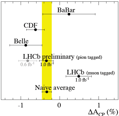
So far there is no evidence for CP-violation in measurements of the CP asymmetries induced by the interference between mixing and decay amplitudes. However, the firsts LHCb measurements of the direct CP asymmetries in $D\rightarrow\pi^{+}\pi^{-}$ and $D\rightarrow K^{+}K^{-}$ decays indicated a somewhat surprising large effect. The LHCb measurement of $\Delta A_{CP}=A_{CP}(K^{+}K^{-})-A_{CP}(\pi^{+}\pi^{-})$ using self-tagged $D^{*\pm}\rightarrow D^{0}[h^{+}h^{-}]\pi^{\pm}$ decays indicated some evidence for a non-zero CP asymmetry: $\Delta A_{CP}=(-0.82\pm 0.24)\%$ [37]. Later both CDF ($\Delta A_{CP}=(-0.62\pm 0.23)\%$ [38]) and Belle ($\Delta A_{CP}=(-0.87\pm 0.41)\%$ [39]) confirmed this measurement and increased the hopes that NP could be finally seen at work.

The measurement of $\Delta A_{CP}$ is protected from large systematic uncertainties as to first order detector and production asymmetries cancel in the subtraction. Moreover, within the SM and the majority of NP models, there is no loss of sensitivity in the subtraction as the CP-asymmetry is expected to have opposite sign for $D\rightarrow K^{+}K^{-}$ and $D\rightarrow\pi^{+}\pi^{-}$. Within the SM, the use of U-spin and QCD-factorization hypotheses leads to a prediction for $\Delta A_{CP}$ of about four times the ratio between the penguin amplitude (suppressed by $\lambda^{5}$) and the tree amplitude (only suppressed by $\lambda$), therefore the natural SM expectation is below $0.1\%$ [40, 41]. NP effects could enlarge this asymmetry to the level seen experimentally, however the SM prediction also has sizable uncertainties (see e.g. Ref. [42, 43, 44, 45]). In particular, the U-spin approximation is already challenged by the fact that the branching ratio of $D\rightarrow\pi^{+}\pi^{-}$ is measured to be different (about three times larger) than the branching ratio of $D\rightarrow K^{+}K^{-}$. This fact could be the hint of large non-perturbative effects enhancing also the SM prediction of $\Delta A_{CP}$ [46]. As described in Ref. [47], a valuable tool to distinguish SM vs. NP contributions to $\Delta A_{CP}$ is provided, in principle, by the analysis of direct CP asymmetries in radiative modes ($D\rightarrow K^{+}K^{-}\gamma$ and $D\rightarrow\pi^{+}\pi^{-}\gamma$).

Recently, LHCb has updated the measurement including up to one third of the data already on tape. The new measurement, $\Delta A_{CP}=(-0.34\pm 0.18)\%$ [48], does not confirm the initial indications. Moreover, LHCb has performed a complementary analysis using self-tagged $B^{\pm}\rightarrow D^{0}[h^{+}h^{-}]\mu^{\pm}\nu X$ events and measured $\Delta A_{CP}=(0.49\pm 0.33)\%$ [49]. The naive world average gives $\Delta A_{CP}=(-0.33\pm 0.12)\%$ with an internal consistency that has a probability of $3.7\%$ to occur. The consistency of these measurements is ilustrated in Fig.4. The results from LHCb are completely dominated by the statistical uncertainty and therefore the situation will become more clear in the near future when the 3/fb^-1 of data already on tape are analyzed.

The family of EW penguins involves only quarks, leptons and weak bosons to first order therefore the uncertainty due to QCD corrections is reduced compared with the dominant pure QCD penguins where the weak bosons are replaced by gluons. An example of its simplest realization can be seen in the left panel of Fig. 5 and consist on a photon emited from the internal loop. If the photon decays into a lepton pair (hence the amplitude is further suppressed by a factor $\alpha_{\rm{QED}}$) or it is replaced by a Z boson, the process can provide a rich laboratory to test NP models. An example is shown on the center panel on Fig. 5.

The inclusive process $b\rightarrow s\gamma$ has been measured precisely at the B-factories, CESR and LEP with an uncertainty of $\sim 7\%$, $BR(b\rightarrow s\gamma)=(3.55\pm 0.26)\times 10^{-4}$ [71], in agreement with the SM prediction, $BR(b\rightarrow s\gamma)=(3.15\pm 0.23)\times 10^{-4}$ [51]. In fact, this measurement is one of the strongest constraints in supersymmetric extensions of the SM. Inclusive measurements are difficult at hadron colliders, but exclusive radiative decays are measured at LHCb with high statistics, (5300/fb^-1 $B\rightarrow K^{*}\gamma$ and 700/fb^-1 $B_{s}\rightarrow\phi\gamma$ candidates). LHCb has already provided the most precise measurement of the radiative $B_{s}$ branching ratio: $BR(B_{s}\rightarrow\phi\gamma)=(3.5\pm 0.4)\times 10^{-5}$ [52], however the theory predictions for these exclusive decays are not precise enough. In the near future, precise measurements of the photon polarization in these decays could be a promising search for NP effects.

The decay $B\rightarrow K^{*}\mu^{+}\mu^{-}$ is the ”golden mode” to test new vector(axial-vector) couplings contributing to the loops in $b\rightarrow s$ transitions, complementing the sensitivity to NP operators in radiative decays. The sign of the pion in the decay $K^{*}\rightarrow K^{\pm}\pi^{\mp}$ allows to tag the flavour of the $B$-meson, hence an angular analysis can be unambigously performed to test the helicity structure of the EW penguin. If we define $\theta_{l}$, as the polar angle of the negative lepton and the direction opposite that of the $\bar{B_{d}}$ in the dimuon rest frame, $\theta_{K}$ the angle of the negative kaon in the $\bar{K^{*}}$ rest frame and $\phi$ the angle between the two planes defined by ($K,\pi$) and ($\mu^{+},\mu^{-}$) in the $\bar{B_{d}}$ rest frame, we can write the differential branching ratio as a function of these angles and $q^{2}$ with only four parameters: $F_{L},S_{3},A_{FB}$ and $A_{IM}$. Hadronic uncertainties in the predictions for these parameters are under reasonable control. $F_{L}$ indicates the fraction of longitudinal polarization in $K^{*}$ and $A_{FB}$ measures the forward-backward asymmetry of the lepton. Both parameters are expected to have a strong dependence on $q^{2}$. $S_{3}$ measures the asymmetry in the $K^{*}$ transverse polarization and $A_{IM}$ is proportional to the T-odd CP asymmetry. These last two parameters are expected to be very small and mostly independent of $q^{2}$ given the current level of precision. The first angular analyses of the decay $B\rightarrow K^{*}\mu^{+}\mu^{-}$ performed at the BaBar, Belle and CDF experiments were limited by the large statistical uncertainties [53, 54, 55]. Recently, the LHC experiments have taken over. The LHCb experiment [60] with only 1 fb^-1 has the largest sample of $B\rightarrow K^{*}\mu^{+}\mu^{-}$ candidates (900/fb^-1) with very small background and therefore has the best sensitivity, but also ATLAS [56] and CMS [57] with $\sim$80/fb^-1 candidates are competitive, in particular at large values of $q^{2}$. In Fig. 6 the measurements of the parameter $A_{FB}$ by the LHC experiments are compared with previous measurements and the SM predictions. The precision achieved by the LHCb experiment allows for a determination of the zero crossing-point for the first time: $q^{2}(A_{FB}=0)=4.9\pm 0.9~\rm{GeV}^{2}$ which is in good agreement with the relatively more precise SM prediction: $4.4\pm 0.3~\rm{GeV}^{2}$ [61].¹¹ 1  Kinematical studies of $B\rightarrow K^{*}\mu^{+}\mu^{-}$ at LHCb have significantly improved after the completion of this review, that reflects the status of flavor-physics observables before the summer 2013. In particular, a significant discrepancy between SM predictions and the so-called $P_{5}^{\prime}$ asymmetry [63] in the low-$q^{2}$ region has recently been observed at LHCb [62]. This result has triggered a significant amount of theoretical/phenomenological work, mainly focused on a reliable re-analysis of the (SM) theoretical error on $P_{5}$ [64, 65, 67, 68, 66], that is likely to be underestimated (see also Ref. [69]). We refer to these recent papers for a more detailed discussion about this point.

There are other observables and many other decay modes sensitive to NP affecting the EW penguin which are being studied or will be available with more statistics. The increase in precision of these analyses will allow for one of the strongest tests of generic NP models, up to some level independent of the NP flavour structure.

The pure leptonic decays of $K,D$ and $B$-mesons are a particularly interesting case of EW penguins, see right panel of Fig. 5. Compared with the decays described in section 4.3, the helicity configuration of the final state suppresses the vector(axial-vector) contribution by a factor proportional to $({m_{l}}/{M_{K,D,B}})^{2}$. Therefore, these decays are particularly sensitive to new (pseudo-)scalar interactions. This is why they are sometimes referred as ”Higgs-penguins” [70].

In the case of $K$ and $D$-meson decays, the contribution of the absorptive part in the amplitude can be dominant. Indeed, this is what is observed in the measurement of $BR(K_{L}\rightarrow\mu^{+}\mu^{-})=(6.84\pm 0.11)\times 10^{-9}$ [71]. The equivalent contribution to the $K_{s}$ decay is calculated to be $\sim 5\times 10^{-12}$ [72, 73], therefore if $BR(K_{s}\rightarrow\mu^{+}\mu^{-})$ is measured to be larger than $10^{-11}$ it should be a clear indication of NP in the dispersive contribution, and should certainly increase the interest in measurements like the $BR(K^{+}\rightarrow\pi^{+}\nu\nu)$. The excellent invariant mass resolution of the LHCb experiment, together with the large production of kaons at the LHC ($10^{13}K_{s}$/fb^-1) has allowed LHCb to improve drastically (by a factor 30) the limit on $BR(K_{s}\rightarrow\mu^{+}\mu^{-})$. With 1 fb^-1 of data LHCb obtains a limit of $BR(K_{s}\rightarrow\mu^{+}\mu^{-})<9\times 10^{-9}$ at $90\%$CL [74], similar to the limit obtained by KLOE on $BR(K_{s}\rightarrow e^{+}e^{-})<9\times 10^{-9}$ at $90\%$CL [75].

In the case of D-meson decays the absorptive contribution is limited by the measured $BR(D\rightarrow\gamma\gamma)$ at BABAR [76] to be up to $6\times 10^{-11}$ [77]. Again the excellent LHCb detector performance and large charm production at the LHC has allowed to improve the existing results (by a factor 20), $BR(D\rightarrow\mu^{+}\mu^{-})<6.2\times 10^{-9}$ at $90\%$CL [78]. Although these are certainly large improvements, the LHCb results have been obtained with only one third of the data already available. The experiment expects to collect the equivalent of two orders of magnitude more data in the next decade (taking into account the increase in cross-section at higher energies). Therefore, we should expect that the interesting region between $10^{-11}$ and $10^{-9}$ is explored in the next decade for $K$- and $D$-mesons decays.

In the case of $B_{d}$ and $B_{s}$-meson decays the contribution of the absorptive part can be safely neglected. These decays are well predicted theoretically and experimentally are exceptionally clean, in particular the $B_{s}$ decay. Using tree level measurements as described in Sect. 3, the SM predictions are [79, 80, 81] (see also  [82]): $BR(B_{s}\rightarrow\mu^{+}\mu^{-})=(3.65\pm 0.23)\times 10^{-9}$ and $BR(B_{s}\rightarrow\mu^{+}\mu^{-})=(1.06\pm 0.09)\times 10^{-10}$. In the $B_{s}$ case, this prediction corresponds to a flavour-averaged time-integrated measurement, taking into account the correction due to the non-vanishing width difference between $B_{s}$ and $\bar{B}_{s}$ mesons [83]. As mentioned before, these decays are superb tests for new (pseudo-)scalar contributions. In particular, within the Minimal Supersymmetric Standard Model the purely leptonic $B$-meson branching ratios are proportional to $\tan^{6}\beta/M^{4}_{A}$, where $\tan\beta$ denotes the ratio of the two Higgs vacuum expectation values, and $M_{A}$ the mass of the pseudo-scalar Higgs. Therefore these decays are very sensitive probes of the large ”$\tan\beta$” regime (see Sect. 5 for more details).

The main difficulty of the experimental analysis is the very large ratio between the background and the expected signal. For instance, if we assume the SM value branching ratio after the trigger and selection procedures, CDF [84] expects $\sim 0.26~B_{s}\rightarrow\mu^{+}\mu^{-}$ candidates per fb^-1, ATLAS [86] $\sim 0.4$, CMS [87] $\sim 0.8$ and LHCb [88] $\sim 3.6$ (with the multivariate discriminant (BDT)$>$0.7). The background (in the $B_{s}$ mass window) is dominated by combinations of real muons and it is estimated from the mass sidebands. Therefore the main handle to reduce the combinatorial background is the invariant mass resolution of the experiments, where a factor two better resolution is equivalent to a factor two more luminosity: ATLAS 80 MeV/$\rm{c}^{2}$, CMS 45 MeV/$\rm{c}^{2}$, CDF 25 MeV/$\rm{c}^{2}$ and LHCb 22 MeV/$\rm{c}^{2}$. Taking into account the previous estimates 1 fb^-1 at LHCb is roughly equivalent to 10 fb^-1 at CMS and 20 fb^-1 at ATLAS/CDF for the same analysis strategies. LHCb is also using the shape of the signal probability in invariant mass and multivariate discriminant distributions from control channels ($B_{d}\rightarrow h^{+}h^{{}^{\prime}-}$), rather than doing a simple counting experiment.

The results of the search for the decay $B_{s}\rightarrow\mu^{+}\mu^{-}$ from the Tevatron [84, 85] and LHC [86, 87, 88] experiments is summarized at the left panel of Fig. 7. CDF observes a slight excess with respect to the background only hypothesis with a probability of $\sim 0.9\%$ while the LHCb sensitivity allows to quote a first evidence for this decay with the probability of being a background fluctuation of $\sim 0.0005\%$ (equivalent to $3.5\sigma$). LHCb determines $BR(B_{s}\rightarrow\mu^{+}\mu^{-})=(3.2^{+1.5}_{-1.2})\times 10^{-9}$ in excellent agreement with the SM expectation. The invariant mass distribution obtained by LHCb can be seen at the right panel in Fig. 7. The search for the decay $B_{d}\rightarrow\mu^{+}\mu^{-}$ does not show a significant excess with respect to the background only hypothesis, and the best limit is obtained by LHCb to be: $BR(B_{d}\rightarrow\mu^{+}\mu^{-})<9.4\times 10^{-10}$ at $95\%$CL.

Very recently the CMS and LHCb Collaborations have updated their results for the summer 2013 conferences including the full datasets ($\sim 25$ fb^-1 from CMS and $\sim 3$ fb^-1 from LHCb). Both collaborations see clear evidence for the decay $B_{s}\rightarrow\mu^{+}\mu^{-}$ with significances larger or equal to $4\sigma$ for each individual measurement. The CMS measurement [89], $BR(B_{s}\rightarrow\mu^{+}\mu^{-})=(3.0^{+1.0}_{-0.9})\times 10^{-9}$ and the LHCb measurement [90], $BR(B_{s}\rightarrow\mu^{+}\mu^{-})=(2.9^{+1.1}_{-1.0})\times 10^{-9}$ are compatible and also in agreement with the SM. A preliminary combination of these two measurements gives [91], $BR(B_{s}\rightarrow\mu^{+}\mu^{-})=(2.9\pm 0.7)\times 10^{-9}$ which corresponds to a clear observation of this decay in agreement with the SM expectation. In the case of the $B_{d}$ decays, both collaborations do not claim yet a significant excess and quote a limit, $BR(B_{d}\rightarrow\mu^{+}\mu^{-})<1.1\times 10^{-9}$ at $95\%$CL from CMS and $BR(B_{d}\rightarrow\mu^{+}\mu^{-})<7.4\times 10^{-10}$ at $95\%$CL from LHCb.

If physics beyond the SM respects the SM gauge symmetry, as we expect from general arguments, the low-energy amplitudes describing the transition of a fermion $\psi_{i}$ to a fermion $\psi_{j}$ (of different flavour) can be decomposed in the following general form

where $\Lambda$ is the energy scale of the new degrees of freedom and the SM result is recovered in the limit $c_{\rm NP}\to 0$. This structure is completely general: the coefficients $c_{\rm SM(NP)}$ may include appropriate CKM coefficient factors and eventually a $\sim 1/(16\pi^{2})$ suppression if the amplitude is loop-mediated. Given our ignorance about the $c_{\rm NP}$ coefficients, the values of the scale $\Lambda$ probed by present experiments vary over a wide range. However, the general result in Eq. (22) allows us to predict how these bounds will improve with future experiments: increasing the statistic on a given observable, the corresponding bound on $\Lambda$ scales at most as $N^{1/4}$, where $N$ is the relative increase in the number of events used to measure the observable.²² 2 Let’s consider separately forbidden SM processes ($c_{\rm NP}\gg c_{\rm SM}$) and processes where NP is expected to be a small correction over the SM ($c_{\rm NP}\ll c_{\rm SM}$). In the first case, assuming negligible background, the experimental bound on the forbidden rate scales linearly with $N$ and the predicted rate of the process scales as $1/\Lambda^{4}$. In the second case, assuming a positive signal has already been observed, the improvement on the experimental precision scales as $N^{-1/2}$ and the bound is set on the interference term between SM and NP, that scales as $1/\Lambda^{2}$. As a result, in both cases the sensitivity on $\Lambda$ scales as $N^{1/4}$. From Eq. (22) it is also clear that indirect searches can probe NP scales well above the TeV for models where ($c_{\rm SM}\ll c_{\rm NP}$), namely models which do not respect the symmetries and the symmetry-breaking pattern of the SM.

As discussed in the previous section, the main strategy to search (or to constrain) physics beyond the SM in flavour-violating observables consists of two steps: i) determine the CKM elements from processes that are tree-level dominated within the SM (such that ${c_{\rm SM}}\gg{c_{\rm NP}}$), ii) use these values to predict loop-mediated amplitudes and compare them with the corresponding measurements, allowing for non-vanishing NP effects. An illustration of this procedure in the case of the two $B_{d,s}$-meson mixing amplitudes is shown in Fig. 8 [92]. The possible NP contributions to $B_{s,d}$-meson mixing are parameterized in terms of two complex parameters, $\Delta_{s,d}$, describing the normalization of the amplitude with respect to the SM case (the SM is recovered for $\Delta_{s}=\Delta_{d}=1$). The results of the fit to data allowing for generic $\Delta_{s,d}$, is reported in Fig. 8. As can be seen, the present data are in good agreement with the SM expectation. On the other hand, non-vanishing NP contributions of $O(20\%)$ for both $|\Delta_{s}|$ and $|\Delta_{d}|$, and up to $0.1$ and $0.05$ for $\phi_{s}={\rm arg}(\Delta_{s})$ and $\phi_{d}={\rm arg}(\Delta_{d})$, respectively, are still allowed.

Assuming NP is heavy, the experimental bounds on the effective couplings $\Delta_{s,d}$ can be translated into bounds on the couplings of effective NP local operators (generated by the exchange of the heavy new states) contributing to the $B_{s,d}$-meson mixing amplitudes. In Table 1 we report such bounds for the most representative $\Delta F=2$ operators (i.e. operators contributing to meson-antimeson mixing at the tree level), together with similar bounds obtained from meson-antimeson mixing in the kaon and $D$-meson systems.³³ 3 For the definition of the observables describing CP violation in the neutral kaon system ($\epsilon_{K}$ and $\epsilon^{\prime}$) and those describing CP violation in the $D$-meson mixing amplitude ($|q/p|_{D}$ and $\phi_{D}$) we refer to Ref. [93] and [94], respectively. Updated constraints on $D$-meson mixing parameters can be found in Ref. [95]. As can be seen, for $c_{\rm NP}=1$ present data probes very high scales. On the other hand, if we insist with the theoretical prejudice that NP must show up not far from the TeV scale in order to stabilize the Higgs sector, then the new degrees of freedom must have a peculiar flavour structure able to justify the smallness of the effective couplings $c_{\rm NP}$ for $\Lambda=1$ TeV (this fact is often known as the NP flavour problem).

A natural suppression of the $c_{\rm NP}$ is obtained under the so-called hypothesis of Minimal Flavour Violation (MFV) [99, 98, 100]. The main idea of MFV is that flavour-violating interactions are linked to the known structure of Yukawa couplings also beyond the SM. In a more quantitative way, the MFV construction consists in identifying the flavour symmetry and symmetry-breaking structure of the SM and enforce it also beyond the SM.

The MFV hypothesis consists of two ingredients: (i) a flavour symmetry and (ii) a set of symmetry-breaking terms [100]. The symmetry is nothing but the large global symmetry ${\mathcal{G}}_{\rm flavour}$ of the SM Lagrangian in absence of Yukawa couplings shown in Eq. (4). Since this global symmetry, and particularly the ${SU}(3)$ subgroups controlling quark flavour-changing transitions, is already broken within the SM, we cannot promote it to be an exact symmetry of the NP model. Some breaking would appear at the quantum level because of the SM Yukawa interactions. The most restrictive assumption we can make to protect in a consistent way quark-flavour mixing beyond the SM is to assume that $Y_{d}$ and $Y_{u}$ are the only sources of flavour symmetry breaking also in the NP model. If the breaking of the symmetry occurs at very high energy scales, at low-energies we would only be sensitive to the background values of the $Y$, i.e. to the ordinary SM Yukawa couplings. The role of the Yukawa in breaking the flavour symmetry becomes similar to the role of the Higgs in the breaking of the gauge symmetry. However, in the case of the Yukawa we don’t know (and we do not attempt to construct) a dynamical model which gives rise to this symmetry breaking.

Within a generic effective-theory approach to physics beyond the SM, we can say that an effective theory satisfies the MFV criterion if all higher-dimensional operators, constructed from SM and $Y_{d,u}$ spurion fields, are invariant under CP and (formally) under the flavour group ${\mathcal{G}}_{q}$ [100]. According to this criterion one should in principle consider operators with arbitrary powers of the (dimensionless) Yukawa fields. However, a strong simplification arises by the observation that all the eigenvalues of the Yukawa matrices are small, but for the one corresponding to the top quark, and that the off-diagonal elements of the CKM matrix are very suppressed. Working in the basis in Eq. (6) we have

As a consequence, in the limit where we neglect light quark masses, the leading $\Delta F=2$ and $\Delta F=1$ FCNC amplitudes get exactly the same CKM suppression as in the SM:

where the $\mathcal{A}^{(i)}_{\rm SM}$ are the SM loop amplitudes and the $a_{i}$ are $O(1)$ real parameters. The $a_{i}$ depend on the specific operator considered but are flavour independent. This implies the same relative correction in $s\to d$, $b\to d$, and $b\to s$ transitions of the same type: a key prediction which can be tested in experiment.

References

- (1) G. Aad et al. [ATLAS Collaboration], Phys. Lett. B 716 (2012) 1
- (2) S. Chatrchyan et al. [CMS Collaboration], Phys. Lett. B 716 (2012) 30
- (3) N. Cabibbo, Phys. Rev. Lett. 10 (1963) 531.
- (4) M. Kobayashi and T. Maskawa, Prog. Theor. Phys. 49 (1973) 652.
- (5) A. J. Buras and J. Girrbach, arXiv:1306.3775.
- (6) L. -L. Chau and W. -Y. Keung, Phys. Rev. Lett. 53 (1984) 1802.
- (7) L. Wolfenstein, Phys. Rev. Lett. 51 (1983) 1945.
- (8) Y. Amhis et al. [HFAG Collaboration], arXiv:1207.1158.
- (9) K. Hara et al. [Belle Collaboration], Phys. Rev. Lett. 110 (2013) 131801.
- (10)
J. Charles et al. [CKMfitter group],
Eur. Phys. J. C 41 (2005) 1,
updated results available at: http://ckmfitter.in2p3.fr - (11)
M. Bona et al. [UTfit Collaboration],
JHEP 0610 (2006) 081,
updated results available at: http://www.utfit.org - (12) J. P. Lees et al [BABAR Collaboration], Phys. Rev. Lett. 109 (2012) 101802.
- (13) M. Gronau and D. London, Phys. Lett. B 253 (1991) 483.
- (14) M. Gronau and D. Wyler, Phys. Lett. B 265 (1991) 172.
- (15) D. Atwood, I. Dunietz and A. Soni, Phys. Rev. Lett. 78 (1997) 3257.
- (16) A. Giri, Y.Grossman, A. Soffer and J. Zupan, Phys. Rev. D 68 (2003) 054018.
- (17) P. del Amo Sanchez et al. [BABAR Collaboration], Phys. Rev. D 82 (2010) 072004.
- (18)
J. P. Lees et al. [BABAR Collaboration], Phys. Rev. D 84 (2011) 012002,
and the combination of BABAR results as shown at: http:www.physics.uc.eduschwartzCKM2012. - (19) A. Poluektov et al. [Belle Collaboration], Phys. Rev. D 81 (2010) 112002.
- (20) Y. Horii et al. [Belle Collaboration], Phys. Rev. Lett. 106 (2011) 231803.
- (21)
H. Aihara et al. [Belle Collaboration], Phys. Rev. D 85 (2012) 112014,
and the combination of Belle results as shown at: http:www.physics.uc.eduschwartzCKM2012. - (22) R. Aaij et al. [LHCb Collaboration], Phys. Lett. B 712 (2012) 203.
- (23) R. Aaij et al. [LHCb Collaboration], LHCb-CONF-2013-004.
- (24) R. Aaij et al. [LHCb Collaboration], LHCb-CONF-2013-006.
- (25) R. Aaij et al. [LHCb Collaboration], New J. Phys. 15 (2013) 053021.
- (26) B. Aubert et al. [BABAR Collaboration], Phys. Rev. D 79 (2009) 072009.
- (27) I. Adachi et al. [Belle Collaboration], Phys. Rev. Lett. 108 (2012) 171802.
- (28) R. Aaij et al. [LHCb Collaboration], Phys. Rev. Lett. 108 (2012) 101803.
- (29) R. Aaij et al. [LHCb Collaboration], Phys. Rev. D 87 (2013) 112010.
- (30) A. Lenz and U. Nierste, arXiv:1102.4274.
- (31) V.M. Abazov et al. [D0 Collaboration], Phys. Rev. D 84 (2011) 052007.
- (32) K. Abe et al. [Belle Collaboration], Phys. Rev. D 73 (2006) 112002.
- (33) B. Aubert et al. [BABAR Collaboration], Phys. Rev. Lett. 96 (2006) 251802.
- (34) V.M. Abazov et al. [D0 Collaboration], Phys. Rev. D 86 (2012) 072009.
- (35) V.M. Abazov et al. [D0 Collaboration], Phys. Rev. Lett. 110 (2013) 011801.
- (36) R. Aaij et al. [LHCb Collaboration], LHCb-CONF-2012-022.
- (37) R. Aaij et al. [LHCb Collaboration], Phys. Rev. Lett. 108 (2012) 111602.
- (38) T. Aaltonen et al. [CDF Collaboration], Phys. Rev. Lett. 109 (2012) 111801.
- (39) B.R. Ko et al. [Belle Collaboration], Proceedings of ICHEP 2012 (2013).
- (40) Y. Grossman, A. L. Kagan and Y. Nir, Phys. Rev. D 75 (2007) 036008.
- (41) G. Isidori, J. F. Kamenik, Z. Ligeti and G. Perez, Phys. Lett. B 711 (2012) 46.
- (42) M. Golden and B. Grinstein, Phys. Lett. B 222 (1989) 501.
- (43) J. Brod, A. L. Kagan and J. Zupan, Phys. Rev. D 86 (2012) 014023.
- (44) D. Pirtskhalava and P. Uttayarat, Phys. Lett. B 712 (2012) 81.
- (45) E. Franco, S. Mishima and L. Silvestrini, JHEP 1205 (2012) 140.
- (46) J. Brod, Y. Grossman, A. L. Kagan and J. Zupan, JHEP 1210 (2012) 161.
- (47) G. Isidori and J. F. Kamenik, Phys. Rev. Lett. 109 (2012) 171801.
- (48) R. Aaij et al. [LHCb Collaboration], LHCb-CONF-2013-003.
- (49) R. Aaij et al. [LHCb Collaboration], Phys. Lett. B 723 (2013) 33.
- (50) B. Aubert et al. [BABAR Collaboration], Phys. Rev. Lett. 100 (2008) 061803.
- (51) M. Misiak et al., Phys. Rev. Lett. 98 (2007) 022002.
- (52) R. Aaij et al. [LHCb Collaboration], Nucl. Phys. B 867 (2013) 1.
- (53) B. Aubert et al. [BABAR Collaboration], Phys. Rev. D 73 (2006) 092001.
- (54) J.-T. Wei et al. [Belle Collaboration], Phys. Rev. Lett. 103 (2009) 171801.
- (55) T. Aaltonen et al. [CDF Collaboration], Phys. Rev. Lett. 108 (2012) 081807.
- (56) G. Aad et al. [ATLAS Collaboration], ATLAS-CONF-2013-038.
- (57) S. Chatrchyan et al. [CMS Collaboration], ,” Phys. Lett. B 727 (2013) 77.
- (58) C. Bobeth, G. Hiller and D. van Dyk, JHEP 1107 (2011) 067.
- (59) C. Bobeth, G. Hiller and D. van Dyk, Phys. Rev. D 87, 034016 (2013).
- (60) R. Aaij et al. [LHCb Collaboration], JHEP 1308 (2013) 131.
- (61) M. Beneke, T. Feldmann and D. Seidel, Eur. Phys. J. C 41 (2005) 173.
- (62) RAaij et al. [LHCb Collaboration], Phys. Rev. Lett. 111 (2013) 191801.
- (63) S. Descotes-Genon, T. Hurth, J. Matias and J. Virto, JHEP 1305 (2013) 137.
- (64) W. Altmannshofer and D. M. Straub, Eur. Phys. J. C 73 (2013) 2646.
- (65) C. Hambrock, G. Hiller, S. Schacht and R. Zwicky, arXiv:1308.4379.
- (66) F. Beaujean, C. Bobeth and D. van Dyk, arXiv:1310.2478.
- (67) S. Descotes-Genon, J. Matias and J. Virto, Phys. Rev. D 88 (2013) 074002, and arXiv:1311.3876.
- (68) T. Hurth and F. Mahmoudi, JHEP 1404 (2014) 097.
- (69) S. Jger and J. Martin Camalich, JHEP 1305 (2013) 043.
- (70) A. Dedes, Mod. Phys. Lett. A 18 (2003) 2627.
- (71) J. Beringer et al. [Particle Data Group], Phys. Rev. D 86 (2012) 010001.
- (72) G. Ecker and A. Pich, Nucl. Phys. B 366 (1991) 189.
- (73) G. Isidori and R. Unterdorfer, JHEP 0401 (2004) 009.
- (74) R. Aaij et al. [LHCb Collaboration], JHEP 1301 (2013) 090.
- (75) F. Ambrosino et al. (KLOE Collaboration], Phys. Lett. B 672 (2009) 203.
- (76) J. P. Lees et al. [BABAR Collaboration], Phys. Rev. D 85 (2012) 091107.
- (77) G. Burdman, E. Golowich, J.L. Hewett and S. Pakvasa, Phys. Rev. D 66 (2002) 014009.
- (78) RAaij et al. [LHCb Collaboration], Phys. Lett. B 725 (2013) 15.
- (79) C. Bobeth, M. Gorbahn, T. Hermann, M. Misiak, E. Stamou and M. Steinhauser, Phys. Rev. Lett. 112 (2014) 101801.
- (80) T. Hermann, M. Misiak and M. Steinhauser, JHEP 1312 (2013) 097.
- (81) C. Bobeth, M. Gorbahn and E. Stamou, Phys. Rev. D 89 (2014) 034023.
- (82) A. J. Buras, J. Girrbach, D. Guadagnoli and G. Isidori, Eur. Phys. J. C 72 (2012) 2172.
- (83) K. de Bruyn et al., Phys. Rev. Lett. 109 (2012) 041801.
- (84) T. Aaltonen et al. [CDF Collaboration], Phys. Rev. Lett. 107 (2011) 191801.
- (85) V. M. Abazov et al. [D0 Collaboration], Phys. Lett. B 693 (2010) 539.
- (86) G. Aad et al. [ATLAS Collaboration], Phys. Lett. B 713 (2012) 387.
- (87) S. Chatrchyan et al. [CMS Collaboration], JHEP 1204 (2012) 033.
- (88) R. Aaij et al. [LHCb Collaboration], Phys. Rev. Lett. (110) 021801 (2013).
- (89) Phys. Rev. Lett. 111 (2013) 101804.
- (90) RAaij et al. [LHCb Collaboration], Phys. Rev. Lett. 111 (2013) 101805.
- (91) The CMS and LHCb Collaborations, CMS-PAS-BPH-13-007, LHCb-CONF-2013-012.
- (92) A. Lenz et al., Phys. Rev. D 86 (2012) 033008.
- (93) G. D’Ambrosio and G. Isidori, Int. J. Mod. Phys. A 13 (1998) 1.
- (94) O. Gedalia, Y. Grossman, Y. Nir and G. Perez, Phys. Rev. D 80 (2009) 055024.
- (95) A. J. Bevan et al. [UTfit Collaboration], JHEP 1210 (2012) 068.
- (96) G. Isidori, Y. Nir and G. Perez, Ann. Rev. Nucl. Part. Sci. 60 (2010) 355.
- (97) G. Isidori, arXiv:1302.0661.
- (98) L. J. Hall and L. Randall, Phys. Rev. Lett. 65 (1990) 2939.
- (99) R. S. Chivukula and H. Georgi, Phys. Lett. B 188 (1987) 99.
- (100) G. D’Ambrosio, G. F. Giudice, G. Isidori and A. Strumia, Nucl. Phys. B 645 (2002) 155.
- (101) A. J. Buras, P. Gambino, M. Gorbahn, S. Jager and L. Silvestrini, Phys. Lett. B 500 (2001) 161.
- (102) D. Guadagnoli and G. Isidori, Phys. Lett. B 724 (2013) 63.
- (103) A. L. Kagan, G. Perez, T. Volansky and J. Zupan, Phys. Rev. D 80 (2009) 076002.
- (104) O. Buchmueller et al., Eur. Phys. J. C 72 (2012) 2243.
- (105) O. Buchmueller et al., Eur. Phys. J. C 72 (2012) 1878.
- (106) F. Mahmoudi, arXiv:1205.3099.
- (107) R. Barbieri, G. Isidori, J. Jones-Perez, P. Lodone and D. M. Straub, Eur. Phys. J. C 71 (2011) 1725.
- (108) R. Barbieri, D. Buttazzo, F. Sala and D. M. Straub, JHEP 1207 (2012) 181.
- (109) M. Papucci, J. T. Ruderman and A. Weiler, JHEP 1209 (2012) 035.
- (110) J. R. Espinosa, C. Grojean, V. Sanz and M. Trott, JHEP 1212 (2012) 077.
- (111) A. Delgado, G. F. Giudice, G. Isidori, M. Pierini and A. Strumia, Eur. Phys. J. C 73 (2013) 2370.
- (112) D. B. Kaplan, Nucl. Phys. B 365 (1991) 259.
- (113) K. Agashe, G. Perez and A. Soni, Phys. Rev. D 71 (2005) 016002.
- (114) S. Davidson, G. Isidori and S. Uhlig, Phys. Lett. B 663 (2008) 73.
- (115) B. Keren-Zur et al., Nucl. Phys. B 867 (2013) 429.
- (116) M. Redi and A. Weiler, JHEP 1111 (2011) 108.
- (117) R. Barbieri, D. Buttazzo, F. Sala and D. M. Straub, JHEP 1210 (2012) 040.
- (118) R. Barbieri, D. Buttazzo, F. Sala, D. M. Straub and A. Tesi, JHEP 1305 (2013) 069.
- (119) Y. Nomura, M. Papucci and D. Stolarski, Phys. Rev. D 77 (2008) 075006.
- (120) NA62 Collaboration: Technical Design Document/ NA62-10-07 (2010), https:cdsweb.cern.chrecord1404985.