Optimization of random search processes in the presence of an external bias
Abstract
We study the efficiency of random search processes based on Lévy flights with power-law distributed jump lengths in the presence of an external drift, for instance, an underwater current, an airflow, or simply the bias of the searcher based on prior experience. While Lévy flights turn out to be efficient search processes when relative to the starting point the target is upstream, in the downstream scenario regular Brownian motion turns out to be advantageous. This is caused by the occurrence of leapovers of Lévy flights, due to which Lévy flights typically overshoot a point or small interval. Extending our recent work on biased LF search [V. V. Palyulin, A. V. Chechkin, and R. Metzler, Proc. Natl. Acad. Sci. USA, 111, 2931 (2014).] we establish criteria when the combination of the external stream and the initial distance between the starting point and the target favors Lévy flights over regular Brownian search. Contrary to the common belief that Lévy flights with a Lévy index (i.e., Cauchy flights) are optimal for sparse targets, we find that the optimal value for may range in the entire interval and include Brownian motion as the overall most efficient search strategy.
pacs
05.40.-a,05.40.Jc,05.10.GgI Introduction
To find a lost key on a parking lot or a paper on an untidy desk are typical everyday experiences for search problems [1, 2]. Search processes occur on many different scales, ranging from the passive diffusive search of regulatory proteins for their specific binding site in living biological cells [3] over the search of animals for food [4, 5] or of computer algorithms for minima in a complex search space [6]. Here we are interested in random, jump-like search processes. The searcher, that is, has no prior information on the location of its target and performs a random walk until encounter with the target. During a relocation along its trajectory (a jump), the walker is insensitive to the target. In the words of movement ecology occupied with the movement patterns of animals, this process is called blind search with saltatory motion. It is typical for predators hunting at spatial scales exceeding their sensory range [7, 8, 9, 10]. For instance, blind search is observed for plankton-feeding basking sharks [11], jellyfish predators and leatherback turtles [12], and southern elephant seals [13]. Saltatory search is distinguished from cruise search, when the searcher continues to explore its environment during relocations.
The first studies on random search considered the Brownian motion of the searcher as a default strategy, until Shlesinger and Klafter proposed that Lévy flights (LFs) are much more efficient in the search for sufficiently sparse targets [14]. In a Markovian LF the individual displacement lengths of the walker are power-law distributed, , where due to the second moment of the jump lengths diverges, [15]. This lack of a length scale effects a fractal dimension of the trajectory [16, 17], such that local search is interspersed by long, decorrelating excursions. This strategy avoids oversampling, the frequent return to previously visited points in space of recurrent random walk processes, such as Brownian motion in one and two dimensions [5, 14, 18, 19]. The latter are indeed the relevant cases for land-based searchers. Even for airborne or marine searchers, the vertical span of their trajectories is usually much smaller than the horizontal span, rendering their motion almost fully two dimensional. The outstanding role of LFs for random search processes in one and two dimensions was formulated in the LF hypothesis: Superdiffusive motion governed by fat-tailed propagators optimize encounter rates under specific (but common) circumstances: hence some species must have evolved mechanisms that exploit these properties [5].
Starting with the report of LF-search by albatross birds [20, 18] there was a surge of discoveries of such scale-free search strategies, inter alia, for marine predators [21, 22], insects such as moths [23], land-based mammals such as deer and goats [24, 25], as well as microorganisms such as dinoflagellates [26]. In some cases these reports were debated. For instance, an additional investigation showed that spider monkeys indeed move deterministically [27] and mussels have multimodal rather than power-law relocations [28, 29]. Similarly, plant lice exhibit Lévy motion on the population level but not for the motion of individuals [30]. In particular, the disqualification of the LF statistics for albatrosses [31] became a strong argument against the LF hypothesis. However, there is strong evidence that for individual albatross birds LFs are indeed a real search pattern [32].
From extensive studies of human trajectories it was shown that LF motion patterns are indeed characteristic [33, 34], although in some cases correlations in the motion exist [35]. Similarly the paths of fishing boats follow LF statistics [36], although this observation has also been put in question [37]. Interesting findings were reported from robotics, where one of the important questions is how robots should search for hidden targets. From simulations it was concluded that the most successful robots performed motion consistent with LF foraging [38].
A number of other search strategies was proposed as an alternative to LFs. These include intermittent dynamics switching between local diffusive search and ballistic relocations [39], which may also be of power-law form [40]. Moreover, searchers may perform persistent random walks with finite tangential correlations [41]. However, while the difference in performance between models with a scale and LFs may be small, the central advantage of the LF strategy is its robustness: while other models work best when their parameters are optimized for specific environmental conditions such as the target density LFs remain close to optimal even when these conditions are altered [40]. LFs have thus been promoted as a preferred strategy when there is insufficient prior knowledge on the search space. In particular, for sufficiently sparse targets several analyses claim that the optimal value for the power-law exponent is [18, 40, 42, 43, 44, 45, 46].
Following the continuing debate over the validity of the LF hypothesis we here extend our recent study in Ref. [47] and scrutinize the LF hypothesis from a different angle. Namely, we analyze the performance of the LF search mechanism in the presence of an external bias. Such a bias could, for instance, correspond to an underwater current biasing the search motion of marine predators or search robots, or to an airflow driving birds of prey in a preferential direction. It could be a bias in an abstract landscape searched by a computed algorithm. Finally, it could also simply be the personal bias of the searcher based on some prior experience. Such biases are commonplace and their effect needs to be considered in models for random search processes. It turns out that an external bias may have profound consequences for the efficiency of LF search. Thus, even in the presence of a small bias LF search may fare worse than Brownian search. Depending on the initial separation between searcher and target and on whether from the perspective of the searcher the bias is directed towards or away from the target, we find that the optimal power-law exponent may range in the entire interval from one to 2, and explicitly include Brownian motion. Without prior knowledge, it may turn out that Brownian search is indeed the more efficient search method.
The paper is organized as follows. In Sec. II we set up our model in terms of the fractional Fokker-Planck equation. In Sec. III we explicitly calculate the first arrival density and the search efficiency in absence of a bias. In particular, we obtain the optimal search parameters as function of the initial distance between searcher and target. In Sec. IV we generalize these findings to the case when an external bias is present. We analyze the temporal decay of the first arrival density and introduce a generalized Péclet number. We draw our Conclusions in Sec. V. In the Appendix, we detail several calculations.
II A Model
II.1 Solution of the Fokker-Planck equation with the sink term


Imagine the process depicted in Fig. 1. A random walker moves by random jumps, whose lengths are chosen according to the power-law distribution with
| (1) |
where denotes the Fourier transform of . Its stretched Gaussian form in space defines a symmetric Lévy stable distribution, with the long-tailed asymptotic form for . Consequently the variance of diverges, , while fractional moments of order are finite [16, 15]. In addition to such Lévy stable jump lengths we consider an external drift. This bias is called uphill (or downhill) when the bias is directed against (along) the walker with respect to the original walker-target location.
A searcher finds the target when after a jump its position coincides with the location of the target. That is, the successful search corresponds to the first arrival at the target coordinate. This process will be substantially different from that of Brownian search, and consists of a tradeoff between two effects: (i) due to the scale-free jump length distribution (1) the above-mentioned oversampling is diminished, and less points are revisited multiply before eventual location of the target. (ii) Due to the existence of extremely long jumps the walker may severely overshoot the target, producing so-called leapovers (see Fig. 1). The length of these leapovers is distributed as , and is thus wider than the original jump length distribution (1) [48]. This property renders the first arrival of an LF different from the process of first passage, and the first arrival efficiency worsens with decreasing [49].
The basis for the mathematical description of the first arrival process of LFs is the fractional Fokker-Planck equation for the density to find the searcher at position at time in the presence of an external force field [15, 50]. Generalizing the approach of Ref. [49], to describe the first arrival of a searcher to point , we remove the searcher from the target location by a -sink with time dependent weight ,
| (2) |
Here, denotes the constant external bias, is the generalized diffusion coefficient [15], and is the density of first arrival [49], as shown below. The fractional derivative of Riesz-Weyl form is defined in terms of its Fourier transform, , where is the Fourier transform of [15]. Eq. (2) is completed with the initial condition of placing the searcher at . If is positive, the drift is directed towards positive , that is, the dynamic equation (2) describes the situation of Fig. 1.
By rescaling of variables (see App. A) we obtain the dimensionless analog of Eq. (2),
| (3) |
where and . The factor has the dimension of length and is chosen as the scaling factor of the LF jump length distribution, as detailed in App. A. In what follows we use the dimensionless variables throughout, but for simplicity we omit the overlines. Without loss of generality we assume that in the remainder of this work. Integration of Eq. (3) over the position produces the first arrival density
| (4) |
Thus, is indeed the negative time derivative of the survival probability .
In analogy to the bias-free case [49] it is straightforward to obtain the Fourier-Laplace transform of the distribution ,
| (5) |
Here we express the Laplace image of a function by explicit dependence on the Laplace variable . Integration of Eq. (5) over the Fourier variable yields
| (6) |
where is the solution of Eq. (2) without the sink term. As this expression necessarily equals zero, the first arrival density can be expressed through
| (7) |
where we use the abbreviation
| (8) |
Equation (7) without bias () was obtained in Ref. [49]. An important observation from Eq. (7) is that the first arrival density vanishes, , for any if only (for the proof see App. B and C). Thus LF search for a point-like target will never succeed for . This property reflects the transience of LFs with , where is the dimension of the embedding space [51].
II.2 Langevin equation simulations
For the simulation of LFs we use the Langevin equation approach, which in the discretized version with dimensionless units takes on the form [52]
| (9) |
where is the (dimensionless) position of the walker at the -th step, and is a set of random variables with Lévy stable distribution and the characteristic function
| (10) |
To obtain a normalized Lévy stable distribution we employ the standard method detailed in Ref. [53].
The modeling of the search process proceeds in the following way. A walker starts from coordinate . Then its position is updated every step according to the Eq. (9) until it reaches a target or modeling time exceeds some maximum simulation time limit. Naturally, the target in simulations can not have size of a point, because then it will never be found. Hence the target size in simulations should be small enough in order to get correspondence to results from Eq. (7), but not infinitely small.
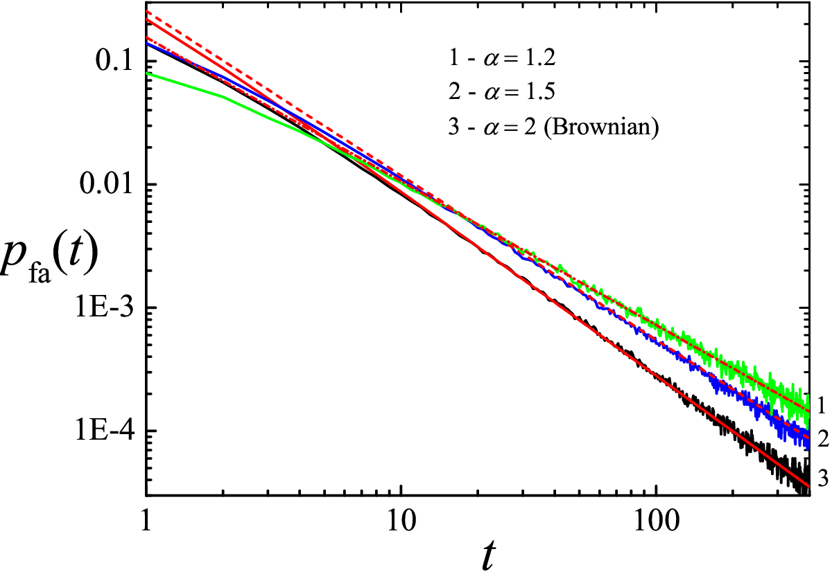
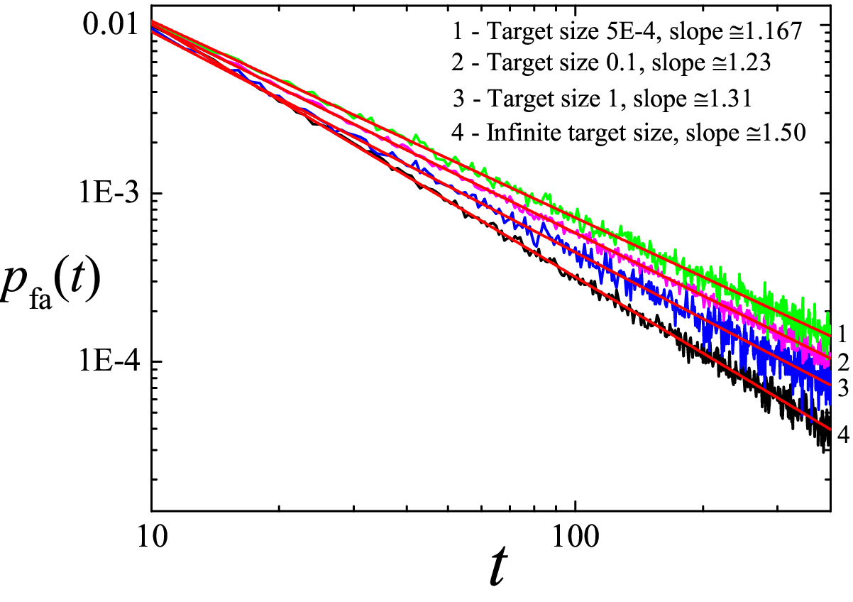
We briefly digress to address an important technical issue. A Brownian walker always explores the space continuously and therefore localizes any point on the line. However, in Langevin equation simulations, we introduce discrete (albeit small) jump lengths and time steps. Due to this, even for Brownian motion there is always a non-vanishing probability to overshoot a point-like target. Thus, even for the Brownian downhill case the simulated value of probability to eventually find the target becomes less than 1. This effect needs to be remedied by the appropriate choice of a finite target size. The tradeoff is now that the target needs to be sufficiently large to avoid the overshoot by the searcher. At the same time the target should not be too large, otherwise inconsistencies with our theory based on a point-like target would arise. The likelihood for leapovers across the target is naturally even more pronounced for the LF case. As a consistency test for the target size used in the simulations we check the long time asymptotics of the first arrival density against the analytical form given by Eq. (11). The results for this test are plotted in Fig. 2, showing excellent agreement between the simulations and the theoretical asymptotic behavior. In Fig. 3 we explicitly show the effect of a varying target size. As the target size is successively increased, the LF scaling of the first arrival density for a point-like target, , is seen to cross over to the universal Sparre-Andersen law for the first passage of a symmetric random walk process in the semi-infinite domain, [55, 49]. We see that it is possible to choose the target size appropriately such that the results of the Langevin equation simulations are consistent with the theory.
III First arrival and search efficiency in absence of an external bias
We first consider the case in absence of the bias and present the solution for the first arrival density. Moreover we motivate our choice for the efficiency used to compare different parameter values for the LF search process.
III.1 First arrival density and search reliability
Without external bias Eq. (7) can be expressed in terms of the Fox -function, as detailed in App. D. Inverse Laplace transform (62) of the -function allows us to obtain the solution (D) in the time domain. From the latter expression we get the long time asymptotic behavior of ,
| (11) |
where the constant is given by Eq. (66). In this way we find one of the central results of Ref. [49] by using the analytic approach of the -function formalism.
An important quantity for the following is the search reliability, defined as the cumulative arrival probability
| (12) |
It follows from Eq. (62) that without a bias , i.e. the searcher will always find the target eventually as long as . In other cases it will turn out that , that is, the searcher will not always locate the target no matter how long the search process is extended.
In the Brownian case , the -function in Eq. (62) according to App. E and G can be simplified to the well-known result for the first arrival in Laplace domain,
| (13) |
Note that in the Brownian case with finite variance of relocation lengths, the process of first arrival is identical to that of the first passage [49].
III.2 Search efficiency
How can one define a good measure for the efficiency of a search process? On a general level, such a definition depends on whether saltatory or cruise foraging is considered [54], or whether a single target is present in contrast to a fixed density of targets. For saltatory motion as considered herein a typical definition of the search efficiency is the ratio of the number of visited target sites over the total distance traveled by the searcher [54],
| (14) |
This definition works well when many targets with a typical inter-target distance are present. The mean number of steps taking in the search process is equivalent to the typical time over which the process is averaged. As we here consider the case of a single target, in a first attempt to define the efficiency we could thus reinterpret definition (14) as the mean time to reach the target and thus take , where now would correspond to the expectation . However, in contrast to the situation with a fixed target density, diverges for simple Brownian search on a line without bias [55].
For this reason we propose a different measure for the search efficiency, namely
| (15) |
Instead of the average search time, we average over the inverse search time. This can be shown to be a useful measure for situations when is both finite or diverging. Using the relation
| (16) |
it is straightforward to show that
| (17) |
As an example, consider the efficiency of a Brownian walker without bias. With Eq. (13) we find
| (18) |
where for this equation we restored dimensionality. This is the classical result for a normally diffusive process: increasing diffusivity of the searcher improves the search efficiency per unit time.
Below we demonstrate the robustness of the new characteristic for several concrete cases. We mention that the definition leads to contradictory results for the biased case, as well. This will be shown in the next section.
III.3 Search optimization
We now decree that a given search strategy is optimal when the efficiency of the corresponding search process is maximal. In our case of LF search we define the optimal search as the process with the value of the stable index for fixed initial condition and fixed bias velocity leads to the highest value of . As we will see, an optimal search defined by this criterion is not (always) the same as the most reliable process with maximal search reliability .
For LF search without an external drift the density of first arrival is given by Eq. (62). The search efficiency is obtained by integration it over ,
| (19) |
Thus the search efficiency decays quadratically with the initial searcher-target separation and, depending on the value of , may become non-monotonic. In the Brownian limit the efficiency is , consistent with the above result (18). In the Cauchy limit the efficiency drops to zero.

Fig. 4 shows the efficiency as function of the initial searcher-target distance , for fixed values of the power-law exponent . We observe a strong dependence on , the strongest variation being realized for the Brownian case with . For close initial distances () the Brownian strategy is the most efficient process. However, with increasing at first LFs with become more efficient than Brownian motion, and for the strategy with outperforms all the others. This behavior is expected as for longer initial separations the occurrence of long jumps increases with decreasing , and thus fewer steps lead the searcher closer to the target. For short initial separations the occurrence of long jumps would lead to leapovers and thus to a less efficient arrival to the target.
Due to the strong dependence on the initial searcher-target separation the efficiency between different strategies should be compared for a given value of . This will be done in the following. Additional insight can be obtained from the relative efficiency
| (20) |
for a given which is the ratio of the efficiency for some given exponent over the maximum efficiency for this initial separation for the corresponding value . In Fig. 5 we show this relative efficiency as function of the stable exponent of the jump length distribution. The value is obviously assumed at . Fig. 5 exhibits a very rich behavior. Thus, when the searcher is originally close to the target (here ) the Brownian strategy turns out to be the most efficient, and the functional form of is completely monotonic. For growing initial separation, however, the highest efficiency occurs for smaller values of . For instance, the maximum efficiency shifts from for to for . In particular, for large separations the optimal stable index approaches the value obtained earlier for different LF search scenarios [18, 40, 42, 43, 44, 45, 46].

The second striking observation is that for larger initial separations the dependence of on is no longer monotonic. An implicit expression for is obtained from the relation
| (21) |
The result can be phrased in terms of the implicit relation
| (22) |
Here denotes the digamma function. From this relation we can use symbolic mathematical evaluation to obtain the functional behavior of the optimal Lévy index as function of the initial searcher-target distance . The result is shown in Fig. 6. Two distinct phenomena can be observed: first, the behavior at long initial separations demonstrates the convergence of the optimal exponent to the Cauchy value . Second, the optimal search is characterized by an increasing value for when the initial separation shrinks, and we observe a transition at some finite value : for initial distances between searcher and target that are smaller than some critical value , Brownian search characterized by optimizes the search. In our dimensionless formulation, we deduce from the functional behavior in Fig. 6 that .


IV First arrival and search efficiency in presence of an external bias
We now consider the case when an external bias initially either pushes the searcher towards or away from the target, the downhill and uphill scenarios. In the uphill regime, we can understand that both the Brownian and the LF searcher may never reach to the target. However, as we will see, due to the presence of leapovers a LF searcher may also completely miss the target when we consider the downhill scenario.
IV.1 Search reliability
We can quantify to what extent a search process will ever locate the target in terms of the search reliability defined in Eq. (12). We obtain this quantity from the first arrival density. We start with the Brownian case for , for which the arrival density can be calculated explicitly (see App. E and Ref. [55] for the derivation). In the Laplace domain, it reads
| (23) |
where we again turned back to dimensional variables to see the explicit dependence on the diffusivity . Thus, in the downhill case with we find that due to the relation the search reliability will always be unity, : in the downhill case the Brownian searcher will always hit the target. In the opposite, uphill case with , the result
| (24) |
for the search reliability has the form of a Boltzmann factor () and exponentially suppresses the location of the target. In this Brownian case we can therefore interpret as the probability that the thermally driven searcher crosses an activation barrier of height .
For the general case of LFs we obtain from Eq. (7) via change of variables the Laplace transform
| (25) |
of the first arrival density, where we use the abbreviation
| (26) |
In expression (25) we introduced the generalized Péclet number for the case of LFs,
| (27) |
In the Brownian limit and after reinstating dimensional units we recover the standard Péclet number , where the factor two is a matter of choice [55].


In Fig. 7 we depict the functional behavior of the search reliability for four different values of the Lévy index including the Brownian case . The cumulative probability depends only on the generalized Péclet number, as can be seen from expression (25) when we take the relevant limit . In both panels of Fig. 7 the left semi-axes with negative values correspond to the downhill case, in which the searcher is initially advected in direction of the target, while the right semi-axes pertain to the uphill scenario. The continuous lines correspond to the numerical solution of Eq. (7), and the symbols represent results based on Langevin equation simulations. In these simulations the values of the search reliability were obtained as a ratio of the number of searchers that eventually located the target over the overall number of the released 10,000 searchers. To estimate the error of the simulated value for the search reliability, we calculated for each consecutive 1000 runs and then determined the standard deviation of the mean value of these 10 results.
According to Fig. 7 for the case of uphill search the search reliability is worst for the Brownian walker and improves continuously for decreasing value of the stable index . This is due to the activation barrier (24) faced by the Brownian walker. For LFs this barrier is effectively reduced due to the propensity for long jumps. The reduction of the resulting jump length , where is the typical duration of a single jump, becomes more and more insignificant for increasing jump lengths . This is why the efficiency continues to improve until the Cauchy case is reached. Quantitatively, however, we realize that for increasing generalized Péclet number even for LFs the value of the search reliability quickly decreases to tiny values, and that the absolute difference between the different search strategies is not overly significant.
In the downhill case Fig. 7 demonstrates that the Brownian searcher will always locate the target successfully and thus return in agreement with previous findings [55]. In contrast, the search reliability decreases clearly with growing magnitude . This decrease worsens with decreasing stable exponent . The reason for this is the growing tendency for leapovers of LFs with decreasing . Once the LF searcher overshoots the target, it is likely to drift away quickly from the target and never return to its neighborhood. Overall, the functional dependence of on the generalized Péclet number becomes non-trivial once . From Fig. 7 we conclude that if the main criterion for the search is the eventual location of the target, that is, a maximum value of the search reliability , without prior knowledge the gain for a Brownian searcher in the downhill case is higher than the loss in the opposite case: if we do not know the relative initial position to the target, the Brownian search algorithm will on average be more successful.
In Fig. 8 we now turn to the dependence of the search efficiency on the Lévy index for fixed magnitude of the external bias . In each case we display the behavior for three different values of the initial distance between searcher and target. In the downhill scenario we observe a remarkable non-monotonic behavior for larger value for . Namely, the search efficiency drops when gets smaller than the Brownian value , for which . While for the small initial separation this drop is continuous, for the larger values of this trend is turned around, and the search efficiency grows again. Due to the extremely slow convergence of both the Langevin equation simulations and the numerical evaluation of Eq. (7) despite all efforts we were not able to infer the continuation of the -curve for -values smaller than and thus, in particular, what the limiting value at the Cauchy case is. What could be the reason for this non-monotonicity in the versus dependence? Similar to the existence of an optimal -value intermediate between the Brownian and Cauchy cases and , respectively, for the search reliability we here find a worst-case value for . This value represents a negative tradeoff of the target overshoot property and insufficient propensity to produce sufficiently long jumps to recover an accumulated activation barrier from a downstream location as seen from the target. In the uphill case the dependence is monotonic: here long jumps become helpful to overcome the activation towards the target. Thus the search efficiency increases when becomes smaller and approaches the Cauchy value . The value for significantly drops with increasing value of the initial searcher-target separation . Consistently with the previous observations on the Brownian case fares worst and leads to the smallest value of .
IV.2 Search efficiency
For a Brownian searcher in the presence of an external bias, the mean search time can be computed via
| (28) |
For the downhill case this value is given by the classical result
| (29) |
The diffusing searcher moves towards the target as if it were a classical particle, the search time being given as the ratio of the distance over the (drift) velocity. It is independent of the value of the diffusion constant. For the uphill case (), we find the known result
| (30) |
The latter value is in fact smaller than the one for the downhill case. How can this be? The explanation of this seeming paradox comes from the qualitative difference in the nature of these averages. In the first scenario the search reliability is unity, that is, the walker always arrives at the target. In the uphill case only successful walkers count, that is, the average is conditional. This explains the seeming contradiction with common sense [56]. As we can see from this discussion is that the ready choice as a measure for the search efficiency would state that the uphill motion is more efficient than the downhill one. This definition would obviously not make much sense. We show that our definition of the search efficiency, Eq. (15), is a reasonable measure in this case. With the use of Eqs. (17) and (23) we find
| (31) |
Indeed, we see that our expression for the efficiency shows that the downhill motion is more efficient than going uphill for the same initial separation .


In Figs. 9 and 10 the efficiency is plotted for different values of the drift velocity and the initial separation of searcher and target, respectively. As expected, the increase of the downhill velocity leads to an efficiency growth, and vice versa for the opposite case. By magnitude of the -dependence, the decrease in the search efficiency for the uphill case is much more pronounced than the increase in efficiency for the downhill case. Hence, the dependence on the initial distance becomes increasingly asymmetric.
IV.3 Weak bias expansion for Lévy flight search
In the limit of a weak external bias we can obtain analytical approximations for the search efficiency. Namely, for sufficiently small values of the generalized Péclet number and nonzero values of the Laplace variable the denominators in both integrals of Eq. (25) can be expanded into series. The first order expansion reads
| (32) |
where we define
| (33) |
The integrals appearing in expression (32) can be computed by use of the Fox -function technique, as detailed in App. F. From the result (F) we obtain the following expression for the search efficiency,
| (34) |
where the first term in the square brackets corresponds to the result for the case without drift (), Eq. (19). When , the Brownian behavior in the small bias limit is recovered, namely, , consistent with the small expansion of Eq. (31)). From Eq. (F) it follows that for the Brownian case , the first arrival density in the Laplace domain has the approximate form
| (35) |
which is valid for , i.e., for short times. After transforming back to the time domain, we find
| (36) |
as shown in App. E. This result corresponds to the short time and small Péclet number limit of the general expression for reported by Redner [55]. Thus our expansion (F) works only at short times. However, the approximate expression (34) for the search efficiency itself turns out to work remarkably well, as shown in Fig. 11. Here, the behavior described by Eq. (34) is compared with results of direct numerical integration of Eq. (7) over . We see an almost exact match for an initial searcher-target separation . Instead, for the agreement becomes worse (not shown here). The explanation is due to the fact that for small initial separations short search times dominate the arrival statistic, while for the arrival is shifted to longer times, and the approximation underlying Eq. (34) does no longer work well.

The presence of an external bias substantially changes the functional form of the efficiency as compared to the unbiased situation. Fig. 12 shows the search efficiency as function of the initial position for two different drift velocities and for a variety of values of the power-law exponent . As expected from what we said before, the dependencies of the search efficiency with respect to positive and negative initial separations is asymmetric, as this corresponds to the difference between uphill and downhill cases elaborated above. Increasing magnitude of the bias effects a more pronounced asymmetry between values with the same absolute value . For the downhill case the advantage of the Brownian search over LF search persists for all values of . As expected, the efficiency drops, however, the general behavior is similar for all values. For the uphill case we observe a remarkable crossing of the curves. For small initial separations the Brownian search efficiency is highest. Here the activation barrier is sufficiently small such that the continuous Brownian searcher without leapovers locates the target most efficiently. When goes to increasingly negative values, successively LFs with smaller values become more efficient. In terms of the efficiency we see that for sufficiently large barriers, that is, when the target is initially separated by a considerable uphill distance from the searcher, LFs with smaller fare dramatically better than processes with larger .


We further illustrate the behavior of the search efficiency by studying its functional dependence on the stable index for different initial distances between searcher and target as well as for different drift velocities in Fig. 13. Thus, for short initial separation shown in Fig. 13 on the left, the Brownian searcher is always the most efficient for all cases: unbiased, downhill, and uphill. For larger as shown in the right panel of Fig. 13, the situation changes: in the downhill case the Brownian searcher still fares best. However, already in the unbiased case the LF searchers produce a higher efficiency. An interesting fact is the non-monotonicity of the behavior of the search efficiency, leading to an optimal value for the stable index , whose value depends on the strength of the bias (and the initial separation ). This is shifting towards the Cauchy value for increasing uphill bias.
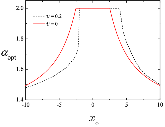
We can also find a qualitative argument for the optimal value of the power-law index in the small bias limit. If we denote , then . In comparison to the unbiased case, that is, the efficiency is reduced in the uphill case and increased in the downhill case, as it should be. Moreover, the correction due to the bias is more pronounced for larger values of . Hence the optimal necessarily shifts to larger values for the downhill case in comparison with the unbiased situation, and vice versa in the uphill case.
This can be perfectly illustrated with Fig. 14. The plot shows that application of a bias apparently breaks a symmetry in terms of initial position of a searcher: optimal values increase for downhill side and drop for uphill side. Thus, the range of values where the Brownian motion is optimal is effectively shifted.
IV.4 Implicit formula for the first arrival density
We briefly mention a different way to approach the first arrival problem in terms of an implicit expression for the corresponding density . From Eq. (7), by inverse Laplace transform we find
| (37) |
With the functions defined in App. H, we rewrite this relation in the form
| (38) |
such that we arrive at the simple form
| (39) |
in terms of the Laplace transforms . This is a familiar form for the first passage density for continuous processes [55], and is also known for the first arrival of LFs [49]. For numerical evaluation or small bias expansions this expression turns out to be useful.
V Discussion
We generalized the prominent Lévy flight model for the random search of a target to the case of an external bias. This bias could represent a choice of the searcher due to some prior experience, a bias in an algorithmic search space, or simply an underwater current or airflow. To compare the efficiency of this biased LF search for different initial searcher-target separations and values of the external bias, we introduced the search efficiency in terms of the mean of the inverse search time, . We confirmed that this measure is meaningful and in fact more consistent than the traditional definition in terms of the inverse mean search time, . As a second measure for the quality of the search process we introduced the search reliability, the cumulative arrival probability. When this measure is unity, the searcher will ultimately always locate the target. When it is smaller than unity, the searcher has a finite chance to miss the target. As shown here, high search reliability does not always coincide with a high search efficiency. Depending on what we expect from a search process, either measure may be more relevant.
In terms of the efficiency we saw that even in absence of a bias the optimal strategy crucially depends on the initial separation between the searcher and the target. For small the Brownian searcher is more efficient, as it cannot overshoot the target. With increasing , however, the LF searcher needs a smaller number of steps to locate the target and thus becomes more efficient. In the presence of a bias there is a strong asymmetry depending on the direction of the bias with respect to the initial location of the searcher and the target. For the downhill scenario the Brownian searcher always fares better, as it is advected straight to the target while the LF searcher may dramatically overshoot the target in a leapover event and then needs to makes its way back to the target, against the bias. The observed behaviors can be non-monotonic, leading to an optimal value for the power-law exponent . For strong uphill bias and large initial separation the optimal value is unity, for short separations and downhill scenarios the Brownian limit is best. There exist optimal values for in the entire interval , depending on the exact parameters.
The search reliability for a given value of solely depends on the generalized Péclet number. For unbiased search the searcher will always eventually locate the target, that is, the search efficiency attains the value of unity. In the presence of a bias, unity is returned for the search reliability for a Brownian searcher in the downhill case. It decays exponentially for the uphill case. For LF searchers with smaller than two, the probability of leapovers reduces the value of the search reliability in the downhill case. In the opposite, uphill scenario the search reliability is larger for LF searchers compared to the Brownian searcher. The absolute gain in this case, however, was found to be smaller than the loss to a Brownian competitor in the downhill case. Without prior knowledge of the bias a Brownian search strategy may turn out to be overall advantageous. We also found a non-monotonicity of the search reliability as function of the initial searcher-target separation . It will be interesting to see whether our results for both the search efficiency and reliability under an external bias turn out similarly for periodic boundary conditions relevant for finite target densities.
We note here that we analyzed LF search in one spatial dimension. What would be expected if the search space has more dimensions? For regular Brownian motion we know that it remains recurrent in two dimensions, that is, the sample path is space-filling in both one and two dimensions. On the other hand LFs with are recurrent in one dimension but always transient in two dimensions. Hence in two dimensions LFs will even more significantly reduce the oversampling of a Brownian searcher. At the same time, however, the search reliability will go to zero. In both one and two dimensions (linearly or radially) LFs are distinct due to the possibility of leapovers, owing to which the target localization may become less efficient than for Brownian search. Many search processes indeed fall in the category of (effectively) one or two dimensions. For example, they are one-dimensional in streams, along coastlines, or at forest-meadow and other borders. For (relatively) unbounded search processes as performed by birds or fish, the motion in the vertical dimension shows a much smaller span than the radial horizontal motion, and thus becomes effectively two dimensional. If we modify the condition of blind search and allow the walker to look out for prey while relocating, in one dimension this would obviously completely change the picture in favor of LFs with their long unidirectional steps. However, in two dimensions the radial leapovers would still impede the detection of the target unless it is exactly crossed during a step.
So what remains of the LF hypothesis? Conceptually, it is certainly a beautiful idea: a scale-free process reduces oversampling and thus scans a larger domain. If the target has an extended width, for instance, a large school instead of a single fish, LFs will then optimize the search under certain criteria. However, even when the stable index is larger than unity, in two or three dimensions an LF may also never reach the target, due to its patchy albeit scale-free exploration of the search space. Thus, even under LF-friendly conditions such as extremely sparse targets and/or uphill search, the superiority of LFs over other search models depends on the exact scenario. For instance, whether it is important that the target is eventually located with certainty, or whether in an ensemble of equivalent systems only sufficiently many members need a quick target localization, for instance, the triggering of some gene expression process responding to a lethal external signal in the cells of a biofilm. The LF hypothesis even in the case of blind search without any prior knowledge is therefore not universal, and depending on the conditions of initial searcher target separation or the direction of a naturally existing gradient with respect to the location of the target the regular Brownian motion may be the best search strategy.
LFs are most efficient under the worst case conditions of blind search for extremely sparse targets and, as shown here, for uphill motion. While very rare targets certainly exist in many scenarios, we should qualify the result for the uphill motion. The above uphill LF scenario holds for abstract processes such as the blind search of computer algorithms in complex landscapes or for the topology-mediated LFs in models of gene regulation. For the search of animals moving against a physical air or water stream, however, we have to take into consideration that any motion against a gradient requires a higher energy expenditure. Unless the gradient is very gentle, this aspect relativizes the LF hypothesis further.
Having said all this, one distinct advantage of spatially scale free search processes remains. Namely, they are more tolerant to gradually shifting environmental conditions, for instance, a change in the target distribution, or when the searcher is exposed to a new patch with conditions unknown to him. This point is often neglected in the analysis of search processes. A more careful study of this point may in fact turn back the wheel in favor of LF search.
It should be noted that LFs are processes with a diverging variance , and may therefore be considered unphysical. There exists the closely related superdiffusive model of Lévy walks, they have a finite variance due to a spatiotemporal coupling introducing a finite travel velocity, compare, for instance, Ref. [57]. This coupling penalizes long jumps. However, both models converge in the sense that the probability density function of a Lévy walker displays a growing Lévy stable portion in its center, limited by propagating fronts. The trajectory of such a Lévy walk appears increasingly similar to an LF: local search interspersed by decorrelating long excursions. We expect that at least qualitatively our present findings remain valid for the case of Lévy walks. It will be interesting to investigate this quantitative statement in more detail.
Acknowledgements.
VVP wishes to acknowledge financial support from Deutsche Forschungsgemeinschaft (Project no. PA 2042/1-1) as well as discussions with J. Schulz about simulation of random variables, A. Cherstvy for help with numerical methods in Mathematica and R. Klages for pointing out Ref. [54]. RM acknowledges support from the Academy of Finland within the FiDiPro scheme. AVCh acknowledges DAAD for financial support.Appendix A Derivation of dimensionless Eq. (3)
We here show how to consistently introduce dimensionless units in the fractional Fokker-Planck equation. If we denote the dimensionless time and position coordinate respectively by and , such that and with the dimensional parameters and defined below. Then we can rewrite Eq. (2) in the form
| (40) |
Note that we are dealing with dimensional density functions so that
| (41) |
and thus
| (42) |
Equation (40) then assumes the form
| (43) | |||||
where . We choose the parameters and as
| (44) |
where and correspond to the scaling factors of the jump length and waiting time distributions of the continuous time random walk. These appear in the Fourier and Laplace transforms of the jump length and waiting time densities [15]. The respective expansions used in the derivation of the continuous time random walk model for Lévy flights are
| (45) |
The diffusion coefficient in the fractional Fokker-Planck equation is then expressed in terms of these parameters as [15, 58]
| (46) |
We thus obtain the dimensionless dynamic equation (3).
Appendix B Proof that for and
To obtain the search reliability via the relation one first integrates Eq. (7) over and then takes the limit . If and , both integrals in the numerator and denominator of Eq. (7) converge. In this and the next appendices we prove that for and . Hence , which means that the searcher never reaches the target in the case .
Taking in Eq. (7) we have
| (47) |
For the integral in the denominator diverges at infinity. Let us consider the integral in the numerator. We notice that
| (48) |
for . Thus the numerator of expression (47) converges for . Since the denominator diverges in this range, for all values of . Thus, the search reliability vanishes, , and the searcher never reaches its target. The limiting case needs separate attention. We observe that the integral (48) diverges. For ,
| (49) |
expression for . The integrals are
| (50) |
which logarithmically diverges for , and
| (51) | |||||
The second term in Eq. (51) converges. Thus, in the ratio over the divergent integral (50) it can be neglected. The first term can be modified to
| (52) | |||||
When the second term in Eq. (52) is the cosine integral at , and it vanishes. Altogether, for any finite
| (53) |
which completes the proof.
Appendix C Proof that for and
Let us start from the Cauchy case . The expression for the first arrival density follows from Eq. (7),
| (54) |
with
| (55) |
Alternatively,
| (56) |
Let us first consider the integral in the denominator,
| (57) |
At only the first term is significant, and it diverges logarithmically. The integral in the numerator converges due to the oscillating functions in the integrands. With the diverging denominator and the converging numerator in Eq. (56), we have that for any finite . The search reliability vanishes.
For in Eq. (7) with we have , and the proof is analogous to the case just considered.
Appendix D Solution for via Fox -functions
Without a bias, Eq. (7) takes on the form
| (58) |
where the abbreviation is defined in Eq. (33). The integral in the denominator yields [59]
| (59) |
The integral in the numerator can be obtained in terms of the Fox -function technique [60]. Since
| (60) |
we find that
| (61) |
where we used Eq. (60) and the integral (2.25.2.4) from Ref. [59]. Transforming the -function by help of the properties (1.3) and (1.5) from Ref. [60] we obtain
| (62) |
Using the properties of the Laplace transform of the -function (see chapter 2 in Ref. [60]) we get the first arrival density in the time domain,
Expansion of Eq. (D) in the long-time limit yields Eq. (11), where
| (66) |
Appendix E General solution for the Brownian case
It is instructive to obtain the well-known first arrival density in the Brownian case directly from Eq. (7). For , Eq. (7) assumes the form
| (67) |
where
| (68) |
The denominators in these integrals are quadratic polynomials in and hence can be rewritten as , where
| (69) |
Then both integrals can be easily calculated by the method of residues, and we arrive at Eq. (23).
Appendix F Expansion (32) in terms of -functions
We show here how expansion (32) is obtained in terms of -functions. Two out of three integrals in Eq. (32) were computed above in App. D as Eqs. (59) and (61). The last unknown integral from expression (32) can be computed in a similar way,
With these results we obtain the following expression in Laplace space,
Inverse Laplace transform of Eq. (F) yields
Appendix G Derivation of the Brownian weak bias expansion (F)
We represent the first arrival density from Eq. (F) as , where the first and second contribution correspond to the first and second terms in the expression (F). Then for the order of -function is reduced by use of the properties 1.2 and 1.3 from chapter 1 in Ref. [60]) as well as its definition via the Mellin transform [60]. This procedure yields
Similar steps for lead to the result
Thus , which is the expansion of the general solution in the Brownian case, expression (70). The same result can be obtained by calculations in -space
and
Appendix H Implicit Fox -function expression for
The expressions for and in Eq. (37) can be obtained by help of standard properties of -function [59] and the identification for the exponential function,
| (111) |
Consequently,
and
To construct the expression (39) for the first arrival density, we need the Laplace transforms of the functions . For we find
Using the expansion of the -function at small arguments [60] we find at
| (126) |
which is exactly the same result as one can get by direct computation of the integral and subsequent Laplace transform.
At from Eq. (H) we get by direct Laplace transform
and hence
We see that this expression is different from Eq. (62) in the order of the first two brackets in the top row of the -function. However, these brackets can be exchanged due to property 1.1 of the -function in Ref. [60]. Thus, the -function solution for the unbiased case () is obtained correctly.
Now let us derive the result for any in the limit . For that purpose we note that
For the reduction formula for -functions (property 1.2 of Ref. [60]) yields
| (141) |
where we restored the Brownian diffusivity. Alternatively,
| (142) |
Since ,
| (143) |
Inverse Laplace transform of the latter relation produces Eq. (73).
References
- [1] O. Bénichou, C. Loverdo, M. Moreau and R. Voituriez, Rev. Mod. Phys. 83, 81 (2011).
- [2] P. C. Bresloff and J. M. Newby, Rev. Mod. Phys. 85, 135 (2013).
- [3] J. Elf, G. W. Li, and X. S. Xie, Science 316, 1191 (2007); P. Hammar et al, ibid. 336, 1595; M. Bauer and R. Metzler, PLoS ONE 8, e53956 (2013); O. Pulkkinen and R. Metzler, Phys. Rev. Lett. 110, 198101 (2013); T. E. Kuhlman and E. C. Cox, Mol. Syst. Biol. 8, 610 (2012).
- [4] R. Nathan, W. M. Getz, E. Revilla, M. Holyoak, R. Kadmon, D. Saltz, and P. E. Smouse, Proc Natl Acad Sci USA 105, 19052 (2008).
- [5] G. E. Viswanathan, M. G. E. da Luz, E. P. Raposo, and H. E. Stanley, The Physics of Foraging. An Introduction to Random Searches and Biological Encounters (Cambridge University Press, New York, NY, 2011).
- [6] I. Pavlyukevich, J. Comput. Phys. 226, 1830 (2007).
- [7] A. James, J. W. Pitchford, and M. J. Plank, Bull. Math. Biol. 72, 896 (2010).
- [8] D. W. Sims et al., Nature 451, 1098 (2008).
- [9] N. E. Humphries et al., Nature 465, 1066 (2010).
- [10] J. F. Burrow, P. D. Baxter, and J. W. Pitchford, Math Model Nat Phenom 3, 115 (2008).
- [11] D.W Sims, M.J Witt, A.J. Richardson, E.J. Southall and J.D. Metcalfe, Proc. R. Soc. B, 273, 1195 (2006).
- [12] J.D.R. Houghton, T.K. Doyle, M.W. Wilson, J. Davenport, and G.C. Hays, Ecology, 87, 1967 (2006).
- [13] C.J.A. Bradshaw, M.A. Hindell, M.D. Sumner, and K.J. Michael, Animal Behaviour, 68, 1349 (2004).
- [14] M. F. Shlesinger and J. Klafter in On Growth and Form, edited by H. E. Stanley and N. Ostrowsky (Martinus Nijhoff, Dordrecht, 1986).
- [15] R. Metzler and J. Klafter, Phys. Rep. 339, 1 (2000); J. Phys. A 37, R161 (2004).
- [16] B. D. Hughes, Random Walks and Random Environments, Vol. I: Random Walks (Oxford University Press, Oxford, UK, 1995).
- [17] M. Vahabi, J. H. P. Schulz, B. Shokri, and R. Metzler, Phys. Rev. E 87, 042136 (2013).
- [18] G. M. Viswanathan, S. V. Buldyrev, S. Havlin, M. G. E. da Luz, E. P. Raposo and H. E. Stanley, Nature, 401, 911 (1999).
- [19] F. Bartumeus, J. Catalan, U. L. Fulco, M. L. Lyra, and G. M. Viswanathan, Phys. Rev. Lett. 88, 097901 (2002).
- [20] G.M. Viswanathan, V. Afanasyev, S.V. Buldyrev, E.J. Murphy, P.A. Prince and H.E. Stanley, Nature ,381, 413 (1996).
- [21] D.W. Sims et al., Nature, 451 1098 (2008)
- [22] N.E. Humphries et al., Nature, 465 1066 (2010).
- [23] A. M. Reynolds, D. R. Reynolds, A. D. Smith, G. P. Svensson, and C. Löfstedt, J Theor Biol, 245, 141 (2007).
- [24] S. Focardi, P. Montanaro, E. Pecchioli, PLoS One 4, e6587 (2009).
- [25] H. J. de Knegt, G.M. Hengeveld, F. van Langevelde, W. F. de Boer, and K. P. Kirkman, Behav Ecol 18, 1065 (2007).
- [26] F. Bartumeus, F. Peters, S. Pueyo, C. Marrasé, and J. Catalan, PNAS, 100, 12771 (2003).
- [27] D. Boyer, G. Ramos-Fernández, O. Miramontes, J. L. Mateos, G. Cocho, H. Larralde, H. Ramos, and F. Roja, Proc Biol Sci., 273, 1743 (2006).
- [28] V. A. A. Jansen, A. Mashanova, and S. Petrovskii, Science, 335 918 (2012).
- [29] A. Mashanova, T. H. Oliver, and V. A. A. Jansen, J. Roy. Soc. Interface, 7, 199 (2010).
- [30] S. Petrovskii, A. Mashanova, and V. A. A. Jansen, Proc. Natl. Acad. USA 108, 8704 (2011).
- [31] A. M. Edwards et al., Nature 449, 1044 (2007).
- [32] N. E. Humphries, H. Weimerskirch, N. Queiroza, E. J. Southalla, and D. W. Sims, Proc. Natl. Acad. Sci. USA 109, 7169 (2012).
- [33] D. Brockmann, Phys. World, 2, 31 (2010).
- [34] D. Brockmann, L. Hufnagel, and T. Geisel, Nature, 439, 462 (2006).
- [35] C. Song, T. Koren, P. Wang, and A.L. Barabási, Nature Physics 6, 818 (2010).
- [36] S. Bertrand, J.M. Burgos, F. Gerlotto, and J. Atiquipa, ICES Journal of Marine Science, 62 477 (2005).
- [37] A. M. Edwards, Ecology 92, 1247 (2011).
- [38] M. van Dartel, E. Postma, J. van den Herik, G. de Croon, Connection Science, 16 169 (2004).
- [39] O. Bénichou, M. Coppey, M. Moreau, P. H. Suet, and R. Voiturierz, Phys. Rev. Lett. 94, 198101 (2005); C. Loverdo, O. Bénichou, M. Moreau, and R. Voiturierz, Nature Phys. 4, 134 (2008); compare also S. Benhamou, Ecology 88, 1962 (2007); A. Reynolds, Physica A 388, 561 (2009).
- [40] M. A. Lomholt, T. Koren, R. Metzler, and J. Klafter, Proc. Natl. Acad. Sci. USA 105, 11055 (2008).
- [41] P. Bovet and S. Benhamou, J. Theoret. Biol. 131, 419 (1988).
- [42] M. A. Lomholt, T. Ambjörnsson, and R. Metzler, Phys. Rev. Lett. 85, 260603 (2005).
- [43] F. Bartumeus, M. G. E da Luz, G. M. Viswanathan, and J. Catalan, Ecology 86, 3078 (2005).
- [44] F. Bartumeus and S. A. Levin, Proc. Natl. Acad. Sci. USA 105, 19072 (2008).
- [45] A. M. Reynolds, Europhys. Lett. 82, 20001 (2008).
- [46] A. M. Reynolds, J. Phys. A 42, 434006 (2009).
- [47] V. V. Palyulin, A. V. Chechkin, and R. Metzler, Proc. Natl. Acad. Sci. USA, 111, 2931 (2014).
- [48] T. Koren, M. A. Lomholt, A. V. Chechkin, J. Klafter, and R. Metzler, Phys. Rev. Lett. 99, 160602 (2007). T. Koren, A. V. Chechkin, and J. Klafter, Physica A 379, 10 (2007).
- [49] A. V. Chechkin, R. Metzler, V. Yu. Gonchar, J. Klafter, and L.V. Tanatarov, J. Phys. A 36, L537 (2003).
- [50] A. V. Chechkin and V. Yu. Gonchar, J. Eksper. Theor. Phys. 91, 635 (2000).
- [51] K.-I. Sato, Lévy processes and infinitely divisible distributions (Cambridge University Press, Cambridge, UK 1999).
- [52] A. V. Chechkin, O. Yu. Sliusarenko, R. Metzler, and J. Klafter, Phys Rev. E 75 041101 (2007); O. Yu. Sliusarenko, V. Yu. Gonchar, A. V. Chechkin, I. M. Sokolov, and R. Metzler, ibid. 81, 041119 (2010).
- [53] J. M. Chambers, C. L. Mallows, and B. W. Stuck, J. Amer. Statist. Assoc. 71, 340 (1976).
- [54] A. James, J. W. Pitchford, and M. J. Plank, Bull. Math. Biol. 72, 896 (2010).
- [55] S. Redner, A Guide to First-Passage Processes (Cambridge University Press, Cambridge, UK, 2001).
- [56] V. I. Tikhonov and M. A. Mironov, Markov processes (Sov. Radio, Moscow, 1977).
- [57] J. Klafter, A. Blumen, and M. F. Shlesinger, Phys. Rev. A 35, 3081 (1987).
- [58] R. Metzler, E. Barkai, and J. Klafter, Europhys. Lett. 46, 431 (1999).
- [59] A. P. Prudnikov, Y. A. Brychkov, and O. I. Marichev, Integrals and series (Gordon & Breach, New York, NY, 1990).
- [60] A. M. Mathai, R. K. Saxena, and H.J. Haubold, The -function, theory and applications (Springer, Berlin, 2010).