跳到论文正文
W Papers独立论文阅读器 arXiv:1402.2467 论文正文 计算阅读时间 · 0%
引用这篇论文根据当前论文元数据生成,正式投稿前建议核对。


License: arXiv.org perpetual non-exclusive license
arXiv:1402.2467v1 [math.OC] 11 Feb 2014

A model problem for Mean Field Games on networks11 1 This work is partially supported by European Union under the 7th Framework Programme FP7-PEOPLE- 2010-ITN Grant agreement number 264735-SADCO

Abstract

In [14], Guéant, Lasry and Lions considered the model problem “What time does meeting start?” as a prototype for a general class of optimization problems with a continuum of players, called Mean Field Games problems. In this paper we consider a similar model, but with the dynamics of the agents defined on a network. We discuss appropriate transition conditions at the vertices which give a well posed problem and we present some numerical results.

Fabio Camilli

“Sapienza” Università di Roma

Dip. di Scienze di Base e Applicate per l’Ingegneria

via Scarpa 16, 0161 Roma, Italy

e-mail:camilli@dmmm.uniroma1.it

Elisabetta Carlini

“Sapienza” Università di Roma

Dip. di Matematica

P.le A. Moro 5, 00185 Roma, Italy

e-mail:carlini@mat.uniroma1.it

Claudio Marchi

Università di Padova

Dip. di Matematica

via Trieste 63, 35121 Padova, Italy

email:marchi@math.unipd.it

MSC 2000:

91A15, 35R02, 35B30, 49N70, 65M06.

Keywords:

networks, mean field games, stochastic optimal control, numerical methods.

1 Introduction

The study of pedestrian flow in a crowd environment is attracting an increasing interest and some models based on optimization principles have been recently proposed, see for example [4, 8, 20]. In some applications (crowd motion in shopping centers, stations, airports) the dynamics of the population is defined on a network rather than in an Euclidean domain.
There is a large literature concerning vehicular traffic on road networks (see [11] and reference therein). These models are based on a fluido-dynamical approach with the dynamics described by some nonlinear conservation law and appropriate transition conditions at the junctions modelling the interactions of the cars coming from different roads. Vehicular traffic models do not seem to be adequate to reproduce the pedestrian flow since they do not take into account the interactions and the goal-directed decisions of the agents.
Aim of this paper is to study a simple optimization model for the evolution of a large number of agents moving on a network. The model is based on the one described in [14], titled “What time does meeting start?”, and consists in finding the optimal arrival time at a place where the meeting is being held with the starting time defined by means of a quorum rule. This problem can be considered as a prototype for a large class of optimization problems based on the Mean Field Game (MFG) theory. This theory has been introduced by Lasry and Lions [17] (see also [1], [6], [12]) with the aim of describing the behavior of very large number of agents who take decisions in a context of strategic interactions.
The main difficulties in our approach is to deal with the transition conditions at the internal vertices to obtain a well posed MFG problem. It is known that a parabolic equation on a network has to be complemented with the usual initial-boundary conditions and some transition conditions at the internal vertices (see [3, 18]). In fact, in our model the stochastic differential equation describing the motion of the agent inside the arcs is coupled with a condition prescribing the probability that it enter in a given edge when it occupies a transition vertex; this fact give rise to a Kirchhoff type condition (see [9]). Using an appropriate change of variable we transform the original MFG system in a forward-backward system of two heat equations coupled via the initial datum. Relying on classical results for the heat equation on networks and some appropriate estimates for the specific problem, we prove the well-posedness of the heat system and the existence of a mean field for the quorum problem.

Going back to the original MFG problem we obtain existence and uniqueness of the solution to a system composed by a backward Hamilton-Jacobi-Bellman equation and a forward Fokker-Planck on the arcs with transitions conditions expressing respectively the probability that a single agent enters a given arc and the conservation of the density of the agents through a vertex.

The paper is organized as follows. In Section 2 we describe the model problem. In 3 we prove some technical results concerning the heat equation on the network which are used in Section 4 to show the existence of the mean field. in Section 5, we illustrate the problem with some numerical examples. Finally, the Appendix contains some technical proofs.

Notations: A network is a finite collection of points V:={vi}i∈IV:=\{v_{i}\}_{i\in I} in ℝn{\mathbb{R}}^{n} connected by continuous, non self-intersecting arcs E:={ej}j∈JE:=\{e_{j}\}_{j\in J}. Each arc eje_{j} is parametrized by a smooth function πj:[0,lj]→ℝn,lj>0\pi_{j}:[0,l_{j}]\to{\mathbb{R}}^{n},\,l_{j}>0.
For i∈Ii\in I we set I​n​ci:={j∈J∣ej​is incident to​vi}Inc_{i}:=\{j\in J\mid\,e_{j}\,\text{is incident to}\,v_{i}\}. We denote by IB:={i∈I∣#​I​n​ci=1}I_{B}:=\{i\in I\mid\#Inc_{i}=1\}, IT:=I∖IBI_{T}:=I\setminus I_{B}, by ∂Γ:={vi∈V∣i∈IB}\partial\Gamma:=\{v_{i}\in V\mid\,i\in I_{B}\}, the set of boundary vertices of Γ\Gamma, and by ΓT:={vi∣i∈IT}\Gamma_{T}:=\{v_{i}\mid i\in I_{T}\}, the set of transition vertices.
The network is not oriented, but the parametrization of the arcs induces an orientation which can be expressed by the signed incidence matrix A={ai​j}A=\{a_{ij}\} with

ai​j:={1if vi∈ej and πj​(0)=vi,−1if vi∈ej and πj​(lj)=vi,0otherwise.a_{ij}:=\left\{\begin{array}[]{rl}1&\hbox{if $v_{i}\in e_{j}$ and $\pi_{j}(0)=v_{i}$,}\\ -1&\hbox{if $v_{i}\in e_{j}$ and $\pi_{j}(l_{j})=v_{i}$,}\\ 0&\hbox{otherwise.}\end{array}\right.

In the following we always identify x∈ejx\in e_{j} with y=πj−1​(x)∈[0,lj]y=\pi_{j}^{-1}(x)\in[0,l_{j}]. For any function u:Γ→ℝu:\Gamma\to{\mathbb{R}} and each j∈Jj\in J we denote by uj:[0,lj]→ℝu_{j}:[0,l_{j}]\to{\mathbb{R}} the restriction of uu to eje_{j}, i.e. uj​(y)=u⁡(πj​(y))u_{j}(y)=u(\pi_{j}(y)) for y∈[0,lj]y\in[0,l_{j}]. For γ∈ℕ\gamma\in{\mathbb{N}}, we define differentiation along an edge eje_{j} by

∂jγu⁡(x):=dγ​ujd​yγ​(y),for y=πj−1​(x), x∈ej\partial^{\gamma}_{j}u(x):=\frac{d^{\gamma}u^{j}}{dy^{\gamma}}(y),\qquad\text{for $y=\pi^{-1}_{j}(x)$, $x\in e_{j}$}

and at a vertex viv_{i} by

∂jγu⁡(vi):=dγ​ujd​yγ​(y)for y=πj−1​(vi), j∈I​n​ci.\partial^{\gamma}_{j}u(v_{i}):=\frac{d^{\gamma}u^{j}}{dy^{\gamma}}(y)\qquad\text{for $y=\pi^{-1}_{j}(v_{i})$, $j\in Inc_{i}$.}

2 The model problem

Following [14], we describe the model “What time does meeting start?” with the variant that the dynamics of the agents are defined on a network Γ\Gamma. For the sake of simplicity, we assume that the place where the meeting is being held is the unique boundary vertex, namely ∂Γ={v0}\partial\Gamma=\{v_{0}\}; the general case can be dealt with by using easy adaptations. The meeting is scheduled at a certain time t0t_{0} but the common experience says that in general it starts at a time TT greater than t0t_{0}, when a certain rule is reached, for example the presence of a certain percentage of participants.
At the initial time there is a continuum of indistinguishable players distributed according to a distribution function m0:Γ→ℝm_{0}:\Gamma\to{\mathbb{R}}. The player’s dynamics is subject to random perturbations. We assume that, inside each edge eje_{j}, the generic agent moves according to the process

d​X​(t)=a⁡(t)​d​t+σ​d​W​(t)dX(t)=a(t)dt+\sigma dW(t) (2.1)

where the drift aa is the control variable (and it coincides with the speed), σ=(σj)j∈J\sigma=(\sigma_{j})_{j\in J} with σj>0\sigma_{j}>0 and WW is a Brownian process, which is an independent disturbance for each player. Moreover we assume that, at each transition vertex viv_{i}, it spends zero time a.s. and it enters in one of the incident edge eje_{j} with probability 1/#⁡(I​n​ci)1/\#(Inc_{i}) (see [9, 10] for stochastic differential equations on networks). We denote by τ\tau the random time the agent reaches v0v_{0}, i.e.

τ:=inf{t>0:X⁡(t)∈∂Γ}.\tau:=\inf\{t>0:\,X(t)\in\partial\Gamma\}.

Moreover each player wants to optimize its arrival time τ\tau taking into account various parameters, which are encoded in the cost functional

J⁡(x,t,a⁡(⋅))=∫tτ∧Tm​a​x12​a2​(t)​𝑑t+c⁡(τ∧Tm​a​x)J(x,t,a(\cdot))=\int_{t}^{\tau\wedge T_{max}}\frac{1}{2}a^{2}(t)dt+c(\tau\wedge T_{max}) (2.2)

where 12​a2​(t)\frac{1}{2}a^{2}(t) is the actual cost of moving along the network at the velocity aa while cc is the final cost and Tm​a​x∈ℝT_{max}\in{\mathbb{R}} is a time which cannot be exceeded for the end of the meeting. The cost function c:[0,Tm​a​x]→ℝc:[0,T_{max}]\to{\mathbb{R}} is given by

c⁡(s)=c1​(s−t0)+c2​(s−T)+c3​(T−s),s∈[0,Tm​a​x]c(s)=c_{1}(s-t_{0})+c_{2}(s-T)+c_{3}(T-s),\qquad s\in[0,T_{max}] (2.3)

where ci:ℝ→ℝc_{i}:{\mathbb{R}}\to{\mathbb{R}}, i=1,2,3i=1,2,3 are smooth functions such that ci​(s)=0c_{i}(s)=0 for s≤0s\leq 0 and ci​(s)>0c_{i}(s)>0 for s>0s>0. The term c1​(s−t0)c_{1}(s-t_{0}) represents a reputation cost of lateness in relation to scheduled time t0t_{0}; the term c2​(s−T)c_{2}(s-T) a cost of lateness in relation to actual starting time of the meeting TT; c3​(T−s)c_{3}(T-s) a waiting time cost which corresponds to the time lost waiting the starting of the meeting. It is worth noticing that the cost cc depends on TT via the cost of lateness and the cost of waiting; hence, in order to display this dependence, from now on we write cTc_{T}.

Nash equilibrium theory assumes that each player want to optimize the arrival time by assuming that actual time TT the meeting starts is known. Hence each agent has to solve the optimization problem

u⁡(x,t)=mina⁡(⋅)⁡J⁡(x,t,a⁡(⋅))u(x,t)=\min_{a(\cdot)}J(x,t,a(\cdot)) (2.4)

where (x,t)∈Γ×[0,Tm​a​x](x,t)\in\Gamma\times[0,T_{max}]. Note that maxa∈ℝ⁡{−a​p+12​|a|2}=−12​|p|2\max_{a\in{\mathbb{R}}}\{-ap+\frac{1}{2}|a|^{2}\}=-\frac{1}{2}|p|^{2} for a=−pa=-p and the optimal control in feed-back form is given by a∗(x,t)=−∂xu(x,t)a^{*}(x,t)=-\partial_{x}u(x,t). By an application of the Dynamic Programming Principle the value function, if it is assumed to be regular, formally solves the Hamilton-Jacobi-Bellman equation

∂tu+ν​∂x2u+12​|∂xu|2=0(x,t)∈Γ×(0,Tm​a​x),\displaystyle\partial_{t}u+\nu\partial^{2}_{x}u+\frac{1}{2}|\partial_{x}u|^{2}=0\quad(x,t)\in\Gamma\times(0,T_{max}),

where ν=σ2/2\nu=\sigma^{2}/2 (i.e., νj=σj2/2∀j∈J\nu_{j}=\sigma_{j}^{2}/2\quad\forall j\in J), with final-boundary conditions and transition on internal vertices (Kirchhoff condition)

u⁡(x,Tm​a​x)=cT​(Tm​a​x)x∈Γ,u⁡(v0,t)=cT​(t)s∈[0,Tm​a​x],\displaystyle u(x,T_{max})=c_{T}(T_{max})\quad x\in\Gamma,\qquad u(v_{0},t)=c_{T}(t)\quad s\in[0,T_{max}],
∑j∈I​n​ciai​j​∂ju⁡(vi,s)=0(vi,s)∈ΓT×(0,Tm​a​x).\displaystyle\sum_{j\in Inc_{i}}a_{ij}\partial_{j}u(v_{i},s)=0\qquad(v_{i},s)\in\Gamma_{T}\times(0,T_{max}).

On the other hand, by duality, the dynamic of the agents, i.e. the evolution of the initial distribution m0m_{0}, is governed inside each edge by the Fokker-Planck equation

∂tm−ν∂x2m−∂x((−∂xu)m)=0(x,t)∈Γ×(0,Tm​a​x)\partial_{t}m-\nu\partial_{x}^{2}m-\partial_{x}((-\partial_{x}u)m)=0\quad(x,t)\in\Gamma\times(0,T_{max})

and we assume the initial-boundary condition (with a “smooth fit”) and a Kirchhoff condition on internal vertices

m⁡(x,0)=m0​(x)x∈Γ,m⁡(v0,s)=0s∈[0,T]\displaystyle m(x,0)=m_{0}(x)\quad x\in\Gamma,\qquad m(v_{0},s)=0\qquad s\in[0,T]
∑j∈I​n​ciai​j​νj​[∂jm−m​∂ju]​(vi,s)=0(vi,s)∈ΓT×(0,Tm​a​x).\displaystyle\sum_{j\in Inc_{i}}a_{ij}\nu_{j}[\partial_{j}m-m\partial_{j}u](v_{i},s)=0\qquad(v_{i},s)\in\Gamma_{T}\times(0,T_{max}).

Observe that the previous Kirchhoff condition implies that the parabolic flux of the agents is null at the junctions, giving the conservation of the total mass (see [7] for similar assumptions).

The flow of participants reaching v0v_{0} is given by s↦∂xm⁡(v0,s)s\mapsto\partial_{x}m(v_{0},s), hence the cumulative distribution FF of the arrival times is

F⁡(s)=∫0sν​∂xm⁡(v0,r)​𝑑r.F(s)=\int_{0}^{s}\nu\partial_{x}m(v_{0},r)dr.

The actual starting time TT is fixed by a quorum rule, which means that the meeting starts when a given percentage θ\theta of the participants has reached the meeting place v0v_{0}. Given mm, we set

T={t0,F−1​(θ)≤t0 F−1​(θ),t0<F−1​(θ)<Tm​a​xTm​a​x,F−1​(θ)≥Tm​a​x.T=\left\{\begin{array}[]{ll}t_{0},&\hbox{$F^{-1}(\theta)\leq t_{0}$ }\\[4.0pt] F^{-1}(\theta),&\hbox{$t_{0}<F^{-1}(\theta)<T_{max}$}\\[4.0pt] T_{max},&\hbox{$F^{-1}(\theta)\geq T_{max}$.}\end{array}\right. (2.5)

Note that TT is the mean field, i.e. the information that the single agent has about the behavior of the other agents: the starting rule induces a strategic interactions among the participants and TT influences as an external field the decisions of the agents. The main point is to prove the existence and the uniqueness of a time TT which is coherent with the expectations of the participants. As in [14], this can be done by proving that the scheme:

T→u→m→T∗T\rightarrow u\rightarrow m\rightarrow T^{*} (2.6)

with T∗T^{*} defined by (2.5), has a fixed point in [t0,Tm​a​x][t_{0},T_{max}]. To this end, it is important to study existence and uniqueness of a solution to the forward-backward system

{∂tu+ν​∂x2u+12​|∂xu|2=0(x,s)∈Γ×(0,Tm​a​x)∂tm−ν​∂x2m+∂x(∂xu​m)=0(x,s)∈Γ×(0,Tm​a​x)∑j∈I​n​ciai​j​∂ju⁡(vi,s)=0(vi,s)∈ΓT×(0,Tm​a​x)∑j∈I​n​ciai​j​νj​[∂jm−m​∂ju]​(vi,s)=0(vi,s)∈ΓT×(0,Tm​a​x)m⁡(x,0)=m0​(x),u⁡(x,Tm​a​x)=cT​(Tm​a​x)x∈Γm⁡(v0,s)=0,u⁡(v0,s)=cT​(s)s∈[0,Tm​a​x].\left\{\begin{array}[]{ll}\displaystyle\partial_{t}u+\nu\partial^{2}_{x}u+\frac{1}{2}|\partial_{x}u|^{2}=0&(x,s)\in\Gamma\times(0,T_{max})\\[6.0pt] \partial_{t}m-\nu\partial^{2}_{x}m+\partial_{x}(\partial_{x}u\,m)=0&(x,s)\in\Gamma\times(0,T_{max})\\[6.0pt] \sum_{j\in Inc_{i}}a_{ij}\partial_{j}u(v_{i},s)=0&(v_{i},s)\in\Gamma_{T}\times(0,T_{max})\\[6.0pt] \sum_{j\in Inc_{i}}a_{ij}\nu_{j}[\partial_{j}m-m\partial_{j}u](v_{i},s)=0&(v_{i},s)\in\Gamma_{T}\times(0,T_{max})\\[6.0pt] m(x,0)=m_{0}(x),\,u(x,T_{max})=c_{T}(T_{max})&x\in\Gamma\\[6.0pt] m(v_{0},s)=0,\,u(v_{0},s)=c_{T}(s)&s\in[0,T_{max}].\end{array}\right. (2.7)

For the sake of simplicity, from now on we assume

νj=1∀j∈I​n​ci.\nu_{j}=1\qquad\forall j\in Inc_{i}. (2.8)

As in [14, 15] we apply a change of variable which transforms system (2.7) into a forward-backward system of heat equations coupled through the initial conditions.

Proposition 2.1

If (ϕ,ψ)(\phi,\psi) is a smooth solution of the system

{−∂tϕ−∂2xϕ=0(x,s)∈Γ×(0,Tm​a​x),∂tψ−∂x2ψ=0(x,s)∈Γ×(0,Tm​a​x)∑j∈I​n​ciai​j​∂jϕ⁡(vi,s)=0(vi,s)∈ΓT×(0,Tm​a​x)∑j∈I​n​ciai​j​∂jψ⁡(vi,s)=0(vi,s)∈ΓT×(0,Tm​a​x)ψ⁡(x,0)=m0​(x)ϕ⁡(x,0),ϕ⁡(x,Tm​a​x)=ecT​(Tm​a​x)x∈Γψ⁡(v0,s)=0,ϕ⁡(v0,s)=ecT​(s)s∈[0,Tm​a​x]\left\{\begin{array}[]{ll}-\partial_{t}\phi-\partial^{2}_{x}\phi=0&(x,s)\in\Gamma\times(0,T_{max}),\\[6.0pt] \partial_{t}\psi-\partial^{2}_{x}\psi=0&(x,s)\in\Gamma\times(0,T_{max})\\[6.0pt] \sum_{j\in Inc_{i}}a_{ij}\partial_{j}\phi(v_{i},s)=0&(v_{i},s)\in\Gamma_{T}\times(0,T_{max})\\[6.0pt] \sum_{j\in Inc_{i}}a_{ij}\partial_{j}\psi(v_{i},s)=0&(v_{i},s)\in\Gamma_{T}\times(0,T_{max})\\[6.0pt] \psi(x,0)=\frac{m_{0}(x)}{\phi(x,0)},\,\phi(x,T_{max})=e^{c_{T}(T_{max})}&x\in\Gamma\\[6.0pt] \psi(v_{0},s)=0,\,\phi(v_{0},s)=e^{c_{T}(s)}&s\in[0,T_{max}]\end{array}\right. (2.9)

with ϕ>0\phi>0, then

(u,m)=(ln⁡(ϕ),ϕ​ψ)(u,m)=(\ln(\phi),\phi\,\psi) (2.10)

is a solution of system (2.7).

Proof  Let (ϕ,ψ)(\phi,\psi) and (u,m)(u,m) be defined as in the statement. The proofs that (u,m)(u,m) is a solution to the PDEs and to initial-final-boundary conditions of (2.7) follow by easy calculations; hence, we shall omit them. Let us prove that (u,m)(u,m) verifies the transitions condition of (2.7). Since ϕ=eu\phi=e^{u}, we get

0=∑j∈I​n​ciai​j​∂jϕ=eu​∑j∈I​n​ciai​j​∂ju0=\sum_{j\in Inc_{i}}a_{ij}\partial_{j}\phi=e^{u}\sum_{j\in Inc_{i}}a_{ij}\partial_{j}u

which amounts to the first transition condition in (2.7). On the other hand, since ψ=m​e−u\psi=me^{-u}, we have

0=∑j∈I​n​ciai​j​∂jψ=e−u​∑j∈I​n​ciai​j​(∂jm−m​∂ju).0=\sum_{j\in Inc_{i}}a_{ij}\partial_{j}\psi=e^{-u}\sum_{j\in Inc_{i}}a_{ij}(\partial_{j}m-m\partial_{j}u).

Taking into account the previous relation, we obtain the second transition condition in (2.7). □\Box

Remark 2.1

It is worth to observe that, by similar arguments, one can linearize a more general class of MFG systems (see [15]). Actually, assume that νj\nu_{j} are positive constants and that the cost JJ in (2.2) includes a potential term depending on the distribution of other players, i.e.

J⁡(x,t,a⁡(⋅))=∫tτ∧Tm​a​x[12​a2​(t)+f⁡(X⁡(t),m⁡(t))]​𝑑t+c⁡(τ∧Tm​a​x).J(x,t,a(\cdot))=\int_{t}^{\tau\wedge T_{max}}\big[\frac{1}{2}a^{2}(t)+f(X(t),m(t))\big]dt+c(\tau\wedge T_{max}).

In this case, in the system (2.7) the Hamilton-Jacobi-Bellman equation is

∂tu+ν​∂x2u+12​|∂xu|2=−f⁡(x,m)(x,s)∈Γ×(0,Tm​a​x),\partial_{t}u+\nu\partial^{2}_{x}u+\frac{1}{2}|\partial_{x}u|^{2}=-f(x,m)\quad(x,s)\in\Gamma\times(0,T_{max}),

while the Fokker-Planck equation and the boundary-transition conditions are left unchanged. Now, (ϕ,ψ)=(eu/σ2,me−u/σ2)(\phi,\psi)=(e^{u/\sigma^{2}},me^{-u/\sigma^{2}}) solve

{−∂tϕ−ν∂2xϕ=−ϕ2​νf(x,ϕψ),∂tψ−ν∂2xψ=ψ2​νf(x,ϕψ)in Γ×(0,Tm​a​x),∑j∈I​n​ciai​j​∂jϕ⁡(vi,s)=∑j∈I​n​ciai​j​νj​(ϕ​∂jψ)​(vi,s)=0in ​ΓT×(0,Tm​a​x)ψ(⋅,0)=m0​(⋅)ϕ⁡(⋅,0),ϕ(⋅,Tm​a​x)=ecT​(Tm​a​x)σ2,ψ(v0,⋅)=0,ϕ(v0,⋅)=ecT​(⋅)σ2.\left\{\begin{array}[]{l}-\partial_{t}\phi-\nu\partial^{2}_{x}\phi=-\frac{\phi}{2\nu}f(x,\phi\psi),\quad\partial_{t}\psi-\nu\partial^{2}_{x}\psi=\frac{\psi}{2\nu}f(x,\phi\psi)\quad\textrm{in }\Gamma\times(0,T_{max}),\\[7.0pt] \sum\limits_{j\in Inc_{i}}a_{ij}\partial_{j}\phi(v_{i},s)=\sum\limits_{j\in Inc_{i}}a_{ij}\nu_{j}(\phi\partial_{j}\psi)(v_{i},s)=0\quad\textrm{in }\Gamma_{T}\times(0,T_{max})\\[7.0pt] \psi(\cdot,0)=\frac{m_{0}(\cdot)}{\phi(\cdot,0)},\,\phi(\cdot,T_{max})=e^{\frac{c_{T}(T_{max})}{\sigma^{2}}},\,\psi(v_{0},\cdot)=0,\,\phi(v_{0},\cdot)=e^{\frac{c_{T}(\cdot)}{\sigma^{2}}}.\end{array}\right.

3 The heat equation on a network

In this section we collect some technical results about existence, uniqueness and a priori estimates for classical solutions to (2.9). These results will be used in the next section to prove the existence of the mean field TT.
We introduce some functional spaces on the network. We recall that the Sobolev space Wq,(a,b)×(0,T)2,1W^{2,1}_{q,(a,b)\times(0,T)} (with q≥1q\geq 1) consists of the elements of Lq​((a,b)×(0,T))L^{q}((a,b)\times(0,T)) having generalized derivatives of the form ∂tr∂xs\partial_{t}^{r}\partial_{x}^{s} with 2​r+s=22r+s=2 and it is endowed with its usual norm (see [16]). For q∈ℕq\in{\mathbb{N}} and α∈(0,1)\alpha\in(0,1), C(q+α)​([a,b])C^{(q+\alpha)}([a,b]) stands for the Banach space of qq times differentiable functions on [a,b][a,b], whose qq-th derivative is Hölder continuous with exponent α\alpha and it is endowed with the usual Hölder norm |⋅|(q+α)[a,b]|\cdot|^{(q+\alpha)}_{[a,b]}. For α∈(0,1)\alpha\in(0,1), C(2+α,1+α/2)​([a,b]×[0,T])C^{(2+\alpha,1+\alpha/2)}([a,b]\times[0,T]), with the norm |⋅|(2+α,1+α/2)[a,b]×[0,T]|\cdot|^{(2+\alpha,1+\alpha/2)}_{[a,b]\times[0,T]}, denotes the Banach space of functions f:[a,b]×[0,T]→ℝf:[a,b]\times[0,T]\to{\mathbb{R}} which have Holder continuous derivatives ∂x2f\partial^{2}_{x}f and ∂tf\partial_{t}f.

Definition 3.1
  • i)

    For q∈ℕq\in{\mathbb{N}} and α∈(0,1)\alpha\in(0,1), we set

    C(q+α)(Γ):={u∈C(Γ)∣∀j∈J,uj∈C(q+α)([0,lj])}C^{(q+\alpha)}(\Gamma):=\{u\in C(\Gamma)\mid\forall j\in J,\,u_{j}\in C^{(q+\alpha)}([0,l_{j}])\}

    which is a Banach space with respect to its norm |u|Γ(q+α):=supj∈J|uj|[0,lj](q+α)|u|^{(q+\alpha)}_{\Gamma}:=\sup_{j\in J}|u_{j}|^{(q+\alpha)}_{[0,l_{j}]}.

  • ii)

    For α∈(0,1)\alpha\in(0,1), we set

    C(2+α,1+α/2)(Γ×[0,T]):={u∈C(Γ×[0,T])∣∀j∈J,uj∈C(2+α,1+α/2)([0,lj]×[0,T])}C^{(2+\alpha,1+\alpha/2)}(\Gamma\times[0,T]):=\{u\in C(\Gamma\times[0,T])\mid\forall j\in J,\,u_{j}\in C^{(2+\alpha,1+\alpha/2)}([0,l_{j}]\times[0,T])\}

    which is a Banach space with respect to its norm |u|(2+α,1+α/2)​(Γ×[0,T]):=supj∈J|uj|[0,lj]×[0,T](2+α,1+α/2)|u|^{(2+\alpha,1+\alpha/2)}(\Gamma\times[0,T]):=\sup_{j\in J}|u_{j}|^{(2+\alpha,1+\alpha/2)}_{[0,l_{j}]\times[0,T]}.

In the next proposition we establish the well-posedness of the initial-boundary problem for the heat equation obtained by the Hamilton-Jacobi-Bellman equation of (2.7) via the change of variable (2.10).

Proposition 3.1

Assume that w0∈C(1+α/2)​([0,Tm​a​x])w_{0}\in C^{(1+\alpha/2)}([0,T_{max}]), for some α∈(0,1)\alpha\in(0,1). Then there exists a unique solution w∈C(2+α,1+α/2)​(Γ×[0,Tm​a​x])w\in C^{(2+\alpha,1+\alpha/2)}(\Gamma\times[0,T_{max}]) of the problem

{−∂tw−∂2xw=0(x,s)∈Γ×(0,Tm​a​x)∑j∈I​n​ciai​j​∂jw⁡(vi,s)=0(vi,s)∈ΓT×(0,Tm​a​x)w⁡(v0,s)=w0​(s)s∈[0,Tm​a​x]w⁡(x,Tm​a​x)=w0​(Tm​a​x)x∈Γ.\displaystyle\left\{\begin{array}[]{ll}-\partial_{t}w-\partial^{2}_{x}w=0&(x,s)\in\Gamma\times(0,T_{max})\\[6.0pt] \sum_{j\in Inc_{i}}a_{ij}\partial_{j}w(v_{i},s)=0&(v_{i},s)\in\Gamma_{T}\times(0,T_{max})\\[6.0pt] w(v_{0},s)=w_{0}(s)&s\in[0,T_{max}]\\[6.0pt] w(x,T_{max})=w_{0}(T_{max})&x\in\Gamma.\end{array}\right. (3.1)

Moreover, the following estimate holds

|w|Γ×[0,Tm​a​x](2+α,1+α/2)≤K0​|w0|[0,Tm​a​x](1+α/2)|w|^{(2+\alpha,1+\alpha/2)}_{\Gamma\times[0,T_{max}]}\leq K_{0}|w_{0}|^{(1+\alpha/2)}_{[0,T_{max}]} (3.2)

where K0K_{0} is a constant independent of w0w_{0}. Finally, for w0>0w_{0}>0, we have w≥min⁡w0w\geq\min w_{0} in Γ×[0,Tm​a​x]\Gamma\times[0,T_{max}].

Proof  The statement is an immediate consequence of the result in [2]. Let us just note that the compatibility conditions in [2] are obviously satisfied because the terminal condition is constant and the right-hand side of the Kirchhoff condition is null. Moreover the strict positivity of ww is a consequence of the comparison principle for classical solution of the heat equation (see [3]). We observe that it can be proved using the same arguments of [15, Proposition 2]. □\Box

Since v0v_{0} is a boundary vertex, there exists a unique edge, say e0e_{0} incident to it. Without any loss of generality, we denote v1v_{1} the other endpoint of e0e_{0} and we assume that the parametrization of e0e_{0} fulfills:

π0​(0)=v0and ​π​(l0)=v1.\pi_{0}(0)=v_{0}\quad\textrm{and }\pi(l_{0})=v_{1}. (3.3)

For λ∈(0,1)\lambda\in(0,1), we set

e0,λ:=π0​([0,λ​l0]),vλ′:=π0​(λ​l0)e_{0,\lambda}:=\pi_{0}([0,\lambda l_{0}]),\qquad v^{\prime}_{\lambda}:=\pi_{0}(\lambda l_{0}) (3.4)

namely, vλ′v^{\prime}_{\lambda} is a point in the edge e0e_{0} while e0,λe_{0,\lambda} is the part of e0e_{0} between v0v_{0} and vλ′v^{\prime}_{\lambda}.

In the next proposition, we establish existence and uniqueness of a classical solution to the heat equation obtained by the Fokker-Planck equation of (2.7) via (2.10). Moreover we show a “weak” continuous dependence estimate in the sub-edge e0,1/2e_{0,1/2} with respect to the initial datum μ⁡(⋅)/w⁡(⋅,0)\mu(\cdot)/w(\cdot,0) where ww is the solution of (3.1).

Proposition 3.2

Let ww be the solution of problem (3.1) and assume

μ0∈C(2+α)​(Γ),with ​μ0​(v0)=0.\mu_{0}\in C^{(2+\alpha)}(\Gamma),\quad\textrm{with }\mu_{0}(v_{0})=0. (3.5)

Then there exists a unique solution μ∈C2,1​(Γ×(0,Tm​a​x))∩C0​(Γ¯×[0,Tm​a​x])\mu\in C^{2,1}(\Gamma\times(0,T_{max}))\cap C^{0}(\bar{\Gamma}\times[0,T_{max}]) of the problem

{∂tμ−∂x2μ=0(x,s)∈Γ×(0,Tm​a​x)∑j∈I​n​ciai​j​∂jμ⁡(vi,s)=0(vi,s)∈ΓT×(0,Tm​a​x)μ⁡(v0,s)=0s∈[0,Tm​a​x]μ⁡(x,0)=μ0​(x)w⁡(x,0)x∈Γ.\displaystyle\left\{\begin{array}[]{ll}\partial_{t}\mu-\partial^{2}_{x}\mu=0&(x,s)\in\Gamma\times(0,T_{max})\\[6.0pt] \sum_{j\in Inc_{i}}a_{ij}\partial_{j}\mu(v_{i},s)=0&(v_{i},s)\in\Gamma_{T}\times(0,T_{max})\\[6.0pt] \mu(v_{0},s)=0&s\in[0,T_{max}]\\[6.0pt] \mu(x,0)=\frac{\mu_{0}(x)}{w(x,0)}&x\in\Gamma.\end{array}\right. (3.6)

Moreover, for every q≥1q\geq 1, the following estimate holds

|μ|q,e0,1/2×[0,Tm​a​x]2,1≤K1​|μ0/w⁡(⋅,0)|Γ(2+α)|\mu|^{2,1}_{q,e_{0,1/2}\times[0,T_{max}]}\leq K_{1}|\mu_{0}/w(\cdot,0)|^{(2+\alpha)}_{\Gamma} (3.7)

where K1K_{1} is a constant independent of μ0\mu_{0} and ww.

The proof is postponed in the Appendix.

In the next proposition, we establish two continuous dependence estimates for the solution of problem (3.6) with respect to the initial datum: the former is a “strong” estimate in the sub-edge e0,1/2e_{0,1/2} while the latter is the classical estimate in the whole network.

Proposition 3.3

Let μ\mu be the solution to (3.6). Besides the hypotheses of Proposition 3.2, assume

∂xμ0​(v0)=∂x2μ0​(v0)=0.\partial_{x}\mu_{0}(v_{0})=\partial^{2}_{x}\mu_{0}(v_{0})=0. (3.8)
  • i)

    There holds

    |μ|e0,1/2×[0,Tm​a​x](2+α,1+α/2)≤K2​|μ0/w⁡(⋅,0)|Γ(2+α)|\mu|^{(2+\alpha,1+\alpha/2)}_{e_{0,1/2}\times[0,T_{max}]}\leq K_{2}|\mu_{0}/w(\cdot,0)|^{(2+\alpha)}_{\Gamma} (3.9)

    where K2K_{2} is a constant independent of μ0\mu_{0} and ww.

  • ii)

    Under the further assumption

    ∂jμ0​(vi)=∂j2μ0​(vi)=0∀i∈IT,j∈I​n​ci,\partial_{j}\mu_{0}(v_{i})=\partial^{2}_{j}\mu_{0}(v_{i})=0\qquad\forall i\in I_{T},\,j\in Inc_{i}, (3.10)

    the function μ\mu belongs to C(2+α,1+α/2)​(Γ¯×[0,Tm​a​x])C^{(2+\alpha,1+\alpha/2)}(\bar{\Gamma}\times[0,T_{max}]) and verifies

    |μ|Γ×[0,Tm​a​x](2+α,1+α/2)≤K3​|μ0/w⁡(⋅,0)|Γ(2+α)|\mu|^{(2+\alpha,1+\alpha/2)}_{\Gamma\times[0,T_{max}]}\leq K_{3}|\mu_{0}/w(\cdot,0)|^{(2+\alpha)}_{\Gamma}

    where K3K_{3} is a constant independent of μ0\mu_{0} and ww.

The proof is postponed in the Appendix. Let us now establish a well-posedness result for the system (2.9).

Theorem 3.1

Assume that, for some α∈(0,1)\alpha\in(0,1), there holds

cT∈C(1+α/2)​([0,Tm​a​x]),c≥0,m0∈C(2+α)​(Γ)​ with ​m0​(v0)=0.c_{T}\in C^{(1+\alpha/2)}([0,T_{max}]),\quad c\geq 0,\qquad m_{0}\in C^{(2+\alpha)}(\Gamma)\textrm{ with }m_{0}(v_{0})=0. (3.11)

Then, there exists a unique classical solution (ϕ,ψ)(\phi,\psi) to the system (2.9) with ϕ>0\phi>0. Moreover, the following estimates hold

(i)ϕ≥1,|ϕ|Γ×[0,Tm​a​x](2+α,1+α/2)≤K​|cT|[0,Tm​a​x](1+α/2),|ψ|q,e0,1/2×[0,Tm​a​x]2,1≤K​|m0/ϕ⁡(⋅,0)|Γ(2+α)(i​i)If m0 fulfills (3.8):|ψ|(2+α,1+α/2)e0,1/2×[0,Tm​a​x]≤K|m0/ϕ(⋅,0)|(2+α)Γ(i​i​i)If m0 fulfills (3.8) and (3.10):|ψ|(2+α,1+α/2)Γ×[0,Tm​a​x]≤K|m0/ϕ(⋅,0)|(2+α)Γ.\begin{array}[]{rl}(i)&\phi\geq 1,\quad|\phi|^{(2+\alpha,1+\alpha/2)}_{\Gamma\times[0,T_{max}]}\leq K|c_{T}|^{(1+\alpha/2)}_{[0,T_{max}]},\quad|\psi|^{2,1}_{q,e_{0,1/2}\times[0,T_{max}]}\leq K|m_{0}/\phi(\cdot,0)|^{(2+\alpha)}_{\Gamma}\\[12.0pt] (ii)&\textrm{If $m_{0}$ fulfills \eqref{cmpv0}:}\qquad|\psi|^{(2+\alpha,1+\alpha/2)}_{e_{0,1/2}\times[0,T_{max}]}\leq K|m_{0}/\phi(\cdot,0)|^{(2+\alpha)}_{\Gamma}\\[12.0pt] (iii)&\textrm{If $m_{0}$ fulfills \eqref{cmpv0} and \eqref{FPallaVB}:}\qquad|\psi|^{(2+\alpha,1+\alpha/2)}_{\Gamma\times[0,T_{max}]}\leq K|m_{0}/\phi(\cdot,0)|^{(2+\alpha)}_{\Gamma}.\end{array}

where KK is a constant independent of m0m_{0} and cTc_{T}.

Proof  Proposition 3.1 ensures all the part of the statement concerning the function ϕ\phi. Invoking Proposition 3.2 (respectively, Proposition 3.3-(ii) and -(i​iii)), by the regularity and the lower bound of ϕ\phi, we deduce the part of the statement concerning the function ψ\psi in point (ii) (respectively, in point (i​iii) and in point (i​i​iiii)). □\Box

We also have existence and uniqueness for the solution to (2.7):

Corollary 3.1

Under the hypotheses of Theorem 3.1, there exist a unique classical solution to the MFG system (2.7).

Being a straightforward consequence of the previous theorem, the proof of this result is omitted.

4 The Mean Field Game result

We prove the existence of a starting time TT consistent with the corresponding flux of participants ∂xm\partial_{x}m. To this end we show that the map from [t0,Tm​a​x][t_{0},T_{max}] into itself, defined by the scheme (2.6) is continuous and therefore it admits a fixed point by the Brouwer’s Theorem. For simplicity, we shall recast it in terms of couple (ϕ,ψ)(\phi,\psi) solution of (2.9). Consider the function Ψ:[t0,Tm​a​x]→[t0,Tm​a​x]\Psi:[t_{0},T_{max}]\to[t_{0},T_{max}] defined as

T→cT→ϕ→ψ→T∗=:Ψ⁡(T)T\rightarrow c_{T}\rightarrow\phi\rightarrow\psi\rightarrow T^{*}=:\Psi(T) (4.1)

where T∗T^{*} is defined as in (2.5) with

F⁡(s)=∫0secT​(r)​∂xψ⁡(v0,r)​𝑑r=:∫0sψ~T​(r)​𝑑r.F(s)=\int_{0}^{s}e^{c_{T}(r)}\,\partial_{x}\psi(v_{0},r)\,dr=:\int_{0}^{s}\tilde{\psi}_{T}(r)\,dr. (4.2)

In this section we assume the hypotheses of Theorem (3.1) and that the map

T∈[0,Tm​a​x]↦cT∈C(1+α/2)​([0,Tm​a​x])T\in[0,T_{max}]\mapsto c_{T}\in C^{(1+\alpha/2)}([0,T_{max}]) (4.3)

is continuous. A crucial step to prove the existence of the mean field TT is to establish some bounds for ∂xψ⁡(v0,⋅)\partial_{x}\psi(v_{0},\cdot). In order to get such an estimate, we consider in the next Lemma two complementary assumptions.

Lemma 4.1

Let (ϕ,ψ)(\phi,\psi) be the solution to system (2.9).

  • (a)

    If

    ∂xm0​(v0)>0,\partial_{x}m_{0}(v_{0})>0, (4.4)

    then, there exists a value ε>0\varepsilon>0, independent of TT, such that

    |∂xψ⁡(v0,t)|>ε∀t∈[0,Tm​a​x].|\partial_{x}\psi(v_{0},t)|>\varepsilon\qquad\forall t\in[0,T_{max}].
  • (b)

    If m0m_{0} fulfills (3.8), then there holds:

    ∂xψ⁡(v0,t)>0∀t∈(0,Tm​a​x].\partial_{x}\psi(v_{0},t)>0\qquad\forall t\in(0,T_{max}].

    In particular, there exists a constant εT\varepsilon_{T} such that

    |∂xψ⁡(v0,t)|>εT∀t∈[t0,Tm​a​x].|\partial_{x}\psi(v_{0},t)|>\varepsilon_{T}\qquad\forall t\in[t_{0},T_{max}].

Proof  (aa). Owing to (3.11), the function m0m_{0} satisfies: m0​(v0)=0m_{0}(v_{0})=0 and ∂xm0​(v0)>0\partial_{x}m_{0}(v_{0})>0. Moreover, Proposition 3.1 ensures that |m0ϕ⁡(⋅,0)|[0,l0](2+α)|\frac{m_{0}}{\phi(\cdot,0)}|^{(2+\alpha)}_{[0,l_{0}]} is bounded independently of TT. We infer that there exist ξ0∈(0,l0)\xi_{0}\in(0,l_{0}) and a sufficiently small a>0a>0 such that, for every T∈[0,Tm​a​x]T\in[0,T_{max}] there holds

m0​(x)ϕ⁡(x,0)≥a​sin⁡(x​πξ0)∀x∈[0,ξ0].\frac{m_{0}(x)}{\phi(x,0)}\geq a\sin\left(\frac{x\pi}{\xi_{0}}\right)\qquad\forall x\in[0,\xi_{0}].

One can easily check that the function

v(x,t):=aeb​tsin(xπ/ξ0),withb:=−π2/ξ02v(x,t):=ae^{bt}\sin(x\pi/\xi_{0}),\qquad\textrm{with}\qquad b:=-\pi^{2}/\xi_{0}^{2}

solves the initial-boundary value problem

{∂tv−∂x2v=0(x,t)∈(0,ξ0)×(0,Tm​a​x)v⁡(0,t)=v⁡(ξ0,t)=0t∈(0,Tm​a​x)v⁡(x,0)=a​sin⁡(x​π/ξ0)x∈(0,ξ0)\left\{\begin{array}[]{ll}\partial_{t}v-\partial_{x}^{2}v=0&\qquad(x,t)\in(0,\xi_{0})\times(0,T_{max})\\ v(0,t)=v(\xi_{0},t)=0&\qquad t\in(0,T_{max})\\ v(x,0)=a\sin(x\pi/\xi_{0})&\qquad x\in(0,\xi_{0})\end{array}\right.

while the function ψ\psi is a supersolution to this problem. By the standard comparison principle, we infer: ψ≥v\psi\geq v in [0,ξ0]×[0,Tm​a​x][0,\xi_{0}]\times[0,T_{max}]. Since ψ⁡(0,⋅)=v⁡(0,⋅)\psi(0,\cdot)=v(0,\cdot) on [0,Tm​a​x][0,T_{max}], we get ∂xψ⁡(0,t)≥∂xv⁡(0,t)=a​eb​t​π/ξ0\partial_{x}\psi(0,t)\geq\partial_{x}v(0,t)=ae^{bt}\pi/\xi_{0}. In particular, we deduce

|∂xψ⁡(0,t)|≥a​eb​Tm​a​x​π/ξ0∀t∈[0,Tm​a​x]|\partial_{x}\psi(0,t)|\geq ae^{bT_{max}}\pi/\xi_{0}\qquad\forall t\in[0,T_{max}]

where all the constants are independent of TT.

(bb). Being nonnegative, the function ψ\psi attains a global minimum at each point (v0,t)(v_{0},t) with t∈(0,Tm​a​x]t\in(0,T_{max}]. The Hopf Lemma prevents that ∂xψ⁡(v0,t0)≤0\partial_{x}\psi(v_{0},t_{0})\leq 0 in these points. Hence, there holds: ∂xψ⁡(v0,t)>0\partial_{x}\psi(v_{0},t)>0 in (0,Tm​a​x](0,T_{max}]. The second part of the statement follows by continuity. □\Box

We shall establish the existence of a fixed point provided that m0m_{0} fulfills either (4.4) or (3.8). We cope with these two cases separately in the next two statements.

Theorem 4.1

Assume the hypotheses of Theorem (3.1)-(ii) and inequality (4.4). Then the map Ψ:[0,Tm​a​x]→[0,Tm​a​x]\Psi:[0,T_{max}]\to[0,T_{max}] defined by (4.1) admits a fixed point.

Proof  We shall follow the arguments of [14, Lemma 2.6]. In order to apply the Brouwer fixed point Theorem, we need to prove that the function Ψ\Psi defined in (4.1) is continuous. We consider two admissible flows ψ~T1,ψ~T2\tilde{\psi}_{T_{1}},\tilde{\psi}_{T_{2}} (see equation (4.2) for their definition) and, without any loss of generality, we assume Ψ⁡(T1)≤Ψ⁡(T2)\Psi(T_{1})\leq\Psi(T_{2}). If Ψ⁡(T1),Ψ⁡(T2)∈(t0,Tm​a​x)\Psi(T_{1}),\Psi(T_{2})\in(t_{0},T_{max}), we have

0=∫0Ψ⁡(T1)ψ~T1​(t)​𝑑t−∫0Ψ⁡(T2)ψ~T2​(t)​𝑑t=∫0Ψ⁡(T1)(ψ~T1​(t)−ψ~T2​(t))​𝑑t−∫Ψ⁡(T1)Ψ⁡(T2)ψ~T2​(t)​𝑑t0=\int_{0}^{\Psi(T_{1})}\tilde{\psi}_{T_{1}}(t)dt-\int_{0}^{\Psi(T_{2})}\tilde{\psi}_{T_{2}}(t)dt=\int_{0}^{\Psi(T_{1})}(\tilde{\psi}_{T_{1}}(t)-\tilde{\psi}_{T_{2}}(t))dt-\int_{\Psi(T_{1})}^{\Psi(T_{2})}\tilde{\psi}_{T_{2}}(t)dt

(where the first equality is due to the fact that both integrals are equal to θ\theta). Taking into account Lemma 4.1-(aa), we obtain

ε⁡(Ψ⁡(T2)−Ψ⁡(T1))≤∫0Ψ⁡(T1)(ψ~T1​(t)−ψ~T2​(t))​𝑑t≤|ψ~T1−ψ~T2|L1​(0,Tm​a​x).\varepsilon(\Psi(T_{2})-\Psi(T_{1}))\leq\int_{0}^{\Psi(T_{1})}(\tilde{\psi}_{T_{1}}(t)-\tilde{\psi}_{T_{2}}(t))dt\leq|\tilde{\psi}_{T_{1}}-\tilde{\psi}_{T_{2}}|_{L^{1}(0,T_{max})}.

The estimates in Theorem 3.1-(ii) and the trace theorem (for instance, see [16, Theorem II.2.3]) yield

Ψ⁡(T2)−Ψ⁡(T1)≤const.​|cT1−cT2|[0,Tm​a​x](1+α/2).\Psi(T_{2})-\Psi(T_{1})\leq\textrm{const.}\,|c_{T_{1}}-c_{T_{2}}|^{(1+\alpha/2)}_{[0,T_{max}]}.

Taking into account assumption (4.3), we obtain that in this case the function Ψ\Psi is continuous.

When Ψ⁡(T1)=t0\Psi(T_{1})=t_{0} (respectively, Ψ⁡(T2)=Tm​a​x\Psi(T_{2})=T_{max}), we have

∫0Ψ⁡(T1)ψ~T1−∫0Ψ⁡(T2)ψ~T2≥0;\int_{0}^{\Psi(T_{1})}\tilde{\psi}_{T_{1}}-\int_{0}^{\Psi(T_{2})}\tilde{\psi}_{T_{2}}\geq 0;

indeed, either ψ~T1\tilde{\psi}_{T_{1}} is a flux which reaches θ\theta at most at time Ψ⁡(T1)\Psi(T_{1}) or ψ~T2\tilde{\psi}_{T_{2}} is a flux which does not reach the value θ\theta before time Tm​a​xT_{max} ; in other words, the former integral is ≥θ\geq\theta (respectively, the latter one is ≤θ\leq\theta). Hence we can conclude by the same arguments as before. Therefore, the continuity of Ψ\Psi is achieved. □\Box

Theorem 4.2

Assume the hypotheses of Theorem 3.1-(i​iii). Then the map Ψ\Psi defined by (4.1) admits a fixed point.

Proof  We shall argue adapting the arguments of Theorem 4.1: hence, our purpose is to prove that Ψ\Psi is continuous on [t0,Tm​a​x][t_{0},T_{max}]. To this end, let us fix T∈[t0,Tm​a​x]T\in[t_{0},T_{max}]. For every T1∈[t0,Tm​a​x]T_{1}\in[t_{0},T_{max}] such that Ψ⁡(T)=Ψ⁡(T1)\Psi(T)=\Psi(T_{1}), there is nothing to prove. We split the arguments according to the fact that Ψ⁡(T)\Psi(T) belongs to (t0,Tm​a​x)(t_{0},T_{max}), to {t0}\{t_{0}\} or to {Tm​a​x}\{T_{max}\}.

Case1: Ψ⁡(T)∈(t0,Tm​a​x)\Psi(T)\in(t_{0},T_{max}). Consider T1∈[t0,Tm​a​x]T_{1}\in[t_{0},T_{max}] with ψ⁡(T1)<Ψ⁡(T)\psi(T_{1})<\Psi(T); set

τ:=inf{t∈(0,Tm​a​x)∣∫0tψ~T1=θ}\tau:=\inf\{t\in(0,T_{max})\mid\int_{0}^{t}\tilde{\psi}_{T_{1}}=\theta\} (4.5)

and observe that Ψ⁡(T1)=max⁡{t0,τ}\Psi(T_{1})=\max\{t_{0},\tau\}. Then, we have

0=∫0τψ~T1−∫0Ψ(T)ψ~T=∫0τ(ψ~T1−ψ~T)−∫τΨ(T)ψ~T0=\int_{0}^{\tau}\tilde{\psi}_{T_{1}}-\int_{0}^{\Psi^{(}T)}\tilde{\psi}_{T}=\int_{0}^{\tau}\left(\tilde{\psi}_{T_{1}}-\tilde{\psi}_{T}\right)-\int_{\tau}^{\Psi^{(}T)}\tilde{\psi}_{T}

(the first equality is due to the fact that both the integrals are equal to θ\theta). By Lemma 4.1-(bb), we infer

εT(Ψ(T)−Ψ(T1))≤∫Ψ(T1)Ψ(T)ψ~T≤∫τΨ(T)ψ~T=∫0τ(ψ~T1−ψ~T)≤|ψ~T1−ψ~T|L1​(0,Tm​a​x)\varepsilon_{T}\left(\Psi(T)-\Psi(T_{1})\right)\leq\int_{\Psi^{(}T_{1})}^{\Psi^{(}T)}\tilde{\psi}_{T}\leq\int_{\tau}^{\Psi^{(}T)}\tilde{\psi}_{T}=\int_{0}^{\tau}\left(\tilde{\psi}_{T_{1}}-\tilde{\psi}_{T}\right)\leq|\tilde{\psi}_{T_{1}}-\tilde{\psi}_{T}|_{L^{1}(0,T_{max})}

Arguing as before, we deduce that there exists a constant K~\tilde{K} (depending on TT) such that

Ψ⁡(T)−Ψ⁡(T1)≤K~​|T1−T|.\Psi(T)-\Psi(T_{1})\leq\tilde{K}|T_{1}-T|. (4.6)

Consider now a point T1∈[t0,Tm​a​x]T_{1}\in[t_{0},T_{max}] with ψ⁡(T1)>Ψ⁡(T)\psi(T_{1})>\Psi(T). Then, we have

0≤∫0Ψ(T)ψ~T−∫0Ψ(T1)ψ~T1=∫0Ψ(T1)(ψ~T−ψ~T1)+∫Ψ(T1)Ψ(T)ψ~T0\leq\int_{0}^{\Psi^{(}T)}\tilde{\psi}_{T}-\int_{0}^{\Psi^{(}T_{1})}\tilde{\psi}_{T_{1}}=\int_{0}^{\Psi^{(}T_{1})}\left(\tilde{\psi}_{T}-\tilde{\psi}_{T_{1}}\right)+\int_{\Psi^{(}T_{1})}^{\Psi^{(}T)}\tilde{\psi}_{T}

where the inequality is due to the fact that the first integral is equal to θ\theta while the second one is less or equal to θ\theta. Again by Lemma 4.1-(bb), we infer

εT(Ψ(T1)−Ψ(T))≤∫Ψ(T)Ψ(T1)ψ~T≤∫0Ψ(T1)(ψ~T−ψ~T1)≤|ψ~T1−ψ~T|L1​(0,Tm​a​x).\varepsilon_{T}\left(\Psi(T_{1})-\Psi(T)\right)\leq\int_{\Psi^{(}T)}^{\Psi^{(}T_{1})}\tilde{\psi}_{T}\leq\int_{0}^{\Psi^{(}T_{1})}\left(\tilde{\psi}_{T}-\tilde{\psi}_{T_{1}}\right)\leq|\tilde{\psi}_{T_{1}}-\tilde{\psi}_{T}|_{L^{1}(0,T_{max})}.

Arguing as before, for some constant K~′\tilde{K}^{\prime} (depending on TT), we get

Ψ⁡(T1)−Ψ⁡(T)≤K~′​|T1−T|.\Psi(T_{1})-\Psi(T)\leq\tilde{K}^{\prime}|T_{1}-T|.

By this relation and (4.6), the proof of the continuity of Ψ\Psi in TT is accomplished.

Case2: Ψ⁡(T)=Tm​a​x\Psi(T)=T_{max}. For T1∈[t0,Tm​a​x]T_{1}\in[t_{0},T_{max}] with Ψ⁡(T1)=Tm​a​x\Psi(T_{1})=T_{max}, there is nothing to prove; hence, without any loss of generality, we assume that Ψ⁡(T1)<Tm​a​x\Psi(T_{1})<T_{max}. We have

0≤∫0Ψ(T1)ψ~T1−∫0Tm​a​xψ~T=∫0Ψ(T1)(ψ~T1−ψ~T)−∫Ψ(T1)Tm​a​xψ~T0\leq\int_{0}^{\Psi^{(}T_{1})}\tilde{\psi}_{T_{1}}-\int_{0}^{T_{max}}\tilde{\psi}_{T}=\int_{0}^{\Psi^{(}T_{1})}\left(\tilde{\psi}_{T_{1}}-\tilde{\psi}_{T}\right)-\int_{\Psi^{(}T_{1})}^{T_{max}}\tilde{\psi}_{T}

Arguing as before, we accomplish the proof in this case.

Case3: Ψ⁡(T)=t0\Psi(T)=t_{0}. For T1∈[t0,Tm​a​x]T_{1}\in[t_{0},T_{max}] with Ψ⁡(T1)=t0\Psi(T_{1})=t_{0}, there is nothing to prove; hence, without any loss of generality, we assume that Ψ⁡(T1)>t0\Psi(T_{1})>t_{0}. We have

0≤∫0t0ψ~T−∫0Ψ(T1)ψ~T1=∫0Ψ(T1)(ψ~T−ψ~T1)+∫Ψ(T1)t0ψ~T.0\leq\int_{0}^{t_{0}}\tilde{\psi}_{T}-\int_{0}^{\Psi^{(}T_{1})}\tilde{\psi}_{T_{1}}=\int_{0}^{\Psi^{(}T_{1})}\left(\tilde{\psi}_{T}-\tilde{\psi}_{T_{1}}\right)+\int_{\Psi^{(}T_{1})}^{t_{0}}\tilde{\psi}_{T}.

By the same arguments as those used before, we accomplish the proof. □\Box

Corollary 4.1

Under the hypotheses of either Theorem 4.1 or Theorem 4.2, there exists a value TT which is coherent with the expectation of the participants to the meeting.

We conclude with a uniqueness result for the fixed point under some monotonicity condition on the cost cTc_{T}.

Proposition 4.1

Assume that the cost cTc_{T} does not depend on the term c2c_{2}, then the map Ψ\Psi defined by (4.1) admits a unique fixed point.

Proof  Existence of a fixed point is proved in either Theorem 4.1 or Theorem 4.2. Assume by contradiction that there exist T1,T2∈[0,Tm​a​x]T_{1},T_{2}\in[0,T_{max}] with T1>T2T_{1}>T_{2} such that Ti=Ψ⁡(Ti)T_{i}=\Psi(T_{i}). Let cTic_{T_{i}} and (ϕi,ψi)(\phi_{i},\psi_{i}) be the costs and the solutions of (2.9) corresponding to TiT_{i}, i=1,2i=1,2. Then, (ϕ,ψ):=(ϕ1−ϕ2,ψ1−ψ2)(\phi,\psi):=(\phi_{1}-\phi_{2},\psi_{1}-\psi_{2}) satisfies (2.9) with m0/ϕ⁡(⋅,0)m_{0}/\phi(\cdot,0), ecT​(Tm​a​x)e^{c_{T}(T_{max})} and ecT​(⋅)e^{c_{T}(\cdot)} replaced respectively by m0/ϕ1​(⋅,0)−m0/ϕ2​(x,0)m_{0}/\phi_{1}(\cdot,0)-m_{0}/\phi_{2}(x,0), ecT1​(Tm​a​x)−ecT2​(Tm​a​x)e^{c_{T_{1}}(T_{max})}-e^{c_{T_{2}}(T_{max})} and ecT−1​(⋅)−ecT2​(⋅)e^{c_{T-1}(\cdot)}-e^{c_{T_{2}}(\cdot)}. We have

0=\displaystyle 0= ∫0Tm​a​x∫Γ[−∂tϕ−∂x2ϕ]ψdxdt=∫0Tm​a​x∫Γ[∂tψϕ+∂xϕ∂xψ]dxdt\displaystyle\int_{0}^{T_{max}}\int_{\Gamma}[-\partial_{t}\phi-\partial^{2}_{x}\phi]\psi dx\,dt=\int_{0}^{T_{max}}\int_{\Gamma}[\partial_{t}\psi\,\phi+\partial_{x}\phi\,\partial_{x}\psi]dx\,dt
−∫Γ[ψ(x,⋅)ϕ(x,⋅)]0Tm​a​xdx−∑i∈I∑j∈I​n​ci∫0Tm​a​x(−ai​j)∂jϕ(vi,t)ψ(vi,t)dt\displaystyle-\int_{\Gamma}\big[\psi(x,\cdot)\phi(x,\cdot)\big]_{0}^{T_{max}}dx-\sum_{i\in I}\sum_{j\in Inc_{i}}\int_{0}^{T_{max}}(-a_{ij})\partial_{j}\phi(v_{i},t)\psi(v_{i},t)dt

(the term −ai​j-a_{ij} takes into account the orientation of the edge eje_{j}). Similarly

0=\displaystyle 0= ∫0Tm​a​x∫Γ[∂tψ−∂x2ψ]ϕdxdt=∫0Tm​a​x∫Γ[∂tψϕ+∂xϕ∂ψ]dxdt\displaystyle\int_{0}^{T_{max}}\int_{\Gamma}[\partial_{t}\psi-\partial^{2}_{x}\psi]\phi dx\,dt=\int_{0}^{T_{max}}\int_{\Gamma}[\partial_{t}\psi\,\phi+\partial_{x}\phi\partial_{\psi}]dx\,dt
−∑i∈I∑j∈I​n​ci∫0Tm​a​x(−ai​j)∂jψ(vi,t)ϕ(vi,t)dt\displaystyle-\sum_{i\in I}\sum_{j\in Inc_{i}}\int_{0}^{T_{max}}(-a_{ij})\partial_{j}\psi(v_{i},t)\phi(v_{i},t)dt

Subtracting the previous inequality and using the transition conditions at the internal nodes we get

0=\displaystyle 0= ∫Γ(m0​(x)ϕ1​(x,0)−m0​(x)ϕ2​(x,0))​(ϕ1​(x,0)−ϕ2​(x,0))​𝑑x\displaystyle\int_{\Gamma}\left(\frac{m_{0}(x)}{\phi_{1}(x,0)}-\frac{m_{0}(x)}{\phi_{2}(x,0)}\right)(\phi_{1}(x,0)-\phi_{2}(x,0))dx
−(ecT1​(Tm​a​x)−ecT2​(Tm​a​x))∫Γ(ψ1(x,Tm​a​x)−ψ2(x,Tm​a​x))dx\displaystyle-(e^{c_{T_{1}}(T_{max})}-e^{c_{T_{2}}(T_{max})})\int_{\Gamma}(\psi_{1}(x,T_{max})-\psi_{2}(x,T_{max}))dx
∫0Tm​a​x(ecT1​(t)−ecT2​(t))​(∂0ψ1​(v0,t)−∂0ψ2​(v0,t))​𝑑t\displaystyle\int_{0}^{T_{max}}(e^{c_{T_{1}}(t)}-e^{c_{T_{2}}(t)})(\partial_{0}\psi_{1}(v_{0},t)-\partial_{0}\psi_{2}(v_{0},t))dt

(recall that e0e_{0} is the unique arc incident to v0v_{0} parameterized in such a way that v0v_{0} is the initial point).
The first term in the previous inequality is negative. By the assumption on cTc_{T}, the map T↦cTT\mapsto c_{T} is increasing in TT and cT1​(Tm​a​x)=cT2​(Tm​a​x)c_{T_{1}}(T_{max})=c_{T_{2}}(T_{max}). Hence the second term is null. Moreover, since T1>T2T_{1}>T_{2} and therefore cT1>cT2c_{T_{1}}>c_{T_{2}} on [0,Tm​a​x][0,T_{max}], we have ϕ1≥ϕ2\phi_{1}\geq\phi_{2}, hence ψ1≤ψ2\psi_{1}\leq\psi_{2} and, by ψi​(v0,t)=0\psi_{i}(v_{0},t)=0 for i=1,2i=1,2, ∂0ψ1​(v0,t)≤∂0ψ2​(v0,t)\partial_{0}\psi_{1}(v_{0},t)\leq\partial_{0}\psi_{2}(v_{0},t). It follows that also the third term is negative, hence ϕ1​(x,0)=ϕ2​(x,0)\phi_{1}(x,0)=\phi_{2}(x,0) for x∈Γx\in\Gamma and therefore a contradiction to cT1>cT2c_{T_{1}}>c_{T_{2}}. □\Box

5 Numerical simulation

In this section we propose a numerical method to compute the mean field TT. The scheme is based on a finite difference approximation of the system (2.9) with an iterative procedure to solve the fixed point map (4.1).
On each interval [0,lj][0,l_{j}], j∈Jj\in J, it is defined an uniform partition yk=k​hjy_{k}=kh_{j} with space step hj=ljMjh_{j}=\frac{l_{j}}{M_{j}} and k=0,…,Mjk=0,\dots,M_{j}. In this way a spatial grid 𝒢⁡(Γ)={xj,k=πj​(yk),j∈J,k=0,…,Mj}\mathcal{G}(\Gamma)=\{x_{j,k}=\pi_{j}(y_{k}),\;j\in J,\;k=0,\dots,M_{j}\} is defined on the network Γ\Gamma. A time step Δ​t\Delta t is also introduced to obtain a uniform grid tn=n​Δ​tt_{n}=n\Delta t, n=0,1,…,Nm​a​xn=0,1,\dots,N_{max} with Nm​a​x=[Tm​a​x/Δ​t]N_{max}=[T_{max}/\Delta t], on the time interval [0,Tm​a​x][0,T_{max}].
We will approximate the solution (ϕ,ψ)(\phi,\psi) of (2.9) by two sequences {ϕn}n\{\phi^{n}\}_{n} and {ψn}n\{\psi^{n}\}_{n}, where, for each n=0,…,Nm​a​xn=0,\dots,N_{max}, ϕn,ψn:𝒢⁡(Γ)→ℝ\phi^{n},\psi^{n}:\mathcal{G}(\Gamma)\to{\mathbb{R}} and ϕj,kn≃ϕ⁡(xj,k,tn)\phi^{n}_{j,k}\simeq\phi(x_{j,k},t_{n}), ψj,kn≃ψ⁡(xj,k,tn)\psi^{n}_{j,k}\simeq\psi(x_{j,k},t_{n}). The discrete functions {ϕn}n\{\phi^{n}\}_{n} and {ψn}n\{\psi^{n}\}_{n} are computed by the following forward-backward explicit finite difference scheme:

{ϕj,kn=ϕj,kn+1+Δ​thj2​(ϕj,k+1n+1−2​ϕj,kn+1+ϕj,k−1n+1),n=Nm​a​x−1,…,0ψj,kn+1=ψj,kn+Δ​thj2​(ψj,k+1n−2​ψj,kn+ψj,k−1n),n=0,…,Nm​a​x−1 for ​k=1,…,Mj−1​and​j∈J.{}\begin{cases}\phi^{n}_{j,k}=\phi^{n+1}_{j,k}+\displaystyle{\frac{\Delta t}{h_{j}^{2}}}\left(\phi^{n+1}_{j,{k+1}}-2\phi^{n+1}_{j,k}+\phi^{n+1}_{j,k-1}\right),&\;n=N_{max}-1,\dots,0\\ \psi^{n+1}_{j,k}=\psi^{n}_{j,k}+\displaystyle{\frac{\Delta t}{h_{j}^{2}}}\left(\psi^{n}_{j,k+1}-2\psi^{n}_{j,k}+\psi^{n}_{j,k-1}\right),&\;n=0,\dots,N_{max}-1\\ {\mbox{ for }}k=1,\dots,M_{j}-1\,{\mbox{and}}\;j\in J.\end{cases} (5.1)

At each time iteration nn, to compute {ϕn}n\{\phi^{n}\}_{n} and {ψn}n\{\psi^{n}\}_{n} it is necessary to fix the values of these functions at the boundary of the arcs eje_{j}, j∈Jj\in J, i.e. at the transition vertices viv_{i}, i∈ITi\in I_{T}. We define an approximation of the Kirchhoff’s condition which together with the continuity condition across the vertices will give the #⁡(I​n​ci)\#(Inc_{i}) conditions necessary to determine in a unique way the value of the functions ϕn\phi^{n} and ψn\psi^{n} at viv_{i}.
We introduce two sets of indices I​n​ci+={j∈J|ai​j=1}Inc^{+}_{i}=\{j\in J\;|a_{ij}=1\} and I​n​ci−={j∈J|ai​j=−1}Inc^{-}_{i}=\{j\in J\;|a_{ij}=-1\}. Moreover we denote by ϕn​(vi)\phi^{n}(v_{i}), ψn​(vi)\psi^{n}(v_{i}) the values of the functions ϕn\phi^{n}, ψn\psi^{n} at vi∈Vv_{i}\in V. If j∈I​n​ci+j\in Inc^{+}_{i}, then ϕ⁡(πj​(y0),tn)≃ϕj,0n=ϕn​(vi)\phi(\pi_{j}(y_{0}),t_{n})\simeq\phi^{n}_{j,0}=\phi^{n}(v_{i}) while if j∈I​n​ci−j\in Inc^{-}_{i}, then ϕ⁡(πj​(yMj),tn)≃ϕj,Mjn=ϕn​(vi)\phi(\pi_{j}(y_{M_{j}}),t_{n})\simeq\phi^{n}_{j,M_{j}}=\phi^{n}(v_{i}). We define the following finite differences approximations of the derivatives at viv_{i} along an edge eje_{j}:

∂jϕ⁡(vi,tn)≃1hj​(ϕj,1n−ϕn​(vi)),\displaystyle\partial_{j}\phi(v_{i},t_{n})\simeq\frac{1}{h_{j}}\left(\phi^{n}_{j,1}-\phi^{n}(v_{i})\right),\; ∂jψ⁡(vi,tn)≃1hj​(ψj,1n−ψn​(vi))\displaystyle\partial_{j}\psi(v_{i},t_{n})\simeq\frac{1}{h_{j}}\left(\psi^{n}_{j,1}-\psi^{n}(v_{i})\right)\; j∈I​n​ci+,\displaystyle j\in Inc^{+}_{i},
∂jϕ⁡(vi,tn)≃1hj​(ϕj,Mj−1n−ϕn​(vi)),\displaystyle\partial_{j}\phi(v_{i},t_{n})\simeq\frac{1}{h_{j}}\left(\phi^{n}_{j,M_{j}-1}-\phi^{n}(v_{i})\right),\; ∂jψ⁡(vi,tn)≃1hj​(ψj,Mj−1n−ψn​(vi))\displaystyle\partial_{j}\psi(v_{i},t_{n})\simeq\frac{1}{h_{j}}\left(\psi^{n}_{j,M_{j}-1}-\psi^{n}(v_{i})\right)\; j∈I​n​ci−.\displaystyle j\in Inc^{-}_{i}.

We rewrite the transition conditions in (2.9) as

∑j∈I​n​ci+∂jϕ⁡(vi,s)−∑j∈I​n​ci−∂jϕ⁡(vi,s)=0,\displaystyle\sum_{j\in Inc^{+}_{i}}\partial_{j}\phi(v_{i},s)-\sum_{j\in Inc^{-}_{i}}\partial_{j}\phi(v_{i},s)=0,\quad (5.2)
∑j∈I​n​ci+∂jψ⁡(vi,s)−∑j∈I​n​ci−∂jψ⁡(vi,s)=0\displaystyle\sum_{j\in Inc^{+}_{i}}\partial_{j}\psi(v_{i},s)-\sum_{j\in Inc^{-}_{i}}\partial_{j}\psi(v_{i},s)=0\quad (5.3)

and we consider the following finite difference approximation

∑j∈I​n​ci+1hj​(ϕj,1n−ϕn​(vi))−∑j∈I​n​ci−1hj​(ϕn​(vi)−ϕj,Mj−1n)=0,\displaystyle\sum_{j\in Inc^{+}_{i}}\frac{1}{h_{j}}(\phi^{n}_{j,1}-\phi^{n}(v_{i}))-\sum_{j\in Inc^{-}_{i}}\frac{1}{h_{j}}(\phi^{n}(v_{i})-\phi^{n}_{j,M_{j}-1})=0,\quad\quad (5.4)
∑j∈I​n​ci+1hj​(ψj,1n−ψn​(vi))−∑j∈I​n​ci−1hj​(ψn​(vi)−ψj,Mj−1n)=0.\displaystyle\sum_{j\in Inc^{+}_{i}}\frac{1}{h_{j}}(\psi^{n}_{j,1}-\psi^{n}(v_{i}))-\sum_{j\in Inc^{-}_{i}}\frac{1}{h_{j}}(\psi^{n}(v_{i})-\psi^{n}_{j,M_{j}-1})=0.\quad\quad (5.5)

Given a discrete function f:𝒢⁡(Γ)→ℝf:\mathcal{G}(\Gamma)\to{\mathbb{R}}, we consider a continuous piecewise linear reconstruction I⁡[f]:Γ→ℝI[f]:\Gamma\to\mathbb{R} such that I⁡[f]∣(xj,k,xj,k+1)I[f]\mid_{(x_{j,k},x_{j,k+1})} is linear for all j∈Jj\in J and k=0,…,Mj−1k=0,\dots,M_{j}-1 and I⁡[f]​(xj,k)=fj,kI[f](x_{j,k})=f_{j,k}. To guarantee the continuity on Γ\Gamma of the linear interpolation I⁡[⋅]I[\cdot] applied to the discrete function ϕn\phi^{n} and ψn\psi^{n}, we need to impose the following continuity conditions:

ϕj,0n=ϕn​(vi),ψj,0n=ψn​(vi)\displaystyle\phi^{n}_{j,0}=\phi^{n}(v_{i}),\quad\psi^{n}_{j,0}=\psi^{n}(v_{i})\quad if i∈IT, j∈I​n​ci+,\displaystyle\text{if $i\in I_{T}$, $j\in Inc^{+}_{i}$}, (5.6)
ϕj,Mjn=ϕn​(vi),ψj,Mjn=ψn​(vi)\displaystyle\phi^{n}_{j,M_{j}}=\phi^{n}(v_{i}),\quad\psi^{n}_{j,M_{j}}=\psi^{n}(v_{i})\quad if i∈IT, j∈I​n​ci−.\displaystyle\text{if $i\in I_{T}$, $j\in Inc^{-}_{i}$}. (5.7)

At each time step tnt_{n}, the #⁡(I​n​ci)−1\#(Inc_{i})-1 conditions given by (5.6)-(5.7) coupled with (5.4)-(5.5) give #⁡(I​n​ci)\#(Inc_{i}) relations which uniquely determine ϕn​(vi)\phi^{n}(v_{i}) and ψn​(vi)\psi^{n}(v_{i}).
Summarizing, we approximate (2.9) by computing the couple of discrete functions {(ϕn,ψn)}n\{(\phi^{n},\psi^{n})\}_{n} which solve the finite difference scheme (5.1) together with

OPENi)i)

the conditions (5.4)-(5.7) at the vertices vi∈ΓTv_{i}\in\Gamma_{T};

OPENi​i)ii)

the boundary condition

ϕn​(v0)=ecT​(tn)ψn​(v0)=0n=0,…,Nm​a​x;\phi^{n}(v_{0})=e^{c_{T}(t_{n})}\quad\psi^{n}(v_{0})=0\quad n=0,\dots,N_{max};
OPENi​i​i)iii)

the initial and terminal conditions:

ϕNm​a​xj,k=ecT​(Tm​a​x),ψ0j,k=m0​(xj,k)ϕj,k0,k=0,…,Mj−1,j∈J.\phi^{N_{max}}_{j,k}=e^{c_{T}(T_{max})},\quad\psi^{0}_{j,k}=\frac{m_{0}(x_{j,k})}{\phi^{0}_{j,k}},\quad k=0,\dots,M_{j}-1,\,j\in J.

Defined a function {ψn}n\{\psi^{n}\}_{n} by means of the previous scheme, we consider the following approximation of the cumulative distribution (4.2)

F~​(tn)=Δ​th0​∑k=0necT​(k​Δ​t)​ψ0,1k,{}\tilde{F}(t_{n})=\frac{\Delta t}{h_{0}}\sum_{k=0}^{n}e^{c_{T}(k\Delta t)}\psi^{k}_{0,1}, (5.8)

where e0e_{0} denotes the edge incident v0v_{0} with π0​(0)=v0\pi_{0}(0)=v_{0} and by the boundary condition ψ0,0k=ψk​(v0)=0\psi^{k}_{0,0}=\psi^{k}(v_{0})=0.
To approximate the fixed point of the map Ψ\Psi defined in (4.1) we apply the following Algorithm 1. Given an initial guess T1T_{1} and denoted by T2T_{2} an initial value to enter the loop and by τ\tau as threshold for the stopping criteria, we consider

Algorithm 1 Fixed Point Iterations
Data: initial guess T1T_{1}, T2T_{2}, threshold value τ\tau
Result: approximated mean field T2T_{2}
while |T1−T2|>τ|T_{1}-T_{2}|>\tau do
   set T1←T2T_{1}\leftarrow T_{2};
   solve (5.1) with T=T1T=T_{1} and conditions i),ii),iii)i),ii),iii);
   compute
TN∗=min{nΔt,n=0,…,Nm​a​x|F~(tn)>θ}{}T_{N^{*}}=\min\{n\Delta t,n=0,\dots,N_{max}|\tilde{F}(t_{n})>\theta\}
if TN∗<t0T_{N^{*}}<t_{0} then
      set T2←t0T_{2}\leftarrow t_{0};
   else
      set T2←TN∗T_{2}\leftarrow T_{N^{*}};

5.1 Example 1: a simple graph

We consider a simple graph with four vertexes and four edges, as shown in Fig.1.

Refer to captionRefer to caption
Figure 1: Left: Graph configuration. Right: mean field approximated time T2T_{2} vs. fixed point iterations, computed by Algorithm 1

The initial mass distribution is given by

m0​(x)=g⁡(x)∫Γg⁡(y)​𝑑y,m_{0}(x)=\frac{g(x)}{\int_{\Gamma}g(y)dy},

where g⁡(x)g(x) is the restriction to Γ⊂ℝ2\Gamma\subset{\mathbb{R}}^{2} of the function |x||x|. The scheduled time is t0=0.5t_{0}=0.5, the maximal waiting time is Tm​a​x=10T_{max}=10, the cost function is

cT​(s)=0.1​max⁡(s−t0,0)+0.1​max⁡(T−s,0)c_{T}(s)=0.1\max(s-t_{0},0)+0.1\max(T-s,0)

and the percentage value of the expected players is θ=0.5\theta=0.5.
For each arc j∈Jj\in J, we consider the same space step hj=hh_{j}=h and we run a series of numerical tests varying the space step according to the first column of Table 1. The time step has to verify the stability condition Δ​t<h2\Delta t<h^{2} and then we choose Δ​t=h2/4\Delta t=h^{2}/4. For each test we compute the following error

Eh​(T)=|1−θ−∑j∑iψj,iN​ϕj,iN​hj|≃|1−θ−∫Γm⁡(x,T)​𝑑x|,E_{h}(T)=\left|1-\theta-\sum_{j}\sum_{i}\psi^{N}_{j,i}\phi^{N}_{j,i}h_{j}\right|\simeq\left|1-\theta-\int_{\Gamma}m(x,T)dx\right|, (5.9)

where NN is such that T2=N​Δ​tT_{2}=N\Delta t in Algorithm 1. Since θ\theta represents the percentage of player exited from the boundary vertex v0v_{0}, then 1−θ1-\theta represents the percentage of the residual population and the term on the right side of (5.9) should be zero. This error is shown in the second column of Table 1. In the third and fourth columns we show the computed mean time T2T_{2}, and the number of iterations needed by the Algorithm 1 to converge when τ=10−4\tau=10^{-4} and T1=10T_{1}=10. Table 1 shows small values for Eh​(T)E_{h}(T) and, even if we do not observe a monotone behavior, the smallest value is attained with the finer space grid.
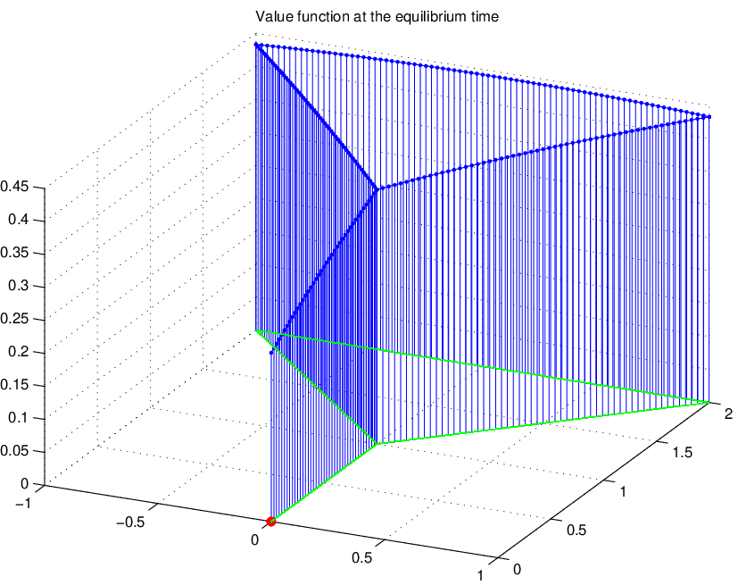
The graph on the right of Figure 1 shows the convergence of the approximated mean field time T2T_{2}, computed by Algorithm 1 with space step h=2.50⋅10−2h=2.50\cdot 10^{-2}. On the horizontal axis are the iterations of the fixed point, while on vertical axis the corresponding approximated mean field time T2T_{2}. In Fig.2, we show the initial mass distribution (left), equilibrium mass distribution (center) and the corresponding value function (right).

hh Eh​(T2)E_{h}(T_{2}) T2T_{2} iterations
1.00⋅10−11.00\cdot 10^{-1} 8.27⋅10−48.27\cdot 10^{-4} 5.687 6
5.00⋅10−25.00\cdot 10^{-2} 1.34⋅10−31.34\cdot 10^{-3} 5.6395.639 7
2.50⋅10−22.50\cdot 10^{-2} 9.04⋅10−49.04\cdot 10^{-4} 5.6175.617 8
1.25⋅10−21.25\cdot 10^{-2} 5.02⋅10−45.02\cdot 10^{-4} 5.6225.622 6
Table 1: Space steps (first column), Eh​(T2)E_{h}(T_{2}) defined in (5.9) (second column), approximated mean field T2T_{2} (third column), number of fixed point iterations (last column)
Refer to captionRefer to captionRefer to caption
Figure 2: Test 1: Initial mass distribution (left), distribution at the equilibrium time (center), value function (right)

5.2 Example 2: A more general graph

We consider a more general graph with 17 vertexes and 22 edges, see Fig.3.

Refer to captionRefer to caption
Figure 3: Left: Graph configuration. Right: approximated mean field time T2T_{2} vs. fixed point iterations, computed by Algorithm 1

The initial mass distribution is given by

m0​(x)=g⁡(x)∫Γg⁡(y)​𝑑y,g⁡(x)=max⁡(0.5−|x−p1|2,0)+max⁡(0.5−|x−p2|2,0)x∈Γ,m_{0}(x)=\frac{g(x)}{\int_{\Gamma}g(y)dy},\quad g(x)=\max(0.5-|x-p_{1}|^{2},0)+\max(0.5-|x-p_{2}|^{2},0)\quad x\in\Gamma,

with p1=(1,3/2)p_{1}=(1,3/2) and p2=(−3/2,3)p_{2}=(-3/2,3). It describes the distribution of two populations, one concentrated around the point p1p_{1}, the other one around p2p_{2}.
The scheduled time is t0=0.5t_{0}=0.5, the maximum waiting time is Tm​a​x=25T_{max}=25, the cost function

c⁡(s)=0.1​max⁡(s−t0,0)+0.1​max⁡(T−s,0)c(s)=0.1\max(s-t_{0},0)+0.1\max(T-s,0)

and the expected percentage of arrival players is θ=0.7\theta=0.7. The Algorithm 1 is run with h=0.05h=0.05, Δ​t=h24\Delta t=\frac{h^{2}}{4} and τ=0.05\tau=0.05. We get T=23.99T=23.99 with error Eh​(T)=2.35⋅10−2E_{h}(T)=2.35\cdot 10^{-2}. The graph on the right of Figure 3 shows the convergence of the approximated mean field time T2T_{2} computed by Algorithm 1: on the horizontal axis is the number of iterations of the fixed point algorithm, whereas on the vertical axis the corresponding mean field time.
Figure 4 shows the mass evolution at different times. It can be observed that at the initial time the diffusion spreads the population in all the directions on the graph, later the cost (2.2) favors the population closer to v0v_{0} to reach the exit before of the population farther away.

Refer to captionRefer to captionRefer to captionRefer to captionRefer to captionRefer to caption
Figure 4: Test 2: Mass distribution at time: t=0,0.025,1.25,5,10,T=24t=0,0.025,1.25,5,10,T=24

6 Appendix

Proof of Prop. 3.2  For the sake of simplicity, KK will denote a constant independent of μ0\mu_{0} and ww and it may change from line to line. Invoking [18, Theorem 5.4] (see also: [10, Theorem 3.2], [13, Theorem 3.6] or [19, Theorem 5.8]) we obtain that there exists a unique classical solution μ\mu to problem (3.6) which fulfills the estimate

|μ|∞≤K​|μ0/w⁡(⋅,0)|∞.|\mu|_{\infty}\leq K|\mu_{0}/w(\cdot,0)|_{\infty}. (6.1)

For e~:=π0​([l0/4,3​l0/4])\tilde{e}:=\pi_{0}([l_{0}/4,3l_{0}/4]), we claim that μ\mu belongs to C(2+α,1+α/2)​(e~×[0,Tm​a​x])C^{(2+\alpha,1+\alpha/2)}(\tilde{e}\times[0,T_{max}]) with

|μ|e~×[0,Tm​a​x](2+α,1+α/2)≤K​|μ0/w⁡(⋅,0)|Γ(2+α).|\mu|^{(2+\alpha,1+\alpha/2)}_{\tilde{e}\times[0,T_{max}]}\leq K|\mu_{0}/w(\cdot,0)|^{(2+\alpha)}_{\Gamma}. (6.2)

In order to prove this estimate, we introduce two families of functions {μ~0,n}n\{\tilde{\mu}_{0,n}\}_{n} and {μ~1,n}n\{\tilde{\mu}_{1,n}\}_{n} such that

μ~0,n,μ~1,n∈C1​([0,Tm​a​x]),|μ~0,n|∞+|​μ~1,n−μ⁡(v1,⋅)|∞→0as ​n→+∞,μ~0,n(0)=0,μ~0,n′(0)=D2(μ0​(⋅)w⁡(⋅,0))(v0),μ~1,n(0)=μ0​(v1)w⁡(v1,0),μ~1,n′(0)=D2(μ0​(⋅)w⁡(⋅,0))(v1),\begin{array}[]{c}\tilde{\mu}_{0,n},\tilde{\mu}_{1,n}\in C^{1}([0,T_{max}]),\qquad|\tilde{\mu}_{0,n}|_{\infty}+|\tilde{\mu}_{1,n}-\mu(v_{1},\cdot)|_{\infty}\to 0\quad\textrm{as }n\to+\infty,\\ \tilde{\mu}_{0,n}(0)=0,\qquad\tilde{\mu}_{0,n}^{\prime}(0)=D^{2}\left(\frac{\mu_{0}(\cdot)}{w(\cdot,0)}\right)(v_{0}),\\ \tilde{\mu}_{1,n}(0)=\frac{\mu_{0}(v_{1})}{w(v_{1},0)},\qquad\tilde{\mu}_{1,n}^{\prime}(0)=D^{2}\left(\frac{\mu_{0}(\cdot)}{w(\cdot,0)}\right)(v_{1}),\\ \end{array}

By standard regularity theory for parabolic equations on domains in Euclidean spaces, the problem

{∂tμn−∂x2μn=0(x,s)∈(0,l0)×(0,Tm​a​x)μn​(0,s)=μ~0,n​(s),μn​(l0,s)=μ~1,n​(s)s∈[0,Tm​a​x]μn​(x,0)=μ0​(x)w⁡(x,0)x∈(0,l0)\displaystyle\left\{\begin{array}[]{ll}\partial_{t}\mu_{n}-\partial^{2}_{x}\mu_{n}=0&(x,s)\in(0,l_{0})\times(0,T_{max})\\[6.0pt] \mu_{n}(0,s)=\tilde{\mu}_{0,n}(s),\quad\mu_{n}(l_{0},s)=\tilde{\mu}_{1,n}(s)&s\in[0,T_{max}]\\[6.0pt] \mu_{n}(x,0)=\frac{\mu_{0}(x)}{w(x,0)}&x\in(0,l_{0})\end{array}\right.

admits a unique classical solution μn\mu_{n} which belongs to C(2+α,1+α/2)​((0,l0)×(0,Tm​a​x))C^{(2+\alpha,1+\alpha/2)}((0,l_{0})\times(0,T_{max})) for some α\alpha depending only on the features of the equation. By [16, Theorem IV.10.1], we deduce the following estimate in the domain (l0/4,3​l0/4)×(0,Tm​a​x)(l_{0}/4,3l_{0}/4)\times(0,T_{max})

|μn|(l0/4,3​l0/4)×(0,Tm​a​x)(2+α,1+α/2)≤K⁡(|μ0/w⁡(⋅,0)|e0(2+α)+|​μn|∞).|\mu_{n}|^{(2+\alpha,1+\alpha/2)}_{(l_{0}/4,3l_{0}/4)\times(0,T_{max})}\leq K\left(|\mu_{0}/w(\cdot,0)|^{(2+\alpha)}_{e_{0}}+|\mu_{n}|_{\infty}\right).

By Ascoli theorem, as n→+∞n\to+\infty, (eventually, passing to a subsequence), the function μn\mu_{n} converges uniformly to some function vv and the same happens for ∂tμn\partial_{t}\mu_{n}, ∂xμn\partial_{x}\mu_{n} and ∂x2μn\partial_{x}^{2}\mu_{n} with the corresponding derivatives of vv. By the stability result we get v=μv=\mu. Moreover, passing to the limit in the last estimate, we obtain

|μ|(l0/4,3​l0/4)×(0,Tm​a​x)(2+α,1+α/2)≤K⁡(|μ0/w⁡(⋅,0)|e0(2+α)+|​μ|∞)|\mu|^{(2+\alpha,1+\alpha/2)}_{(l_{0}/4,3l_{0}/4)\times(0,T_{max})}\leq K\left(|\mu_{0}/w(\cdot,0)|^{(2+\alpha)}_{e_{0}}+|\mu|_{\infty}\right)

and, taking into account estimate (6.1) and the definition of the sub-edge e~\tilde{e}, we accomplish the proof of claim (6.2).

We observe that the function μ|e0,1/2×(0,Tm​a​x)\mu_{|e_{0,1/2}\times(0,T_{max})} is the unique classical solution to problem

{∂tμ¯−∂x2μ¯=0(x,s)∈e0,1/2×(0,Tm​a​x)μ¯​(v0,s)=0,μ¯​(v1/2′,s)=μ⁡(v1/2′,s)s∈[0,Tm​a​x]μ¯​(x,0)=μ0​(x)w⁡(x,0)x∈e0,1/2\displaystyle\left\{\begin{array}[]{ll}\partial_{t}\bar{\mu}-\partial^{2}_{x}\bar{\mu}=0&(x,s)\in e_{0,1/2}\times(0,T_{max})\\[6.0pt] \bar{\mu}(v_{0},s)=0,\quad\bar{\mu}(v^{\prime}_{1/2},s)=\mu(v^{\prime}_{1/2},s)&s\in[0,T_{max}]\\[6.0pt] \bar{\mu}(x,0)=\frac{\mu_{0}(x)}{w(x,0)}&x\in e_{0,1/2}\end{array}\right.

which is a standard initial-boundary value problem on an Euclidean domain. Invoking [16, Theorem IV.9.1], we infer that, for every q≥1q\geq 1, μ\mu belongs to Wq,e0,1/2×[0,Tm​a​x]2,1W^{2,1}_{q,e_{0,1/2}\times[0,T_{max}]} with

|μ|q,e0,1/2×[0,Tm​a​x]2,1≤K⁡(|μ0/w⁡(⋅,0)|e0,1/2(2)+|​μ​(v1/2′,⋅)|(0,Tm​a​x)(1)).|\mu|^{2,1}_{q,e_{0,1/2}\times[0,T_{max}]}\leq K\left(|\mu_{0}/w(\cdot,0)|^{(2)}_{e_{0,1/2}}+|\mu(v^{\prime}_{1/2},\cdot)|^{(1)}_{(0,T_{max})}\right).

Owing to (6.2), estimate (3.7) is achieved. □\Box

Proof of Prop. 3.3  We shall improve some arguments of the proof of Proposition 3.2 taking advantage of the stronger compatibility condition given by (3.8). Here, the constant KK is independent of μ0\mu_{0} and ww and it may change from line to line.

We consider the family of functions {μ~1,n}n\{\tilde{\mu}_{1,n}\}_{n} introduced in the proof of Proposition 3.2. By standard regularity theory for parabolic equations on domains in Euclidean spaces, the problem

{∂tμn−∂x2μn=0(x,s)∈(0,l0)×(0,Tm​a​x)μn​(0,s)=0,μn​(l0,s)=μ~1,n​(s)s∈[0,Tm​a​x]μn​(x,0)=μ0​(x)w⁡(x,0)x∈(0,l0)\displaystyle\left\{\begin{array}[]{ll}\partial_{t}\mu_{n}-\partial^{2}_{x}\mu_{n}=0&(x,s)\in(0,l_{0})\times(0,T_{max})\\[6.0pt] \mu_{n}(0,s)=0,\quad\mu_{n}(l_{0},s)=\tilde{\mu}_{1,n}(s)&s\in[0,T_{max}]\\[6.0pt] \mu_{n}(x,0)=\frac{\mu_{0}(x)}{w(x,0)}&x\in(0,l_{0})\end{array}\right.

admits a unique classical solution μn\mu_{n} which belongs to C(2+α,1+α/2)​((0,l0)×(0,Tm​a​x))C^{(2+\alpha,1+\alpha/2)}((0,l_{0})\times(0,T_{max})) for some α\alpha depending only on the features of the equation. By [16, Theorem IV.10.1], we deduce the following estimate in the domain (0,l0/2)×(0,Tm​a​x)(0,l_{0}/2)\times(0,T_{max})

|μn|[0,l0/2]×[0,Tm​a​x](2+α,1+α/2)≤K⁡(|μ0/w⁡(⋅,0)|[0,l0](2+α)+|​μn|∞).|\mu_{n}|^{(2+\alpha,1+\alpha/2)}_{[0,l_{0}/2]\times[0,T_{max}]}\leq K\left(|\mu_{0}/w(\cdot,0)|^{(2+\alpha)}_{[0,l_{0}]}+|\mu_{n}|_{\infty}\right). (6.3)

By Ascoli theorem, as n→+∞n\to+\infty, (eventually, passing to a subsequence), the function μn\mu_{n} converges to some function vv uniformly and the same happens for ∂tμn\partial_{t}\mu_{n}, ∂xμn\partial_{x}\mu_{n} and ∂x2μn\partial_{x}^{2}\mu_{n} with the corresponding derivatives of vv. By the stability result we get v=μv=\mu. Moreover, passing to the limit in the estimate (6.3), we obtain

|μ|[0,l0/2]×[0,Tm​a​x](2+α,1+α/2)≤K⁡(|μ0/w⁡(⋅,0)|[0,l0](2+α)+|​μ|∞).|\mu|^{(2+\alpha,1+\alpha/2)}_{[0,l_{0}/2]\times[0,T_{max}]}\leq K\left(|\mu_{0}/w(\cdot,0)|^{(2+\alpha)}_{[0,l_{0}]}+|\mu|_{\infty}\right).

Finally, taking into account estimate (6.1), we accomplish the proof.

The second part of the statement is a consequence of [2]; actually, in this case, the compatibility conditions are ensured by (3.10). Invoking [2], we obtain

|μ|Γ×[0,Tm​a​x](2+α,1+α/2)≤K0​|μ0/w⁡(⋅,0)|Γ(2+α)|\mu|^{(2+\alpha,1+\alpha/2)}_{\Gamma\times[0,T_{max}]}\leq K_{0}|\mu_{0}/w(\cdot,0)|^{(2+\alpha)}_{\Gamma}

where K0K_{0} is the same constant as in Proposition 3.1. □\Box

Remark 6.1

As one can easily check, in the proof of previous Proposition 3.3, hypothesis (3.8) is needed only for guaranteeing the compatibility condition in v0v_{0}. As a matter of fact, it can be replaced by: ∂x2(μ0​(⋅)/w⁡(⋅,0))​(v0)=0\partial_{x}^{2}(\mu_{0}(\cdot)/w(\cdot,0))(v_{0})=0.

Acknowledgment.The authors wish to thank Adriano Festa for his help in the algorithm for programming the graph structure

References

  • [1] Y. Achdou. Finite difference methods for mean field games. In Hamilton-Jacobi Equations: Approximations, Numerical Analysis and Applications, volume 2074, Lecture Notes in Math., Springer, Berlin, 2013.
  • [2] J. von Below, Classical solvability of linear parabolic equations on networks. J. Differential Equations 72 (1988), no. 2, 316–337.
  • [3] J. von Below and S. Nicaise, Dynamical interface transition in ramified media with diffusion. Comm. Partial Differential Equations 21 (1996), no. 1-2, 255–279.
  • [4] M.Burger, M. Di Francesco, P.Markowich, M.-T. Wolfram, Mean field games with linear mobilities in pedestrian dynamics, arXiv: 1304.5201
  • [5] F. Camilli, C. Marchi and D.Schieborn, The vanishing viscosity limit for Hamilton-Jacobi equation on networks, J. Differential Equations 254 (2013), no. 10, 4122–4143.
  • [6] P. Cardaliaguet, Notes on Mean Field Games: from P.-L. Lions’ lectures at Collège de France, Lecture Notes given at Tor Vergata, 2010.
  • [7] G.M. Coclite and M. Garavello, Vanishing viscosity for traffic on networks, SIAM J. Math. Anal 42 (2010), 1761–1783.
  • [8] C. Dogbé, Modeling crowd dynamics by the mean-field limit approach. Math. Comput. Modelling 52 (2010), no. 9-10, 1506-1520.
  • [9] M. Freidlin and S.J. Sheu, Diffusion processes on graphs: stochastic differential equations, large deviation principle. Probab. Theory Related Fields 116 (2000), no. 2, 181–220.
  • [10] M. Freidlin and A. Wentzell, Diffusion processes on graphs and the averaging principle. Ann. Probab. 21 (1993), no. 4, 2215–2245.
  • [11] M. Garavello, B. Piccoli, Traffic Flow on Networks. AIMS Series on Applied Mathematics, Vol. 1, American Institute of Mathematical Sciences, 2006.
  • [12] D. Gomes and J. Saude, Mean field games - A brief survey. Dyn.Games App., to appear.
  • [13] M. Kramar Fijavz, D. Mugnolo and E. Sikolya, Variational and semigroup methods for waves and diffusion in networks. Appl. Math. Optim. 55 (2007), no. 2, 219–240.
  • [14] O. Guéant, J-M. Lasry and P-L. Lions. Mean field games and applications. In “Paris- Princeton Lectures on Mathematical Finance 2010”, volume 2003, Lecture Notes in Math., Springer, Berlin, 2011.
  • [15] O. Guéant, Mean field games equations with quadratic Hamiltonian: a specific approach, M3AS Math. Models Methods Appl. Sci. 22 (2012), no.9, 1250022.
  • [16] O.A. Ladyzenskaja, V.A. Solonnikov, and N.N. Uralceva, Linear and Quasi-linear Equations of Parabolic Type. American Mathematical Society, Providence, R.I., 1968.
  • [17] J-M. Lasry and P-L. Lions. Mean field games. Jpn. J. Math., 2 (2007), no. 1, 229–260.
  • [18] D. Mugnolo, Gaussian estimates for a heat equation on a network, Netw. Het. Media 2 (2007), 55–79.
  • [19] D. Mugnolo and S. Romanelli, Dynamic and generalized Wentzell node conditions for network equations, Math. Methods Appl. Sci. 30 (2007), 681–706.
  • [20] B. Piccoli and A. Tosin, Time-evolving measures and macroscopic modeling of pedestrian flow. Arch. Ration. Mech. Anal. 199 (2011), no. 3, 707-738.