Probing atomic environments in alloys by electron spectroscopy
Abstract
In alloys exhibiting substitutional disorder, the variety of atomic environments manifests itself as a ‘disorder broadening’ in their core level binding energy spectra. Disorder broadening can be measured experimentally, and in principle can be used to deduce information about specific atomic environments within a sample. However, progress in this endeavor is hampered by the lack of a model for this phenomenon which can treat complex systems. In this work we describe such a model. The model is used to elucidate the relationship between charge transfer, atomic environment, and disorder broadening in complex systems, with a focus on the problem of characterizing the interface quality of CuNi multilayers. We also validate the model against the results of ab initio electronic structure calculations. Several counterintuitive aspects of the disorder broadening phenomenon are uncovered, an understanding of which is essential for the correct interpretation of experimental results. For instance, it is shown that systems with inhomogeneous concentration profiles can exhibit disorder broadenings significantly larger than random alloys. Furthermore in some systems a ‘disorder narrowing’ is even possible.
pacs
71.23.-k, 79.60.Ht, 79.60.JvI Introduction
An atom’s core level binding energies depend on its chemical species. This fact has been exploited for decades in order to determine the proportion of different species within a given sample via core level spectroscopy - which provides the distribution of core electron binding energies within a sample. An atom’s binding energies also depend on its environment, i.e., the species of its surrounding atoms. For instance, in a Cu metal all atoms have the same environment, and hence the binding energies for a given Cu core level type, e.g. 2p3/2, will be the same for all atoms. By contrast, in a CuPd alloy exhibiting substitutional disorder the Cu atoms exhibit a variety of environments, and hence also a variety of 2p3/2 binding energies. Such a dispersion in the binding energies has been observed in many alloy systems [1, 2, 3, 4, 5, 6, 7, 8], and in theory can be used to deduce information about specific environments within a sample, including the concentration profile on the atomic scale. The viability of achieving this via high kinetic energy photoelectron spectroscopy (HIKE) has recently been demonstrated [7, 8]. This is promising because HIKE, unlike other widely-used techniques, is both bulk-sensitive and non-destructive. Such environment-resolved spectroscopy would prove useful to the many research areas involving alloys in which segregation plays a crucial role, e.g. metal embrittlement [9, 10, 11, 12, 13, 14], and nanocatalyst design [15, 16]. However, success in this endeavor hinges upon a solid understanding of the relationship between an atom’s environment, its electronic structure, and its core level binding energies in alloys.
The central quantity with regards to environment-resolved spectroscopy in alloys is the (alloy-metal) core level shift (CLS), which for a core level bound to an site is defined as
| (1) |
where is the binding energy of the core level, and is the binding energy of the core level belonging to the type under consideration in a pure metal. Note that this is a site-dependent quantity; one must determine for all sites in the system under consideration in order to determine the CLS distribution. This is problematic for systems exhibiting substitutional disorder on account of their lack of periodicity - which is a prerequisite for treatment within the conventional theoretical framework exploited by most ab initio methods. One way around this problem is to approximate the system under consideration as periodic, but with a large unit cell, i.e., a supercell. In this supercell approximation one determines for all sites, and hopes that the range of environments exhibited by these sites is representative of the ‘true’ (non-periodic) system, and hence will result in an accurate representation of the true CLS distribution.
Random alloys - the archetype of disordered alloys in which there are no correlations between the species of sites - are the most tractable system exhibiting substitutional disorder to treat theoretically, and have been the focus of both experimental [1, 2, 3, 4, 5, 6, 17] and theoretical [18, 1, 2, 19, 20, 21, 22, 23, 6, 17] attempts to understand the distribution of CLSs in alloys. In this context the dispersion of CLSs is known as ‘disorder broadening’ on account of the increased width of, for example, the Cu CLS distribution for a CuPd random alloy relative to that for a Cu metal. Sophisticated ab initio models utilizing the supercell approximation have provided insight into disorder broadening in these systems [22, 23, 6, 17]. However, most systems of practical interest cannot be idealized as random alloys, and unfortunately the complexity of these systems is such that a description of their disorder broadenings using ab initio models is intractable within the supercell approximation.
Accurate methods do exist which do not resort to the supercell approximation. Ab initio methods rooted in the coherent potential approximation (CPA)[24, 25, 26] have been shown to provide excellent agreement with experiment [27, 28, 29, 30, 17]. Furthermore, they can treat complex systems [30, 7, 17]. However, CPA-based approaches cannot provide detailed information regarding the disorder broadening in complex systems - nor even random alloys. While phenomenological models have been developed which can provide such information [18, 1, 2, 19, 21], their accuracy has been questioned [31, 32, 33]. One criticism is that these models do not take into account ‘final state effects’ associated with changes in the valence electron density after photoemission. It has even been claimed that the complexity of the relationship between CLSs and environment in alloys precludes an accurate alternative to ab initio methods [33].
Here we present an accurate phenomenological model for CLSs in alloys which relates - including the final state contribution - to the environment of site . The model, like previous approaches, is charge-transfer based, and provides a simple framework for rationalizing the disorder broadening phenomenon. The layout of this work is as follows. In Sec. II we review the theory which underpins the model, and derive expressions for CLSs which apply to a wide range of alloy systems. We then apply the model to the problem of characterizing the interface quality of metallic multilayers. This problem has received significant attention on account of its importance to nanotechnology [34, 7, 8, 17], and can be restated as follows: what is the degree of ‘interface roughening’ in a given sample? Fig. 1(a) provides an illustration of the multilayer system [Ni5/Cu5] with various - where the square brackets signify that the system at consists of a 10 monolayer stack Ni5/Cu5 repeated throughout all space. In this regard, Sec. III contains details of our calculations, and our results are presented in Sec. IV. Finally, in Sec. V we summarize our main findings, and discuss the limitations of the model, and intentions for future work. Note that throughout this work we use Hartree atomic units unless otherwise stated. To transform energies within Hartree atomic units to eV the former quantity should be multiplied by a factor 27.2114.

II Theory
Our model is based upon the charge-excess functional model [35] within the non-random approximation [36, 21] (NRA-CEFM). After briefly reviewing the NRA-CEFM in Sec. II.1, in Sec. II.2 we use it to derive a relation between and the environment of site . In the subsequent subsections this relation is itself used to derive expressions for the mean and full width at half maximum (FWHM) of various CLS distributions. While our expression for presented in Sec. II.2 is valid for any alloy - subject to the assumptions which underpin the NRA-CEFM - our expressions for means and FWHMs apply only to the class of alloys which can be described as having a concentration profile which varies along one direction from monolayer to monolayer. To elaborate, for an alloy belonging to this class, the quantities for all and describe the concentration profile, where denotes the concentration of sites within monolayer , and we are assuming that the species of sites belonging to a given monolayer are assigned randomly in the appropriate concentrations. Note that this class includes random alloys, for which for all , where denotes the global concentration of species . Furthermore, note that we use the following convention for labeling the monolayers: monolayer is the th monolayer in the direction in which the concentrations of each species are varying.
II.1 The charge-excess functional model in the non-random approximation
The charge-excess functional model (CEFM) [35] has been shown to provide an accurate description of the charge distribution in disordered alloys [35, 36, 37]. It has also been shown to provide an accurate description of energy differences between alloy configurations with the same composition [37] - where by composition we mean a specification of the underlying lattice and the quantities for all . In the CEFM the alloy energy is postulated to take the form
| (2) |
where
| (3) |
is the Madelung energy, is the Madelung potential of site , is the net charge on site , is the strength of the ‘local interactions’ within site which act to keep the charge of site at its ‘bare’ value , and is a constant. For all sites, and take the same values and respectively. Minimizing subject to the constraint of charge neutrality leads to the following expression [35]:
| (4) |
where
| (5) |
and is a Lagrange multiplier added to enforce charge neutrality. Eqn. (4) describes the Q-V relations, which are borne out in ab initio calculations to a high degree of accuracy [38, 39, 40, 37]. This partly explains the success of the CEFM.
Eqn. (2) can be derived within the class of generalized coherent potential approximations (GCPAs) described by Bruno et al. [37], with the additional - essentially exact [37] - assumption that charge transfer due to Madelung interactions 11 1 In this work the term ‘Madelung interactions’ is used as a synonym for ‘inter-site Coulomb interactions’. is small. Here we consider the CEFM within this framework, in which case is equivalent to the charge of an site embedded in the GCPA effective medium for the system under consideration, given the constraint that the site’s Madelung potential is 0. In other words, is the charge of an site embedded in the effective medium if the Madelung interactions are ‘switched off’. Furthermore, is the linear response coefficient relating the Madelung potential of the site to its perturbation from , and is the energy of the alloy if the Madelung interactions between sites are switched off - which can be expressed as
| (6) |
where is the energy of an site embedded in the effective medium if Madelung interactions are switched off, and is the total number of sites in the system. Conventional CPA calculations do not take into account Madelung interactions, and hence for GCPA theories based upon CPA effective media is simply the charge of an site obtained from a conventional CPA calculation, and is the corresponding energy. Calculations reveal that GCPA effective media are numerically indistinguishable [37] for all alloys with the same composition. Hence the same applies for the quantities , and : these quantities are transferable between such systems.
The complexity of the CEFM is significantly reduced if one makes the assumption that takes the same value for all species [36, 41, 21]. This assumption is known as the non-random approximation (NRA), and we use it throughout this work. The non-random approximation is borne out calculations utilizing the single-site locally self-consistent Green’s function method [40] - a GCPA method. In the NRA-CEFM for an site obeys [21]
| (7) |
where: is the number of sites in the th nearest neighbor shell of site ;
| (8) |
and the quantities and for all depend only on and the underlying lattice type 22 2 By lattice type we mean, for example, fcc, bcc, sc. Note that two lattices with the same type can have different values of . - where is the Wigner-Seitz radius for the system under consideration - and are tabulated in Ref. 21 for the fcc, bcc and sc lattices. Note that the free parameters and (for all ) can be obtained from ab initio calculations or by other means [21]. Furthermore, the values of for all and characterize the environment of . Therefore Eqn. (7) explicitly relates to the environment of site . Eqn. (7) also allows us to interpret an alloy’s charge distribution in terms of charge transfer between pairs of unlike sites as follows [21]: an site gains a charge from each site in its th nearest neighbor shell, with the site losing the opposite amount. This picture allows us to attribute the following physical significance to the quantity : it is a measure of the electropositivity of species for the given composition.
II.2 Expression for
We will now use the NRA-CEFM to derive an expression for the CLS of site . To do this, we first derive an expression for the total energy in terms of the bare charges of all sites. Eqn. (2) can be rewritten more explicitly as
| (9) |
for the NRA-CEFM, where we have used Eqn. (3). Minimizing this with respect to the site charges, and subject to the constraint of global charge neutrality gives [21]
| (10) |
where denotes the mean value of over all . Substituting the above into Eqn. (9) and simplifying gives
| (11) |
where we have used the fact that
| (12) |
Now, the following expression holds for the charges at the minimum in [21]:
| (13) |
where
| (14) |
denotes the Madelung matrix, and denotes the identity matrix. This becomes
| (15) |
since [36]
| (16) |
Substituting Eqn. (15) into Eqn. (11) gives
| (17) |
which becomes
| (18) |
after separating out the terms containing and noting that is a symmetric matrix [36]. We will use the above equation in a moment.
The binding energy of a core level associated with site is
| (19) |
where denotes the energy of the alloy’s initial state - before photoemission from site , and denotes the energy of the alloy’s final state - after photoemission from site . In the complete screening picture [42] the valence electrons in the final state are assumed to be fully relaxed so to reach their minimum energy configuration. With this in mind, the energy of the final state is simply the energy of the initial state, but with the atomic core within replaced by its photo-ionized analogue. We choose site to belong to species , and denote the ‘species’ corresponding to a photo-ionized site as . Hence is the energy change if site , originally belonging to species , is transformed into species . Eqn. (18) allows us to evaluate the change in due to such a transformation. Noting that the terms on the lower line of Eqn. (18) are unaffected by the transformation (since and for all are composition-dependent, and the composition - which we defined in terms of macroscopic quantities - is unaffected by the transformation), that the transformation is such that , and also that (see Eqn. (6)), we obtain
| (20) |
This can be rearranged to give
| (21) |
which in turn becomes
| (22) |
after using Eqn. (15) and noting that [21]. We emphasize that in the above equation refers to the charge of site before photoemission. Finally, substituting the above equation into Eqn. (1), and relabeling site as site , we obtain the following expression for the CLS associated with site :
| (23) |
where
| (24) |
is composition-dependent.
Eqn. (23) describes a species- and composition-dependent linear mapping between and . Therefore changes in the CLS distribution associated with configuration changes - such as an increase in the interface roughening in a multilayer system - directly reflect changes in the charge distribution. Furthermore the shape of the CLS distribution is the same as that of the charge distribution on account of the linear nature of the mapping between and . We will elaborate on these points later.
II.3 Mean and FWHM of various CLS distributions
Henceforth we consider the mean and FWHM of the CLS distributions for various groups of sites. Note that the FWHM of any random variable is related to its variance by the equation
| (25) |
We will use this fact several times below. We will also use the fact that the mean and FWHM of for any group of sites within a given alloy, as follows from Eqn. (23), are given by
| (26) |
and
| (27) |
respectively, where and denote the mean and variance of the charge distribution for .
II.3.1 Random alloys
Consider the group of all sites within a random alloy. For random alloys [21]
| (28) |
and
| (29) |
where denotes the variance of over all sites in the system, and depends only on and the underlying lattice type, and is tabulated in Ref. 21 for the fcc, bcc and sc lattices. Therefore for random alloys Eqns. (26) and (27) yield
| (30) |
and
| (31) |
where we have defined
| (32) |
and used the fact that [21]
| (33) |
For binary alloys consisting of species and the above equations simplify to
| (34) |
and
| (35) |
for .
II.3.2 Mean for a single monolayer
Henceforth we consider the class of systems described at the beginning of this section in which the species concentrations
can vary from monolayer to monolayer. Let be the set of sites within monolayer . Furthermore, let and denote the mean and FWHM respectively of the CLS distribution for . A similar notation will be used later for other quantities, e.g. and . We will now derive an expression for . Consider a site within . From Eqn. (7), can be expressed as
| (36) |
where denotes the number of sites in the th nearest neighbor shell of which are in monolayer . Taking the mean over all gives
| (37) |
Now, over describes a random variable distributed according to the multinomial distribution. Specifically, is the number of times outcome occurs in trials, given the probability of outcome in a single trial is , where is the total number of sites in the th nearest neighbor shell of any site which also belong to one monolayer which is ‘ monolayers away’ from - with referring to the monolayer which contains site itself. The properties of the multinomial distribution are such that , and hence the above equation becomes
| (38) |
This can be rewritten as
| (39) |
where we have defined
| (40) |
Finally, substituting Eqn. (39) into Eqn. (26) gives
| (41) |
For species in a binary alloy the above simplifies to
| (42) |
The quantities depend on the lattice type, , and the set of lattice planes which constitute the monolayers. They determine the coupling between monolayers with regards to and . It can be shown that for the concentration profile for all , i.e., a random alloy, the above equations become equivalent to those given earlier for random alloys. This is the case since
| (43) |
which can be shown by noting that
| (44) |
and [21]
| (45) |
II.3.3 FWHM for a single monolayer
We will now derive an expression for . Taking the variance of Eqn. (36) over gives
| (46) |
after noting that the random variables and , defined by considering and for , are independent if or . Expanding the variance on the right-hand side gives
| (47) |
where denotes the covariance of random variables and . Because over form a multinomial distribution,
| (48) |
and
| (49) |
Substituting these equations into Eqn. (47) gives
| (50) |
where we have defined
| (51) |
Substituting Eqn. (50) into Eqn. (27) gives
| (52) |
For species in a binary alloy the above equation simplifies significantly:
| (53) |
The quantities determine the coupling between monolayers with regards to and . As was the case for , if for all then the above equations become equivalent to those given earlier for random alloys. This is the case since
| (54) |
which can be shown by appealing to Eqn. (44) as well as the definition of :
| (55) |
II.3.4 Total mean
From the quantities for all , the mean CLS over all sites in the system under consideration can be determined by using the following expression:
| (56) |
where is the weight to be given to monolayer . For the ‘true’ mean, is given by
| (57) |
However, one is often interested in the mean of the CLS distribution observed experimentally, which may differ from the ‘true’ value on account of the fact that the probability of a photoelectron emitted from monolayer escaping the alloy is monolayer-dependent. In this case is given by
| (58) |
Eqn. (56) follows trivially from the following theorem: if is a set of values whose mean is , then the mean of the superset formed by combining the sets for all is
| (59) |
This result can be derived from the definitions of and :
| (60) |
II.3.5 Total FWHM
From the quantities , and and for all , the FWHM in the CLS distribution over all sites can determined using the following expression:
| (61) |
Eqn. (61) can be derived by applying Eqn. (25) to the analogous equation to Eqn. (59) for the variance:
| (62) |
where denotes the variance of , and denotes the variance of . The above equation can itself be derived somewhat similarly to Eqn. (59):
| (63) |
which becomes Eqn. (62) after noting that the final term in the last equality vanishes.
III Computational details
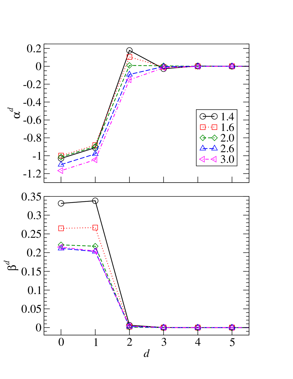
In the next section we apply the expressions of Sec. II.3 to various multilayer systems. All systems we consider have an fcc underlying lattice, and the monolayers are the 001 planes. However, to apply these expressions we first had to determine the monolayer coupling parameters and , which are defined in Eqns. (40) and (51). In Ref. 21, and are tabulated as a function of for the fcc, bcc and sc lattices. Using this information, and after determining the quantities - which depend on the underlying geometry - one can tabulate and as a function of for any fcc, bcc or sc system. For other lattice types, and must be determined as a function of beforehand. A procedure to do this is described in Ref. 21. We determined and for the 001 planes of the fcc lattice at selected . The results are shown in Fig. 2. We considered 1.4, 1.6, 2.0, 2.6 and 3.0, which reflects the range of found in the literature [38, 39, 40, 37, 43, 44, 17]. Note that the coupling between monolayers rapidly tends to zero with .
In addition to the aforementioned ‘analytical’ results, we also performed supercell calculations for each of the systems we considered. In our supercells, each monolayer contained 200 sites, with the species of sites in each monolayer assigned randomly such that the desired species concentrations were obtained as closely as possible. was determined for each site using Eqns. (23) and (7). These where then used to determine , , and in the conventional manner, which allowed us to cross-check our analytical results. For all systems the analytical and supercell results were in excellent agreement, though we choose not to present the supercell means and FWHMs for the sake of brevity and clarity of presentation. In addition to cross-checking, the supercell values of were used to simulate core level spectra for some systems. In this regard we used the following equation:
| (64) |
where denotes the intensity of the spectrum at CLS , is a Lorentzian function with FWHM , and is the lifetime broadening of the core levels under consideration. The above equation does not take into account many features which are present in ‘real’ spectra such as surface core-level shifts, experimental broadening, Doniac-Sunjic asymmetry, and inelastic scattering. However, since our simulated spectra are primarily for illustrative purposes, ignoring these complications is justified. Our supercell calculations served one further purpose. Later we present histograms of, for binary systems, the frequency of sites exhibiting each possible number of nearest neighbors, and for ternary systems, the frequency of sites exhibiting each possible combination of and nearest neighbors. We used our supercells to generate these histograms: for each supercell we counted the number of sites with each possible composition of nearest neighbor shell.
IV Results
IV.1 Isolated embedded thin film:
We first present results for systems consisting of a thin film of species and thickness monolayers embedded in a substrate, i.e., . We examined such systems with various and , where recall that denotes the degree of interface roughening. Following Refs. 34, 17, interface roughening was modeled by convoluting the ‘unroughened’ concentration profile with a discrete Gaussian function [34], where denotes the standard deviation of the function. To elaborate, the concentration profile corresponding to was calculated using the following equation:
| (65) |
for all , where
| (66) |
is the discrete analogue of a Gaussian function with standard deviation , and denotes the unroughened concentration profile.
IV.1.1 General results
The quantities , , and for various systems are presented in Figs. 3 and 4. In calculating these values, we used the set of described in the previous section. Furthermore, we set , , and . Results (in eV) obtained using these parameters can be generalized to any choice of (in bohrs), , (both in units of ) and (in eV) at the corresponding value of by multiplying all means and FWHMs by , and additionally adding to all mean CLSs. We will use this fact in a moment.
Some interesting results are immediately apparent from Figs. 3 and 4. Firstly, as can be seen from both figures, the model results only depend weakly on . This is convenient because the ‘true’ value of for a given system is unclear; values of are very sensitive to the ab initio method used to obtain them. The same is true for the quantities , and presumably also for the quantities and . This is illustrated in Table 1, where the and for the bcc random alloy Cu0.5Zn0.5 obtained using different ab initio methods are compared. In calculating each in the table we took to be the mean of the ab initio Q-V relation gradients and for Cu and Zn. Furthermore, we calculated from the Q-V relation intercepts via (see Eqn. (5)).
| Method | ||
|---|---|---|
| LSMS[38, 39, 43] | 2.5 | 0.16 |
| GCPA[37] | 1.6 | 0.12 |
| LAPW[37] | 3.5 | 0.16 |
Our second observation relates to Fig. 4. One might expect that, at a given composition and parametrization of the model (i.e., choice of the quantities , , and ), the FWHM would be maximized at the random alloy configuration. This configuration corresponds to the largest configurational entropy, and therefore might be expected to exhibit the largest range of environments and hence also the largest FWHM. Moreover, since, as can be seen from Eqn. (35), is maximized when , one might therefore also expect that the corresponding FWHM, which is an upper bound for the FWHM of a random alloy, is also an upper bound for all alloys. However, our results reveal that this is not the case. In each panel of Fig. 4, the random alloy upper bound corresponding to the same model parametrization as we used for our systems is indicated by a dotted line. Note that for some systems is significantly larger than the random alloy upper bound. It is even possible for the upper bound to be exceeded in ‘unroughened’ ultra-thin films - as is evident from the left-most column in Fig. 4. Therefore inhomogeneous concentration profiles can yield larger disorder broadenings than is possible in random alloys - a fact which we provide an explanation for later. A similar observation has been made in our earlier study[20] using the linear charge model[45]: surface segregation was shown to result in a significantly larger disorder broadening relative to the unsegregated random alloy. However in that study surface effects are implicit in the simulated spectra, and hence cannot be discounted as a contributing factor to the very large broadening. By contrast here we have shown that a very large broadening can occur in the absence of surface effects. In the aforementioned study we suggested that segregation could explain the anomalously large disorder broadening observed experimentally by Medicherla et al.[46]. Our results here provide further evidence for this hypothesis.
In contrast to , the monolayer FWHMs seem to be constrained to be below the random alloy upper bound. This can be understood by noting that the sites in monolayer experience a local environment which closely resembles a random alloy, and hence (to a good approximation) cannot exceed the upper bound. Considering only nearest neighbors, each site in monolayer has nearest neighbors in monolayer , in monolayer , and in monolayer . Since within each monolayer we have assigned sites’ species randomly in the required concentrations, it follows that the environment of an site in monolayer is approximately that of a random alloy with concentration
| (67) |


IV.1.2 Comparison with ab initio results
The systems we considered were deliberately chosen to be identical to the fcc systems considered in Ref. 17, in which Olovsson et al. calculated for Ni/CuT/Ni and Co/CuT/Co. The and determined by Olovsson et al. are shown in Fig. 5. Comparing this figure with Fig. 3 we see that the model is in excellent qualitative agreement with those of Olovsson et al. for the Ni/CuT/Ni systems. The agreement is especially good at higher values of . For the Co/CuT/Co systems, the agreement is reasonable. However, it should be borne in mind that the dispersion of CLSs in Co/CuT/Co is very small, and hence any uncertainties implicit in the ab initio method used by Olovsson et al. will be larger relative to the size of the dispersion: Olovsson et al. quote CLSs to a precision of 10meV, which is significant on the scale of the Co/CuT/Co dispersion, but not for the Ni/CuT/Ni dispersion.
The used by Olovsson et al. in their calculations was 2.6 bohrs for both Ni/CuT/Ni and Co/CuT/Co. With this in mind, and recalling the procedure described above for generalizing our model results to different free parameters, we found that , eV and gave excellent agreement with Olovsson et al. for Ni/CuT/Ni. For Co/CuT/Co we found acceptable agreement when , , and eV. These values are similar to analogous quantities obtained from ab initio calculations for other alloys [38, 39, 40, 37, 43, 44, 17]. However, as mentioned earlier, the values of these quantities are sensitive to the ab initio method used to obtain them. Hence an interesting prospect is to use the model to determine their values experimentally.
Olovsson et al. used the from their calculations to simulate core level XPS spectra. However, since their calculations did not provide values for , it was necessary for Olovsson et al. to make some assumptions regarding these quantities. They assumed that was the same for all . Fig. 4 reveals that, in fact, the quantities vary widely within any one system. Hence the assumption made by Olovsson et al. is incorrect. However, it is unclear whether the breakdown of this assumption is important from a practical point of view. While accurate knowledge of the quantities - as well as perhaps higher moments of the CLS distribution for each monolayer - is necessary to reproduce the fine details of the total CLS distribution for the system under consideration, in practice these fine details are ‘smeared out’ in the experimental spectrum due to complications such as lifetime and experimental broadening. Therefore getting some of the fine details wrong in the spectrum before accounting for the aforementioned complications may be inconsequential with regards to accurately reproducing experimental spectra.

It should be noted that Olovsson et al. considered a further system in their study in addition to Ni/CuT/Ni and Co/CuT/Co: Fe/CuT/Fe. We do not perform a thorough comparison between our model calculations and those of Olovsson et al. for Fe/CuT/Fe because the underlying lattice for Fe/CuT/Fe is bcc, while our model calculations are for an fcc underlying lattice. At and , the qualitative nature of the ab initio Fe/CuT/Fe results is similar to that for Ni/CuT/Ni and Co/CuT/Co. In these cases we therefore expect that the model will perform well for Fe/CuT/Fe. However, as pointed out by Olovsson et al., a well-known interface state exists in ordered, but not in disordered Fe/CuT/Fe systems, which causes ‘anomalous’ results for . It would be interesting to see whether model calculations utilizing a bcc lattice can reproduce this.
IV.2 Periodic NiCu multilayers: [NiT/CuU]
In the previous subsection we considered an isolated thin film embedded in an infinite substrate. This was done primarily to allow comparison with analogous ab initio results. However, experimental studies have focused on periodic multilayer systems. We now consider such systems; specifically, those comprised of Ni and Cu in which the repeating unit consists of monolayers of Ni adjacent to monolayers of Cu, i.e., [NiT/CuU]. We considered various , and . As above, we used Eqn. (65) to obtain the concentration profile for a given . With regards to the parametrization of the model, we used the ‘best-fit parametrization’ described above for the Ni/CuT/Ni systems, i.e., , eV, and .
The and for various [NiT/CuU] systems as a function of are presented in Fig. 6; we show the ‘trajectory’ of the pair as is varied from 0 to . Note that at intermixing between the Ni and Cu regions is absolute, and [NiT/CuU] becomes a random alloy with . As is evident from Fig. 6, as increases, becomes more negative, and increases initially, before decreasing and finally settling on the random alloy value. The exception is [Ni1/Cu5], for which monotonically decreases with , i.e., the system exhibits a ‘disorder narrowing’. We will now explain these trends.

IV.2.1 Rationalization of spectral changes
A pleasing feature of the model is that it provides a simple means of rationalizing changes in CLS spectra due to configurational changes. Consider Eqn. (7). An insightful approximation is to ignore the dependence of on the environment of site beyond its nearest neighbor shell, in which case for Cu in NiCu systems the number of Ni nearest neighbors of site wholly determines 33 3 A more accurate approach would be to apply ‘mean-field boundary conditions’ beyond the nearest neighbor shell, i.e., assume that for , where recall that denotes the number of sites in any site’s th nearest neighbor shell, and denotes the global concentration of Ni. This would lead to better agreement between the histograms and model spectra in Fig. 1)(b). However, we do not do this here for the sake of simplicity.. Specifically, is linear in :
| (68) |
The same then applies to (from Eqn. (23)):
| (69) |
Using the above expression the Cu spectrum can be decomposed into, or constructed from, components associated with Cu atoms with each value of , which allows us to equate changes in the Cu spectrum to changes in the system’s ‘ histogram’ for Cu.
This is done in Fig. 1(b) for [Ni5/Cu5], where we have used eV in the simulated spectra. At Cu sites exhibit only two possible environments, or 4, with the former corresponding to the 3 ‘central’ monolayers of the 5 monolayer Cu stack and the latter corresponding to the 2 ‘edge’ monolayers. On the whole Cu sites exhibit higher values of as Cu diffuses into the Ni region, leading to a shift in the spectrum to low binding energies as increases. The width of the spectrum increases as the histogram becomes ‘flat’ near , and then narrows again as and the histogram tends to that corresponding to the random alloy Ni0.5Cu0.5. Note that, as we found earlier to be the case for the systems, the disorder broadening is not maximized at the random alloy configuration. An explanation for this is as follows. The histograms for random alloys - substitutionally disordered systems with homogeneous concentration profiles - are binomial distributions. For inhomogeneous concentration profiles, such as those for [Ni5/Cu5] at , the histograms are not constrained to be binomial distributions - they are free to be ‘flatter’. Therefore systems with inhomogeneous concentration profiles can exhibit significantly larger disorder broadenings than random alloys - as is borne out in Figs. 1(b), 4 and 6.
As another example, consider [Ni1/Cu5], which we earlier pointed out exhibits a disorder narrowing. Fig. 7 is analogous to Fig. 1, but for [Ni1/Cu5]. Again, we used eV in the simulated spectrum. At the Cu sites in the 2 edge monolayers of a 5 monolayer Cu stack have , while the Cu sites in the 3 central monolayers have . This is in fact exactly the same situation as for [Ni5/Cu5]. As is increased the Cu sites begin to exhibit other values of ; some Cu sites begin to ‘occupy’ the ‘states’ which were unoccupied at . The same also occurs in [Ni5/Cu5]. However, comparing Figs. 1 and 7 it can be seen that there is a significant occupation of the states in [Ni5/Cu5] which does not occur in [Ni1/Cu5] on account of the lack of Ni. Hence in [Ni1/Cu5], loosely speaking, the Cu sites spill from their and states into only the states as is increased, which results in a narrowing of the spectrum in this system.

IV.2.2 Comparison with experimental results
Experimental Cu spectra for [Ni5/Cu5] and [Ni5/Cu2] at various temperatures were obtained in Refs. 7, 8. However, the spectra were found to depend strongly on the material used to cap the sample, and also on the photon energy used [8]. This is due to the finite escape depth of the photoelectrons, which leads to Cu sites near the surface being ‘over-represented’ in the Cu spectra. Our model results do not account for such surface effects; they pertain to the deep bulk. Hence a quantitative comparison between our model results and most of the experimental spectra is meaningless. The possible exception is the spectra for [Ni5/Cu5] in Ref. 8 taken using a photon energy of 6030eV - which corresponds to a relatively low surface sensitivity. These spectra reveal a shift of eV in [Ni5/Cu5] upon heating over the temperature range corresponding to the transition from to . This is in excellent agreement with our results: as can be seen from Fig. 6, from to the model predicts a shift in the Cu CLS of eV for [Ni5/Cu5]. In the future it would be interesting to perform model calculations which take into account surface effects, and which therefore can be compared directly with the results of Refs. 7, 8.
IV.3 Ternary systems
Finally, we consider ternary multilayer systems - consisting of three species , and . Recall that the CLS distribution reflects the charge distribution (Eqn. (23)), which itself is determined by charge transfer between and non- sites (Eqn. (7)). In binary systems Eqn. (7) gives
| (70) |
where we have used the fact that . Without loss of generality let , which corresponds to choosing species to be the most electronegative of and . From the above equations it can be seen that the electropositivity difference between species and acts only as a scale factor for the and charge distributions; altering has no effect on the qualitative nature of the and charge distributions. Ternary systems are more complicated. The analogous equation to the above for species in a ternary system is
| (71) |
Note that altering affects the charge transfer between site and local sites, while leaving the transfer with local sites unaffected; and conversely if is altered. Hence altering or non-trivially alters the charge distribution. In this sense ternary systems are extremely rich. An exhaustive survey of what can be expected from such systems is beyond the scope of this work. We instead limit ourselves to two ternary systems which we have found to exhibit somewhat counterintuitive behaviors. Furthermore, we limit our discussion to the qualitative aspects of these systems, with a focus on understanding these behaviors. For both systems species is the focus of our attention.
IV.3.1 Periodic ternary multilayer:
The first ternary system we consider is . Again, we use Eqn. (65) to model the interface roughening; Fig. 8(a) gives a schematic illustration of the system at the we considered. For our calculations we set the electropositivities of each species to be , and : the electropositivity of species is exactly halfway between those of species and , with species being the most electronegative and species being the most electropositive. With regards to the other model parameters we set , , , , and . Fig. 8(c) shows the simulated spectra at each . As is evident from the figure, the mean of the CLS distribution is independent of . Hence here one cannot use the mean to characterize in this system - one must use the FWHM. This stems from the choice of species electropositivities. Charge transfer from to and to is always equal and opposite on account of the electropositivity of being exactly between that of and . This, in conjunction with the symmetry of the system, always yields a global mean charge of 0 regardless of , and hence, from Eqn. (23), a -independent mean CLS. Another interesting feature of this system is that the and spectra are ostensibly indistinguishable. Hence unambiguously determining in this system from the spectrum alone is difficult.
The method described earlier for rationalizing spectral changes in binary systems can be extended to ternary systems. The analogous equation to Eqn. (69) for species in a ternary system is
| (72) |
Note that here depends on the environment of through the pair ; there is a mapping from to . Hence the spectrum reflects the ‘ histogram’ of species . This is illustrated in Fig. 8(b-c). Fig. 8(b) illustrates the frequency of sites with each (i.e., the histogram for species ), as well as the CLS for each - contours of constant CLS in ‘-space’ are drawn. If an environment is exhibited by a high frequency of sites, then there is a spike in the CLS spectrum at the corresponding CLS. This allows rationalization of the evolution of the spectrum with . At there are only 3 possible environments for sites: , which corresponds to a site adjacent to the region; , which corresponds to a site adjacent to the region; and , which corresponds to a site in the center of the region - surrounded by sites. At there is a small amount of intermixing at the interfaces. This leads to sites near the region exhibiting environments , , , etc.; and sites near the region exhibiting environments , , , etc. Note that at this point no sites have both and nearest neighbors, and hence the frequency of any environment is only non-zero if or for any . With regards to the spectrum, the ‘spreading out’ of the histogram along the left and bottom edges means that environments are exhibited which correspond to more extreme CLSs, i.e., and . Hence the spectrum broadens from to 0.75. At the interface roughening is large enough that there are sites with both and neighbors, and hence there is a non-zero frequency for environments away from the left and lower edges of the histogram. At we have a ternary random alloy, and the histogram corresponds to that of a trinomial distribution.

IV.3.2 Intermixing near an immiscible thin film:
The final system we consider is , with constrained to be immiscible in and , and the electropositivities set to , , and . The electropositivities correspond to the following situation: species is the most electronegative; species is the most electropositive; and species has an intermediate electropositivity very close to that of species . This system is interesting because, like [Ni1/Cu5] discussed earlier, it exhibits a disorder narrowing. Constraining to be immiscible in and renders Eqn. (65) unsuitable. We therefore instead modeled the interface roughening for this system using the equation
| (73) |
for , where we have used the convention that the interface between species and at is located between monolayers 0 and 1. The resulting concentration profiles are illustrated in Fig. 9(a). Similarly to Fig. 8, Figs. 9(b) and 9(c) show the histogram and simulated spectra for species at each of the considered . For this system we used the same , , , and as for .
Earlier we saw that [Ni1/Cu5] exhibits a disorder narrowing. In general, given that the spectrum of a system reflects the charge distribution - as follows from Eqn. (23) - a disorder narrowing for occurs when the introduction of substitutional disorder ‘quenches’ the width of the charge distribution. This occurs here. Species and transfer a certain amount of charge, which results in an charge distribution with a certain width at . As is increased, more sites come within the charge-transfer range of the region. Given the tiny electropositivity difference between species and , there is almost no charge transfer between and sites. Hence the influx of sites to the interface acts to reduce the charges of the edge sites, bringing them closer to that of the ‘non-edge’ sites. This corresponds to a reduction in the width of the charge distribution, and hence also the core level spectrum. Alternatively, one can explain the disorder narrowing in terms of the evolution of the histogram for species (Fig. 9(b)). At the environment of the sites on the edge monolayer is , which steadily transitions to as . The latter environment has a CLS closer to that of the non-edge sites, i.e., , and hence the spectrum narrows as is increased.

V Summary and discussion
Above we have presented a model for core level shifts in alloys, and have used it to add insight into the relationship between atomic environment, charge transfer and disorder broadening in complex systems. Our key result is that the mapping between the distribution of atomic environments and core level spectra is often counterintuitive. For instance, systems with inhomogeneous concentration profiles can exhibit significantly larger disorder broadenings than is possible in random alloys, and even a ‘disorder narrowing’ in some cases. For the correct interpretation of experimental spectra for complex systems, it is crucially important to understand such phenomena.
The model can be easily adapted to treat other core level spectroscopies, the most prominent of which is Auger electron spectroscopy. Hence we expect that it should find widespread use as a framework in which to interpret experimental results. However, it is by no means a panacea. Recall that the model is underpinned by the NRA-CEFM - which itself is a particular case of the CEFM. Implicit in the NRA-CEFM are a number of approximations which may be problematic. One is the spherical approximation - that only the monopole moments of the charge distribution in each site are considered for the purposes of evaluating the Madelung energy. One must go beyond this approximation in order to obtain a quantitatively accurate description of the electron density within disordered alloys [44, 47]. This is especially true for regions near surfaces. A generalization of the CEFM has been described in Ref. 37 which does not rely upon the spherical approximation. While the NRA-CEFM could be generalized in an analogous manner, it is not clear whether this would be fruitful. The strength of the NRA-CEFM over the ‘general’ CEFM is its simplicity, with which comes a small loss in accuracy relative to the CEFM. It is not clear whether the gain in accuracy achieved by generalizing the NRA-CEFM to go beyond the spherical approximation is worth the resulting loss in simplicity. Another potentially problematic approximation implicit in the NRA-CEFM is that the nuclei of the system under consideration form an undistorted crystal lattice. The breakdown of this approximation can have far-reaching consequences. The addition of distortions to the crystal lattice of CuAu results in a reversal of the average relationship between a site’s CLS and its number of unlike nearest neighbors [6]. The reasons for this are not known, and warrant further investigation. The NRA-CEFM, suitably modified to treat lattice distortions, may add insight into this phenomenon, though it would be optimistic to expect that anything more than a qualitative understanding could be achieved.
It should be borne in mind that the aforementioned approximations, while implicit in the NRA-CEFM, are also utilized in many ab initio calculations, and are not expected to preclude the model from making at least qualitatively accurate predictions. A more problematic limitation of the model is that its free parameters are not known a priori: they must be obtained from ab initio calculations or by other means. Fortunately these parameters are highly transferable between systems; for details see Refs. 37, 21. In the future we intend to calculate these parameters for a wide range of alloys. This would enable the model to be readily applied to many systems.
Acknowledgements.
This work was supported by the Engineering and Physical Sciences Research Council.References
- [1] R. J. Cole, N. J. Brooks, and P. Weightman, Phys. Rev. Lett. 78, 3777 (1997).
- [2] R. J. Cole and P. Weightman, J. Phys.: Condens. Matter 10, 5679 (1998).
- [3] D. Lewis, R. J. Cole, and P. Weightman, J. Phys.: Condens. Matter 11, 8431 (1999).
- [4] A. Newton, A. Vaughan, R. Cole, and P. Weightman, J. Electron Spectrosc. Relat. Phenom. 107, 185 (2000).
- [5] A. Newton, S. Haines, P. Weightman, and R. Cole, J. Electron Spectrosc. Relat. Phenom. 136, 235 (2004).
- [6] T. Marten, I. A. Abrikosov, W. Olovsson, B. Johansson, R. J. Cole, G. Beamson, S. R. Haines, and P. Weightman, Phys. Rev. B 79, 012201 (2009).
- [7] E. Holmström, W. Olovsson, I. A. Abrikosov, A. M. N. Niklasson, B. Johansson, M. Gorgoi, O. Karis, S. Svensson, F. Schäfers, W. Braun, et al., Phys. Rev. Lett. 97, 266106 (2006).
- [8] S. Granroth, R. Knut, M. Marcellini, G. Andersson, S. Svensson, O. Karis, M. Gorgoi, F. Schäfers, W. Braun, W. Eberhardt, et al., Phys. Rev. B 80, 094104 (2009).
- [9] G. Duscher, M. F. Chisholm, U. Alber, and M. Rühle, Nature Materials 3, 621 (2004).
- [10] R. Schweinfest, A. T. Paxton, and M. W. Finnis, Nature 432, 1008 (2004).
- [11] M. Yamaguchi, M. Shiga, and H. Kaburaki, Science 307, 393 (2005).
- [12] H.-P. Chen, R. K. Kalia, E. Kaxiras, G. Lu, A. Nakano, K.-i. Nomura, A. C. T. van Duin, P. Vashishta, and Z. Yuan, Phys. Rev. Lett. 104, 155502 (2010).
- [13] J. Luo, H. Cheng, K. M. Asl, C. J. Kiely, and M. P. Harmer, Science 333, 1730 (2011).
- [14] J. Kang, G. C. Glatzmaier, and S.-H. Wei, Phys. Rev. Lett. 111, 055502 (2013).
- [15] D. F. van der Vliet, C. Wang, D. Tripkovic, D. Strmcnik, X. F. Zhang, M. K. Debe, R. T. Atanasoki, N. M. Markovic, and V. R. Stamenkovic, Nature Materials 11, 1051 (2012).
- [16] C. Chunhua, L. Gan, M. Heggen, S. Rudi, and P. Strasser, Nature Materials 12, 765 (2013).
- [17] W. Olovsson, E. Holmström, T. Marten, I. A. Abrikosov, and A. M. N. Niklasson, Phys. Rev. B 84, 085431 (2011).
- [18] R. J. Cole and P. Weightman, J. Phys.: Condens. Matter 9, 5609 (1997).
- [19] T. L. Underwood, P. D. Lane, N. Miller, R. Stoker, and R. J. Cole, Phys. Rev. B 79, 024203 (2009).
- [20] T. L. Underwood and R. J. Cole, J. Electron Spectrosc. Relat. Phenom. 181, 220 (2010).
- [21] T. L. Underwood and R. J. Cole, J. Phys: Condens. Matter 25, 435502 (2013).
- [22] J. S. Faulkner, Y. Wang, and G. M. Stocks, Phys. Rev. Lett. 81, 1905 (1998).
- [23] T. Marten, W. Olovsson, S. I. Simak, and I. A. Abrikosov, Phys. Rev. B 72, 054210 (2005).
- [24] P. Soven, Phys. Rev. 156, 809 (1967).
- [25] D. D. Johnson, D. M. Nicholson, F. J. Pinski, B. L. Gyorffy, and G. M. Stocks, Phys. Rev. Lett. 56, 2088 (1986).
- [26] D. D. Johnson, D. M. Nicholson, F. J. Pinski, B. L. Györffy, and G. M. Stocks, Phys. Rev. B 41, 9701 (1990).
- [27] I. A. Abrikosov, W. Olovsson, and B. Johansson, Phys. Rev. Lett. 87, 176403 (2001).
- [28] W. Olovsson, I. Abrikosov, and B. Johansson, J. Electron Spectrosc. Relat. Phenom. 127, 65 (2002).
- [29] W. Olovsson, C. Göransson, L. V. Pourovskii, B. Johansson, and I. A. Abrikosov, Phys. Rev. B 72, 064203 (2005a).
- [30] W. Olovsson, L. Bech, T. H. Andersen, Z. Li, S. V. Hoffmann, B. Johansson, I. A. Abrikosov, and J. Onsgaard, Phys. Rev. B 72, 075444 (2005b).
- [31] P. Weightman and R. J. Cole, Phys. Rev. Lett. 83, 3571 (1999).
- [32] J. S. Faulkner, Y. Wang, and G. M. Stocks, Phys. Rev. Lett. 83, 3572 (1999).
- [33] M. Methfessel, V. Fiorentini, and S. Oppo, Phys. Rev. B 61, 5229 (2000).
- [34] E. Holmström, L. Nordstrom, L. Bergqvist, B. Skubic, B. Hjorvarsson, I. Abrikosov, P. Svedlindh, and O. Eriksson, P. Natl. Acad. Sci. USA 101, 4742 (2004).
- [35] E. Bruno, L. Zingales, and Y. Wang, Phys. Rev. Lett. 91, 166401 (2003).
- [36] V. Drchal, R. Hammerling, and P. Weinberger, Phys. Rev. B 74, 214202 (2006).
- [37] E. Bruno, F. Mammano, A. Fiorino, and E. V. Morabito, Phys. Rev. B 77, 155108 (2008).
- [38] J. S. Faulkner, Y. Wang, and G. M. Stocks, Phys. Rev. B 52, 17106 (1995).
- [39] J. S. Faulkner, Y. Wang, and G. M. Stocks, Phys. Rev. B 55, 7492 (1997).
- [40] A. V. Ruban and H. L. Skriver, Phys. Rev. B 66, 024201 (2002).
- [41] E. Bruno, Mater. Sci. Eng. A 462, 456 (2007).
- [42] B. Johansson and N. Mårtensson, Phys. Rev. B 21, 4427 (1980).
- [43] E. Bruno, L. Zingales, and A. Milici, Phys. Rev. B 66, 245107 (2002).
- [44] A. V. Ruban, S. I. Simak, P. A. Korzhavyi, and H. L. Skriver, Phys. Rev. B 66, 024202 (2002).
- [45] R. Magri, S.-H. Wei, and A. Zunger, Phys. Rev. B 42, 11388 (1990).
- [46] V. Medicherla and W. Drube, Appl. Surf. Sci. 256, 376 (2009).
- [47] F. J. Pinski, Phys. Rev. B 57, 15140 (1998).