Deciding Entailments in Inductive Separation Logic with Tree Automata

Radu Iosif Adam Rogalewicz Tomáš Vojnar Affiliation: CNRS/Verimag, France and FIT BUT, Czech Republic
radu.iosif@imag.fr,

\{

rogalew,vojnar

\}

@fit.vutbr.cz

Abstract

Separation Logic (SL) with inductive definitions is a natural formalism for specifying complex recursive data structures, used in compositional verification of programs manipulating such structures. The key ingredient of any automated verification procedure based on SL is the decidability of the entailment problem. In this work, we reduce the entailment problem for a non-trivial subset of SL describing trees (and beyond) to the language inclusion of tree automata (TA). Our reduction provides tight complexity bounds for the problem and shows that entailment in our fragment is EXPTIME-complete. For practical purposes, we leverage from recent advances in automata theory, such as inclusion checking for non-deterministic TA avoiding explicit determinization. We implemented our method and present promising preliminary experimental results.

1 Introduction

Separation Logic (SL) [17] is a logical framework for describing recursive mutable data structures. The attractiveness of SL as a specification formalism comes from the possibility of writing higher-order inductive definitions that are natural for describing the most common recursive data structures, such as singly- or doubly-linked lists (SLLs/DLLs), trees, hash maps (lists of lists), and more complex variations thereof, such as nested and overlaid structures (e.g. lists with head and tail pointers, skip-lists, trees with linked leaves, etc.). In addition to being an appealing specification tool, SL is particularly suited for compositional reasoning about programs. Indeed, the principle of local reasoning allows one to verify different elements (functions, threads) of a program, operating on disjoint parts of the memory, and to combine the results a-posteriori, into succinct verification conditions.

However, the expressive power of SL comes at the price of undecidability [6]. To avoid this problem, most SL dialects used by various tools (e.g. Space Invader [3], Predator [10], or Infer [7]) use hard-coded predicates, describing SLLs and DLLs, for which entailments are, in general, tractable [9]. For graph structures of bounded tree width, a general decidability result was presented in [13]. Entailment in this fragment is EXPTIME-hard as proved in [1].

In this paper, we present a novel decision procedure for a restriction of the decidable fragment of [13] that describes recursive structures in which all edges are local with respect to a spanning tree. Examples of such structures include SLLs, DLLs, trees and trees with parent pointers, etc. For structures outside of this class (e.g. skip-lists or trees with linked leaves), our procedure is sound (the answer is positive if the entailment holds), but not complete (the answer might be negative and the entailment could still hold). In terms of program verification, such a lack of completeness in the entailment prover can cause non-termination of the fixpoint, but will not provide unsound results.

The method described in the paper belongs to the class of automata-theoretic decision techniques: we translate an entailment problem $\varphi\models\psi$ into a language inclusion problem ${\mathcal{L}}({A_{\varphi}})\subseteq{\mathcal{L}}({A_{\psi}})$ for tree automata (TA) $A_{\varphi}$ and $A_{\psi}$ that (roughly speaking) encode the sets of models of $\varphi$ and $\psi$ , respectively. Yet, a naïve translation of the inductive definitions of SL into TA encounters a polymorphic representation problem: the same structure can be defined in several different ways, and TA simply mirroring the definition will not report the entailment. For example, DLLs with selectors $\mathtt{next}$ and $\mathtt{prev}$ for the next and previous nodes, respectively, can be described by a forward unfolding of the inductive definition $\mathtt{DLL}(head,prev,tail,next)\equiv\exists x.~head\mapsto(x,prev)*\mathtt{DLL}(x,head,tail,next)$ as well as by a backward unfolding of the definition $\mathtt{DLL}_{rev}(head,prev,tail,next)\equiv\exists x.~tail\mapsto(next,x)*\mathtt{DLL}_{rev}(head,prev,x,tail)$ . Also, one can define a DLL starting with a node in the middle and unfolding backward to the left of this node and forward to the right: $\mathtt{DLL}_{mid}(head,prev,tail,next)\equiv\exists x,y,z~.~x\mapsto(y,z)*\mathtt{DLL}(y,x,tail,next)*\mathtt{DLL}_{rev}(head,prev,z,x)$ . The entailments $\mathtt{DLL}(\mathtt{a},\mathtt{b},\mathtt{c},\mathtt{d})\models\mathtt{DLL}_{rev}(\mathtt{a},\mathtt{b},\mathtt{c},\mathtt{d})$ and $\mathtt{DLL}_{mid}(\mathtt{a},\mathtt{b},\mathtt{c},\mathtt{d})\models\mathtt{DLL}(\mathtt{a},\mathtt{b},\mathtt{c},\mathtt{d})$ hold, but a naïve structural translation to TA might not detect this fact. To bridge this gap, we define a closure operation on TA, called canonical rotation, which automatically adds all possible representations of a given inductive definition, encoded as a tree automaton.

Our reduction from SL to TA provides tight complexity bounds showing that entailment in our fragment is EXPTIME-complete. Moreover, from a practical point view, we implemented our method using the Vata [14] tree automata library, which leverages from recent advances in non-deterministic language inclusion for TA [5], and obtained quite encouraging experimental results.

Related work.

Given the large body of literature on decidable logics for describing mutable data structures, we need to restrict this section to the related work that focuses on SL [17]. The first (proof-theoretic) decidability result for SL on a restricted fragment defining only SLLs was reported in [4], which describe a co-NP algorithm. The full basic SL without recursive definitions, but with the magic wand operator was found to be undecidable when interpreted in any memory model [6]. A PTIME entailment procedure for SL with list predicates is given in [9]. Their method was extended to reason about nested and overlaid lists in [11]. More recently, entailments in an important SL fragment with hardcoded SLL/DLL predicates were reduced to Satisfiability Modulo Theories (SMT) problems, leveraging from recent advances in SMT technology [16].

Closer to our work on SL with user-provided inductive definitions is the fragment used in the tool Sleek, which implements a semi-algorithmic entailment check, based on unfoldings and unifications [15]. Our previous work [13] gives a general decidability result for SL with inductive definitions interpreted over graph-like structures, under several necessary restrictions. The work [1] provides a rather complete picture of complexity for the entailment in various SL fragments with inductive definitions, including EXPTIME-hardness of the decidable fragment of [13], but provides no upper bound. The EXPTIME-completness result in this paper provides an upper bound for the fragment of local definitions, and strengthens the EXPTIME-hard lower bound as well.

2 Definitions

The set of natural numbers is denoted by ${\bf\mathbb{N}}$ . For a finite set $S$ , we denote by ${|\!|{S}|\!|}$ its cardinality. If ${\bf{x}}=\langle x_{1},\ldots,x_{n}\rangle$ and ${\bf{y}}=\langle y_{1},\ldots,y_{m}\rangle$ are tuples, ${\bf{x}}\cdot{\bf{y}}=\langle x_{1},\ldots,x_{n},y_{1},\ldots,y_{m}\rangle$ denotes their concatenation, and $({\bf{x}})_{i}=x_{i}$ denotes the $i$ -th element of ${\bf{x}}$ . If $x$ is an element, we denote by ${\bf{x}}_{\neg x}$ the result of projecting out all occurrences of $x$ from ${\bf{x}}$ , and if $S$ is a set, we denote by ${\bf{x}}_{\neg S}$ the result of projecting out all occurrences of some element $s\in S$ from ${\bf{x}}$ . The intersection ${\bf{x}}\cap S$ denotes the tuple in which only elements of $S$ are maintained. The union (intersection) ${\bf{x}}\cup{\bf{y}}$ ( ${\bf{x}}\cap{\bf{y}}$ ) denotes the set of elements from either (both) ${\bf{x}}$ and ${\bf{y}}$ . For two tuples of variables ${\bf{x}}=\langle x_{1},\ldots,x_{k}\rangle$ and ${\bf{y}}=\langle y_{1},\ldots,y_{k}\rangle$ , of equal length, we write ${\bf{x}}={\bf{y}}$ for $\bigwedge_{i=1}^{k}x_{i}=y_{i}$ . Moreover, for a single variable $z$ , we write ${\bf{x}}=z$ for $\bigwedge_{i=1}^{k}x_{i}=z$ .

For a partial function $f:A\rightharpoonup B$ , and $\bot\notin B$ , we denote $f(x)=\bot$ the fact that $f$ is undefined at some point $x\in A$ . The domain of $f$ is denoted $dom(f)=\{x\in A\mid f(x)\neq\bot\}$ , and the image of $f$ is denoted as $img(f)=\{y\in B\mid\exists x\in A~.~f(x)=y\}$ . By $f:A\rightharpoonup_{fin}B$ , we denote any partial function whose domain is finite. Given two partial functions $f,g$ defined on disjoint domains, we denote by $f\oplus g$ their union.

2.1 Stores, Heaps, and States

We consider $Var=\{x,y,z,\ldots\}$ to be a countably infinite set of variables and $\mathbf{nil}\in Var$ be a designated variable. We assume a total lexicographical ordering on the set of variables $Var$ , and for any set $S\subseteq Var$ , we denote by $minlex(S)$ the unique minimal element with respect to this ordering. Let $Loc$ be a countably infinite set of locations, $null\in Loc$ be a designated location, and $Sel=\{1,\ldots,\mathcal{S}\}$ , for some given $\mathcal{S}>0$ , be a finite set of natural numbers, called selectors in the following.

Definition 1

A state is a pair $\langle s,h\rangle$ where $s:Var\rightharpoonup Loc$ is a partial function mapping pointer variables into locations such that $s(\mathbf{nil})=null$ , and $h:Loc\rightharpoonup_{fin}Sel\rightharpoonup_{fin}Loc$ is a finite partial function such that (i) $null\not\in dom(h)$ and (ii) for all $\ell\in dom(h)$ there exists $k\in Sel$ such that $(h(\ell))(k)\neq\bot$ .

Given a state $S=\langle s,h\rangle$ , $s$ is called the store and $h$ the heap. For any $k\in Sel$ , we write $\ell\xrightarrow{{\scriptstyle k}}_{{\scriptstyle S}}\ell^{\prime}$ for $(h(\ell))(\sigma)=\ell^{\prime}$ . We call a triple $\ell\xrightarrow{{\scriptstyle k}}_{{\scriptstyle S}}\ell^{\prime}$ an edge of $S$ . Sometimes we omit the subscript when it is obvious from the context. Let $Img(h)=\bigcup_{\ell\in Loc}img(h(\ell))$ be the set of locations which are destinations of some edge in $h$ . A location $\ell\in Loc$ is said to be allocated in $\langle s,h\rangle$ if $\ell\in dom(h)$ (i.e. it is the source of an edge), and dangling in $\langle s,h\rangle$ if $\ell\in[img(s)\cup Img(h)]\setminus dom(h)$ , i.e. it is referenced by a store variable, or reachable from an allocated location in the heap, but it is not allocated in the heap itself. The set $loc(S)=img(s)\cup dom(h)\cup Img(h)$ is the set of all locations either allocated or referenced in the state $S$ .

For any two states $S_{1}=\langle s_{1},h_{1}\rangle$ and $S_{2}=\langle s_{2},h_{2}\rangle$ , such that (i) $s_{1}$ and $s_{2}$ agree on the evaluation of common variables ( $\forall x\in dom(s_{1})~\cap~dom(s_{2})~.~s_{1}(x)=s_{2}(x)$ ), and (ii) $h_{1}$ and $h_{2}$ have disjoint domains ( $dom(h_{1})~\cap~dom(h_{2})=\emptyset$ ), we denote by $S_{1}\uplus S_{2}=\langle s_{1}\cup s_{2},h_{1}\oplus h_{2}\rangle$ the disjoint union of $S_{1}$ and $S_{2}$ . The disjoint union is undefined if one of the above conditions does not hold.

For a state $S=\langle s,h\rangle$ and a location $\ell\in dom(h)$ , the neighbourhood of $\ell$ in $S$ is a state denoted as $S_{\langle\ell\rangle}=\langle s_{\ell},h_{\ell}\rangle$ , where:

•

$h_{\ell}=\{\langle\ell,\lambda k~.~\mbox{if}~\ell\xrightarrow{{\scriptstyle k}}_{{\scriptstyle S}}\ell^{\prime}~\mbox{then}~\ell^{\prime}~\mbox{else}~\bot\rangle\}$
•

$s_{\ell}(x)=~\mbox{if}~s(x)\in dom(h_{\ell})\cup img(h_{\ell})~\mbox{then}~s(x)~\mbox{else}~\bot$

Intuitively, the neighbourhood of an allocated location $\ell$ is the state in which only $\ell$ is allocated and all other locations $\ell^{\prime}$ for which there is an edge $\ell\xrightarrow{{\scriptstyle k}}_{{\scriptstyle S}}\ell^{\prime}$ are dangling.

2.2 Trees

Let $\Sigma$ be a countable alphabet, and ${\bf\mathbb{N}}^{*}$ be the set of sequences of natural numbers. Let $\epsilon\in{\bf\mathbb{N}}^{*}$ denote the empty sequence, and $p.q$ denote the concatenation of two sequences $p,q\in{\bf\mathbb{N}}^{*}$ . We say that $p$ is a prefix of $q$ if $q=p.q^{\prime}$ , for some $q^{\prime}\in{\bf\mathbb{N}}^{*}$ .

The total order on ${\bf\mathbb{N}}$ extends to a total lexicographical order on ${\bf\mathbb{N}}^{*}$ , and for any set $S\subseteq{\bf\mathbb{N}}^{*}$ , we denote by $minlex(S)$ ¹¹ 1 The distinction with the lexicographical order on $Var$ is clear from the type of elements in $S$ . the lexicographically minimal element of $S$ .

A tree $t$ over $\Sigma$ is a finite partial function $t:{\bf\mathbb{N}}^{*}\rightharpoonup_{fin}\Sigma$ such that $dom(t)$ is a finite prefix-closed subset of ${\bf\mathbb{N}}^{*}$ and, for each $p\in dom(t)$ and $i\in{\bf\mathbb{N}}$ , we have $t(p.i)\neq\bot$ only if $t(p.j)\neq\bot$ , for all $0\leq j<i$ . The sequences $p\in dom(t)$ are called positions in the following. Given two positions $p,q\in dom(t)$ , we say that $q$ is the $i$ -th successor (child) of $p$ if $q=p.i$ , for $i\in{\bf\mathbb{N}}$ .

We denote by $\mathcal{D}(t)=\{-1,0,\ldots,N\}$ the direction alphabet of $t$ , where $N=\max\{i\in{\bf\mathbb{N}}~|~\exists p\in{\bf\mathbb{N}}^{*}~.~p.i\in dom(t)\}$ , and we let $\mathcal{D}_{+}(t)=\mathcal{D}(t)\setminus\{-1\}$ . By convention, we have $(p.i).(-1)=p$ , for all $p\in{\bf\mathbb{N}}^{*}$ and $i\in\mathcal{D}_{+}(t)$ . Given a tree $t$ and a position $p\in dom(t)$ , we define the arity of the position $p$ as $\#_{t}(p)=\max\{d\in\mathcal{D}_{+}(t)\mid p.d\in dom(t)\}+1$ , and the subtree of $t$ rooted at $p$ as ${{t}}_{|_{{p}}}(q)=t(p.q)$ , for all $q\in{\bf\mathbb{N}}^{*}$ .

A path in $t$ , from $p_{1}$ to $p_{k}$ , is a sequence $p_{1},p_{2},\dots,p_{k}\in dom(t)$ of pairwise distinct positions, such that, for all $1\leq i<k$ , there exist $d_{i}\in\mathcal{D}(t)$ such that $p_{i+1}=p_{i}.d_{i}$ . Notice that a path in the tree can also link sibling nodes, not just ancestors to their descendants or vice versa. However, a path may not visit the same tree position twice.

Given a position $p\in dom(t)$ , we denote by ${{t}}_{|_{{p}}}$ the subtree of $t$ starting at position $p$ , i.e. $t_{\mid p}(q)=t(p.q)$ , for all $q\in{\bf\mathbb{N}}^{*}$ .

Definition 2

Given two trees $t_{1},t_{2}:{\bf\mathbb{N}}^{*}\rightharpoonup_{fin}\Sigma$ , we say that $t_{2}$ is a rotation of $t_{1}$ denoted by $t_{1}\sim_{r}t_{2}$ if and only if $r:dom(t_{1})\rightarrow dom(t_{2})$ is a bijective function such that: $\forall p\in dom(t_{1})\forall d\in\mathcal{D}_{+}(t_{1})~:~p.d\in dom(t_{1})\Rightarrow\exists e\in\mathcal{D}(t_{2})~.~r(p.d)=r(p).e$ . We write $t_{1}\sim t_{2}$ if there exists a function $r:dom(t_{1})\rightarrow dom(t_{2})$ such that $t_{1}\sim_{r}t_{2}$ .

Refer to caption — Figure 1: An example of a rotation.

An example of a rotation $r$ of a tree $t_{1}$ to a tree $t_{2}$ such that $r(\varepsilon)=2$ , $r(0)=\varepsilon$ , $r(1)=20$ , $r(00)=0$ , and $r(01)=1$ is shown in Fig. 1. Note that, e.g., for $p=\varepsilon\in dom(t_{1})$ and $d=0\in\mathcal{D}_{+}(t_{1})$ where $p.d=\varepsilon.0\in dom(t_{1})$ , we get $e=-1\in\mathcal{D}(t_{2})$ and $r(\varepsilon.0)=2.(-1)=\varepsilon$ .

Proposition 1

The relation $\sim$ is an equivalence relation.

Proof

The relation $\sim$ is clearly reflexive as one can choose $r$ as the identity function. To prove that $\sim$ is transitive, let $t_{1},t_{2},t_{3}:{\bf\mathbb{N}}^{*}\rightharpoonup_{fin}\Sigma$ be trees such that $t_{1}\sim_{r_{1}}t_{2}$ and $t_{2}\sim_{r_{2}}t_{3}$ , and let $r_{1}:dom(t_{1})\rightarrow dom(t_{2})$ and $r_{2}:dom(t_{2})\rightarrow dom(t_{3})$ be the bijective functions from Def. 2, respectively. Then, for all $p\in dom(t_{1})$ and $d\in\mathcal{D}_{+}(t_{1})$ such that $p.d\in dom(t_{1})$ , there exists $e_{1}\in\mathcal{D}(t_{2})$ such that $r_{1}(p.d)=r_{1}(p).e_{1}$ . We distinguish two cases:

1.

If $e_{1}\in\mathcal{D}_{+}(t_{2})$ , then there exists $e_{2}\in\mathcal{D}(t_{3})$ such that $(r_{2}\circ r_{1})(p.d)=r_{2}(r_{1}(p).e_{1})=(r_{2}\circ r_{1})(p).e_{2}$ .
2.

Otherwise, if $e_{1}=-1$ , then $r_{1}(p)=r_{1}(p.d).e^{\prime}_{1}$ , for some $e^{\prime}_{1}\in\mathcal{D}_{+}(t_{2})$ . Then there exists $e_{2}\in\mathcal{D}(t_{3})$ such that $(r_{2}\circ r_{1})(p)=r_{2}(r_{1}(p.d).e^{\prime}_{1})=(r_{2}\circ r_{1})(p.d).e_{2}$ , and consequently, $(r_{2}\circ r_{1})(p.d)=(r_{2}\circ r_{1})(p).(-1)$ .

To show that $\sim$ is symmetric, let $t_{1}\sim_{r}t_{2}$ be two trees, and let $p\in dom(t_{2})$ and $d\in\mathcal{D}_{+}(t_{2})$ such that $p.d\in dom(t_{2})$ . We prove that there exists $e\in\mathcal{D}(t_{1})$ such that $r^{-1}(p.d)=r^{-1}(p).e$ , where $r$ is the bijective function from Def. 2. By contradiction, suppose that there is no such direction, and since $r^{-1}(p),r^{-1}(p.d)\in dom(t_{1})$ , there exists a path $r^{-1}(p)=p_{1},\ldots,p_{i},\ldots,p_{k}=r^{-1}(p.d)$ of length $k>2$ in $t_{1}$ such that:

•

$p_{j+1}=p_{j}.(-1)$ , for all $1\leq j<i$ ,
•

$p_{j+1}=p_{j}.d_{j}$ , for all $i\leq j<k$ and $d_{i},\ldots,d_{k-1}\in\mathcal{D}_{+}(t_{1})$

where $p_{1},\ldots,p_{k}$ are distinct positions in $dom(t_{1})$ . Then $r(p_{1}),\ldots,r(p_{k})$ are distinct positions in $dom(t_{2})$ such that:

•

$r(p_{j})=r(p_{j+1}).e_{j}$ , for all $1\leq j<i$ and some $e_{j}\in\mathcal{D}(t_{2})$ ,
•

$r(p_{j+1})=r(p_{j}).e_{j}$ , for all $i\leq j<k$ and some $e_{j}\in\mathcal{D}(t_{2})$ .

So there exists a path $p=r(p_{1}),\ldots,r(p_{k})=p.d$ of length $k>2$ in $t_{2}$ , which contradicts with the fact that $t_{2}$ is a tree. ∎

A rotation function $r$ between two trees $t\sim_{r}u$ is said to revert two positions $p,q\in dom(t)$ , if $q$ is a prefix of $p$ and $r(p)$ is a prefix of $r(q)$ . We show next that the only reversions in $dom(t)$ due to $r$ appear on the (unique) path from the root $\epsilon$ to $r^{-1}(\epsilon)$ .

Lemma 1

Let $t,u:{\bf\mathbb{N}}^{*}\rightharpoonup_{fin}\Sigma$ be two trees, $r:dom(t)\rightarrow dom(u)$ be a bijective function such that $t\sim_{r}u$ , and $p\in dom(t)$ be a position such that $r(p)=\epsilon$ is the root of $u$ . Then, for all $q\in dom(t)$ and all $0\leq d<\#_{t}(q)$ , $r(q.d)=r(q).(-1)$ iff $q.d$ is a prefix of $p$ .

Proof

“ $\Rightarrow$ ” Let $q\in dom(t)$ be an arbitrary position such that $r(q.d)=r(q).(-1)$ , for some $0\leq d<\#_{t}(q)$ . Suppose, by contradiction, that $q.d$ is not a prefix of $p$ . There are two cases:

1.

$p$ is a strict prefix of $q.d$ , i.e. there exists a sequence $p=p_{0},\ldots,p_{k}=q$ , for some $k>0$ , such that, for all $0\leq i<k$ , there exists $0\leq j_{i}<\#_{t}(p_{i})$ such that $p_{i+1}=p_{i}.j_{i}$ . Then, there exists $\ell\in\mathcal{D}(u)$ such that $r(q)=r(p_{k-1}.j_{k-1})=r(p_{k-1}).\ell$ . If $\ell\geq 0$ , we have $r(p_{k-1})=r(q).(-1)=r(q.d)=r(p_{k-1}.j_{k-1}.d)$ . Since both $j_{k-1},d\geq 0$ , $p_{k-1}$ and $p_{k-1}.j_{k-1}.d$ are distinct nodes from $dom(t)$ , and we reach a contradiction with the fact that $r$ is bijective. Hence, $\ell=-1$ is the only possibility. Applying the same argument inductively on $p_{0},\ldots,p_{k}$ , we find that $r(p)$ is either equal or is a descendant of $r(q)$ , which contradicts with the fact that $r(p)=\epsilon$ is the root of $u$ .
2.

$p$ is not a prefix of $q.d$ , and there exists a common prefix $p_{0}$ of both $p$ and $q.d$ . Let $p_{0}$ be the maximal such prefix. Since $p_{0}$ is a prefix of $q.d$ , there exists a sequence $p_{0},\ldots,p_{k}=q$ , for some $k>0$ , such that, for all $0\leq i<k$ there exists $0\leq j_{i}<\#_{t}(p_{i})$ such that $p_{i+1}=p_{i}.j_{i}$ . By the argument of the previous case, we have that $r(q)=r(p_{k}),r(p_{k-1}),\ldots,r(p_{0})$ is a strictly descending path in $u$ , i.e. $r(p_{i})$ is a child of $r(p_{i+1})$ , for all $0\leq i<k$ . Since $p_{0}$ is a prefix of $p$ , there exists another non-trivial sequence $p_{0}=p^{\prime}_{0},\ldots,p^{\prime}_{m}=p$ , for some $m>0$ , such that, for all $0\leq i<m$ there exists $0\leq j^{\prime}_{i}<\#_{t}(p^{\prime}_{i})$ and $p^{\prime}_{i+1}=p^{\prime}_{i}.j^{\prime}_{i}$ . Moreover, since $p_{0}$ is the maximal prefix of $p$ and $q.d$ , we have $\{p_{1},\ldots,p_{k}\}\cap\{p^{\prime}_{1},\ldots,p^{\prime}_{m}\}=\emptyset$ . Then $r(p^{\prime}_{1})=r(p_{0}.j^{\prime}_{0})=r(p_{0}).\ell$ , for some $\ell\in\mathcal{D}(u)$ . If $\ell=-1$ , then necessarily $r(p^{\prime}_{1})=r(p_{k-1})$ , which contradicts with the fact that $r$ is a bijection, since $p^{\prime}_{1}\neq p_{k-1}$ . Then the only possibility is $\ell\geq 0$ . By applying the same argument inductively on $p^{\prime}_{0},\ldots,p^{\prime}_{m}=p$ , we obtain that $r(p)$ is a strict descendant of $r(p_{0})$ , which contradicts with $r(p)=\epsilon$ being the root of $u$ .

Since both cases above lead to contradictions, the only possibility is that $q.d$ is a prefix of $p$ .

“ $\Leftarrow$ ” If $q.d$ is a prefix of $p$ , there exists a non-trivial sequence $q=q_{0},q.d=q_{1},\ldots,q_{k}=p$ , for some $k>0$ , such that, for all $0\leq i<k$ , there exists $0\leq j_{i}<\#_{t}(q_{i})$ such that $q_{i+1}=q_{i}.j_{i}$ . Then, $\epsilon=r(p)=r(q_{k})=r(q_{k-1}.j_{k-1})=r(q_{k-1}).(-1)$ . Reasoning inductively, we obtain that, for all $0<i\leq k$ , $r(q_{i})=r(q_{i-1}).(-1)$ , hence $r(q.d)=r(q_{1})=r(q_{0}).(-1)=r(q).(-1)$ . ∎

A rotation function $r$ between two trees $t\sim_{r}u$ is said to revert two positions $p,q\in dom(t)$ , if $q$ is a prefix of $p$ and $r(p)$ is a prefix of $r(q)$ . One can see that the only reversions in $dom(t)$ due to $r$ appear on the (unique) path from the root $\epsilon$ to $r^{-1}(\epsilon)$ .

Definition 3

Given a state $S=\langle s,h\rangle$ , a spanning tree of $S$ is a bijective tree $t:{\bf\mathbb{N}}^{*}\rightarrow dom(h)$ such that $\forall p\in dom(t)\forall d\in\mathcal{D}_{+}(t)~.~p.d\in dom(t)\Rightarrow\exists k\in Sel~.~t(p)\xrightarrow{{\scriptstyle k}}_{{\scriptstyle S}}t(p.d)$ . An edge $\ell\xrightarrow{{\scriptstyle k}}_{{\scriptstyle S}}\ell^{\prime}$ is said to be local with respect to a spanning tree $t$ iff there exist $p\in dom(t)$ and $d\in\mathcal{D}(t)\cup\{\epsilon\}$ such that $t(p)=\ell$ and $t(p.d)=\ell^{\prime}$ . Moreover, $t$ is a local spanning tree of $S$ if $t$ is a spanning tree of $S$ , and $S$ has only local edges wrt. $t$ .

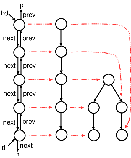
An example of a doubly-linked list and two of its spanning trees is shown in Fig. 2. Note that both the $\mathtt{next}$ and $\mathtt{prev}$ edges are local in both cases (they get mapped either to the $0$ or $-1$ direction) and so both of the spanning trees are local.

Notice that a spanning tree covers exactly the set of allocated locations in a state. Moreover, if a state $S$ has a spanning tree $t$ , then every location $\ell\in loc(S)$ , not necessarily allocated, is reachable from $t(\epsilon)$ by a chain of edges. In other words, the state does not contain garbage nodes.

Lemma 2

Let $S=\langle s,h\rangle$ be a state and $t$ its spanning tree. If all edges of $S$ are local with respect to $t$ , then for each spanning tree $t^{\prime}$ of $S$ we have $t\sim_{t^{\prime-1}\circ t}t^{\prime}$ , and, moreover, all edges of $S$ are local with respect to $t^{\prime}$ as well.

Proof

Let $p\in dom(t)$ be an arbitrary position and $d\in\mathcal{D}_{+}(t)$ be an arbitrary non-negative direction such that $p.d\in dom(t)$ . If $t$ is a spanning tree, then $t$ is bijective, and there exists a selector $s\in Sel$ such that $t(p)\xrightarrow{{\scriptstyle s}}t(p.d)$ is an edge in $S$ . Since $t^{\prime}$ is a spanning tree, it is also bijective, hence there exist $p^{\prime},p^{\prime\prime}\in dom(t^{\prime})$ such that $t^{\prime}(p^{\prime})=t(p)$ and $t^{\prime}(p^{\prime\prime})=t(p.d)$ .

By contradiction, suppose that $p^{\prime\prime}\neq p^{\prime}.e$ for all $e\in\mathcal{D}(t^{\prime})$ . Since $p^{\prime},p^{\prime\prime}\in dom(t^{\prime})$ , there exists a path $p^{\prime}=p_{1},\ldots,p_{k}$ such that $k>2$ , and, for all $1\leq i<k$ , we have $p_{i+1}=p_{i}.e_{i}$ , for some $e_{1},\ldots,e_{k-1}\in\mathcal{D}(t^{\prime})$ . Because $t^{\prime}$ is a spanning tree of $S$ , there exist selectors $s_{1},\ldots,s_{k-1}\in Sel$ such that one of the following holds, for all $1\leq i<k$ :

•

$t^{\prime}(p_{i})\xrightarrow{{\scriptstyle s_{i}}}t^{\prime}(p_{i+1})$ or
•

$t^{\prime}(p_{i+1})\xrightarrow{{\scriptstyle s_{i}}}t^{\prime}(p_{i})$ .

Since all the above edges of $S$ are local wrt. $t$ , there exists a path $p=(t^{-1}\circ t^{\prime})(p_{1}),\ldots,$ $(t^{-1}\circ t^{\prime})(p_{k})=p.d$ of pairwise distinct positions in $t$ , for $k>2$ , which contradicts with the fact that $t$ is a tree. In conclusion, for all $p\in dom(t)$ and $d\in\mathcal{D}_{+}(t)$ , such that $p.d\in dom(t)$ there exists $e\in\mathcal{D}(t^{\prime})$ such that $(t^{\prime-1}\circ t)(p.d)=(t^{\prime-1}\circ t)(p).e$ , and since $t^{\prime-1}\circ t$ is a bijective mapping, we have $t\sim_{t^{\prime-1}\circ t}t^{\prime}$ .

Finally, we are left with proving that all edges are local with respect to $t^{\prime}$ . Let $\ell\xrightarrow{{\scriptstyle s}}\ell^{\prime}$ be an arbitrary edge of $S$ , for some $s\in Sel$ . The edge is local with respect to $t$ , thus there exists $p\in dom(t)$ and $d\in\mathcal{D}(t)\cup\{\epsilon\}$ such that $t(p)=\ell$ and $t(p.d)=\ell^{\prime}$ . We distinguish three cases:

1.

If $d=\epsilon$ , then $p=p.d$ , and trivially $\ell=t^{\prime}((t^{\prime-1}\circ t)(p))=t^{\prime}((t^{\prime-1}\circ t)(p.d))=t^{\prime}((t^{\prime-1}\circ t)(p).d)=\ell^{\prime}$ .
2.

Otherwise, if $d\in\mathcal{D}_{+}(t)$ , taking into account that $t\sim_{t^{\prime-1}\circ t}t^{\prime}$ , by the first part of this lemma, we have $(t^{\prime-1}\circ t)(p.d)=(t^{\prime-1}\circ t)(p).e$ , for some $e\in\mathcal{D}(t^{\prime})$ . But $t^{\prime}((t^{\prime-1}\circ t)(p))=t(p)=\ell$ and $t^{\prime}((t^{\prime-1}\circ t)(p.d))=t(p.d)=\ell^{\prime}$ , so $\ell\xrightarrow{{\scriptstyle s}}\ell^{\prime}$ is local wrt. $t^{\prime}$ .
3.

Otherwise, if $d=-1$ , there exists $q\in dom(t)$ and $d^{\prime}\in\mathcal{D}_{+}(t)$ such that $p=q.d^{\prime}$ . Since $t\sim_{t^{\prime-1}\circ t}t^{\prime}$ , by the first part of this lemma, we have $(t^{\prime-1}\circ t)(q.d^{\prime})=(t^{\prime-1}\circ t)(q).e$ , for some $e\in\mathcal{D}(t^{\prime})$ . But $t^{\prime}(t^{\prime-1}\circ t)(q.d^{\prime})=t(p)=\ell$ and $t^{\prime}((t^{\prime-1}\circ t)(q))=t(q)=t(p.d)=\ell^{\prime}$ , so $\ell\xrightarrow{{\scriptstyle s}}\ell^{\prime}$ is local with respect to $t^{\prime}$ .

∎

As a consequence, if all edges of a state are local with respect to some spanning tree, they are also local with respect to any other spanning tree, hence we will simply say that they are local. A state is said to be local if it has only local edges.

2.3 Separation Logic

The syntax of basic formulae of Separation Logic (SL) is given below:

\begin{array}[]{lcl}\alpha&\in&Var\setminus\{\mathbf{nil}\};~x~\in~Var;\\ \Pi&::=&\alpha=x~|~\Pi_{1}\wedge\Pi_{2}\\ \Sigma&::=&\mathbf{emp}~|~\alpha\mapsto(x_{1},\ldots,x_{n})~|~\Sigma_{1}*\Sigma_{2}~\mbox{, for some}~n>0\\ \varphi&::=&\Sigma\wedge\Pi~|~\exists x~.~\varphi_{1}\end{array}

A formula of the form $\bigwedge_{i=1}^{n}\alpha_{i}=x_{i}$ defined by the $\Pi$ nonterminal in the syntax above is said to be pure. A formula of the form $\bigstar_{i=1}^{k}\alpha_{i}\mapsto(x_{i,1},\ldots,x_{i,n})$ defined by the $\Sigma$ nonterminal in the syntax above is said to be spatial. The atomic proposition $\mathbf{emp}$ denotes the empty spatial conjunction. A variable $x$ is said to be free in $\varphi$ if it does not occur under the scope of any existential quantifier. We denote by $FV(\varphi)$ the set of free variables, and by $AP(\varphi)$ the set of atomic propositions of $\varphi$ .

In the following, we shall use two equality relations. The syntactic equality, denoted $\alpha\equiv\beta$ , means that $\alpha$ and $\beta$ are the same syntactic object (formula, variable, tuples of variables, etc.). On the other hand, by writing $x=_{\Pi}y$ , for two variables $x,y\in Var$ and a pure formula $\Pi$ , we mean that the equality of the values of $x$ and $y$ is implied by $\Pi$ .

A substitution is an injective partial function $\sigma:Var\rightharpoonup_{fin}Var$ . Given a basic formula $\varphi$ and a substitution $\sigma$ , we denote by $\varphi[\sigma]$ the result of simultaneously replacing each variable (not necessarily free) $x$ that occurs in $\varphi$ , by $\sigma(x)$ . For instance, if $\sigma(x)=y$ , $\sigma(y)=z$ and $\sigma(z)=t$ , then $(\exists x,y~.~x\mapsto(y,z)\wedge z=x)[\sigma]\equiv\exists y,z~.~y\mapsto(z,t)~\wedge~t=y$ .

The semantics of a basic formula $\varphi$ is given by the relation $S\models\varphi$ , where $S=\langle s,h\rangle$ is a state such that $FV(\varphi)\subseteq dom(s)$ , and $\varphi$ is a basic SL formula. The definition of $\models$ is by induction on the structure of $\varphi$ :

\begin{array}[]{lcl}S\models\mathbf{emp}&\iff&dom(h)=\emptyset\\ S\models\alpha\mapsto(x_{1},\ldots,x_{n})&\iff&s=\{(\alpha,\ell_{0}),(x_{1},\ell_{1}),\ldots,(x_{n},\ell_{n})\}~\mbox{and}\\ &&h=\{\langle\ell_{0},\lambda i~.~\mbox{if}~1\leq i\leq n~\mbox{then}~\ell_{i}~\mbox{else}~\bot\rangle\}\\ &&~\mbox{for some $\ell_{0},\ell_{1},\ldots,\ell_{n}\in Loc$}\\ S\models\varphi_{1}*\varphi_{2}&\iff&S_{1}\models\varphi_{1}~\mbox{and}~S_{2}\models\varphi_{2}~\mbox{where $S_{1}\uplus S_{2}=S$}\\ S\models\exists x~.~\varphi&\iff&\langle s[x\leftarrow\ell],h\rangle\models\varphi~\mbox{for some $\ell\in Loc$}\end{array}

The semantics of $=$ and $\wedge$ is classical in first order logic. Note that we adopt here the strict semantics, in which a points-to relation $\alpha\mapsto(x_{1},\ldots,x_{n})$ holds in a state consisting of a single cell pointed to by $\alpha$ , with exactly $n$ outgoing edges $s(\alpha)\xrightarrow{{\scriptstyle k}}_{{\scriptstyle S}}s(x_{k})$ , $1\leq k\leq n$ , towards either the single allocated location (if $s(x_{k})=s(\alpha)$ ), or dangling locations (if $s(x_{k})\neq s(\alpha)$ ). The empty heap is specified by $\mathbf{emp}$ .

A variable $x\in FV(\Sigma)$ is said to be allocated in a basic spatial formula $\Sigma$ if it occurs on the right hand side of a points-to atomic proposition $x\mapsto(y_{0},\ldots,y_{k-1})$ of $\Sigma$ . If $\Sigma$ is satisfiable, then clearly each free variable $x\in FV(\Sigma)$ is allocated at most once. For a basic quantifier-free SL formula $\varphi\equiv\Sigma\wedge\Pi$ and two variables $x,y\in FV(\varphi)$ , we say that $y$ is $\varphi$ -reachable from $x$ in iff there exists a sequence $x=_{\Pi}\alpha_{0},\ldots,\alpha_{m}=_{\Pi}y$ , for some $m\geq 0$ , such that, for each $0\leq i<m$ , $\alpha_{i}\mapsto(\beta_{i,1},\ldots,\beta_{i,p_{i}})$ is a points-to proposition in $\Sigma$ , and $\beta_{i,s}=_{\Pi}\alpha_{i+1}$ , for some $1\leq s\leq p_{i}$ . A variable $x\in FV(\Sigma)$ is said to be a root of $\Sigma$ if every variable $y\in FV(\Sigma)$ is reachable from $x$ .

Remark.

Notice that there is no explicit disequality between variables in the basic fragment of SL. This is in part justified by the fact that disequality can be partially defined using the following implication: $\alpha\mapsto(x_{1},\ldots,x_{n})*\beta\mapsto(y_{1},\ldots,y_{m})\Rightarrow\alpha\neq\beta$ . This implication enforces disequality only between allocated variables. However, in practice, most SL specifications do not impose disequality constraints on dangling variables.

2.4 Inductive Definitions

A system of inductive definitions²² 2 The name inductive suggests that every structure described by the system is finite. (inductive system) $\mathcal{P}$ is a set of rules of the form:

\begin{array}[]{rcl}P_{1}(x_{1,1},\ldots,x_{1,n_{1}})&\equiv&\mid_{j=1}^{m_{1}}R_{1,j}(x_{1,1},\ldots,x_{1,n_{1}})\\ &\ldots&\\ P_{k}(x_{k,1},\ldots,x_{k,n_{k}})&\equiv&\mid_{j=1}^{m_{k}}R_{k,j}(x_{k,1},\ldots,x_{k,n_{k}})\end{array}

(1)

where $\{P_{1},\ldots,P_{k}\}$ is a set of predicates, $x_{i,1},\ldots,x_{i,n_{i}}$ are called formal parameters, and the formulae $R_{i,j}$ are called the rules of $P_{i}$ . Concretely, each rule is of the form:

R_{i,j}({\bf{x}})\equiv\exists{\bf{z}}~.~\Sigma*P_{i_{1}}({\bf{y}}_{1})*\ldots*P_{i_{m}}({\bf{y}}_{m})~\wedge~\Pi

where ${\bf{x}}\cap{\bf{z}}=\emptyset$ , and all of the following hold:

1.

$\mathbf{head}(R_{i,j})\stackrel{{\scriptstyle\scriptscriptstyle{def}}}{{\equiv}}\Sigma$ is a non-empty spatial formula (i.e. $\Sigma\not\equiv\mathbf{emp}$ ), and $FV(\Sigma)\subseteq{\bf{x}}\cup{\bf{z}}$ ,
2.

$\mathbf{tail}(R_{i,j})\stackrel{{\scriptstyle\scriptscriptstyle{def}}}{{\equiv}}\langle P_{i_{1}}({\bf{y}}_{1}),\ldots,P_{i_{m}}({\bf{y}}_{m})\rangle$ is an ordered sequence of predicate occurrences, where ${\bf{y}}_{1}\cup\ldots\cup{\bf{y}}_{m}\subseteq{\bf{x}}\cup{\bf{z}}$ ,
3.

$\Pi$ is a pure formula, and $FV(\Pi)\subseteq{\bf{z}}\cup{\bf{x}}$ . In the following, we restrict the pure part of each rule such that, for all formal parameters $\beta\in{\bf{x}}$ , we allow only equalities of the form $\alpha=_{\Pi}\beta$ , where $\alpha$ is allocated in $\Sigma$ . This restriction is of technical nature (see Section 4.1). It is possible to lift it, but only at the expense of an exponential blowup in the size of the resulting tree automaton.
4.

For all $1\leq r,s\leq m$ , if $x_{i,k}\in{\bf{y}}_{r}$ , $x_{i,l}\in{\bf{y}}_{s}$ , and $x_{i,k}=_{\Pi}x_{i,l}$ , for some $1\leq k,l\leq n_{i}$ , then $r=s$ . In other words, a formal parameter of a rule cannot be passed to two or more subsequent occurrences of predicates in that rule. This technical restriction can be lifted at the cost of introducing expensive tests for double allocation as was done in the translation of the inductive definitions to Monadic Second-Order Logic on graphs, reported in [13].

The size of a rule $R$ is denoted by ${|{R}|}$ and is defined inductively as follows:

\begin{array}[]{ccccc}{|{\alpha=x}|}=1&&{|{\mathbf{emp}}|}=1&&{|{\alpha\mapsto(x_{1},\ldots,x_{n})}|}=n+1\\ {|{\varphi\bullet\psi}|}={|{\varphi}|}+{|{\psi}|}&&{|{\exists x~.~\varphi}|}={|{\varphi}|}+1&&{|{P(x_{1},\ldots,x_{n})}|}=n\end{array}

where $\alpha\in Var\setminus\{\mathbf{nil}\}$ , $x,x_{1},\ldots,x_{n}\in Var$ , and $\bullet\in\{*,\wedge\}$ . The size of an inductive system $\mathcal{P}=\{P_{i}\equiv|_{j=1}^{m_{i}}R_{i,j}\}_{i=1}^{n}$ is defined as ${|{\mathcal{P}}|}=\sum_{i=1}^{n}\sum_{j=1}^{m_{i}}{|{R_{i,j}}|}$ .

Example 1

To illustrate the use inductive definitions (with the above restrictions), we first show how to define a predicate $\mathtt{DLL}(hd,p,tl,n)$ describing doubly-linked lists of length at least one. As depicted on the left of Fig. 2, the formal parameter $hd$ points to the first allocated node of such a list, $p$ to the node pointed by the $prev$ selector of $hd$ , $tl$ to the last node of the list (possibly equal to $hd$ ), and $n$ to the node pointed by the $next$ selector from $tl$ . This predicate can be defined as follows:

\mathtt{DLL}(hd,p,tl,n)\equiv hd\mapsto(n,p)~\wedge~hd=tl~\mid~\exists x.~hd\mapsto(x,p)*\mathtt{DLL}(x,hd,tl,n)\vskip-18.0pt

Example 2

Another example is the predicate $\mathtt{TLL}(root,ll,lr)$ describing binary trees with linked leaves, whose root is pointed by the $root$ formal parameter, the left-most leaf is pointed to by $ll$ , and the right-most leaf points to $lr$ (cf. Fig. 3):

\begin{array}[]{rcl}\mathtt{TLL}(root,ll,lr)&\equiv&root\mapsto(\mathbf{nil},\mathbf{nil},lr)~\wedge~root=ll\\ &&\mid~\exists x,y,z.~root\mapsto(x,y,\mathbf{nil})*\mathtt{TLL}(x,ll,z)*\mathtt{TLL}(y,z,lr)\end{array}

Remark.

The first restriction above ( $\mathbf{head}(R_{i,j})\not\equiv\mathbf{emp}$ ) currently does not allow defining data structures of zero size (such as empty lists, trees, etc.) and, more importantly, certain types of structure concatenation. For instance, considering the $\mathtt{DLL}$ predicate from the above example, the following predicate cannot be defined in our framework³³ 3 However, defining concatenation of trees with linked leaves is possible when the root is allocated: $\mathtt{JOIN\_TLL}(root,ll,lr)\equiv\exists x,y,z~.~root\mapsto(x,y,\mathbf{nil})*\mathtt{TLL}(x,ll,z)*\mathtt{TLL}(y,z,lr)$ .:

\mathtt{JOIN\_DLL}(hd,p,tl,n)\equiv\exists x,y~.~\mathtt{DLL}(hd,p,x,y)*\mathtt{DLL}(x,y,tl,n)

An extension to handle such definitions is possible, by introducing a special “concatenation” operation at the level of tree automata, which is considered for further investigation. ∎

Definition 4

Given a system $\mathcal{P}=\{P_{i}\equiv|_{j=1}^{m_{i}}R_{i,j}\}_{i=1}^{n}$ of inductive definitions, a rule $R_{i,j}(x_{i,1},\ldots,x_{i,k})\equiv\exists{\bf{z}}~.~\Sigma*P_{i_{1}}({\bf{y}}_{1})*\ldots*P_{i_{m}}({\bf{y}}_{m})\wedge\Pi$ is connected if and only if there exists a formal parameter $x_{i,\ell}$ , $1\leq\ell\leq k$ such that:

•

$x_{i,\ell}$ is a root of $\Sigma$ , and
•

for each $j=1,\ldots,m$ , there exists $0\leq s<{|{{\bf{y}}_{j}}|}$ such that $({\bf{y}}_{j})_{s}$ is $\Sigma\wedge\Pi$ -reachable from $x_{i,\ell}$ , and $x_{i_{j},s}$ is a root of the head of each rule of $P_{i_{j}}$ .

An inductive system is said to be connected if all its rules are connected. In the rest of this section, we consider only connected systems. This condition is necessary, since later on it is proved that entailment between predicates of disconnected systems is undecidable, in general (Thm. 5.1 in Sec. 5). Notice that the $\mathtt{DLL}$ and $\mathtt{TLL}$ systems from Examples 1 and 2 are both connected.

2.5 Tree Automata

A (finite, non-deterministic, bottom-up) tree automaton (abbreviated as TA in the following) is a quadruple $A=\langle Q,\Sigma,\Delta,F\rangle$ , where $\Sigma$ is a finite alphabet, $Q$ is a finite set of states, $F\subseteq Q$ is a set of final states, $\Sigma$ is an alphabet, and $\Delta$ is a set of transition rules of the form $\sigma(q_{1},\ldots,q_{n})\rightarrow q$ , for $\sigma\in\Sigma$ , and $q,q_{1},\ldots,q_{n}\in Q$ . Given a tree automaton $A=\langle Q,\Sigma,\Delta,F\rangle$ , for each rule $\rho=(\sigma(q_{1},\ldots,q_{n})\xrightarrow{{\scriptstyle}}q)$ , we define its size as ${|{\rho}|}=n+1$ . The size of the tree automaton is ${|{A}|}=\sum_{\rho\in\Delta}{|{\rho}|}$ . A run of $A$ over a tree $t:{\bf\mathbb{N}}^{*}\rightharpoonup_{fin}\Sigma$ is a function $\pi:dom(t)\rightarrow Q$ such that, for each node $p\in dom(t)$ , where $q=\pi(p)$ , if $q_{i}=\pi(p.i)$ for $1\leq i\leq n$ , then $\Delta$ has a rule $(t(p))(q_{1},\ldots,q_{n})\rightarrow q$ . We write $t\stackrel{{\scriptstyle\pi}}{{\Longrightarrow}}q$ to denote that $\pi$ is a run of $A$ over $t$ such that $\pi(\epsilon)=q$ . We use $t\Longrightarrow q$ to denote that $t\stackrel{{\scriptstyle\pi}}{{\Longrightarrow}}q$ for some run $\pi$ . The language of a $A$ is defined as ${\mathcal{L}}({A})=\{t\mid\exists q\in F,~t\Longrightarrow q\}$ .

3 Tiles and Semantics of Inductive Definitions

A tile is a tuple $T=\langle\varphi,{\bf{x}}_{-1},{\bf{x}}_{0},\ldots,{\bf{x}}_{d-1}\rangle$ , for some $d\geq 0$ , where $\varphi$ is a basic SL formula and each ${\bf{x}}_{i}$ is a tuple of pairwise distinct variables, called a port, such that ${\bf{x}}_{i}\cap{\bf{x}}_{j}=\emptyset$ , for all $-1\leq i<j<d$ , and ${\bf{x}}_{-1}\cup{\bf{x}}_{0}\cup\ldots\cup{\bf{x}}_{d-1}\subseteq FV(\varphi)$ . The set of all tiles is denoted by $\mathcal{T}$ . The variables from ${\bf{x}}_{-1}$ are said to be incoming, the ones from ${\bf{x}}_{0},\ldots,{\bf{x}}_{d-1}$ , are said to be outgoing, and the ones from $\mathbf{par}(T)=FV(\varphi)\setminus({\bf{x}}_{-1}\cup{\bf{x}}_{0}\cup\ldots\cup{\bf{x}}_{d-1})$ are called parameters. The arity of a tile $T=\langle\varphi,{\bf{x}}_{-1},{\bf{x}}_{0},\ldots,{\bf{x}}_{d-1}\rangle$ is the number of outgoing ports, denoted by $\#(T)=d$ . In the following, we denote $\mathbf{form}(T)\equiv\varphi$ and $\mathbf{port}_{i}(T)\equiv{\bf{x}}_{i}$ , for all $i=-1,0,\ldots,d-1$ .

Given two tiles $T_{1}=\langle\varphi_{1},{\bf{x}}^{1}_{-1},{\bf{x}}^{1}_{0},\ldots,{\bf{x}}^{1}_{d-1}\rangle$ and $T_{2}=\langle\varphi_{2},{\bf{x}}^{2}_{-1},{\bf{x}}^{2}_{0},\ldots,{\bf{x}}^{2}_{e-1}\rangle$ such that $FV(\varphi_{1})\cap FV(\varphi_{2})=\emptyset$ , for some $0\leq i\leq d-1$ such that ${|{{\bf{x}}^{1}_{i}}|}={|{{\bf{x}}^{2}_{-1}}|}$ , we define their $i$ -composition:

\begin{array}[]{rcl}T_{1}\circledast_{i}T_{2}&=&\langle\psi,{\bf{x}}^{1}_{-1},{\bf{x}}^{1}_{0},\ldots{\bf{x}}^{1}_{i-1},{\bf{x}}^{2}_{0},\ldots,{\bf{x}}^{2}_{e-1},{\bf{x}}^{1}_{i+1},\ldots,{\bf{x}}^{1}_{d-1}\rangle\\ \mbox{where}~\psi&\equiv&\exists{\bf{x}}^{1}_{i}\exists{\bf{x}}^{2}_{-1}~.~\varphi_{1}*\varphi_{2}\wedge{\bf{x}}^{1}_{i}={\bf{x}}^{2}_{-1}.\end{array}

For a tree position $q\in{\bf\mathbb{N}}^{*}$ and a tile $T=\langle\varphi,{\bf{x}}_{-1},{\bf{x}}_{0},\ldots,$ ${\bf{x}}_{d-1}\rangle$ , we denote by $T^{q}$ the tile obtained by renaming every free variable $x\in{\bf{x}}_{-1}\cup{\bf{x}}_{0}\cup\ldots\cup{\bf{x}}_{d-1}$ by $x^{q}$ . Note that the parameters $x\in\mathbf{par}(T)$ are not changed by this renaming.

Definition 5

A tiled tree is a tree $t:{\bf\mathbb{N}}^{*}\rightharpoonup_{fin}\mathcal{T}$ such that, for all positions $p\in dom(t)$ , the following holds:

•

$\#_{t}(p)=\#(t(p))$ , i.e. the arity of $p$ equals the arity of its label in $t$ , and
•

for all $0\leq i<\#_{t}(p)$ , the $d$ -composition $t(p)^{p}~\circledast_{i}~t(p.i)^{p.i}$ is defined.

A tiled tree $t$ corresponds to a tile defined inductively, for any $p\in dom(t)$ , as:

\Phi(t,p)=t(p)^{p}\circledast_{0}\Phi(t,p.0)\circledast_{1}\Phi(t,p.1)~\ldots~\circledast_{\#(p)-1}\Phi(t,p.(\#_{t}(p)-1)).\vskip-2.84526pt

The tile $\Phi(t,\epsilon)$ is said to be the characteristic tile of $t$ and it is denoted in the following as $\Phi(t)$ . It can be easily shown, by induction on the structure of the tiled tree $t$ , that $\Phi(t)=\langle\psi,{\bf{x}}_{-1}\rangle$ , for an SL formula $\psi$ and an incoming port ${\bf{x}}_{-1}$ . In other words, $\Phi(t)$ has no outgoing ports. In this case, we write $S\models\Phi(t)$ for $S\models\psi$ .

Given an inductive system $\mathcal{P}=\{P_{i}\equiv|_{j=1}^{m_{i}}R_{i,j}\}_{i=1}^{n}$ of the form (1), for each rule $R_{i,j}({\bf{x}})\equiv\exists{\bf{u}}~.~\Sigma*P_{i_{0}}({\bf{y}}_{0})*\ldots*P_{i_{n-1}}({\bf{y}}_{d-1})~\wedge~\Pi$ , where ${\bf{x}}\cap{\bf{u}}=\emptyset$ , we define a tile $T_{i,j}=\langle\varphi,{\bf{x}},{\bf{z}}_{0},\ldots,{\bf{z}}_{d-1}\rangle$ , where ${\bf{z}}_{i}$ are disjoint from ${\bf{y}}_{j}$ , for all $0\leq i,j<d$ , and $\varphi=\exists{\bf{u}}~.~\Sigma\wedge\Pi~\wedge~\bigwedge_{i=0}^{d-1}{\bf{z}}_{i}={\bf{y}}_{i}$ .

Definition 6

Let $\mathcal{P}=\big\{P_{i}~\equiv~\mid_{j=1}^{m_{i}}R_{i,j}\big\}_{i=1}^{n}$ be an inductive system (1). An unfolding tree of $\mathcal{P}$ is a tiled tree $t:{\bf\mathbb{N}}^{*}\rightharpoonup_{fin}\mathcal{T}$ such that:

•

$t(\epsilon)=T_{i,j}$ , for some $1\leq j\leq m_{i}$ , and
•

for every position $p\in dom(t)$ , if $t(p)=T_{i,j}$ and $\mathbf{tail}(R_{i,j})=\langle P_{i_{0}},\ldots,P_{i_{d-1}}\rangle$ , where $d=\#(T_{i,j})$ , then for all $0\leq j<d$ , we have $t(p.j)=T_{i_{j},k}$ , for some $1\leq k\leq m_{i_{j}}$ .

If $t(\epsilon)=T_{i,j}$ , for some $1\leq j\leq m_{i}$ , we say that $t$ is $i$ -rooted.

We denote by $\mathcal{T}_{i}(\mathcal{P})$ the set of $i$ -rooted unfolding trees of $\mathcal{P}$ . The semantics of a predicate $P_{i}({\bf{x}})\in\mathcal{P}$ is defined as follows: $S\models P_{i}({\bf{x}})\iff S\models\Phi(t)$ , for some $t\in\mathcal{T}_{i}(\mathcal{P})$ . Given an inductive system $\mathcal{P}$ and two predicates $P_{i}(x_{1},\ldots,x_{n})$ and $P_{j}(y_{1},\ldots,y_{n})$ of $\mathcal{P}$ , with the same number of formal parameters $n$ , and a tuple of variables ${\bf{x}}$ , where ${|{{\bf{x}}}|}=n$ , the entailment problem is defined as follows: $P_{i}({\bf{x}})\models_{\mathcal{P}}P_{j}({\bf{x}})~:~\forall S~.~S\models P_{i}({\bf{x}})\Rightarrow S\models P_{j}({\bf{x}}).$ A rooted inductive system $\langle\mathcal{P},P_{i}\rangle$ is an inductive system $\mathcal{P}$ with a designated predicate $P_{i}\in\mathcal{P}$ . Two rooted systems $\langle\mathcal{P},P_{i}\rangle$ and $\langle\mathcal{Q},Q_{j}\rangle$ are said to be equivalent if and only if $P_{i}\models_{\mathcal{P}\cup\mathcal{Q}}Q_{j}$ and $Q_{j}\models_{\mathcal{P}\cup\mathcal{Q}}P_{i}$ .

Definition 7

A rooted inductive system $\langle\{P_{1},\ldots,P_{n}\},P_{i}\rangle$ is said to be local if and only if for each unfolding tree $t\in\mathcal{T}_{i}(\mathcal{P})$ and each state $S\models\Phi(t)$ , $S$ is local.

The locality problem asks, given an inductive system $\mathcal{P}=\{P_{1},\ldots,P_{n}\}$ , and an index $i=1,\ldots,n$ , whether the rooted system $\langle\mathcal{P},P_{i}\rangle$ is local. Our method for deciding entailment problems of the form $P_{i}\models_{\mathcal{P}}P_{j}$ is shown to be sound and complete provided that both $\langle\mathcal{P},P_{i}\rangle$ and $\langle\mathcal{P},P_{j}\rangle$ are local. Otherwise, if one system is not local, our method is sound, i.e. the algorithm returns “yes” only if the entailment holds. We describe further a canonization procedure (Sec. 4.1) which performs a sufficient locality test on the system, prior to the encoding of the inductive system as a tree automaton.

3.1 Canonical Tiles

This section defines a class of canonically tiled trees (or, to be short, canonical trees) intended to reduce the number of ways in which a given local state can be encoded. Moreover, it is shown that despite a local state can still be described by several different canonical trees, such trees must be in a rotation relation called a canonical rotation. This fact is the basis of the completeness argument of our method. By defining a closure of tree automata (accepting canonical trees of states described by a given inductive predicate) under canonical rotations, we ensure that any entailment between two local inductive predicates can be reduced to a language inclusion problem. The case of non-local states is subsequently dealt with in a sound (yet, in general, not complete) way in the next subsection (Sec. 3.2).

A tile $T=\langle\varphi,{\bf{x}}_{-1},{\bf{x}}_{0},\ldots,{\bf{x}}_{d-1}\rangle$ is said to be a singleton if $\varphi$ is of one of the forms:

1.

$\exists z~.~z\mapsto(y_{0},\ldots,y_{m-1})\wedge\Pi$ or
2.

$z\mapsto(y_{0},\ldots,y_{m-1})\wedge\Pi$ and $z\in\mathbf{par}(T)$

and the following holds:

•

For all $-1\leq i<d$ , ${\bf{x}}_{i}\cap(\{z,\mathbf{nil}\}\cup\mathbf{par}(T))=\emptyset$ , i.e. neither the incoming nor the outgoing tuples of variables contain $z$ , $\mathbf{nil}$ , or parameters.
•

For each $0\leq j<m$ , exactly one of the following holds: either (i) $y_{j}\equiv z$ , (ii) $y_{j}\equiv\mathbf{nil}$ , (iii) $y_{j}\in\mathbf{par}(T)$ , or (iv) there exists a unique tuple of variables ${\bf{x}}_{i}$ , $-1\leq i<d$ , such that $y_{j}$ occurs in ${\bf{x}}_{i}$ .
•

For each outgoing tuple of variables ${\bf{x}}_{i}$ , $0\leq i<d$ , there exists a variable $y_{j}\not\in\{z,\mathbf{nil}\}\cup\mathbf{par}(T)$ , for some $0\leq j<m$ , such that $y_{j}$ occurs in ${\bf{x}}_{i}$ .

We denote the spatial formula of a singleton tile as $(\exists z)~z\mapsto(y_{0},\ldots,y_{m-1})$ in order to account for the optional quantification of the allocated variable $z$ . A singleton tile $T=\langle(\exists z)~z\mapsto(y_{0},\ldots,y_{m-1})\wedge\Pi,~{\bf{x}}_{-1},{\bf{x}}_{0},\ldots,{\bf{x}}_{d-1}\rangle$ is said to be canonical if, moreover, for all $-1\leq i<d$ , ${\bf{x}}_{i}$ can be factorized as ${\bf{x}}_{i}\equiv{\bf{x}}^{fw}_{i}\cdot{\bf{x}}^{bw}_{i}$ such that:

1.

${\bf{x}}^{bw}_{-1}=\langle y_{h_{0}},\ldots,y_{h_{k}}\rangle$ , for some ordered sequence $0\leq h_{0}<\ldots<h_{k}<m$ , i.e. the incoming tuple is ordered by the selectors referencing its elements.
2.

For all $0\leq i<d$ , ${\bf{x}}^{fw}_{i}\equiv\langle y_{j_{0}},\ldots,y_{j_{k_{i}}}\rangle$ , for some ordered sequence $0\leq j_{0}<\ldots<j_{k}<m$ , i.e. each outgoing tuple is ordered by the selectors referencing its elements.
3.

For all $0\leq i,j<d$ , if $({\bf{x}}_{i}^{fw})_{0}\equiv y_{p}$ and $({\bf{x}}_{j}^{fw})_{0}\equiv y_{q}$ , for some $0\leq p<q<m$ , then $i<j$ , i.e. outgoing tuples are ordered by the selector referencing the first element.
4.

$({\bf{x}}_{-1}^{fw}\cup{\bf{x}}_{0}^{bw}\cup\ldots\cup{\bf{x}}_{d-1}^{bw})\cap\{y_{0},\ldots,y_{m-1}\}=\emptyset$ and $\Pi\equiv{\bf{x}}_{-1}^{fw}=z~\wedge~\bigwedge_{i=0}^{d-1}{\bf{x}}_{i}^{bw}=z$ .

Given a canonical tile $T=\langle(\exists z)~z\mapsto(y_{0},\ldots,y_{m-1})\wedge\Pi,~{\bf{x}}_{-1},{\bf{x}}_{0},\ldots,{\bf{x}}_{d-1}\rangle$ , the decomposition of each tuple ${\bf{x}}_{i}$ into ${\bf{x}}^{fw}_{i}$ and ${\bf{x}}^{bw}_{i}$ is unique. This is because ${\bf{x}}^{fw}_{i}$ contains all referenced variables $y_{j}$ that occur in an output port ${\bf{x}}_{i}$ (since ${\bf{x}}^{bw}_{i}\cap\{y_{0},\ldots,y_{m-1}\}=\emptyset$ ) in the same order in which they are referenced in $z\mapsto(y_{0},\ldots,y_{m-1})$ . The same holds for the input port ${\bf{x}}_{-1}$ , with the roles of ${\bf{x}}_{-1}^{fw}$ and ${\bf{x}}_{-1}^{bw}$ swapped. As each outgoing port must contain at least one such variable, by the definition of singleton tiles, we also have that ${\bf{x}}^{fw}_{i}\neq\emptyset$ , for all $0\leq i<d$ . We denote further by $\mathbf{port}^{fw}_{i}(T)$ and $\mathbf{port}^{bw}_{i}(T)$ the tuples ${\bf{x}}^{fw}_{i}$ and ${\bf{x}}^{bw}_{i}$ , resp., for all $i=-1,\ldots,d-1$ . The set of canonical tiles is denoted as $\mathcal{T}^{c}$ .

Definition 8

A tiled tree $t:{\bf\mathbb{N}}^{*}\rightharpoonup_{fin}\mathcal{T}^{c}$ is said to be canonical if and only if, for any $p\in dom(t)$ and each $0\leq i<\#_{t}(p)$ , we have ${|{\mathbf{port}^{fw}_{i}(t(p))}|}={|{\mathbf{port}^{fw}_{-1}(t(p.i))}|}$ and ${|{\mathbf{port}^{bw}_{i}(t(p))}|}={|{\mathbf{port}^{bw}_{-1}(t(p.i))}|}$ .

Example 3 (cont. of Ex. 1)

To illustrate the notion of canonical trees, Fig. 4 shows two canonical trees for a given DLL. The tiles are depicted as big rectangles containing the appropriate basic formula as well the input and output ports. In all ports, the first variable is in the forward and the second in the backward part.

We will now work towards the notion of canonical rotations. For that, we first give one technical definition. Given a canonical tree $t:{\bf\mathbb{N}}^{*}\rightharpoonup_{fin}\mathcal{T}^{c}$ , and a state $S=\langle s,h\rangle$ , let $u:dom(t)\rightarrow dom(h)$ be an arbitrary tree labeled with allocated locations from $S$ . For each position $p\in dom(t)$ its explicit neighbourhood with respect to $t$ and $u$ is the state $S_{\langle t,u,p\rangle}=\langle s_{p},h_{p}\rangle$ defined as follows:

•

$h_{p}=\overline{h}$ , and

•

s_{p}(x)=\left\{\begin{array}[]{ll}u(p)&\mbox{if $x\in\mathbf{port}_{-1}^{fw}(t(p))\cup\mathbf{port}_{0}^{bw}(t(p))\cup\ldots\cup\mathbf{port}_{\#_{t}(p)-1}^{bw}(t(p))$}\\ u(p.i)&\mbox{if $x\in\mathbf{port}_{i}^{fw}(t(p))$, for some $0\leq i<\#_{t}(p)$}\\ u(p.(-1))&\mbox{if $p\neq\epsilon$ and $x\in\mathbf{port}_{-1}^{bw}(t(p))$}\\ \overline{s}(x)&\mbox{otherwise}\end{array}\right.

where $S_{\langle u(p)\rangle}=\langle\overline{s},\overline{h}\rangle$ is the neighbourhood of the location $u(p)$ in $S$ .

An important property of canonical trees is that each state that is a model of the characteristic tile $\Phi(t)$ of a canonical tree $t$ (i.e. $S\models\Phi(t)$ ) can be uniquely described by a local spanning tree $u:dom(t)\rightarrow Loc$ , which has the same structure as $t$ , i.e. $dom(u)=dom(t)$ . An immediate consequence is that any two models of $\Phi(t)$ differ only by a renaming of the allocated locations, i.e. they are identical up to isomorphism.

Lemma 3

Let $t:{\bf\mathbb{N}}^{*}\rightharpoonup_{fin}\mathcal{T}^{c}$ be a canonical tree, and let $S=\langle s,h\rangle$ be a state. Then $S\models\Phi(t)$ iff there exists a local spanning tree $u:dom(t)\rightarrow dom(h)$ such that, for all $p\in dom(t)$ :

1.

${|{\mathbf{port}_{i}^{fw}(t(p))}|}={|\!|{\{k\in Sel~|~u(p)\xrightarrow{{\scriptstyle k}}_{{\scriptstyle S}}u(p.i)\}}|\!|}$ , for all $0\leq i<\#_{t}(p)$ .
2.

${|{\mathbf{port}_{-1}^{bw}(t(p))}|}={|\!|{\{k\in Sel~|~u(p)\xrightarrow{{\scriptstyle k}}_{{\scriptstyle S}}u(p.(-1))\}}|\!|}$ if $p\neq\epsilon$ .
3.

$S_{\langle t,u,p\rangle}\models\mathbf{form}(t(p))$ .

Proof

“ $\Rightarrow$ ” By induction on the structure of $t$ . For the base case $\#_{t}(\epsilon)=0$ , i.e. $dom(t)=\{\epsilon\}$ , we have $t(\epsilon)=\langle\mathbf{form}(t(\epsilon),\mathbf{port}_{-1}(t(\epsilon))\rangle$ and therefore $S\models\Phi(t)$ if and only if $S\models\mathbf{form}(t(\epsilon))$ . Since $t(\epsilon)$ is a canonical tile, only one location is allocated in $dom(h)$ , i.e. $dom(h)=\{\ell\}$ , for some $\ell\in Loc$ . We define $u=\{(\epsilon,\ell)\}$ . It is immediate to check that $u$ is a local spanning tree of $S$ , and that $S_{\langle t,u,\epsilon\rangle}=S\models\mathbf{form}(t(\epsilon))$ – points (1) and (2) are vacuously true.

For the induction step $\#_{t}(\epsilon)=d>0$ , we have:

\Phi(t,\epsilon)=t(\epsilon)^{\epsilon}\circledast_{0}\Phi(t,0)\ldots\circledast_{d-1}\Phi(t,d-1)

Since $S\models\Phi(t,\epsilon)$ , there exist states $S_{i}=\langle s_{i},h_{i}\rangle$ , for each $-1\leq i<d$ , such that $S_{-1}\models t(\epsilon)^{\epsilon}$ and $S_{i}\models\Phi(t,i)$ , for all $0\leq i<d$ , and moreover, $S=S_{-1}\uplus S_{0}\uplus\ldots\uplus S_{d-1}$ . By the induction hypothesis, for each $0\leq i<d$ there exists a local spanning tree $u_{i}:dom({{t}}_{|_{{i}}})\rightarrow dom(h_{i})$ , meeting conditions (1), (2) and (3). Since $S_{-1}\models t(\epsilon)^{\epsilon}$ , it must be that $dom(h_{-1})=\{\ell\}$ for some location $\ell\in Loc$ . We define $u$ as follows:

\begin{array}[]{rcl}u(\epsilon)&=&\ell\\ u(i.q)&=&u_{i}(q)~\mbox{for all $q\in dom(u_{i})$}\end{array}

To prove that $u$ is a spanning tree of $S$ , let $p\in dom(u)$ be a position, and $0\leq i<\#_{u}(p)$ be a direction. We distinguish two cases:

•

if $p=\epsilon$ , then $\mathbf{port}_{i}^{fw}(t(p))\neq\emptyset$ , hence there exists an edge $\ell\xrightarrow{{\scriptstyle k}}_{{\scriptstyle S_{-1}}}u_{i}(\epsilon)$ . Then $u(p)\xrightarrow{{\scriptstyle k}}_{{\scriptstyle S}}u(p.i)$ as well.
•

if $p=j.q$ , and $q\in dom(u_{j})$ , for some $0\leq j<d$ , by the induction hypothesis, there exists $k\in Sel$ , such that $u(p)=u_{j}(q)\xrightarrow{{\scriptstyle k}}_{{\scriptstyle S_{j}}}u_{j}(q.i)=u(p.i)$ , i.e. $u(p)\xrightarrow{{\scriptstyle k}}_{{\scriptstyle S}}u(p.i)$ .

To prove that $u$ is a local spanning tree of $S$ , let $\kappa\xrightarrow{{\scriptstyle k}}_{{\scriptstyle S}}\kappa^{\prime}$ be an edge, for some $\kappa,\kappa^{\prime}\in dom(h)$ . Since $dom(h)$ is a disjoint union of $dom(h_{-1})=\{\ell\},dom(h_{0}),\ldots,dom(h_{d-1})$ , we distinguish several cases:

•

if $\kappa\in dom(h_{-1})$ and $\kappa^{\prime}\in dom(h_{i})$ , for some $0\leq i<d$ , then $u(p)=\kappa=\ell$ and $u(i)=u_{i}(\epsilon)=\kappa^{\prime}$ is the only possibility – due to the strict semantics of SL, it is not possible to define an edge between $\ell$ and an location $\kappa^{\prime}=u_{i}(q)$ , unless $q=\epsilon$ .
•

if $\kappa,\kappa^{\prime}\in dom(h_{i})$ , for some $0\leq i<d$ , then, by the induction hypothesis, there exists $q\in dom(u_{i})$ and $0\leq j<\#_{u_{i}}(q)$ such that $\kappa=u_{i}(q)=u(i.q)$ and $\kappa^{\prime}=u_{i}(q.j)=u(i.q.j)$ .
•

if $\kappa\in dom(h_{i})$ and $\kappa^{\prime}\in dom(h_{j})$ , for some $0\leq i,j<d$ , then we reach a contradiction with the strict semantics of SL – since there is no equality between output ports in $t(\epsilon)$ , it is not possible to define an edge between a location from $dom(h_{i})$ and $dom(h_{j})$ ,

The proofs of points (1), (2) and (3) are by the strict semantics of SL.

“ $\Leftarrow$ ” By induction on the structure of $t$ . In the base case $\#_{t}(\epsilon)=0$ , i.e. $dom(t)=\{\epsilon\}$ , then $t(\epsilon)=\langle\mathbf{form}(t(\epsilon),\mathbf{port}_{-1}(t(\epsilon))\rangle$ . We have $S=S_{\langle t,u,\epsilon\rangle}\models\mathbf{form}(t(\epsilon))$ , by point (3), hence $S\models\Phi(t)$ .

For the induction step $\#_{t}(\epsilon)=d>0$ , let $u_{i}={{u}}_{|_{{i}}}$ , for all $0\leq i<d$ . Since $u$ is a bijective function, we have $img(u_{i})\cap img(u_{j})=\emptyset$ , for all $0\leq i<j<d$ . For all $-1\leq i<d$ , we define $S_{i}=\langle s_{i},h_{i}\rangle$ , where:

\begin{array}[]{rclr}h_{i}(\ell)&=&\left\{\begin{array}[]{ll}h(\ell)&\mbox{if $\ell\in img(u_{i})$}\\ \bot&\mbox{otherwise}\end{array}\right.&~\mbox{for all $\ell\in Loc$, if $i\geq 0$}\\ h_{-1}(\ell)&=&\left\{\begin{array}[]{ll}h(\ell)&\mbox{if $u(\epsilon)=\ell$}\\ \bot&\mbox{otherwise}\end{array}\right.&~\mbox{for all $\ell\in Loc$}\\ s_{i}(x)&=&\left\{\begin{array}[]{ll}s(x)&\mbox{if $s(x)\in Img(h_{i})$}\\ \bot&\mbox{otherwise}\end{array}\right.&~\mbox{for all $x\in Var$}\end{array}

It is not hard to show that $S=S_{-1}\uplus S_{0}\uplus\ldots S_{d-1}$ . Since $u$ is a local spanning tree of $S$ , $u_{i}$ is a local spanning tree for $S_{i}$ , for all $0\leq i<d$ , and conditions (1), (2) and (3) hold for $S_{i}$ and $u_{i}$ , respectively. By the induction hypothesis, we have $S_{i}\models\Phi({{t}}_{|_{{i}}},\epsilon)$ . By points (1), (2) and (3) moreover, we have that $S_{-1}\models\mathbf{form}(t(\epsilon))$ . Hence $S\models\Phi(t)$ . ∎

The following definition is a refinement of Def. 2. The change in the structure of the tree is mirrored by a change in the structure of the canonical tiles labeling the tree.

Definition 9

Given two canonical trees $t,u:{\bf\mathbb{N}}^{*}\rightharpoonup_{fin}\mathcal{T}^{c}$ , we say that $u$ is a canonical rotation of $t$ , denoted $t\sim_{r}^{c}u$ , if and only if $r:dom(t)\rightarrow dom(u)$ is a bijective function, and for all $p\in dom(t)$ , there exists a substitution $\sigma_{p}:Var\rightharpoonup_{fin}Var$ such that $\mathbf{form}(t(p))[\sigma_{p}]\equiv\mathbf{form}(u(r(p)))$ , and for all $0\leq i<\#_{t}(p)$ , there exists $j\in\mathcal{D}(u)$ such that $r(p.i)=r(p).j$ , and:

\begin{array}[]{rcl}\mathbf{port}_{i}^{fw}(t(p))[\sigma_{p}]&\equiv&\mathbf{if}~j\geq 0~\mathbf{then}~\mathbf{port}_{j}^{fw}(u(r(p)))~\mathbf{else}~\mathbf{port}_{-1}^{bw}(u(r(p)))\\ \mathbf{port}_{i}^{bw}(t(p))[\sigma_{p}]&\equiv&\mathbf{if}~j\geq 0~\mathbf{then}~\mathbf{port}_{j}^{bw}(u(r(p)))~\mathbf{else}~\mathbf{port}_{-1}^{fw}(u(r(p)))\end{array}

Example 4 (cont. of Ex. 3)

The notion of canonical rotation is illustrated by the canonical rotation $r$ relating the two canonical trees of a DLL shown in Fig. 4. In its case, the variable substitutions are simply the identity in each node. Note, in particular, that when the tile $0$ of the left tree (i.e., the second one from the top) gets rotated to the tile $1$ of the right tree (i.e., the right successor of the root), the input and output ports get swapped and so do their forward and backward parts.

The following lemma is the key for proving completeness of our entailment checking for local inductive systems: if a (local) state is a model of the characteristic tiles of two different canonical tree, then these trees must be related by canonical rotation.

Lemma 4

Let $t:{\bf\mathbb{N}}^{*}\rightharpoonup_{fin}\mathcal{T}^{c}$ be a canonical tree and $S=\langle s,h\rangle$ be a state such that $S\models\Phi(t)$ . Then, for any canonical tree $u:{\bf\mathbb{N}}^{*}\rightharpoonup_{fin}\mathcal{T}^{c}$ , we have $S\models\Phi(u)$ iff $t\sim^{c}u$ .

Proof

If $S\models\Phi(t)$ , there exists a local spanning tree $t_{s}:dom(t)\rightarrow dom(h)$ of $S$ , that meets the three conditions of Lemma 3.

“ $\Rightarrow$ ” If $S\models\Phi(u)$ there exists a local spanning tree $u_{s}:dom(u)\rightarrow dom(h)$ of $S$ , that meets the three conditions of Lemma 3. Since $t_{s}$ and $u_{s}$ are spanning trees of $S$ , by Lemma 2, we have $t_{s}\sim_{u_{s}^{-1}\circ t_{s}}u_{s}$ . Let $r=u_{s}^{-1}\circ t_{s}$ from now on. Clearly, for any $p\in dom(t)$ , we have $t_{s}(p)=u_{s}(r(p))$ . Since $dom(t)=dom(t_{s})$ and $dom(u)=dom(u_{s})$ , we have $t\sim_{r}u$ as well.

We further need to prove the three points of Def. 9 in order to show that $t\sim_{r}^{c}u$ . Let $p\in dom(t)$ be an arbitrary location. For the first two points, let $0\leq i<\#_{t}(p)$ be a direction. We have $t_{s}(p.i)=u_{s}(r(p.i))=u_{s}(r(p).j)$ , for some $j\in\mathcal{D}(u)$ . We distinguish two cases:

•

if $j\geq 0$ , we compute:

\begin{array}[]{rcl}{|{\mathbf{port}_{i}^{fw}(t(p))}|}&=&{|\!|{\{k\in Sel~|~t_{s}(p)\xrightarrow{{\scriptstyle k}}_{{\scriptstyle S}}t_{s}(p.i)\}}|\!|}\\ &=&{|\!|{\{k\in Sel~|~u_{s}(r(p))\xrightarrow{{\scriptstyle k}}_{{\scriptstyle S}}u_{s}(r(p).j)\}}|\!|}\\ &=&{|{\mathbf{port}_{j}^{fw}(u(r(p)))}|}\\ \\ {|{\mathbf{port}_{i}^{bw}(t(p))}|}&=&{|{\mathbf{port}_{-1}^{bw}(t(p.i))}|}~\mbox{(by Def. \ref{Canonically-tiled})}\\ &=&{|\!|{\{k\in Sel~|~t_{s}(p.i)\xrightarrow{{\scriptstyle k}}_{{\scriptstyle S}}t_{s}(p)\}}|\!|}\\ &=&{|\!|{\{k\in Sel~|~u_{s}(r(p).j)\xrightarrow{{\scriptstyle k}}_{{\scriptstyle S}}u_{s}(r(p))\}}|\!|}\\ &=&{|{\mathbf{port}_{j}^{bw}(u(r(p)))}|}\end{array}

•

if $j=-1$ , we compute:

\begin{array}[]{rcl}{|{\mathbf{port}_{i}^{fw}(t(p))}|}&=&{|\!|{\{k\in Sel~|~u_{s}(r(p))\xrightarrow{{\scriptstyle k}}_{{\scriptstyle S}}u_{s}(r(p).(-1))\}}|\!|}\\ &=&{|{\mathbf{port}_{-1}^{bw}(u(r(p)))}|}\\ \\ {|{\mathbf{port}_{i}^{bw}(t(p))}|}&=&{|\!|{\{k\in Sel~|~u_{s}(r(p).(-1))\xrightarrow{{\scriptstyle k}}_{{\scriptstyle S}}u_{s}(r(p))\}}|\!|}\\ &=&{|\!|{\{k\in Sel~|~u_{s}(r(p).(-1))\xrightarrow{{\scriptstyle k}}_{{\scriptstyle S}}u_{s}(r(p).(-1).j^{\prime})\}}|\!|}\\ &&~\mbox{for some $j^{\prime}\geq 0$ such that $r(p)=r(p).(-1).j^{\prime}$}\\ &=&{|{\mathbf{port}_{j^{\prime}}^{fw}(u(r(p).(-1)))}|}\\ &=&{|{\mathbf{port}_{-1}^{fw}(u(r(p)))}|}~\mbox{(by Def. \ref{Canonically-tiled})}\end{array}

Since all variables are pairwise distinct in $\mathbf{port}_{i}(t(p))$ and $\mathbf{port}_{j}(u(r(p)))$ , respectively, one can define a substitution $\sigma_{p}$ meeting the conditions of the first two points of Def. 9.

For the third point of Def. 9, by Lemma 3, we have that $S_{\langle t,t_{s},p\rangle}\models\mathbf{form}(t(p))$ and $S_{\langle u,u_{s},r(p)\rangle}\models\mathbf{form}(u(r(p)))$ , where $S_{\langle t,t_{s},p\rangle}=\langle s_{t},h_{t}\rangle$ is the explicit neighbourhood of $p$ w.r.t $t$ and $t_{s}$ , and $S_{\langle u,u_{s},p\rangle}=\langle s_{u},h_{u}\rangle$ is the explicit neighbourhood of $r(p)$ w.r.t $u$ and $u_{s}$ . Since $t(p)$ and $u(r(p))$ are canonical tiles, we have:

\begin{array}[]{rcl}\mathbf{form}(t(p))&\equiv&(\exists z)~z\mapsto(y_{0},\ldots,y_{m-1})\wedge\Pi_{t}\\ \mathbf{form}(u(r(p)))&\equiv&(\exists w)~w\mapsto(v_{0},\ldots,v_{n-1})\wedge\Pi_{u}\end{array}

where

\begin{array}[]{rcl}\Pi_{t}&\equiv&\mathbf{port}_{-1}^{fw}(t(p))=z~\wedge~\bigwedge_{i=0}^{\#_{t}(p)-1}\mathbf{port}_{i}^{bw}(t(p))=z\\ \Pi_{u}&\equiv&\mathbf{port}_{-1}^{fw}(u(r(p)))=w~\wedge~\bigwedge_{i=0}^{\#_{u}(r(p))-1}\mathbf{port}_{i}^{bw}(u(r(p)))=w\end{array}

We extend the substitution $\sigma_{p}$ to $\sigma_{p}[z\leftarrow w]$ in the following. It is not hard to check that $s_{t}\circ\sigma_{p}=s_{u}$ and $h_{t}=h_{u}$ . Hence $S_{\langle u,u_{s},p\rangle}\models\mathbf{form}(t(p))[\sigma_{p}]$ . Since both $\mathbf{form}(t(p))[\sigma_{p}]$ and $\mathbf{form}(u(r(p)))$ have the same model, by the definition of the (strict) semantics of SL, it follows that the numbers of edges are the same, i.e. $m=n$ , and either both $z$ and $w$ are quantified, or they are free. Thus, we obtain that $\mathbf{form}(t(p))[\sigma_{p}]\equiv\mathbf{form}(u(r(p)))$ .

” $\Leftarrow$ ” It $t\sim^{c}u$ , there exists a bijective function $r:dom(t)\rightarrow dom(u)$ , meeting the conditions of Def. 9. Let $u_{s}=t_{s}\circ r^{-1}$ be a tree. Since $t_{s}$ and $r$ are bijective, then also $u_{s}$ is bijective, and $dom(u_{s})=dom(u)$ . To prove that $S\models\Phi(u)$ , it is enough to show that $u_{s}$ is a local spanning tree of $S$ , meeting the three conditions of Lemma 3.

To show that $u_{s}$ is a local spanning tree of $S$ , let $p\in dom(u_{s})$ and $i\in\mathcal{D}_{+}(u_{s})$ such that $p.i\in dom(u_{s})$ . Since $t_{s}\sim_{r}u_{s}$ , by Prop. 1, we have $u_{s}\sim_{r^{-1}}t_{s}$ , hence there exists $j\in\mathcal{D}(t_{s})$ such that $r^{-1}(p.i)=r^{-1}(p).j$ . Since $t_{s}$ is a spanning tree of $S$ , there exists a selector $k\in Sel$ such that:

u_{s}(p)=t_{s}(r^{-1}(p))\xrightarrow{{\scriptstyle k}}_{{\scriptstyle S}}t_{s}(r^{-1}(p).j)=t_{s}(r^{-1}(p.i))=u_{s}(p.i)

Hence $u_{s}$ is a spanning tree of $S$ . In order to prove its locality, let $\ell\xrightarrow{{\scriptstyle k}}\ell^{\prime}$ be an edge of $S$ , for some $\ell,\ell\in loc(S)$ and $k\in Sel$ . Since $t_{s}$ is a local spanning tree of $S$ , there exist $p\in dom(t_{s})$ and $i\in\mathcal{D}_{+}(t_{s})$ such that $\ell=t_{s}(p)=u_{s}(r(p))$ and $\ell^{\prime}=t_{s}(p.i)=u_{s}(r(p.i))$ . Since $t_{s}\sim_{r}u_{s}$ , there exists $j\in\mathcal{D}(u_{s})$ such that $r(p.i)=r(p).j$ . Hence we have $u_{s}(r(p))=\ell\xrightarrow{{\scriptstyle k}}\ell^{\prime}=u_{s}(r(p).j)$ , i.e. the edge is local w.r.t. $u_{s}$ as well.

To prove point (1) of Lemma 3, let $p\in dom(u)$ be an arbitrary position, and $0\leq i<\#_{u}(p)$ be a direction. Since $u_{s}\sim_{r^{-1}}t_{s}$ , we have $r^{-1}(p.i)=r^{-1}(p).j$ , for some $j\in\mathcal{D}(t)$ . We compute:

\begin{array}[]{rcl}{|\!|{\{k\in Sel~|~u_{s}(p)\xrightarrow{{\scriptstyle k}}_{{\scriptstyle S}}u_{s}(p.i)\}}|\!|}&=&{|\!|{\{k\in Sel~|~t_{s}(r^{-1}(p))\xrightarrow{{\scriptstyle k}}_{{\scriptstyle S}}t_{s}(r^{-1}(p.i)\}}|\!|}\\ &=&{|\!|{\{k\in Sel~|~t_{s}(r^{-1}(p))\xrightarrow{{\scriptstyle k}}_{{\scriptstyle S}}t_{s}(r^{-1}(p).j)\}}|\!|}\end{array}

We distinguish two cases:

•

if $j\geq 0$ , we have, by Lemma 3 applied to $t$ and $t_{s}$ :

\begin{array}[]{rcl}{|\!|{\{k\in Sel~|~t_{s}(r^{-1}(p))\xrightarrow{{\scriptstyle k}}_{{\scriptstyle S}}t_{s}(r^{-1}(p).j)\}}|\!|}&=&{|{\mathbf{port}_{j}^{fw}(t(r^{-1}(p)))}|}\\ &=&{|{\mathbf{port}_{i}^{fw}(u(p))}|}\end{array}

The last equality is because $r(r^{-1}(p).j)=r(r^{-1}(p)).i$ .

•

if $j=-1$ , there exists $d\in\mathcal{D}_{+}(t)$ such that $r^{-1}(p)=(r^{-1}(p).(-1)).d$ . But then we have:

\begin{array}[]{rcl}r((r^{-1}(p).(-1)).d)&=&r(r^{-1}(p))=p=(p.i).(-1)\\ &=&r(r^{-1}(p).(-1)).(-1)\end{array}

We compute, further:

\begin{array}[]{rcl}{|\!|{\{k\in Sel~|~t_{s}(r^{-1}(p))\xrightarrow{{\scriptstyle k}}_{{\scriptstyle S}}t_{s}(r^{-1}(p).j)\}}|\!|}&=&{|{\mathbf{port}_{-1}^{bw}(t(r^{-1}(p)))}|}\\ &=&{|{\mathbf{port}_{d}^{bw}(t(r^{-1}(p).(-1)))}|}~\mbox{(by Def. \ref{Canonically-tiled})}\\ &=&{|{\mathbf{port}_{-1}^{fw}(u(p.i))}|}~\mbox{(by Def. \ref{Canonical-rotation})}\\ &=&{|{\mathbf{port}_{i}^{fw}(u(p))}|}~\mbox{(by Def. \ref{Canonically-tiled})}\end{array}

For point (2) of Lemma 3, one applies a symmetrical argument. To prove point (3) of Lemma 3, let $S_{\langle t,t_{s},r^{-1}(p)\rangle}=\langle s_{t},h_{t}\rangle$ be the explicit neighbourhood of $r^{-1}(p)$ w.r.t $t$ and $t_{s}$ . It is not hard to check that $S_{\langle u,u_{s},p\rangle}=\langle s_{t}\circ\sigma_{p},h_{t}\rangle$ , hence:

S_{\langle u,u_{s},p\rangle}=\langle s_{t}\circ\sigma_{p},h_{t}\rangle\models\mathbf{form}(t(r^{-1}(p)))[\sigma_{p}]\equiv\mathbf{form}(u(p))

The last equivalence is by Def. 9.∎

3.2 Quasi-Canonical Tiles

This section introduces a generalization of canonical trees, denoted as quasi-canonical trees, that are used to define states with non-local edges. A singleton tile $T=\langle\varphi\wedge\Pi,{\bf{x}}_{-1},{\bf{x}}_{0},\ldots,{\bf{x}}_{d-1}\rangle$ , for some $d\geq 0$ , is said to be quasi-canonical if and only if ${\bf{x}}_{i}\equiv{\bf{x}}_{i}^{fw}\cdot{\bf{x}}_{i}^{bw}\cdot{\bf{x}}_{i}^{eq}$ , for each $-1\leq i<d$ , $\Pi$ is pure formula, and all of the following holds:

1.

$\langle\varphi,~{\bf{x}}_{-1}^{fw}\cdot{\bf{x}}_{-1}^{bw},~{\bf{x}}_{0}^{fw}\cdot{\bf{x}}_{0}^{bw},~\ldots,~{\bf{x}}_{d-1}^{fw}\cdot{\bf{x}}_{d-1}^{bw}\rangle$ is a canonical tile.
2.

For each $0\leq i<{|{{\bf{x}}_{-1}^{eq}}|}$ , either $({\bf{x}}_{-1}^{eq})_{i}\in FV(\varphi)$ or $({\bf{x}}_{-1}^{eq})_{i}=_{\Pi}({\bf{x}}^{eq}_{k})_{j}$ for some unique indices $0\leq k<d$ and $0\leq j<{|{{\bf{x}}_{k}^{fw}}|}$ .
3.

For each $0\leq k<d$ and each $0\leq j<{|{{\bf{x}}_{k}^{eq}}|}$ , either $({\bf{x}}^{eq}_{k})_{j}\in FV(\varphi)$ or exactly one of the following holds: (i) $({\bf{x}}^{eq}_{k})_{j}=_{\Pi}({\bf{x}}_{-1}^{eq})_{i}$ for some unique index $0\leq i<{|{{\bf{x}}_{-1}^{eq}}|}$ . (ii) $({\bf{x}}^{eq}_{k})_{j}=_{\Pi}({\bf{x}}_{r}^{eq})_{s}$ for some unique indices $0\leq r<d$ and $0\leq s<{|{{\bf{x}}_{r}^{eq}}|}$ .
4.

For any two variables $x,y\in{\bf{x}}_{-1}^{eq}~\cup~\bigcup_{i=0}^{d-1}{\bf{x}}_{i}^{eq}$ , $x=_{\Pi}y$ only in one of the cases above.

Notice that in a quasi-canonical tile $T=\langle(\exists z)~z\mapsto(y_{0},\ldots,y_{m-1})\wedge\Pi,{\bf{x}}_{-1},~{\bf{x}}_{0},~\ldots,~{\bf{x}}_{d-1}\rangle$ , the free variables from the set $\{y_{0},\ldots,y_{m-1}\}\setminus\{z,\mathbf{nil}\}$ are allowed to occur in some tuple ${\bf{x}}_{i}^{eq}$ , for $-1\leq i<d$ , as well. These variables can be used to describe non-local edges of states because equality constraints between ${\bf{x}}_{-1}^{eq}$ and ${\bf{x}}_{i}^{eq}$ , for $0\leq i<d$ , may span several tiles in a tree. In this case, the factorization of each port ${\bf{x}}_{i}$ , $-1\leq i<d$ , into ${\bf{x}}_{i}^{fw}$ , ${\bf{x}}_{i}^{bw}$ , and ${\bf{x}}_{i}^{eq}$ is not uniquely determined by the distribution of the referenced variables $y_{0},\ldots,y_{m-1}$ . In practice (Sec.4.1) we use a conservative heuristic to define this factorization. We denote in the following $\mathbf{port}_{i}^{eq}(T)\equiv{\bf{x}}_{i}^{eq}$ , for all $-1\leq i<d$ . The set of quasi-canonical tiles is denoted by $\mathcal{T}^{qc}$ . The next definition of quasi-canonical trees extends Def. 8 to the case of quasi-canonical tiles.

Definition 10

A tiled tree $t:{\bf\mathbb{N}}^{*}\rightharpoonup_{fin}\mathcal{T}^{qc}$ is quasi-canonical if and only if, for any $p\in dom(t)$ and each $0\leq i<\#_{t}(p)$ , such that $t(p)=\langle\varphi,{\bf{x}}_{-1},{\bf{x}}_{0},\ldots,{\bf{x}}_{d-1}\rangle$ , $t(p.i)=\langle\psi,{\bf{y}}_{-1},{\bf{y}}_{0},\ldots,{\bf{y}}_{e-1}\rangle$ , ${\bf{x}}_{i}\equiv{\bf{x}}^{fw}_{i}\cdot{\bf{x}}^{bw}_{i}\cdot{\bf{x}}^{eq}_{i}$ and ${\bf{y}}_{-1}\equiv{\bf{y}}_{-1}^{fw}\cdot{\bf{y}}_{-1}^{bw}\cdot{\bf{y}}_{-1}^{eq}$ , we have ${|{{\bf{x}}^{fw}_{i}}|}={|{{\bf{y}}_{-1}^{fw}}|}$ , ${|{{\bf{x}}^{bw}_{i}}|}={|{{\bf{y}}_{-1}^{bw}}|}$ , and ${|{{\bf{x}}^{eq}_{i}}|}={|{{\bf{y}}_{-1}^{eq}}|}$ .

Example 5 (cont. of Ex. 2)

For an illustration of the notion of canonical trees, see Fig. 5, which shows a canonical tree for the TLL from Fig. 3. The figure uses the same notation as Fig. 4. In all the ports, the first variable is in the forward part, the backward part is empty, and the rest is the equality part.

For a quasi-canonical tree $t:{\bf\mathbb{N}}^{*}\rightharpoonup_{fin}\mathcal{T}^{qc}$ , we define its canonical projection as $t^{c}:dom(t)\rightarrow\mathcal{T}^{c}$ , such that, for all $p\in dom(t)$ , we have:

\begin{array}[]{rcl}t^{c}(p)&=&\langle\psi,\mathbf{port}_{-1}^{fw}(t(p))\cdot\mathbf{port}_{-1}^{bw}(t(p)),\ldots,\mathbf{port}_{\#_{t}(p)-1}^{fw}(t(p))\cdot\mathbf{port}_{\#_{t}(p)-1}^{bw}(t(p))\rangle\\ &&\mbox{where}~\psi\iff\exists\mathbf{port}_{-1}^{eq}(t(p))\ldots\exists\mathbf{port}_{\#_{t}(p)-1}^{eq}(t(p))~.~\mathbf{form}(t(p))\end{array}

Intuitively, the canonical projection of a tree removes all equality variables from every tile in the tree. Since these variables are involved only in equality constraints, the above quantifiers $\exists\mathbf{port}_{i}^{eq}(t(p))$ can be eliminated. We can now define the notion of quasi-canonical rotation for quasi-canonical trees as an extension of Def. 9.

Definition 11

Given two quasi-canonical trees $t,u:{\bf\mathbb{N}}^{*}\rightharpoonup_{fin}\mathcal{T}^{qc}$ , we say that $u$ is a quasi-canonical rotation of $t$ , denoted $t\sim_{r}^{qc}u$ , if and only if $r:dom(t)\rightarrow dom(u)$ is a bijective function such that $t^{c}\sim^{c}_{r}u^{c}$ and, for all $p\in dom(t)$ , there exists a substitution $\sigma_{p}:Var\rightharpoonup_{fin}Var$ such that, for all $0\leq i<\#_{t}(p)$ and all $-1\leq j<\#_{t}(p)$ , where $r(p.i)=r(p).j$ , we have $\mathbf{port}_{i}^{eq}(t(p))[\sigma]\equiv\mathbf{port}_{j}^{eq}(u(r(p)))$ .

The increase in expressivity (i.e. the possibility of defining non-local edges) comes at the cost of a loss of completeness. The following lemma generalizes the necessity direction ( $\Leftarrow$ ) of Lemma 4 for quasi-canonical tiles. Notice that the sufficiency ( $\Rightarrow$ ) direction does not hold in general.

Lemma 5

Let $t,u:{\bf\mathbb{N}}^{*}\rightharpoonup_{fin}\mathcal{T}^{qc}$ be quasi-canonical trees such that $t\sim^{qc}u$ . For all states $S$ , if $S\models\Phi(t)$ , then $S\models\Phi(u)$ .

Proof

Let $S$ be a state such that $S\models\Phi(t)$ , and $r:dom(t)\rightarrow dom(u)$ be a bijective function such that $t\sim^{qc}_{r}u$ . Then $S\models\Phi(t^{c})$ , and since we have $t^{c}\sim^{c}_{r}u^{c}$ by Def. 11, then also $S\models\Phi(u^{c})$ , by Lemma 4. Also, for every $p\in dom(t)$ , let $\sigma_{p}:Var\rightharpoonup_{fin}Var$ be the substitution from Def. 9.

Assume that $S\not\models\Phi(u)$ . Then there exists a non-trivial path $p_{0},\ldots,p_{k}\in dom(u)$ , for some $k>0$ , and some variables $x_{0}\in FV(\mathbf{form}(u(p_{0}))),\ldots,x_{k}\in FV(\mathbf{form}(u(p_{k})))$ , such that $x_{0}$ and $x_{k}$ are allocated in $\mathbf{form}(u(p_{0}))$ and $\mathbf{form}(u(p_{k}))$ , respectively, and for all $0\leq i<k$ , we have $x_{i}=_{\Pi_{u}}x_{i+1}$ , where $\Pi_{u}$ is the pure part of $\mathbf{form}(\Phi(u))$ . But then $r^{-1}(p_{0}),\ldots,r^{-1}(p_{k})\in dom(t)$ is a path in $t$ , and the variables $\sigma_{p_{0}}^{-1}(x_{0})$ and $\sigma_{p_{k}}^{-1}(x_{k})$ are allocated in $t(r^{-1}(p_{0}))$ and $t(r^{-1}(p_{k}))$ , respectively. Moreover, we have $\sigma_{p_{i}}^{-1}(x_{i})=_{\Pi_{t}}\sigma_{p_{i+1}}^{-1}(x_{i+1})$ , where $\Pi_{t}$ is the pure part of $\mathbf{form}(\Phi(t))$ . Hence $S\not\models\Phi(t)$ , contradiction.∎

4 From Inductive Definitions to Tree Automata

This section describes the reduction of an entailment problem, for given inductive systems, to a language inclusion problem between two tree automata. This reduction is the basis of our method for entailments checking. The complexity of the reduction algorithm is polynomial in the size of the input system.

4.1 Canonization

Given a rooted inductive system $\langle\mathcal{P},P_{i}\rangle$ , the canonization procedure described in this section will produce an equivalent rooted inductive system $\langle\mathcal{Q},Q_{j}\rangle$ , such that each unfolding tree $t\in\mathcal{T}_{j}(\mathcal{Q})$ is canonical. For the latter inductive system, we define a TA recognizing its set of unfolding trees. For the rest of this section, let $\mathcal{P}=\{P_{i}\equiv|_{j=1}^{m_{i}}R_{i,j}\}_{i=1}^{n}$ be an inductive system of the form (1), where each rule is of the form $R_{i,j}({\bf{x}})\equiv\exists{\bf{z}}~.~\Sigma*P_{i_{1}}({\bf{y}}_{1})*\ldots*P_{i_{m}}({\bf{y}}_{m})\wedge\Pi$ , ${\bf{y}}_{1}\cup\ldots\cup{\bf{y}}_{m}\cup FV(\Pi)\subseteq{\bf{x}}\cup{\bf{z}}$ . We recall that $\Sigma$ is a non-empty spatial formula, and the pure formula $\Pi$ can only specify equalities between (i) two existentially quantified variables from ${\bf{z}}$ , (ii) an existentially quantified variable from ${\bf{z}}$ and a formal parameter from ${\bf{x}}$ , or (iii) between an allocated parameter from ${\bf{x}}$ and some other formal parameter in ${\bf{x}}$ . Notice that equality between two different allocated variables leads to unsatisfiable rules, therefore it will cause a pre-processing error.

Elimination of equalities.

The first pre-processing step consists in eliminating equalities involving existentially quantified variables from the pure part $\Pi$ of a rule. We use the equivalence relation $=_{\Pi}$ induced by $\Pi$ on the variables in the rule. For each variable $x\in{\bf{x}}\cup{\bf{z}}$ , its equivalence class $[x]_{\Pi}$ either (i) contains at most one formal parameter, or (ii) contains one or more formal parameters, out of which exactly one is allocated. We consider this parameter to be the representative of the equivalence class, and replace each occurrence of a variable in a rule by its representative. The result is an equivalent system of the same size as the original.

Let $\mathbf{alloc}(\Sigma)$ denote the set of allocated variables in $\Sigma$ . For each equivalence class $[x]_{\Pi}$ , where $x\in{\bf{x}}\cup{\bf{z}}$ , we define its representative to be either one of the following:

•

the unique formal parameter $x\in[x]_{\Pi}$ , if $[x]_{\Pi}\cap{\bf{x}}\neq\emptyset$ and $[x]_{\Pi}\cap{\bf{x}}\cap\mathbf{alloc}(\Sigma)=\emptyset$ ,
•

the unique allocated parameter $x\in[x]_{\Pi}\cap{\bf{x}}\cap\mathbf{alloc}(\Sigma)$ , if $[x]_{\Pi}\cap{\bf{x}}\cap\mathbf{alloc}(\Sigma)\neq\emptyset$ ,
•

the lexicographically minimal element $minlex([x]_{\Pi})$ of $[x]_{\Pi}$ , if $[x]_{\Pi}\cap{\bf{x}}=\emptyset$ .

For a tuple of variables ${\bf{y}}=\langle y_{1},\ldots,y_{\ell}\rangle$ , let $[{\bf{y}}]_{\Pi}$ denote the tuple of representatives of the equivalence classes $[y_{1}]_{\Pi},\ldots,[y_{\ell}]_{\Pi}$ , respectively. Then we define the rule:

R^{=}_{i,j}({\bf{x}})\equiv\Sigma^{=}*P_{i_{1}}([{\bf{y}}_{1}]_{\Pi})*\ldots*P_{i_{m}}([{\bf{y}}_{m}]_{\Pi})\wedge\Pi^{=}

where $\Sigma^{=}$ is obtained from $\Sigma$ by replacing each free variable $x\in FV(\Sigma)$ by the representative of $[x]_{\Pi}$ , and $\Pi^{=}\equiv\bigwedge\{x=y~|~x,y\in{\bf{x}},~x\in[y]_{\Pi}\cap\mathbf{alloc}(\Sigma)\}$ keeps only the equalities between formal parameters, one of which is allocated. It is not hard to check that any rooted system $\langle\mathcal{P}[R^{=}_{i,j}/R_{i,j}],P_{k}\rangle$ , obtained by replacing $R_{i,j}$ with $R^{=}_{i,j}$ , is equivalent to the original rooted system $\langle\mathcal{P},P_{k}\rangle$ , for all $k=1,\ldots,n$ . Moreover, the two systems have the same size.

Reduction to one points-to proposition per rule.

The second step of the canonization procedure builds an inductive system in which the head of each rule consists of exactly one points-to atomic proposition of the form $x\mapsto(y_{0},\ldots,y_{\ell})$ . This step succeeds under the assumption that $\mathcal{P}$ is a connected system, and no rule has an empty head (otherwise the system breaks the restrictions that we have introduced, and the computation is aborted). The result is an equivalent connected system $\mathcal{Q}$ , whose size is increased by at most a linear factor, i.e. ${|{\mathcal{Q}}|}=\mathcal{O}({|{\mathcal{P}}|})$ . Algorithm 1 describes the splitting of rules into sets of rules with exactly one points-to proposition.

input An inductive system

\mathcal{P}=\{P_{i}\equiv|_{j=1}^{m_{i}}R_{i,j}\}_{i=1}^{n}

output An inductive system

\mathcal{Q}

with one points-to proposition per rule

1: function splitSystem(

\mathcal{P}

)

\mathcal{Q}\leftarrow\emptyset

3: for all

i=1,\ldots,n

\triangleright

iterate over all predicates

\overline{P}_{i}\leftarrow\mathbf{empty\_predicate}

5: for all

j=1,\ldots,m_{i}

\triangleright

iterate over all rules of

P_{i}

6: assume

R_{i,j}({\bf{x}})\equiv\exists{\bf{z}}~.~\Sigma*P_{i_{1}}({\bf{y}}_{1})*\ldots*P_{i_{k}}({\bf{y}}_{k})

7: choose

root\in{\bf{x}}\cap FV(\Sigma)

t\leftarrow\textsc{DepthFirstTraverse}(\Sigma,root)

9: if

dom(t)=\emptyset

then

10: error(“empty rule

R_{i,j}

”)

11: if

\bigcup_{p\in dom(t)}t(p)\neq AP(\Sigma)

then

12: error(“disconnected rule

R_{i,j}

”)

13: for all

s=1,\ldots,k

14:

X_{s}\leftarrow\{p\in dom(t)~|~t(p)\equiv y\mapsto(z_{1},\ldots,z_{\ell}),~{\bf{y}}_{s}\cap\{z_{1},\ldots,z_{\ell}\}\neq\emptyset\}

15: if

X_{s}=\emptyset

then

16: error(“disconnected rule

R_{i,j}

”)

17: for all

p\in dom(t)

\triangleright

create fresh predicates

18:

P^{p}_{i,j}=\{R^{p}_{i,j}\equiv~[p=\epsilon~?~\exists{\bf{z}}]~t(p)~*~\bigstar_{\scriptstyle{0\leq d<\#t(p)}}P^{p.d}_{i,j}({\bf{x}},{\bf{z}})~*~\bigstar_{\hskip-5.69054pt\begin{array}[]{c}\vskip-2.84526pt\scriptstyle{s=1,\ldots,k}\\ \scriptstyle{minlex(X_{s})=p}\end{array}\hskip-5.69054pt}P_{i_{s}}({\bf{y}}_{s})\}

19:

\overline{P}_{i}\leftarrow\overline{P}_{i}~|~R^{\epsilon}_{i,j}

\triangleright

create root-level predicates

20:

\mathcal{Q}\leftarrow\mathcal{Q}\cup\{P^{p}_{i,j}~|~p\in dom(t)\setminus\{\epsilon\}\}

21:

\mathcal{Q}\leftarrow\mathcal{Q}\cup\{\overline{P}_{i}\}

22: return

\textsc{Cleanup}(\mathcal{Q})

Algorithm 1 Reduction to one points-to proposition per rule

For each rule $R_{i,j}$ , with $\mathbf{head}(R_{i,j})\equiv\Sigma$ , the procedure DepthFirstTraverse $(\Sigma,x)$ (line 8) performs a depth-first traversal of the spatial formula $\Sigma\equiv\bigstar_{i=1}^{s}x_{i}\mapsto(y_{i,1},\ldots,$ $y_{i,m_{i}})$ starting with a randomly chosen free variable $x\in FV(\Sigma)$ , and builds an injective depth-first spanning tree $t:{\bf\mathbb{N}}^{*}\rightharpoonup_{fin}AP(\Sigma)$ of the formula⁴⁴ 4 It must be possible to build the spanning tree from any free variable $x\in FV(\Sigma)$ unless the system is disconnected (in which case an error is announced and the computation aborted).. Each position $p\in dom(t)$ is labeled by one points-to atomic proposition from $\Sigma$ , and each atomic proposition from $\Sigma$ is found in the tree, i.e. $AP(\Sigma)=\bigcup_{p\in dom(t)}t(p)$ . Formally, for all positions $p\in dom(t)$ , such that $t(p)\equiv x_{i}\mapsto(y_{i,1},\ldots,y_{i,m_{i}})$ , we have:

•

For all $0\leq d<\#_{t}(p)$ , $\mathbf{alloc}(t(p.d))=\{y_{i,j}\}$ , for some $1\leq j\leq m_{i}$ , i.e. the children of each position correspond to points-to formulae that allocate variables pointed to by the proposition of that position.
•

For all $0\leq d<e<\#_{t}(p)$ , if $\mathbf{alloc}(t(p.d))=\{y_{i,j}\}$ and $\mathbf{alloc}(t(p.e))=\{y_{i,k}\}$ , then $j<k$ , i.e. the children of each node are ordered with respect to the selectors via which they are pointed to.

The spanning tree $t$ is used to create a set of fresh predicates $P^{p}_{i,j}\equiv R_{i,j}^{p}$ , one for each position $p\in dom(t)\setminus\{\epsilon\}$ , and top rules $\overline{P}_{i}\equiv|_{j=1}^{m_{i}}R_{i,j}^{\epsilon}$ , which are the only rules in which existential quantification is allowed. For each predicate occurrence $P_{i_{1}}({\bf{y}}_{1}),\ldots,P_{i_{k}}({\bf{y}}_{k})$ , the sets $X_{1},\ldots,X_{k}\subseteq dom(t)$ correspond to the positions $p$ where the actual parameters are referred to by $t(p)\equiv y\mapsto(z_{1},\ldots,z_{\ell})$ . We chose the lexicographically minimal position from each set $X_{1},\ldots,X_{k}$ (line 18) to place the occurrences of $P_{i_{1}},\ldots,P_{i_{k}}$ , respectively.

Finally, the new inductive system $\mathcal{Q}$ is cleaned (line 22) by removing (i) all unused variables from the rules and from the calls to the predicates in which they are declared, and (ii) moving existential quantifiers inside the rules where they are used. For instance, in the example below, the existential quantifier $\exists z$ has been moved from $R_{1}$ (left) to $R_{2}$ (right), because $z$ is used in the points-to formula of $R_{2}$ :

\begin{array}[]{ccc}\left[\begin{array}[]{rcl}R_{1}(x)&\equiv&\exists y,z~.~x\mapsto y*R_{2}(y,z)\\ R_{2}(y,z)&\equiv&y\mapsto z\end{array}\right]&~\xrightarrow{{\scriptstyle\textsc{Cleanup}}}&\left[\begin{array}[]{rcl}R_{1}(x)&\equiv&\exists y~.~x\mapsto y*R_{2}(y)\\ R_{2}(y)&\equiv&\exists z~.~y\mapsto z\end{array}\right]\end{array}

The elimination of useless variables is done in reversed topological order, always processing a predicate $P_{i}$ before $P_{j}$ only if $P_{i}$ occurs in a rule of $P_{j}$ , whereas the elimination of existential quantifiers is performed in topological order, i.e. we process $P_{i}$ before $P_{j}$ only if $P_{j}$ occurs in a rule of $P_{i}$ .

It can be easily checked that $\textsc{DepthFirstTraverse}(\Sigma,root)$ takes time $\mathcal{O}({|{\Sigma}|})$ , and $\textsc{Cleanup}(\mathcal{Q})$ takes time $\mathcal{O}({|{Q}|})$ . Moreover, since the inductive system $\mathcal{Q}$ is obtained (line 21) in time $\mathcal{O}({|{\mathcal{P}}|})$ , it must be the case that ${|{\mathcal{Q}}|}=\mathcal{O}({|{\mathcal{P}}|})$ . Thus, the entire Algorithm 1 takes time $\mathcal{O}({|{\mathcal{P}}|})$ . It is not hard to check that the result of Algorithm 1 is an inductive system which is equivalent to the input, i.e. $\langle\mathcal{P},P_{i}\rangle$ and $\langle\textsc{splitSystem}(\mathcal{P}),\overline{P}_{i}\rangle$ are equivalent, for all $i=1,\ldots,n$ .

Parameter elimination.

The final pre-processing step, before conversion of a rooted inductive system $\langle\mathcal{P},P_{i}\rangle$ to a tree automaton, is the specialisation of $\mathcal{P}$ with respect to the predicate $P_{i}(x_{i,1},\ldots,x_{i,n_{i}})$ , and a tuple of actual parameters $\overline{\alpha}=\langle\alpha_{1},\ldots,\alpha_{n_{i}}\rangle$ , not occurring in the system. We say that a formal parameter $x_{i,k}$ of a rule $R_{i,j}(x_{i,1},\ldots,x_{i,n_{i}})\equiv\exists{\bf{z}}~.~\Sigma*P_{i_{1}}({\bf{y}}_{1})*\ldots*P_{i_{m}}({\bf{y}}_{m})\wedge\Pi$ is directly propagated to some (unique) parameter of a predicate occurrence $P_{i_{j}}$ , for some $1\leq j\leq m$ , if and only if $x_{i,k}\not\in FV(\Sigma)$ and $x_{i,k}\equiv({\bf{y}}_{i_{j}})_{\ell}$ , for some $0\leq\ell<{|{{\bf{y}}_{i_{j}}}|}$ , i.e. $x_{i,k}$ is neither allocated nor pointed to by the head of the rule, before being passed on to $P_{i_{j}}$ . We denote direct propagation of parameters by the relation $x_{i,k}\leadsto x_{i_{j},\ell}$ , where $x_{i_{j},\ell}$ is the formal parameter of $P_{i_{j}}$ which is mapped to the occurrence of $({\bf{y}}_{i_{j}})_{\ell}$ . We say that $x_{i,k}$ is propagated to $x_{r,s}$ if $X_{i,k}\leadsto^{*}x_{r,s}$ , where $\leadsto^{*}$ denotes the reflexive and transitive closure of the $\leadsto$ relation. Algorithm 2 describes the elimination of all variables that are propagated from the formal parameter tuple of a given predicate. Notice that all eliminated variables are collected in a global set $\mathtt{Parameters}$ , which will be used later, by Algorithm 4 to produce a tree automaton.

The tracking/elimination of a given formal parameter is implemented by a recursive function $\textsc{trackEliminate}(P_{r},x_{r},\mathtt{del})$ , where $P_{r}$ is the current predicate, $x_{r,s}$ is the currently tracked formal parameter of $P_{r}$ (i.e. $\mathtt{Tracked}\leadsto^{*}x_{r,s}$ is an invariant for every call to trackEliminate), and $\mathtt{del}=\mathbf{true}$ if and only if $x_{r,s}$ is to be removed from the definition of $P_{r}$ . If the currently tracked parameter $x_{r,s}$ is either allocated in a rule of $P_{r}$ or it is not propagated further, then every occurrence of $x_{r,s}$ is replaced with $\mathtt{Tracked}$ (line 8). Otherwise, if the parameter is propagated to $P_{j}$ as $x_{j,\ell}$ (line 10) and it is referenced by the current rule (line 13), then it will not be removed any longer from the system (line 15). In this case, we keep tracking it only to place the global variable $\mathtt{Tracked}$ in the right place (line 8). Otherwise, if the parameter is not referenced, it will be removed completely from the rule (line 18). Finally, the old predicates in $\mathcal{Q}\cap\mathcal{P}$ , which have become unreachable from the $P_{i}$ , due to the insertion of the new ones ( $Q_{r}$ ), are removed from the system by a call to the Trim procedure. The running time of the algorithm is linear in the size of $\mathcal{P}$ (i.e. each rule is visited at most once) and the size of the output system is reduced with respect to the input, i.e. ${|{\mathcal{Q}}|}\leq{|{\mathcal{P}}|}$ .

Example 6 (cont. of Ex. 1)

As an example of parameter elimination, let us take the predicate $\mathtt{DLL}$ introduced in Sect. 2.4, called as $\mathtt{DLL}(\mathtt{a},\mathtt{b},\mathtt{c},\mathtt{d})$ . After the parameter elimination and renaming the newly created predicates, we have a call $Q_{1}$ (without parameters) of the following inductive system:

\begin{array}[]{rcl}Q_{1}()&\equiv&\mathtt{a}\mapsto(\mathtt{d},\mathtt{b})~\wedge~\mathtt{a}=\mathtt{c}\mid\exists x.~\mathtt{a}\mapsto(x,\mathtt{b})*Q_{2}(x,\mathtt{a})\\ Q_{2}(hd,p)&\equiv&hd\mapsto(\mathtt{d},p)~\wedge~hd=\mathtt{c}\mid\exists x.~hd\mapsto(x,p)*Q_{2}(x,hd)\end{array}

input A rooted system

\langle\mathcal{P},P_{i}\rangle

, where

\mathcal{P}=\{P_{i}(x_{i,1},\ldots,x_{i,n_{i}})\equiv|_{j=1}^{m_{i}}R_{i,j}\}_{i=1}^{n}

, and

P_{i}({\bf{x}})

output A rooted system

\langle\mathcal{Q},Q_{i}\rangle

, where

Q_{i}

has empty formal parameter tuple

global

\mathcal{Q}\leftarrow\mathcal{P}

\mathtt{Visited}\leftarrow\emptyset

\mathtt{Parameters}\leftarrow\emptyset

\mathtt{Tracked}

1: function eliminateParameters(

P_{i},\overline{\alpha}

)

\triangleright

\overline{\alpha}

is the tuple of actual parameters

2: for all

k=1,\ldots,n_{i}

\triangleright

iterate through all parameters of

P_{i}

\mathtt{Tracked}\leftarrow\overline{\alpha}_{k}

\textsc{trackEliminate}(P_{i},x_{i,k},\mathbf{true})

\mathtt{Parameters}\leftarrow\mathtt{Parameters}\cup\{\mathtt{Tracked}\}

6: return

\textsc{Trim}(\mathcal{Q},P_{i})

1: function trackEliminate(

P_{r},x_{r,s},\mathtt{del}

)

\triangleright

parameter

x_{r,s}

P_{r}

, boolean

\mathtt{del}

{\bf{x}}_{new}\leftarrow\mathbf{if}~\mathtt{del}~\mathbf{then}~{\bf{x}}_{\neg x_{r,s}}~\mathbf{else}~{\bf{x}}

\triangleright

initialize a new formal parameter tuple

Q_{r}({\bf{x}}_{new})\leftarrow\mathbf{empty\_predicate}

\mathcal{Q}\leftarrow\mathcal{Q}\cup\{Q_{r}\}

\triangleright

create a new predicate name

5: for all

q=1,\ldots,m_{r}

\triangleright

iterate through the rules of

P_{r}

6: assume

R_{r,q}({\bf{x}})\equiv\exists{\bf{z}}~.~\alpha\mapsto({\bf{y}})*P_{i_{1}}({\bf{u}}_{1})*\ldots*P_{i_{m}}({\bf{u}}_{m})

7: if

x_{r,s}\equiv\alpha

x_{r,s}\not\in\bigcup_{j=1}^{m}{\bf{u}}_{j}

then

\triangleright

x_{r,s}

is allocated in

R_{r,q}

or not propagated

R_{new}({\bf{x}}_{new})\leftarrow R_{r,q}[\mathtt{Tracked}/x_{r,s}]

\triangleright

replace

x_{r,s}

R_{r,q}

by the global

\mathtt{Tracked}

9: else

\triangleright

check if the current tracked parameter

x_{r,s}

is passed to

P_{j}

on position

\ell

10: if

\exists j,\ell~.~1\leq j\leq m~\wedge~0\leq\ell<{|{{\bf{y}}_{j}}|}~\wedge~x_{r,s}\equiv({\bf{u}}_{j})_{\ell}

then

11: if the choice of

j

and

\ell

is not unique then

12: error (“branching propagation for parameter

x_{r,s}

”)

13: if

x_{r,s}\in{\bf{y}}

then

\triangleright

the tracked parameter is referenced before being passed

14:

R_{new}({\bf{x}}_{new})\leftarrow~\mathbf{if}~\mathtt{del}~\mathbf{then}~\exists x_{r,s}~.~R_{r,q}~\mathbf{else}~R_{r,q}

15:

\mathtt{del}\leftarrow\mathbf{false}

16: else

\triangleright

the tracked parameter is passed without being referenced

17: if

\mathtt{del}

then

18:

R_{new}({\bf{x}}_{new})\leftarrow~\exists{\bf{z}}~.~\alpha\mapsto({\bf{y}})*P_{i_{1}}({\bf{u}}_{1})*\ldots*Q_{i_{j}}({\bf{u}}_{\neg x_{r,s}})*\ldots*P_{i_{m}}({\bf{u}}_{m})

19: else

20:

R_{new}({\bf{x}}_{new})\leftarrow R_{r,q}

21: if

x_{j,\ell}\not\in\mathtt{Visited}

then

\triangleright

continue tracking parameter

x_{j,\ell}

P_{j}

22:

\mathtt{Visited}\leftarrow\mathtt{Visited}\cup\{x_{j,\ell}\}

23: trackEliminate(

P_{j},x_{j,\ell},\mathtt{del}

)

24:

Q_{r}\equiv Q_{r}~|~R_{new}

Algorithm 2 Elimination of propagated formal parameters

4.2 Conversion to tree automata

The following algorithm takes as input a rooted inductive system $\langle\mathcal{P},P_{i}\rangle$ such that $P_{i}$ has no formal parameters, the head of each rule in $\mathcal{P}$ is of the form $\exists{\bf{z}}~.~\alpha\mapsto(y_{0},\ldots,y_{m-1})\wedge\Pi$ , and for each $x\in FV(\Pi)$ , we have (i) $\alpha\in[x]_{\Pi}$ and (ii) $[x]_{\Pi}\cap\{y_{0},\ldots,y_{m-1}\}=\emptyset$ . It is easy to see that these conditions are ensured by the first two steps of pre-processing (i.e. the elimination of equalities and the reduction to one points-to proposition per rule). The first step of the conversion computes several sets of parameters that are called signatures and defined as follows:

\begin{array}[]{rcl}\mathtt{sig}_{j}^{fw}&=&\{x_{j,k}~|~x_{j,k}~\mbox{is allocated in every rule of $P_{j}$}\}~\cap\\ &&\{x_{j,k}~|~\mbox{there is an edge to $({\bf{y}})_{k}$ in every occurrence $P_{j}({\bf{y}})$ of $\mathcal{P}$}\}\\ \mathtt{sig}_{j}^{bw}&=&\{x_{j,k}~|~\mbox{there is an edge to $x_{j,k}$ in every rule of $P_{j}$}\}~\cap\\ &&\{x_{j,k}~|~~\mbox{$({\bf{y}})_{k}$ is allocated for every occurrence $P_{j}({\bf{y}})$ of $\mathcal{P}$}\}\\ \mathtt{sig}_{j}^{eq}&=&\{x_{j,1},\ldots,x_{j,n_{j}}\}\setminus(\mathtt{sig}_{j}^{fw}\cup\mathtt{sig}_{j}^{bw})\par\end{array}

where $\langle x_{j,1},\ldots,x_{j,n_{j}}\rangle$ is the tuple of formal parameters of the predicate $P_{j}$ , in $\mathcal{P}$ , for all $j=1,\ldots,n$ . The signatures of the system are computed via Algorithm 3 .

The result of the algorithm can be used to implement a sufficient test of locality: a given system is local if $sig_{i}^{eq}=\emptyset$ , for each $i$ . This simple test turned out to be powerful enough for all the examples that we considered in our experiments in Section 6.

Example 7 (cont. of Ex. 6)

The signatures for the system in Example 6 are:

•

$sig_{1}^{fw}=sig_{1}^{bw}=sig_{1}^{eq}=\emptyset$
•

$sig_{2}^{fw}=\{0\},sig_{2}^{bw}=\{1\},sig_{2}^{eq}=\emptyset$

The fact that, for each $i$ , we have $sig_{i}^{eq}=\emptyset$ informs us that the system is local.

input A rooted system

\langle\mathcal{P},P_{i}\rangle

, where

\mathcal{P}=\{P_{i}\equiv|_{j=1}^{m_{i}}R_{i,j}\}_{i=1}^{n}

global

\mathtt{sig}_{1}^{fw},\mathtt{sig}_{1}^{bw},\mathtt{sig}_{1}^{eq},\ldots,\mathtt{sig}_{n}^{fw},\mathtt{sig}_{n}^{bw},\mathtt{sig}_{n}^{eq}

1: function fwEdge(

\mathtt{index},\mathtt{pred_{no}},\mathcal{P}

)

2: for all

i=1,\ldots,n

\triangleright

iterate through all predicates

3: for all

j=1,\ldots,m_{i}

\triangleright

iterate through all rules

4: assume

R_{i,j}({\bf{x}})\equiv\exists{\bf{z}}~.~\alpha\mapsto{\bf{y}}*P_{i_{0}}({\bf{x}}_{0})*\ldots*P_{i_{k}}({\bf{x}}_{k})\wedge\Pi

\mathtt{res}\leftarrow\mathbf{true}

6: for all

\ell=0,\ldots,k

\triangleright

iterate through all predicate occurrences

7: if

i_{\ell}=\mathtt{pred_{no}}

then

8: if

({\bf{x}}_{\ell})_{\mathtt{index}}\not\in{\bf{y}}

then

\triangleright

parameter not referenced in occurrence of

P_{\mathtt{pred}_{no}}

\mathtt{res}\leftarrow\mathbf{false}

10: return

\mathtt{res}

1: function bwEdge(

\mathtt{index},\mathtt{pred_{no}},\mathcal{P}

)

2: for all

i=1,\ldots,n

\triangleright

iterate through all predicates

3: for all

j=1,\ldots,m_{i}

\triangleright

iterate through all rules

4: assume

R_{i,j}({\bf{x}})\equiv\exists{\bf{z}}~.~\alpha\mapsto{\bf{y}}*P_{i_{0}}({\bf{x}}_{0})*\ldots*P_{i_{k}}({\bf{x}}_{k})\wedge\Pi

\mathtt{res}\leftarrow\mathbf{true}

6: for all

\ell=0,\ldots,k

\triangleright

iterate through all predicate occurrences

7: if

i_{\ell}=\mathtt{pred_{no}}

then

8: if

({\bf{x}}_{\ell})_{\mathtt{index}}\neq_{\Pi}\alpha

then

\triangleright

parameter not allocated in occurrence of

P_{\mathtt{pred}_{no}}

\mathtt{res}\leftarrow\mathbf{false}

10: return

\mathtt{res}

1: function allocated(

\mathtt{index}

\mathtt{pred_{no}}

\mathcal{P}

)

\mathtt{res}\leftarrow\mathbf{true}

3: for all

j=1,\ldots,m_{\mathtt{pred_{no}}}

\triangleright

iterate through all rules of

P_{\mathtt{pred_{no}}}

4: assume

R_{\mathtt{pred_{no}},j}({\bf{x}})\equiv\exists{\bf{z}}~.~\alpha\mapsto{\bf{y}}*P_{i_{0}}({\bf{x}}_{0})*\ldots*P_{i_{k}}({\bf{x}}_{k})\wedge\Pi

5: if

({\bf{x}})_{\mathtt{index}}\neq_{\Pi}\alpha

then

\triangleright

formal parameter

\mathtt{index}

not allocated in

P_{\mathtt{pred_{no}}}

\mathtt{res}\leftarrow\mathbf{false}

7: return

\mathtt{res}

1: function referenced(

\mathtt{index}

\mathtt{pred_{no}}

\mathcal{P}

)

\mathtt{res}\leftarrow\mathbf{true}

3: for all

j=1,\ldots,m_{\mathtt{pred_{no}}}

\triangleright

iterate through all rules of

P_{\mathtt{pred_{no}}}

4: assume

R_{\mathtt{pred_{no}},j}({\bf{x}})\equiv\exists{\bf{z}}~.~\alpha\mapsto{\bf{y}}*P_{i_{0}}({\bf{x}}_{0})*\ldots*P_{i_{k}}({\bf{x}}_{k})\wedge\Pi

5: if

({\bf{x}})_{\mathtt{index}}\not\in{\bf{y}}

then

\triangleright

formal parameter

\mathtt{index}

not referenced in

P_{\mathtt{pred_{no}}}

\mathtt{res}\leftarrow\mathbf{false}

7: return

\mathtt{res}

1: function computeSignatures(

\mathcal{P}

)

2: for all

i=1,\ldots,n

\triangleright

iterate through all predicates of

\mathcal{P}

3: assume

P_{i}({\bf{x}})

\triangleright

P_{i}

has formal parameters

{\bf{x}}

4: for all

p=0,\ldots,{|{{\bf{x}}}|}-1

\triangleright

iterate through all formal parameters of

P_{i}

\mathtt{sig}_{i}^{fw}\leftarrow\emptyset,\mathtt{sig}_{i}^{bw}\leftarrow\emptyset,\mathtt{sig}_{i}^{eq}\leftarrow\emptyset

6: if

\textsc{fwEdge}(i,p,\mathcal{P})

and

\textsc{allocated}(i,p,\mathcal{P})

then

\mathtt{sig}_{i}^{fw}\leftarrow\mathtt{sig}_{i}^{fw}\cup\{p\}

8: else

9: if

\textsc{bwEdge}(i,p,\mathcal{P})

and

\textsc{referenced}(i,p,\mathcal{P})

then

10:

\mathtt{sig}_{i}^{bw}\leftarrow\mathtt{sig}_{i}^{bw}\cup\{p\}

11: else

12:

\mathtt{sig}_{i}^{eq}\leftarrow\mathtt{sig}_{i}^{eq}\cup\{p\}

Algorithm 3 Signature computation

Next, we define a normal form for the quasi-canonical tiles, used as alphabet symbols in the rules of the tree automaton. Given a quasi-canonical tile $T=\langle\varphi,{\bf{x}}_{-1},{\bf{x}}_{0},\ldots,$ ${\bf{x}}_{k-1}\rangle$ , for some $k\geq 0$ , where $\varphi\equiv(\exists z)~z\mapsto(y_{0},\ldots,y_{m-1})\wedge\Pi$ , for some $m>0$ , let $\xi_{0},\ldots,\xi_{m}$ be unique variable namesi. Let $\sigma$ be the substitution defined as $\sigma(z)=\xi_{0}$ , and $\sigma(y_{i})=\xi_{i+1}$ , for all $0\leq i<m$ . For all variables ${\bf{x}}_{-1}\cup{\bf{x}}_{0}\cup\ldots\cup{\bf{x}}_{k-1}=\{\alpha_{1},\ldots,\alpha_{n}\}$ , we chose unique names $\xi_{m+1},\ldots,\xi_{m+n}$ , according to the order in which they appear in the ports ${\bf{x}}_{-1},{\bf{x}}_{0},\ldots,{\bf{x}}_{k-1}$ , respectively, and we extend the substitution further by defining $\sigma(\alpha_{i})=\xi_{m+i}$ , for all $i=1,\ldots,n$ . We define the normal tile $\overline{T}=\langle\varphi[\sigma],{\bf{x}}_{-1}[\sigma],{\bf{x}}_{0}[\sigma],\ldots,$ ${\bf{x}}_{k-1}[\sigma]\rangle$ . For a quasi-canonical tree $t:{\bf\mathbb{N}}^{*}\rightharpoonup_{fin}\mathcal{T}^{qc}$ , we define the normal tree $\overline{t}$ as $\overline{t}(p)=\overline{t(p)}$ , for all $p\in dom(t)$ .

The sl2ta function (Algorithm 4) builds a tree automaton $A$ , for a rooted system $\langle\mathcal{P},P_{i}\rangle$ . For each rule in the system, the algorithm creates a quasi-canonical tile, where the input and output ports ${\bf{x}}_{i}$ are factorized as ${\bf{x}}_{i}^{fw}\cdot{\bf{x}}_{i}^{bw}\cdot{\bf{x}}_{i}^{eq}$ , according to the precomputed signatures. The backward part of the input port ${\bf{x}}_{-1}^{bw}$ and the forward parts of the output ports ${\bf{x}}_{i}^{fw}$ , for $i\geq 0$ , are sorted according to the order of incoming selector edges from the single points-to formula $\alpha\mapsto(\overline{\beta})$ , by the selectorSort function (lines 18 and 28). The output ports $x_{i}$ , $i\geq 0$ , are sorted within the tile, according to the order of the selector edges pointing to $({\bf{x}}_{i}^{fw})_{0}$ , for each $i=0,1,\ldots$ (function sortTile, line 31). Finally, each predicate name $P_{j}$ is associated a state $q_{j}$ (line 33), and for each inductive rule, the algorithm creates a transition rule in the tree automaton (line 34). The final state corresponds to the root of the system (line 35). The following lemma summarizes the tree automata construction.

Lemma 6

Given a rooted inductive system $\langle\mathcal{P},P_{i}({\bf{x}})\rangle$ where $\mathcal{P}=\big\{P_{i}~\equiv~\mid_{j=1}^{m_{i}}R_{i,j}\big\}_{i=1}^{n}$ and ${\bf{x}}=\langle x_{i,1},\ldots,x_{i,n_{i}}\rangle$ , and a vector $\overline{\alpha}=\langle\alpha_{1},\ldots,\alpha_{n_{i}}\rangle$ of variables not used in $\mathcal{P}$ . Then, for every state $S$ , we have $S\models P_{i}(\overline{\alpha})$ if and only if there exists $t\in\mathcal{L}(A)$ such that $S\models\Phi(t)$ where $A=\textsc{sl2ta}(\mathcal{P},i,\overline{\alpha})$ . Moreover, ${|{A}|}=\mathcal{O}({|{\mathcal{P}}|})$ .

Example 8 (cont. of Ex. 7)

The automaton corresponding to the $\mathtt{DLL}$ system called by $\mathtt{DLL}(\mathtt{a},\mathtt{b},\mathtt{c},\mathtt{d})$ is $A=\langle\Sigma,\{q_{1},q_{2}\},\Delta,\{q_{1}\}\rangle$ where:

\begin{array}[]{rcl}\Delta&=&\left\{\begin{array}[]{lcl}\overline{\langle\mathtt{a}\mapsto(\mathtt{b},\mathtt{d})\wedge\mathtt{a}=\mathtt{c},\emptyset\rangle}()\rightarrow q_{1}\ \ \ \ \ \overline{\langle\mathtt{a}\mapsto(x,\mathtt{b}),\emptyset,(x,\mathtt{a})\rangle}(q_{2})&\rightarrow&q_{1}\\ \overline{\langle\exists hd^{\prime}.hd^{\prime}\mapsto(\mathtt{d},p)\wedge hd=\mathtt{c}\wedge hd^{\prime}=hd,(hd,p)\rangle}()&\rightarrow&q_{2}\\ \overline{\langle\exists hd^{\prime}.hd^{\prime}\mapsto(x,p)\wedge hd^{\prime}=hd,(hd,p),(x,hd)\rangle}(q_{2})&\rightarrow&q_{2}\end{array}\right\}\end{array}

input A rooted system

\langle\mathcal{P},P_{\mathtt{index}}\rangle

\mathcal{P}=\{P_{i}\equiv|_{j=1}^{m_{i}}R_{i,j}\}_{i=1}^{n}

, and actual parameters

{\bf{u}}

of a call of

P_{\mathtt{index}}

output A tree automaton

A=\langle\Sigma,Q,\Delta,F\rangle

1: function sl2ta(

\mathcal{P},\mathtt{index},{\bf{u}}

)

\mathcal{P}\leftarrow\textsc{splitSystem}(\mathcal{P})

\mathcal{P}\leftarrow\textsc{eliminateParameters}(P_{\mathtt{index}},{\bf{u}})

\textsc{computeSignatures}(\mathcal{P})

\Delta\leftarrow\emptyset,\Sigma\leftarrow\emptyset

6: for all

i=1,\ldots,n

\triangleright

iterate through all predicates of

\mathcal{P}

7: for all

j=1,\ldots,m_{i}

\triangleright

iterate through all rules of

P_{i}

8: assume

R_{i,j}({\bf{x}})\equiv\exists{\bf{z}}~.~\alpha\mapsto\overline{\beta}*P_{i_{0}}({\bf{z}}_{0})*\ldots*P_{i_{k}}({\bf{z}}_{k})\wedge\Pi

\phi\leftarrow~\mbox{\bf if}~\alpha\in\mathtt{Parameters}~\mbox{\bf then}~\alpha\mapsto(\overline{\beta})\wedge\Pi~\mbox{\bf else}~\exists\alpha^{\prime}~.~\alpha^{\prime}\mapsto(\overline{\beta})\wedge\Pi\wedge\alpha=\alpha^{\prime}

10:

{\bf{x}}_{-1}^{fw}\leftarrow\langle\rangle,{\bf{x}}_{-1}^{bw}\leftarrow\langle\rangle,{\bf{x}}_{-1}^{eq}\leftarrow\langle\rangle

\triangleright

initialize input ports

11: for all

\ell=0,\ldots,{|{{\bf{x}}}|}-1

\triangleright

iterate through the formal parameters of

R_{i,j}

12: if

\ell\in\mathtt{sig}_{i}^{fw}

then

13:

{\bf{x}}_{-1}^{fw}\leftarrow{\bf{x}}_{-1}^{fw}\cdot\langle({\bf{x}})_{\ell}\rangle

14: if

\ell\in\mathtt{sig}_{i}^{bw}

then

15:

{\bf{x}}_{-1}^{bw}\leftarrow{\bf{x}}_{-1}^{bw}\cdot\langle({\bf{x}})_{\ell}\rangle

16: if

\ell\in\mathtt{sig}_{i}^{eq}

then

17:

{\bf{x}}_{-1}^{eq}\leftarrow{\bf{x}}_{-1}^{eq}\cdot\langle({\bf{x}})_{\ell}\rangle

18:

\textsc{selectorSort}({\bf{x}}_{-1}^{bw},\overline{\beta})

19: for all

\ell=0,\ldots,k

\triangleright

iterate through predicate occurrences in

R_{i,j}

20:

{\bf{x}}_{\ell}^{fw}\leftarrow\langle\rangle,{\bf{x}}_{\ell}^{bw}\leftarrow\langle\rangle,{\bf{x}}_{\ell}^{eq}\leftarrow\langle\rangle

\triangleright

initialize output ports

21: for all

r=0,\dots,{|{{\bf{z}}_{\ell}}|}-1

\triangleright

iterate through variables of occurrence

P_{i_{\ell}}({\bf{z}}_{\ell})

22: if

r\in\mathtt{sig}_{i_{\ell}}^{fw}

then

23:

{\bf{x}}_{\ell}^{fw}\leftarrow{\bf{x}}_{\ell}^{fw}\cdot\langle({\bf{z}}_{\ell})_{r}

24: if

r\in\mathtt{sig}_{i_{\ell}}^{bw}

then

25:

{\bf{x}}_{\ell}^{bw}\leftarrow{\bf{x}}_{\ell}^{bw}\cdot\langle({\bf{z}}_{\ell})_{r}\rangle

26: if

r\in\mathtt{sig}_{i_{\ell}}^{eq}

then

27:

{\bf{x}}_{\ell}^{eq}\leftarrow{\bf{x}}_{\ell}^{eq}\cdot\langle({\bf{z}}_{\ell})_{r}\rangle

28:

\textsc{selectorSort}({\bf{x}}_{\ell}^{fw},\overline{\beta})

29:

\mathtt{T}\leftarrow\langle\phi,{\bf{x}}_{-1},{\bf{x}}_{0},\ldots,{\bf{x}}_{k}\rangle

\triangleright

create a new tile

30:

\mathtt{lhs}\leftarrow\langle q_{i_{0}},\ldots,q_{i_{k}}\rangle

\triangleright

create the left hand side of the transition rule for

R_{i,j}

31:

(\mathtt{T_{new}},\mathtt{lhs_{new}})\leftarrow\textsc{sortTile}(\mathtt{T},\mathtt{lhs})

32:

\Sigma\leftarrow\Sigma\cup\{\overline{\mathtt{T_{new}}}\}

\triangleright

insert normalized tile in the alphabet

33:

Q\leftarrow Q\cup\{q_{i},q_{i_{0}},\ldots,q_{i_{k}}\}

34:

\Delta\leftarrow\Delta\cup\{\mathtt{\overline{T_{new}}}(\mathtt{lhs_{new}})\rightarrow q_{i}\}

\triangleright

build transition using normalized tile

35:

F=\{q_{\mathtt{index}}\}

36: return

A=\langle Q,\Sigma,\Delta,F\rangle

Algorithm 4 Converting rooted inductive systems to tree automata

4.3 Rotation of Tree Automata

This section describes the algorithm that produces the closure of a quasi-canonical tree automaton (i.e. a tree automaton recognizing quasi-canonical trees only) under rotation. The result of the algorithm is a tree automaton $A^{r}$ that recognizes all trees $u:{\bf\mathbb{N}}^{*}\rightharpoonup_{fin}\mathcal{T}^{qc}$ such that $t\sim^{qc}u$ , for some tree $t$ recognized by $A=\langle Q,\Sigma,\Delta,F\rangle$ . Algorithm 5 describes the rotation closure. The result of Algorithm 5 (function sl2ta) is a language-theoretic union of $A$ and automata $A_{\rho}$ , one for each rule $\rho$ of $A$ . The idea behind the construction of $A_{\rho}=\langle Q_{\rho},\Sigma,\Delta_{\rho},\{q^{f}_{\rho}\}\rangle$ can be understood by considering a tree $t\in{\mathcal{L}}({A})$ , a run $\pi:dom(t)\rightarrow Q$ , and a position $p\in dom(t)$ , which is labeled with the right hand side of the rule $\rho=T(q_{1},\ldots,q_{k})\xrightarrow{{\scriptstyle}}q$ of $A$ . Then ${\mathcal{L}}({A_{\rho}})$ will contain the rotated tree $u$ , i.e. $t\sim^{qc}_{r}u$ , where the significant position $p$ is mapped into the root of $u$ by the rotation function $r$ , i.e. $r(p)=\epsilon$ . To this end, we introduce a new rule $T_{new}(q_{0},\ldots,q_{j},q^{rev},q_{j+1},\ldots,q_{n})\xrightarrow{{\scriptstyle}}q^{f}_{\rho}$ , where the tile $T_{new}$ mirrors the change in the structure of $T$ at position $p$ , and $q^{rev}\in Q_{\rho}$ is a fresh state corresponding to $q$ . The construction of $A_{\rho}$ continues recursively, by considering every rule of $A$ that has $q$ on the left hand side: $U(q^{\prime}_{1},\ldots,q,\ldots,q^{\prime}_{\ell})\xrightarrow{{\scriptstyle}}s$ . This rule is changed by swapping the roles of $q$ and $q^{\prime}$ and producing a rule $U_{new}(q^{\prime}_{1},\ldots,s^{rev},\ldots q^{\prime}_{\ell})\xrightarrow{{\scriptstyle}}q^{rev}$ , where $U_{new}$ mirrors the change in the structure of $U$ . Intuitively, the states $\{q^{rev}|q\in Q\}$ mark the unique path from the root of $u$ to $r(\epsilon)\in dom(u)$ . The recursion stops when either (i) $s$ is a final state of $A$ , (ii) the tile $U$ does not specify a forward edge in the direction marked by $q$ , or (iii) all states of $A$ have been visited.

The following lemma proves the correctness of Algorithm 5.

Lemma 7

Let $A=\langle Q,\mathcal{T}^{qc},\Delta,F\rangle$ be a tree automaton. Then ${\mathcal{L}}({A^{r}})=\{\overline{u}~|~u:{\bf\mathbb{N}}^{*}\rightharpoonup_{fin}\mathcal{T}^{qc},~\exists t\in{\mathcal{L}}({A})~.~u\sim^{qc}t\}$ . Moreover, the size of $A^{r}$ is of the order of $\mathcal{O}({|{A}|}^{2})$ .

Proof

“ $\subseteq$ ” Let $u\in{\mathcal{L}}({A^{r}})$ be a normal quasi-canonical tree. Then $u\in{\mathcal{L}}({A})\cup\bigcup_{\rho\in\Delta}{\mathcal{L}}({A_{\rho}})$ (lines 1 and 14 in Alg. 5). If $u\in{\mathcal{L}}({A})$ , then we choose $t=u$ and trivially $t\sim^{qc}u$ . Otherwise $u\in{\mathcal{L}}({A_{\rho}})$ , where $A_{\rho}=\langle Q_{\rho},\mathcal{T}^{qc},\Delta_{\rho},\{q_{\rho}^{f}\}\rangle$ , for some $\rho\in\Delta$ (line 13). Let $\pi:dom(u)\rightarrow Q_{\rho}$ be the run of $A_{\rho}$ on $u$ . Also let $p_{0}\in dom(u)$ be the maximal (i.e. of maximal length) position such that $u(p_{0})=q^{rev}$ , for some $q^{rev}\in Q^{rev}$ (line 7). Let ${{u}}_{|_{{p_{0}.i}}}$ be the subtrees of $u$ rooted at the children of $p_{0}$ , for all $i=0,\ldots,\#_{u}(p_{0})-1$ . Since $p_{0}$ is the maximal position of $\pi$ to be labeled by some state in $Q^{rev}$ , it is easy to see that ${{\pi}}_{|_{{p_{0}.i}}}$ are labeled by states in $Q$ , hence ${{\pi}}_{|_{{p_{0}.i}}}$ are runs of $A$ over ${{t}}_{|_{{p_{0}.i}}}$ , for all $i=0,\ldots,\#_{u}(p_{0})-1$ (the only rules of $A_{\rho}$ involving only states from $Q$ are the rules of $A$ , cf. line 8).

We build a quasi-canonical tree $t:{\bf\mathbb{N}}^{*}\rightharpoonup_{fin}\mathcal{T}^{qc}$ and a run $\theta:dom(t)\rightarrow Q$ of $A$ on $t$ top-down as follows. Let $p_{0},p_{1},\ldots,p_{n}=\epsilon$ be the path composed of the prefixes of $p_{0}$ , i.e. $p_{i}=p_{i-1}.(-1)$ , for all $i=1,\ldots,{|{p_{0}}|}=n$ . We build $t$ , $\theta$ , and a path $\overline{p_{0}}=\epsilon,\overline{p_{1}}=j_{0},\ldots,\overline{p_{n}}\in dom(t)$ , by induction on this path.

For the base case, let $u(p_{0})=\langle\varphi,{\bf{x}}_{-1}^{fw}\cdot{\bf{x}}_{-1}^{bw}\cdot{\bf{x}}_{-1}^{eq},{\bf{x}}_{0},\ldots,{\bf{x}}_{\#_{u}(p)-1}\rangle$ be the tile which labels $u$ at position $p_{0}$ . Let $t(\epsilon)=\langle\varphi,\emptyset,{\bf{x}}_{0},\ldots,{\bf{x}}_{j_{0}-1},{\bf{x}}_{-1}^{bw}\cdot{\bf{x}}_{-1}^{fw}\cdot{\bf{x}}_{-1}^{eq},{\bf{x}}_{j_{0}},\ldots,{\bf{x}}_{\#_{u}(p)-1}\rangle$ , where $j_{0}+1$ is the canonical position of the output port ${\bf{x}}_{-1}^{bw}\cdot{\bf{x}}_{-1}^{fw}{\bf{x}}_{-1}^{eq}$ , in $t(\epsilon)$ , according to the order of selector edges in $\varphi$ . Then $A_{\rho}$ has a rule:

u(p_{0})(\pi(p_{0}.0),\ldots,\pi(p_{0}.(\#_{u}(p)-1)))\xrightarrow{{\scriptstyle}}\pi(p)

such that $\{\pi(p_{0}.0),\ldots,\pi(p_{0}.(\#_{u}(p)-1)\}\cap Q^{rev}=\emptyset$ . Since $p_{0}$ is the maximal position labeled with a state from $Q^{rev}$ , this rule was generated at line 9 in Alg. 5. It follows that $A$ has a rule

t(\epsilon)(\pi(p_{0}.0),\ldots,\pi(p_{0}.(\#_{u}(p_{0})-1)))\xrightarrow{{\scriptstyle}}q

for some final state $q\in F$ (line 7). Then let $\theta(\epsilon)=q$ . We further define:

{{t}}_{|_{{i}}}=\left\{\begin{array}[]{ll}{{u}}_{|_{{p_{0}.i}}}&\mbox{if $i=0,\ldots,j_{0}-1$}\\ {{u}}_{|_{{p_{0}.(i+1)}}}&\mbox{if $i=j_{0}+1,\ldots,\#_{u}(p_{0})-1$}\end{array}\right.\hskip 14.22636pt{{\theta}}_{|_{{i}}}=\left\{\begin{array}[]{ll}{{\pi}}_{|_{{p_{0}.i}}}&\mbox{if $i=0,\ldots,j_{0}-1$}\\ {{\pi}}_{|_{{p_{0}.(i+1)}}}&\mbox{if $i=j_{0}+1,\ldots,\#_{u}(p_{0})-1$}\end{array}\right.

For the induction step, for each $0<i\leq n$ , we have $p_{i-1}=p_{i}.k_{i}$ , for some $0\leq k_{i}<\#_{u}(p_{i-1})$ . We have $u(p_{i})=\langle\varphi,{\bf{x}}_{-1},{\bf{x}}_{0},\ldots,{\bf{x}}_{\#_{u}(p_{i})-1}\rangle$ , and define:

t(\overline{p_{i}})=\langle\varphi,~{\bf{x}}_{k_{i}}^{bw}\cdot{\bf{x}}_{k_{i}}^{fw}\cdot{\bf{x}}_{k_{i}}^{eq},~{\bf{x}}_{0},~\ldots,~{\bf{x}}_{j_{i}-1},~{\bf{x}}_{-1}^{bw}\cdot{\bf{x}}_{-1}^{fw}\cdot{\bf{x}}_{-1}^{eq},~{\bf{x}}_{j_{i}},~\ldots,~{\bf{x}}_{\#_{u}(p_{i})-1}\rangle

where $j_{i}+1$ is the canonical position of the port ${\bf{x}}_{-1}^{bw}\cdot{\bf{x}}_{-1}^{fw}\cdot{\bf{x}}_{-1}^{eq}$ given by the the selector edges in $\varphi$ . Moreover, $A_{\rho}$ has a rule:

u(p_{i})(\pi(p_{i}.0),\ldots,\pi(p_{i}.(\#_{u}(p_{i})-1)))\xrightarrow{{\scriptstyle}}\pi(p_{i})

where $\pi(p_{i}.k_{i})=\pi(p_{i-1})\in Q^{rev}$ , $\pi(p_{i})\in Q^{rev}$ if $0\leq i<n$ , and $\pi(p_{n})=q^{f}_{\rho}$ . Moreover, this rule was introduced at line 18, if $i<n$ , or at line 11, if $i=n$ . Let $i<n$ (the case $i=n$ uses a similar argument). If $\pi(p_{i-1})=s^{rev}$ and $\pi(p_{i})=q^{rev}$ , then $A$ must have a rule:

t(\overline{p_{i}})(\pi(p_{i}.0),\ldots,\pi(p_{i}.(j_{i}-1)),q,\pi(p_{i}.j_{i}),\ldots,\pi(p_{i}.(\#_{u}(p_{i})-1)))\xrightarrow{{\scriptstyle}}s

Let $\overline{p_{i+1}}=\overline{p_{i}}.j_{i}$ and $\theta(\overline{p_{i+1}})=q$ . We further define:

{{t}}_{|_{{\overline{p_{i}}.\ell}}}=\left\{\begin{array}[]{ll}{{u}}_{|_{{p_{i}.\ell}}}&\mbox{if $\ell=0,\ldots,j_{i}-1$}\\ {{u}}_{|_{{p_{i}.(\ell+1)}}}&\mbox{if $\ell=j_{i}+1,\ldots,\#_{u}(p_{i})-1$}\end{array}\right.\hskip 14.22636pt{{\theta}}_{|_{{\overline{p_{i}}.\ell}}}=\left\{\begin{array}[]{ll}{{\pi}}_{|_{{p_{i}.\ell}}}&\mbox{if $\ell=0,\ldots,j_{i}-1$}\\ {{\pi}}_{|_{{p_{i}.(\ell+1)}}}&\mbox{if $i=j_{i}+1,\ldots,\#_{u}(p_{i})-1$}\end{array}\right.

We define the following rotation function $r:dom(t)\rightarrow dom(u)$ . For each $i=0,\ldots,n$ , we have $r(\overline{p_{i}})=p_{i}$ , and:

r(\overline{p_{i}}.\ell)=\left\{\begin{array}[]{ll}r(p_{i}.\ell)&\mbox{if $\ell=0,\ldots,j_{i}-1$}\\ r(p_{i}.(\ell+1))&\mbox{if $\ell=j_{i},\ldots,\#_{u}(p_{i})-1$}\end{array}\right.

It is easy to check that indeed $t\sim^{qc}_{r}u$ , and that $\theta$ is a run of $A$ over $t$ .

” $\supseteq$ ” Let $u:{\bf\mathbb{N}}^{*}\rightharpoonup_{fin}\mathcal{T}^{qc}$ be a quasi-canonical tree such that $t\sim^{qc}_{r}u$ , for some $t\in{\mathcal{L}}({A})$ and a bijective function $r:dom(t)\rightarrow{}{}dom(u)$ . Let $\pi:dom(t)\rightarrow Q$ be a run of $A$ over $t$ . We build an accepting run $\theta$ of $A^{r}$ over the normal tree $\overline{u}$ . Let $p_{0}\in dom(t)$ such that $r(p_{0})=\epsilon$ is the root of $u$ . If $p_{0}=\epsilon$ , it is easy to show that $dom(u)=dom(t)$ and $r(p)=p$ , for all $p\in dom(t)$ , because both $t$ and $u$ are quasi-canonical trees, and the order of children is given by the order of selector edges in the tiles labeling the trees. Moreover, the normal form of these tiles is identical, i.e. $\overline{u}(p)=t(p)$ , for all $p\in dom(t)$ , hence $u\in{\mathcal{L}}({A})\subseteq{\mathcal{L}}({A})^{r}$ (cf. line 1).

Otherise, if $p_{0}\neq\epsilon$ , we consider the sequence of prefixes of $p_{0}$ , defined as $p_{i}=p_{i-1}.(-1)$ , for all $i=1,\ldots,n={|{p_{0}}|}$ . Applying Lemma 1 to $p_{0},\ldots,p_{n}$ successively, we obtain a path $\epsilon=r(p_{0}),r(p_{1}),\ldots,r(p_{n})\in dom(u)$ , such that $r(p_{i+1})=r(p_{i}).d_{i}$ , for all $i=0,\ldots,n-1$ , and some positive directions $d_{0},\ldots,d_{n-1}\in\mathcal{D}_{+}(u)$ .

We build the run $\theta$ by induction on this path. For the base case, let $t(p_{0})=q_{0}$ . Then $A$ has a rule $\rho=(t(p_{0})(q_{1},\ldots,q_{\#_{t}(p_{0})})\xrightarrow{{\scriptstyle}}q_{0})\in\Delta$ . By the construction of $A^{r}$ , cf. line 11, $A_{\rho}$ has a rule

(\overline{u}(\epsilon))(q_{1},\ldots,q_{d_{0}},q_{0}^{rev},q_{d_{0}+1},\ldots,q_{\#_{t}(p_{0})})\xrightarrow{{\scriptstyle}}q^{f}_{\rho}.

We define $\theta(\epsilon)=q^{f}_{\rho}$ and:

{{\theta}}_{|_{{i}}}=\left\{\begin{array}[]{ll}{{\pi}}_{|_{{p_{0}.i}}}&\mbox{if $i=0,\ldots,d_{0}-1$}\\ {{\pi}}_{|_{{p_{0}.(i+1)}}}&\mbox{if $i=d_{0}+1,\ldots,\#_{t}(p_{0})-1$}\end{array}\right.

For the induction step, we denote $q_{i}=\pi(p_{i})$ , for all $0<i\leq n$ . Then $A$ has a rule

(t(p_{i}))(\pi(i.0),\ldots,\pi(i.(k_{i}-1)),q_{i},\pi(i.(k_{i}+1)),\ldots,\pi(i.(\#_{t}(p_{i})-1)))\xrightarrow{{\scriptstyle}}q_{i+1},

for each $0<i\leq n$ . By the construction of $A^{r}$ , cf. line 18, $A_{\rho}$ has a rule:

(\overline{u(r(p_{i}))})(\pi(i.0),\ldots,\pi(i.(d_{i}-1)),~q_{i+1}^{rev},~\pi(i.(d_{i}+1)),\ldots,\pi(i.(\#_{t}(p_{i})-1)))\xrightarrow{{\scriptstyle}}q_{i}^{rev}.

We define $\theta(r(p_{i}))=q_{i}^{rev}$ and:

{{\theta}}_{|_{{r(p_{i}).\ell}}}=\left\{\begin{array}[]{ll}{{\pi}}_{|_{{r(p_{i}).\ell}}}&\mbox{if $\ell=0,\ldots,d_{i}-1$}\\ {{\pi}}_{|_{{r(p_{i}).(\ell+1)}}}&\mbox{if $i=d_{i}+1,\ldots,\#_{t}(p_{i})-1$}\end{array}\right.

It is not difficult to prove that $\theta$ is a run of $A_{\rho}$ , and, moreover, since $\theta(\epsilon)=q^{f}_{\rho}$ , it is an accepting run, hence $\overline{u}\in{\mathcal{L}}({A_{\rho}})\subseteq A^{r}$ (cf. line 14).

Concerning the size of $A^{r}$ , notice that ${|{A^{r}}|}\leq{|{A}|}+\sum_{\rho\in\Delta}{|{A_{\rho}}|}$ where $A_{\rho}=\langle Q_{\rho},\Sigma,\Delta_{\rho},$ $\{q^{f}_{\rho}\}\rangle$ . We have that ${|\!|{\Delta_{\rho}}|\!|}\leq{|\!|{\Delta}|\!|}$ , and for each rule $\tau\in\Delta_{\rho}\setminus\Delta$ created at lines 9, 11, or 18, there exists a rule $\nu\in\Delta$ such that ${|{\tau}|}\leq{|{\nu}|}+1$ . Moreover, ${|\!|{\Delta_{\rho}\setminus\Delta}|\!|}\leq{|\!|{Q}|\!|}$ since we introduce a new rule for each state in the set $\mathtt{visited}\subseteq Q$ . Hence ${|{A_{\rho}}|}={|{A}|}+\sum_{\tau\in\Delta_{\rho}\setminus\Delta}{|{\tau}|}\leq{|{A}|}+{|{A}|}+{|\!|{Q}|\!|}\leq 3{|{A}|}$ . Hence ${|{A^{r}}|}\leq 3{|{A}|}^{2}=\mathcal{O}({|{A}|}^{2})$ . ∎

input A quasi-canonical tree automaton

A=\langle Q,\Sigma,\Delta,F\rangle

output A tree automaton

A^{r}

, where

{\mathcal{L}}({A^{r}})=\{u:{\bf\mathbb{N}}^{*}\rightharpoonup_{fin}\mathcal{T}^{qc}~|~\exists t\in{\mathcal{L}}({A})~.~u\sim^{qc}t\}

A^{r}=\langle Q_{r},\Sigma,\Delta_{r},F_{r}\rangle\leftarrow A

\triangleright

make a copy of

A

into

A^{r}

2: for all

\rho\in\Delta

\triangleright

iterate through the rules of

A

3: assume

\rho\equiv T(q_{0},\ldots,q_{k})\rightarrow q

and

T\equiv\langle\varphi,{\bf{x}}_{-1},{\bf{x}}_{0},\dots,{\bf{x}}_{k}\rangle

\triangleright

the chosen rule

\rho

will recognize the root of the rotated tree

4: if

{\bf{x}}_{-1}\neq\emptyset

q\not\in F

then

5: assume

{\bf{x}}_{-1}\equiv{\bf{x}}_{-1}^{fw}\cdot{\bf{x}}_{-1}^{bw}\cdot{\bf{x}}_{-1}^{eq}

\triangleright

factorize the input port

6: if

{\bf{x}}_{-1}^{bw}\neq\emptyset

then

Q^{rev}\leftarrow\{q^{rev}\mid q\in Q\}

\triangleright

states

q^{rev}

label the unique reversed path in

A^{r}

(Q_{\rho},\Delta_{\rho})\leftarrow(Q\cup Q^{rev}\cup\{q^{f}_{\rho}\},\Delta)

\triangleright

assuming

Q\cap Q^{rev}=\emptyset

q^{f}_{\rho}\not\in Q\cup Q^{rev}

p\leftarrow\textsc{positionOf}({\bf{x}}_{-1}^{bw},\varphi)

\triangleright

find new output port for

{\bf{x}}_{-1}

based on selectors of

\varphi

10:

T_{new}\leftarrow\langle\varphi,\emptyset,{\bf{x}}_{0},\ldots,{\bf{x}}_{p},{\bf{x}}_{-1}^{bw}\cdot{\bf{x}}_{-1}^{fw}\cdot{\bf{x}}_{-1}^{eq},{\bf{x}}_{p+1},\ldots,{\bf{x}}_{k}\rangle

\triangleright

swap

{\bf{x}}_{-1}^{bw}

with

{\bf{x}}_{-1}^{fw}

11:

\Delta_{\rho}\leftarrow\Delta_{\rho}\cup\{T_{new}(q_{0},\ldots,q_{p},q^{rev},q_{p+1},\ldots,q_{k})\xrightarrow{{\scriptstyle}}q^{f}_{\rho}\}

12:

(\Delta_{\rho},\_)\leftarrow\textsc{rotateRule}(q,\Delta,\Delta_{\rho},\emptyset,F)

\triangleright

continue building

\Delta_{\rho}

recursively

13:

A_{\rho}\leftarrow\langle Q_{\rho},\Sigma,\Delta_{\rho},\{q^{f}_{\rho}\}\rangle

\triangleright

A_{\rho}

recognizes trees whose roots are labeled by

\rho

14:

A^{r}\leftarrow A^{r}\cup A_{\delta}

\triangleright

incorporate

A_{\delta}

into

A_{r}

15: return

A^{r}

1: function rotateRule(

q,\Delta,\Delta_{new},\mathtt{visited},F

)

\mathtt{visited}\leftarrow\mathtt{visited}\cup\{q\}

3: for all

(U(s_{0},\dots,s_{\ell})\rightarrow s)\in\Delta

\triangleright

iterate through the rules of

A

4: for all

0\leq j\leq\ell

such that

s_{j}=q

\triangleright

for all occurrences of

q

on the rhs

5: assume

U=\langle\varphi,{\bf{x}}_{-1},{\bf{x}}_{0},\ldots,{\bf{x}}_{j},\dots,{\bf{x}}_{\ell}\rangle

6: assume

{\bf{x}}_{j}\equiv{\bf{x}}_{j}^{fw}\cdot{\bf{x}}_{j}^{bw}\cdot{\bf{x}}_{j}^{eq}

\triangleright

factorize the

{\bf{x}}_{j}

output port

7: if

{\bf{x}}_{-1}=\emptyset

and

s\in F

then

\triangleright

remove

{\bf{x}}_{j}

from output and place it as input port

U^{\prime}\leftarrow\langle\varphi,{\bf{x}}_{j}^{bw}\cdot{\bf{x}}_{j}^{fw}\cdot{\bf{x}}_{j}^{eq},{\bf{x}}_{0},\dots,{\bf{x}}_{j-1},{\bf{x}}_{j+1},\dots,{\bf{x}}_{\ell}\rangle

\Delta_{new}\leftarrow\Delta_{new}\cup\{U^{\prime}(s_{0},\dots,s_{j-1},s_{j+1},\dots,s_{\ell})\xrightarrow{{\scriptstyle}}q^{rev}\}

10: else

\triangleright

swap

{\bf{x}}_{-1}

with

{\bf{x}}_{j}

11:

{\bf{x}}_{-1}\equiv{\bf{x}}_{-1}^{fw}\cdot{\bf{x}}_{-1}^{bw}\cdot{\bf{x}}_{-1}^{eq}

12: if

{\bf{x}}_{-1}^{bw}\neq\emptyset

then

13:

\mathtt{ports}\leftarrow\langle{\bf{x}}_{0},\dots,{\bf{x}}_{j-1},{\bf{x}}_{j+1},\ldots,{\bf{x}}_{\ell}\rangle

14:

\mathtt{states}\leftarrow(s_{0},\dots,s_{j-1},s_{j+1},\dots,s_{\ell})

15:

p\leftarrow\textsc{insertOutPort}({\bf{x}}_{-1}^{bw}\cdot{\bf{x}}_{-1}^{fw}\cdot{\bf{x}}_{-1}^{eq},\mathtt{ports},\varphi

)

16:

\textsc{insertLhsState}(s^{rev},\mathtt{states},p)

17:

U_{new}\leftarrow\langle\varphi,{\bf{x}}_{j}^{bw}\cdot{\bf{x}}_{j}^{fw}\cdot{\bf{x}}_{j}^{eq},\mathtt{ports}\rangle

\triangleright

create rotated tile

18:

\Delta_{new}\leftarrow\Delta_{new}\cup\{U_{new}(\mathtt{states})\rightarrow q^{rev}\}

\triangleright

create rotated rule

19: if

s\not\in\mathtt{visited}

then

20:

(\Delta_{new},\mathtt{visited})\leftarrow\textsc{rotateRule}(s,\Delta,\Delta_{new},\mathtt{visited},F)

21: return

(\Delta_{new},\mathtt{visited})

Algorithm 5 Rotation Closure of Quasi-canonical TA

The main result of this paper is given by the following theorem. The entailment problem for inductive systems is reduced, in polynomial time, to a language inclusion problem for tree automata. The inclusion test is sound (if the answer is yes, the entailment holds), and moreover, complete assuming that both systems are local.

Theorem 4.1

Let $\mathcal{P}=\big\{P_{i}~\equiv~\mid_{j=1}^{m_{i}}R_{i,j}\big\}_{i=1}^{n}$ be a system of inductive definitions. Then, for any two predicates $P_{i}(x_{i,1},\ldots,x_{i,n_{i}})$ and $P_{j}(x_{j,1},\ldots,x_{j,n_{j}})$ of $\mathcal{P}$ such that $n_{i}=n_{j}$ and for any variables $\overline{\alpha}=\{\alpha_{1},\ldots,\alpha_{n_{i}}\}$ not used in $\mathcal{P}$ , the following holds:

•

[Soundness] $P_{i}(\overline{\alpha})\models_{\mathcal{P}}P_{j}(\overline{\alpha})$ if ${\mathcal{L}}({A_{1}})\subseteq{\mathcal{L}}({A^{r}_{2}})$ ,
•

[Completness] $P_{i}(\overline{\alpha})\models_{\mathcal{P}}P_{j}(\overline{\alpha})$ only if ${\mathcal{L}}({A_{1}})\subseteq{\mathcal{L}}({A^{r}_{2}})$ provided that the rooted systems $\langle\mathcal{P},P_{i}\rangle$ and $\langle\mathcal{P},P_{j}\rangle$ are both local

where $A_{1}=\textsc{sl2ta}(\mathcal{P},i,\overline{\alpha})$ and $A_{2}=\textsc{sl2ta}(\mathcal{P},j,\overline{\alpha})$ .

Proof (Soundness)

Let $S$ be a state such that $S\models P_{i}(\overline{\alpha})$ . By Lemma 6, there exists a tree $t\in{\mathcal{L}}({A_{1}})$ such that $S\models\Phi(t)$ . Since $t\in{\mathcal{L}}({A_{1}})\subseteq{\mathcal{L}}({A_{2}^{r}})$ , by Lemma 7, there exists a quasi-canonical tree $u\in{\mathcal{L}}({A_{2}})$ such that $t\sim^{qc}u$ . By Lemma 5, we have $S\models\Phi(u)$ , and by Lemma 6 again, we obtain $S\models P_{j}(\overline{\alpha})$ . Hence $P_{i}(\overline{\alpha})\models_{\mathcal{P}}P_{j}(\overline{\alpha})$ .

[Completness] If $\langle\mathcal{P},P_{i}\rangle$ and $\langle\mathcal{P},P_{j}\rangle$ are local rooted systems, it follows that $A_{1}$ and $A_{2}$ recognize only normal canonical trees. Let $t\in{\mathcal{L}}({A_{1}})$ be a normal canonical tree. It is not difficult to see that starting from $t$ , one can build a state $S$ and its spanning tree such that the right-hand side of Lemma 3 holds. Then, by Lemma 3, one gets that $S\models\Phi(t)$ . By Lemma 6, we have $S\models P_{i}(\overline{\alpha})$ , and since $P_{i}(\overline{\alpha})\models_{\mathcal{P}}P_{j}(\overline{\alpha})$ , we have $S\models P_{j}(\overline{\alpha})$ . By Lemma 6 again, we obtain a canonical tree $u\in{\mathcal{L}}({A_{2}})$ such that $S\models\Phi(u)$ . Since $S\models\Phi(t)$ and $S\models\Phi(u)$ , by Lemma 4, we have $t\sim^{c}u$ , and since $t$ is normal, we obtain $t\in{\mathcal{L}}({A^{r}_{2}})$ , by Lemma 7. Hence ${\mathcal{L}}({A_{1}})\subseteq{\mathcal{L}}({A^{r}_{2}})$ . ∎

Example 9 (cont. of Ex. 8)

The automaton $A^{r}$ corresponding to the rotation closure of the automaton $A$ is $A^{r}=\langle\Sigma,\{q_{1},q_{2},q_{2}^{rev},q_{fin}\},\Delta,\{q_{1},q_{fin}\}\rangle$ where:

\begin{array}[]{rcl}\Delta&=&\left\{\begin{array}[]{lcl}\overline{\langle\mathtt{a}\mapsto(\mathtt{b},\mathtt{d})\wedge\mathtt{a}=\mathtt{c},\emptyset\rangle}()\rightarrow q_{1}\ \ \ \ \ \overline{\langle\mathtt{a}\mapsto(x,\mathtt{b}),\emptyset,(x,\mathtt{a})\rangle}(q_{2})&\rightarrow&q_{1}\\ \overline{\langle\exists hd^{\prime}.hd^{\prime}\mapsto(\mathtt{d},p)\wedge hd=\mathtt{c}\wedge hd^{\prime}=hd,(hd,p)\rangle}()&\rightarrow&q_{2}\\ \overline{\langle\exists hd^{\prime}.hd^{\prime}\mapsto(x,p)\wedge hd^{\prime}=hd,(hd,p),(x,hd)\rangle}(q_{2})&\rightarrow&q_{2}\\ \overline{\langle\exists hd^{\prime}.hd^{\prime}\mapsto(d,p)\wedge hd=c\wedge hd^{\prime}=hd,\emptyset,(p,hd)\rangle}(q_{2}^{rev})&\rightarrow&q_{fin}\\ \overline{\langle\mathtt{a}\mapsto(x,\mathtt{b}),(\mathtt{a},x)\rangle}()&\rightarrow&q_{2}^{rev}\\ \overline{\langle\exists hd^{\prime}.hd^{\prime}\mapsto(x,p)\wedge hd^{\prime}=hd,(hd,x),(p,hd)\rangle}(q_{2}^{rev})&\rightarrow&q_{2}^{rev}\\ \overline{\langle\exists hd^{\prime}.hd^{\prime}\mapsto(x,p)\wedge hd^{\prime}=hd,\emptyset,(x,hd),(p,hd)\rangle}(q_{2},q_{2}^{rev})&\rightarrow&q_{fin}\\ \end{array}\right\}\end{array}

5 Complexity

In this section, we prove tight complexity bounds for the entailment problem in the fragment of SL with inductive definitions under consideration (i.e. with the restrictions defined in Sec. 2.4). The first result shows the need for connected rules in the system as allowing unconnected rules leads to the undecidability of the entailment problem. As a remark, the general undecidability of entailments for SL with inductive definitions has already been proved in [1]. In addition to their result, our proof stresses the fact that undecidability occurs due the lack of connectivity within some rules.

Theorem 5.1

The entailment problem $P_{i}\models_{\mathcal{P}}P_{j}$ , for some $1\leq i,j\leq n$ , is undecidable for inductive systems $\mathcal{P}=\{P_{i}\equiv|_{j=1}^{m_{i}}R_{i,j}\}_{i=1}^{n}$ that can have unconnected rules.

Proof

A context-free grammar is a tuple $G=\langle\mathcal{X},\Sigma,\delta\rangle$ where $\mathcal{X}$ is a finite nonempty set of nonterminals, $\Sigma$ is a finite nonempty alphabet such that $\mathcal{X}\cap\Sigma=\emptyset$ , and $\delta\subseteq\mathcal{X}\times(\Sigma\cup\mathcal{X})^{*}$ is a finite set of productions. Given two strings $u,v\in(\Sigma\cup\mathcal{X})^{*}$ , we define a step $u\Longrightarrow_{G}v$ if there exists a production $(X,w)\in\delta$ and some words $y,z\in(\Sigma\cup\mathcal{X})^{*}$ such that $u=yXz$ and $v=ywz$ . We denote by $\Longrightarrow^{*}_{G}$ the reflexive and transitive closure of the $\Longrightarrow_{G}$ relation. The language of a grammar $G$ generated by a nonterminal $X\in\mathcal{X}$ is defined as $L_{X}(G)=\{w\in\Sigma^{*}~|~X\Longrightarrow_{G}^{*}w\}$ . It is known that the inclusion problem $L_{X}(G)\subseteq L_{Y}(G)$ , for some nonterminals $X,Y\in\mathcal{X}$ , is undecidable as originally proved in [2]. We reduce from this problem to entailment within unconnected inductive systems.

Let $\Sigma=\{\sigma_{1},\ldots,\sigma_{N}\}$ be the alphabet of $G$ . We define the set of selectors

Sel=\{1,\ldots,\lceil\log_{2}N\rceil+1\}

and, for each alphabet symbol $\sigma_{K}$ , we define a basic SL formula $\varphi_{K}(x,y)\equiv x\mapsto({\bf{\beta}},y)$ where, for all $0\leq i<\lceil\log_{2}N\rceil$ :

{\bf{\beta}}_{i}=\left\{\begin{array}[]{ll}x&\mbox{if $1$ occurs on position $i$ in the binary encoding of $K$}\\ \mathbf{nil}&\mbox{if $0$ occurs on position $i$ in the binary encoding of $K$}\end{array}\right.

A word $w=\sigma_{i_{1}}\cdot\ldots\cdot\sigma_{i_{n}}\in\Sigma^{*}$ is encoded by the formula

\varphi_{w}(x,y)\equiv\exists x_{1}\ldots\exists x_{n-1}~.~\varphi_{i_{1}}(x,x_{1})*\ldots\varphi_{i_{n}}(x_{n-1},y).

We define a predicate name $P_{X}(x,y)$ for each nonterminal $X\in\mathcal{X}$ , and for each production $\pi\equiv(X,w_{1}\cdot X_{i_{1}}\cdot\ldots\cdot w_{n}\cdot X_{i_{n}}\cdot w_{n+1})\in\delta$ where $w_{1},\ldots,w_{n}\in\Sigma^{*}$ are words and $X_{i_{1}},\ldots,X_{i_{n}}\in\mathcal{X}$ are non-terminals, we have the rule:

\begin{array}[]{rcl}R_{\pi}(x,y)\equiv\exists x_{1}\ldots\exists x_{2n}&.&\varphi_{w_{1}}(x,x_{1})*P_{X_{i_{1}}}(x_{1},x_{2})*\ldots*\\ &&\varphi_{w_{n}}(x_{2n-2},x_{2n-1})*P_{X_{i_{n}}}(x_{2n-1},x_{2n})*\varphi_{w_{n+1}}(x_{2n},y).\end{array}

Finally, each predicate is defined as $P_{X}\equiv|_{(X,w)\in\delta}~R_{(X,w)}$ , and the inductive system is $\mathcal{P}_{G}=\{P_{X}~|~X\in\mathcal{X}\}$ . It is immediate to check that $P_{X}(x,y)\models_{\mathcal{P}_{G}}P_{Y}(x,y)$ if and only if $L_{X}(G)\subseteq L_{Y}(G)$ . ∎

The second result of this section provides tight complexity bounds for the entailment problem for connected systems with the restrictions defined in Sec. 2.4. We must point out that EXPTIME-hardness of entailments in the fragment of [13] was already proved in [1]. The result below is stronger as the fragment under consideration is a restriction of the fragment from [13]. In particular, we do not allow branching parameter copying and do not consider checking entailments between formulae with empty spatial heads like, e.g., $\exists z~.~\mathtt{DLL}(x,z)*\mathtt{DLL}(z,y)\models\mathtt{DLL}(x,y)$ . On the other hand, these restrictions allow us to set an EXPTIME upper bound on the entailment problem for connected systems.

Theorem 5.2

The entailment problem $P_{i}\models_{\mathcal{P}}P_{j}$ , for some $1\leq i,j\leq n$ , is EXPTIME-complete for connected inductive systems $\mathcal{P}=\{P_{i}\equiv|_{j=1}^{m_{i}}R_{i,j}\}_{i=1}^{n}$ .

Proof

We reduce from and to the inclusion problem for non-deterministic (bottom-up) tree automata. It is known that the language inclusion problem for non-deterministic tree automata is EXPTIME-complete (see, e.g. Corollary 1.7.9 in [8]).

For the hardness part, let $A_{1}=\langle Q_{1},\Sigma,\Delta_{1},F_{1}\rangle$ and $A_{2}=\langle Q_{2},\Sigma,\Delta_{2},F_{2}\rangle$ be two tree automata over the same alphabet $\Sigma=\{\sigma_{1},\ldots,\sigma_{N}\}$ . We assume w.l.o.g. that $Q_{1}\cap Q_{2}=\emptyset$ . We define the set of selectors

Sel=\{1,\ldots,\lceil\log_{2}N\rceil+\max\{\#(\sigma)~|~\sigma\in\Sigma\}\}.

For each alphabet symbol $\sigma_{K}$ , $1\leq K\leq N$ and each rule $\rho\equiv(\sigma_{K}(q_{1},\ldots,q_{n})\xrightarrow{{\scriptstyle}}q)\in\Delta_{1}\cup\Delta_{2}$ , we define a basic SL formula $\varphi_{K}^{\rho}(x,y_{1},\ldots,y_{n})\equiv x\mapsto({\bf{\beta}},y_{1},\ldots,y_{n})$ where, for all $0\leq i<\lceil\log_{2}N\rceil$ :

{\bf{\beta}}_{i}=\left\{\begin{array}[]{ll}x&\mbox{if $1$ occurs on position $i$ in the binary encoding of $K$}\\ \mathbf{nil}&\mbox{if $0$ occurs on position $i$ in the binary encoding of $K$}\end{array}\right.

For each state $q\in Q_{i}$ of $A_{i}$ , we consider a predicate name $P_{q}(x)$ and an extra predicate name $P_{i}(x)$ , for both $i=1,2$ . For each transition rule $\rho\equiv(\sigma_{K}(q_{1},\ldots,q_{n})\xrightarrow{{\scriptstyle}}q)$ , of either $A_{1}$ or $A_{2}$ , we define the following connected inductive rule:

R_{\rho}(x)\equiv\exists y_{1}\ldots\exists y_{n}~.~\varphi_{K}^{\rho}(x,y_{1},\ldots,y_{n})*P_{q_{1}}(y_{1})*\ldots*P_{q_{n}}(y_{n})

Then we define the predicates:

\begin{array}[]{rcl}P_{q}&=&\{R_{q}~|~(\sigma(q_{1},\ldots,q_{n})\xrightarrow{{\scriptstyle}}q)\in\Delta_{1}\cup\Delta_{2}\}\\ P_{i}&=&\{R_{q}~|~(\sigma(q_{1},\ldots,q_{n})\xrightarrow{{\scriptstyle}}q)\in\Delta_{i}~\mbox{and}~q\in F_{i}\}~\mbox{for both $i=1,2$}\end{array}

Finally, we have $\mathcal{P}=\{P_{q}~|~(\sigma(q_{1},\ldots,q_{n})\xrightarrow{{\scriptstyle}}q)\in\Delta_{1}\cup\Delta_{2}\}\cup\{P_{1},P_{2}\}$ . It is easy to check that $P_{1}(x)\models_{\mathcal{P}}P_{2}(x)$ if and only if $\mathcal{L}(A_{1})\subseteq\mathcal{L}(A_{2})$ . Hence the entailment problem is EXPTIME-hard.

For the EXPTIME-completness part, Theorem 4.1 shows that any entailment problem $P_{i}\models_{\mathcal{P}}P_{j}$ , for a connected system $\mathcal{P}$ , can be reduced, in polynomial time, to a language inclusion problem between tree automata $\mathcal{L}(A_{P_{i}})\subseteq\mathcal{L}(A_{P_{j}}^{r})$ . Hence the entailment problem is in EXPTIME. ∎

6 Experiments

We implemented a prototype tool [12] that takes as input two rooted inductive systems $\langle\mathcal{P}_{lhs},P_{lhs}\rangle$ and $\langle\mathcal{P}_{rhs},P_{rhs}\rangle$ with eliminated parameters (i.e. the result of Alg. 2). Table 1 lists the entailment queries on which we tried out our tool. The upper part of the table contains local inductive systems whereas the bottom part contains non-local systems. Apart from the $\mathtt{DLL}$ and $\mathtt{TLL}$ predicates from Sect. 2.4, the considered entailment queries contain the following predicates : $\mathtt{DLL}_{rev}$ that encodes a DLL from the end, $\mathtt{TREE}_{pp}$ encoding trees with parent pointers, $\mathtt{TREE}^{rev}_{pp}$ that encodes trees with parent pointers starting from an arbitrary leaf, $\mathtt{TLL}_{pp}$ encoding TLLs with parent pointers, and $\mathtt{TLL}^{rev}_{pp}$ which encodes TLLs with parent pointers starting from their left most leaf. These predicates are defined in Fig. 6. Columns $|A_{lhs}|$ , $|A_{rhs}|$ , and $|A^{r}_{rhs}|$ of Table 1 provide information about the number of states and transitions of the respective automata. The tool answered all queries correctly (despite the incompleteness for non-local systems), and the running times were all under 1 sec. on a standard PC (Intel Core2 CPU, 3GHz, 4GB RAM).

Table 1: Experimental results. The upper table contains local systems, while the lower table non-local ones. Sizes of initial TA (col. 3,4) and rotated TA (col. 5) are in numbers of states/transitions

Entailment $LHS\models RHS$	Answer	$\|A_{lhs}\|$	$\|A_{rhs}\|$	$\|A^{r}_{rhs}\|$
$\mathtt{DLL}(a,\mathbf{nil},c,\mathbf{nil})\models\mathtt{DLL}_{rev}(a,\mathbf{nil},c,\mathbf{nil})$	True	2/4	2/4	5/8
$\mathtt{DLL}_{rev}(a,\mathbf{nil},c,\mathbf{nil})\models\mathtt{DLL}(a,\mathbf{nil},c,\mathbf{nil})$	True	2/4	2/4	5/8
$\mathtt{DLL}_{mid}(a,\mathbf{nil},c,\mathbf{nil})\models\mathtt{DLL}(a,\mathbf{nil},c,\mathbf{nil})$	True	4/8	2/4	5/8
$\mathtt{DLL}(a,\mathbf{nil},c,\mathbf{nil})\models\mathtt{DLL}_{mid}(a,\mathbf{nil},c,\mathbf{nil})$	True	2/4	4/8	12/18
$\exists x,n,b.~x\mapsto(n,b)\mathtt{DLL}_{rev}(a,\mathbf{nil},b,x)\mathtt{DLL}(n,x,c,\mathbf{nil})\models\mathtt{DLL}(a,\mathbf{nil},c,\mathbf{nil})$	True	3/5	2/4	5/8
$\mathtt{DLL}(a,\mathbf{nil},c,\mathbf{nil})\models\exists x,n,b.~x\mapsto(n,b)\mathtt{DLL}_{rev}(a,\mathbf{nil},b,x)\mathtt{DLL}(n,x,c,\mathbf{nil})$	False	2/4	3/5	9/13
$\exists y,a.~x\mapsto(y,\mathbf{nil})y\mapsto(a,x)\mathtt{DLL}(a,y,c,\mathbf{nil})\models\mathtt{DLL}(x,\mathbf{nil},c,\mathbf{nil})$	True	3/4	2/4	5/8
$\mathtt{DLL}(x,\mathbf{nil},c,\mathbf{nil})\models\exists y,a.~x\mapsto(\mathbf{nil},y)y\mapsto(a,x)\mathtt{DLL}(a,y,c,\mathbf{nil})$	False	2/4	3/4	8/10
$\mathtt{TREE}_{pp}(a,\mathbf{nil})\models\mathtt{TREE}^{rev}_{pp}(a,\mathbf{nil})$	True	2/4	3/8	6/11
$\mathtt{TREE}^{rev}_{pp}(a,\mathbf{nil})\models\mathtt{TREE}_{pp}(a,\mathbf{nil})$	True	3/8	2/4	5/10
$\mathtt{TLL}_{pp}(a,\mathbf{nil},c,\mathbf{nil})\models\mathtt{TLL}^{rev}_{pp}(a,\mathbf{nil},c,\mathbf{nil})$	True	4/8	5/10	16/26
$\mathtt{TLL}^{rev}_{pp}(a,\mathbf{nil},c,\mathbf{nil})\models\mathtt{TLL}_{pp}(a,\mathbf{nil},c,\mathbf{nil})$	True	5/10	4/8	13/22
$\exists l,r,z.~a\mapsto(l,r,\mathbf{nil},\mathbf{nil})\mathtt{TLL}(l,c,z)\mathtt{TLL}(r,z,\mathbf{nil})\models\mathtt{TLL}(a,c,\mathbf{nil})$	True	4/7	4/8	13/22
$\mathtt{TLL}(a,c,\mathbf{nil})\models\exists l,r,z.~a\mapsto(l,r,\mathbf{nil},\mathbf{nil})\mathtt{TLL}(l,c,z)\mathtt{TLL}(r,z,\mathbf{nil})$	False	4/8	4/7	13/21

\begin{array}[]{rcl}\mathtt{DLL}_{rev}(hd,p,tl,n)&\equiv&hd\mapsto(n,p)~\wedge~hd=tl~|~\exists x.~tl\mapsto(n,x)*\mathtt{DLL}_{rev}(hd,p,x,tl)\\ \mathtt{DLL}_{mid}(hd,p,tl,n)&\equiv&hd\mapsto(n,p)~\wedge~hd=tl~|~hd\mapsto(tl,p)*tl\mapsto(n,hd)\\ &|&\exists x,y,z.~x\mapsto(y,z)*\mathtt{DLL}(y,x,tl,n)*\mathtt{DLL}_{rev}(hd,p,z,x)\\ \mathtt{TREE}_{pp}(x,b)&\equiv&x\mapsto(nil,nil,b)~|~\exists l,r.~x\mapsto(l,r,b)*\mathtt{TREE}_{pp}(l,x)*\mathtt{TREE}_{pp}(r,x)\\ \mathtt{TREE}_{pp}^{rev}(t,b)&\equiv&t\mapsto(nil,nil,b)~|~\exists x,up.x\mapsto(nil,nil,up)*\mathtt{TREE}^{aux}_{pp}(t,b,up,x)\\ \mathtt{TREE}^{aux}_{pp}(t,b,x,d)&\equiv&\exists r.x\mapsto(d,r,b)*\mathtt{TREE}_{pp}(r,x)~\wedge~x=t\\ &|&\exists l.x\mapsto(l,d,b)*\mathtt{TREE}_{pp}(l,x)~\wedge~x=t\\ &|&\exists r,up.x\mapsto(d,r,up)*\mathtt{TREE}^{aux}_{pp}(t,b,up,x)*\mathtt{TREE}_{pp}(r,x)\\ &|&\exists l,up.x\mapsto(l,d,up)*\mathtt{TREE}^{aux}_{pp}(t,b,up,x)*\mathtt{TREE}_{pp}(l,x)\\ \mathtt{TLL}_{pp}(r,p,ll,lr)&\equiv&r\mapsto(nil,nil,p,lr)~\wedge~r=ll\\ &|&\exists x,y,z.~r\mapsto(x,y,p,nil)*\mathtt{TLL}_{pp}(x,r,ll,z)*\mathtt{TLL}_{pp}(y,r,z,lr)\\ \mathtt{TLL}^{rev}_{pp}(t,p,ll,lr)&\equiv&ll\mapsto(nil,nil,p,lr)~\wedge~ll=t\\ &|&\exists up,z.ll\mapsto(nil,nil,up,z)*\mathtt{TLL}^{aux}_{pp}(t,p,up,ll,z,lr)\\ \mathtt{TLL}^{aux}_{pp}(t,p,x,d,z,lr)&\equiv&\exists r.x\mapsto(d,r,p,nil)*\mathtt{TLL}_{pp}(r,x,z,lr)~\wedge~x=t\\ &|&\exists r,up,q.x\mapsto(d,r,up,nil)*\mathtt{TLL}^{aux}_{pp}(t,p,up,x,q,lr)*\mathtt{TLL}_{pp}(r,x,z,q)\\ \end{array}

Figure 6: Inductive definitions of predicates used in experiments.

For each experiment, we first replaced each left/right-hand side of an entailment query containing a points-to predicate by a new top-level predicate and then performed the parameter elimination. We have not yet implemented this step, but we tightly followed Alg. 2. Subsequently, we have applied our tool. Column Answer of Table 1 shows the results given by the tool. The answers provided by the tool are all correct despite the incompleteness of the approach for non-local systems. The experiments show that our approach is indeed capable of handling quite complex predicates, including the possibility of encoding the same data structures starting from different entry points. Moreover, the approach is also rather efficient: columns $|A_{lhs}|$ , $|A_{rhs}|$ , and $|A^{r}_{rhs}|$ provide information about the number of states and transitions of the respective automata. Note that no reduction technique was applied to reduce the size of $A^{r}_{rhs}$ .

7 Conclusion

We have presented a novel automata-theoretic decision procedure for the entailment problem of a non-trivial subset of SL with inductive predicates. Our reduction to TA can deal with the problem that the same recursive structure may be represented differently when viewed from different entry points. To deal with this problem, our procedure uses a special closure operation which closes a given TA representation with respect to all rotations of its spanning trees. Our procedure is sound and complete for recursive structures in which all edges are local with respect to a spanning tree. For this case, using our reduction, we show that the entailment problem is EXPTIME-complete. For structures outside of this class, our procedures is incomplete but still sound. We have implemented our approach in a prototype tool which we tested through a number of non-trivial experiments. In the experiments, the incompleteness of our approach has never showed up. Moreover, the experiments also showed that our approach is quite efficient. In the future, we plan to improve the implementation, extend the experiments, as well as to integrate our decision procedure into some verification tool dealing with programs with dynamic linked structures.

References

[1] Antonopoulos, T., Gorogiannis, N., Haase, C., Kanovich, M., Ouaknine, J.: Foundations for decision problems in separation logic with general inductive predicates. In: To appear in Proc. of FOSSACS’14 (2014)
[2] Bar-Hillel, Y., Perles, M., Shamir, E.: On formal properties of simple phrase structure grammars. Zeitschrift für Phonetik, Sprachwissenschaft und Kommunikationsforschung 14(2), 143–172 (1961)
[3] Berdine, J., Calcagno, C., Cook, B., Distefano, D., O’Hearn, P., Wies, T., Yang, H.: Shape analysis for composite data structures. In: Proc. CAV’07. LNCS, vol. 4590. Springer (2007)
[4] Berdine, J., Calcagno, C., O’Hearn, P.W.: A decidable fragment of separation logic. In: Proc. of FSTTCS’04. LNCS, vol. 3328. Springer (2004)
[5] Bouajjani, A., Habermehl, P., Holik, L., Touili, T., Vojnar, T.: Antichain-based universality and inclusion testing over nondeterministic finite tree automata. In: Proc. of CIAA. LNCS, vol. 5148. Springer (2008)
[6] Brotherston, J., Kanovich, M.: Undecidability of propositional separation logic and its neighbours. In: Proceedings of the 2010 25th Annual IEEE Symposium on Logic in Computer Science. pp. 130–139. LICS ’10 (2010)
[7] Calcagno, C., Distefano, D.: Infer: An automatic program verifier for memory safety of c programs. In: Proc. of NASA Formal Methods’11. LNCS, vol. 6617. Springer (2011)
[8] Comon, H., Dauchet, M., Gilleron, R., Jacquemard, F., Lugiez, D., Tison, S., Tommasi, M.: Tree Automata Techniques and Applications (2005),
URL: http://www.grappa.univ-lille3.fr/tata
[9] Cook, B., Haase, C., Ouaknine, J., Parkinson, M.J., Worrell, J.: Tractable reasoning in a fragment of separation logic. In: Proc. of CONCUR’11. LNCS, vol. 6901. Springer (2011)
[10] Dudka, K., Peringer, P., Vojnar, T.: Predator: A practical tool for checking manipulation of dynamic data structures using separation logic. In: Proc. of CAV’11. LNCS, vol. 6806. Springer (2011)
[11] Enea, C., Saveluc, V., Sighireanu, M.: Compositional invariant checking for overlaid and nested linked lists. In: Proc. of ESOP’13. pp. 129–148 (2013)
[12] Iosif, R., Rogalewicz, A., Vojnar, T.: Slide: Separation logic with inductive definitions,
URL: http://www.fit.vutbr.cz/research/groups/verifit/tools/slide/
[13] Iosif, R., Rogalewicz, A., Simacek, J.: The tree width of separation logic with recursive definitions. In: Proc. of CADE-24. LNCS, vol. 7898. Springer (2013)
[14] Lengal, O., Simacek, J., Vojnar, T.: Vata: a tree automata library,
URL: http://www.fit.vutbr.cz/research/groups/verifit/tools/libvata/
[15] Nguyen, H.H., Chin, W.N.: Enhancing program verification with lemmas. In: Proc of CAV’08. LNCS, vol. 5123. Springer (2008)
[16] Piskac, R., Wies, T., Zufferey, D.: Automating separation logic using smt. In: Proc. of CAV’13. LNCS, vol. 8044 (2013)
[17] Reynolds, J.: Separation Logic: A Logic for Shared Mutable Data Structures. In: Proc. of LICS’02. IEEE CS Press (2002)