Entropy in Dimension One
1. Introduction

The topological entropy of a map from a compact topological space to itself, , is a numerical measure of the unpredictability of trajectories of points under : it is the limiting upper bound for exponential growth rate of -distinguishable orbits, as . Here can be measured with respect to an arbitrary metric on , or one can merely think of it as a neighborhood of the diagonal in , since all that matters is whether or not two points are within of each other. The number of -distinguishable orbits of length is the maximum cardinality of a set of orbits of such that no two are always within .
More formally, given a metric on , and a continuous map , define the -count of , to be the maximum cardinality of a set such that no point is within of any other. Define a metric on as . Then
If is a Lipschitz self-map of a compact -manifold with Lipschitz constant , it’s easy to see that . The upper bound is attained in cases such as acting on the torus , where is an integer. On the other hand, for a continuous map that is not Lipschitz, need not be finite, even for simple situations such as homeomorphisms of or continuous maps of intervals.
A differentiable map of an interval to itself is postcritically finite or critically finite if the union of forward orbits of the critical points is finite. In particular, the set of critical points for must be finite.
For a map that is not differentiable, we can define any point that is a local maximum or local minimum to be a turning point, or topological critical point. (Note that with this definition, not all smooth critical points are topological critical points.) Let denote the modality, or number of turning points for such a map, and let denote the total variation of , i.e. its arclength considered as a path. For maps of the interval to itself with finitely many critical points, there are two simple ways to characterize the topological entropy:
Theorem 1.1 (Misiurewicz-Szlenk, [10],[11]).
For a continuous map of an interval to itself with finitely many turning points, the topological entropy equals
In particular, these are actual limits, not just limits of lim sups. There are good algorithms to actually compute the entropy [9].

The first main goal of this paper is to characterize what values of entropy can occur for postcritically finite maps:
Theorem 1.2.
A positive real number is the topological entropy of a postcritically finite self-map of the unit interval if and only if is an algebraic integer that is at least as large as the absolute value of any conjugate of . The map may be chosen to be a polynomial all of whose critical points are in .
Two maps are conjugate if there is a homeomorphism of conjugating one to the other, i.e. . They are semiconjugate if there is a map satisfying the condition that is continuous and surjective, but not necessarily a homeomorphism. Basically a semiconjugacy can collapse out certain kinds of subsidiary behavior of the dynamics.
Many phenomena of 1-dimensional dynamics are irrelevant for the study of entropy; there is a relatively simple family of non-smooth examples that has central importance, when is (piecewise-linear), and is constant, wherever exists. We call such an a uniform expander, or a uniform -expander if we want to be more specific. These maps are often called maps with constant slope. The importance of the uniform expanders is indicated by this theorem:
Theorem 1.3 ([9]).
Every continuous self-map of an interval with finitely many turning points is semi-conjugate to a uniform -expander with the the same topological entropy . If is postcritically finite, so is . (But if is postcritically finite, it does not imply that is postcritically finite).
In [1], a more general version of theorem 1.3 is proven, which applies in more circumstances, including for instance piecewise continuous maps and self-maps of graphs.
In other words, theorem 1.2 reduces to the study of expansion constants for 1-dimensional uniform expanders.
In the case of a postcritically finite map , a uniform expander model is easily computed. If necessary, first trim the domain interval until it maps to itself surjectively, by taking the intersection of its forward images. If this is a point, then the entropy is 0. Otherwise, the two endpoints are either images of an endpoint, or images of a turning point. In this case, conjugate by an affine transformation to make the interval .
If we now subdivide by cutting at the union of postcritical orbits (including the critical points) into intervals , each maps homeomorphically to a finite union of other subintervals. If there is a uniform expander with the same qualitative behavior, that is, having an isomorphic subdivision into subintervals each mapped homeomorphically to the corresponding union of other subintervals, then the lengths of the intervals satisfy a linear condition: the sum of the lengths of intervals hits is times the length of . In other words, the lengths of the intervals of the subdivision define a positive eigenvector for a non-negative matrix, with eigenvalue .
The Perron-Frobenius theorem gives necessary and sufficient conditions for this to exist. Here is some terminology: a non-negative matrix is ergodic if the sum of its positive powers is strictly positive, and it is mixing if some power (and hence, all subsequent powers) is strictly positive. The incidence matrix for is ergodic if and only if for each pair of intervals and , some contains . The incidence matrix is mixing if and only if for each , some image covers all intervals.
The Perron-Frobenius theorem says that any non-negative matrix has at least one non-negative eigenvector with non-negative eigenvalue the absolute value of any other eigenvalue. If the matrix is ergodic, there is a unique strictly positive eigenvector; its eigenvalue is automatically [strictly] positive.
From any non-negative eigenvector for the incidence matrix, we can make a uniformly expanding model by subdividing the unit interval into subintervals whose lengths equal the corresponding coordinate of the eigenvector normalized to have norm . We thus obtain a map; its topological entropy is the log of the eigenvalue.
If all the entries of the matrix are integers, then its characteristic polynomial has integer coefficients, so it’s an immediate corollary that the expansion constant for a postcritically finite uniform -expander is at least as large as the absolute value of its Galois conjugates.
In [9] there is a more general formula (very quick on a computer) for a semiconjugacy to a uniform expander for a general map with finitely many critical points.
Doug Lind proved a converse to the integer Perron-Frobenius theorem:
Theorem 1.4 ([8]).
For any real algebraic integer that is strictly larger than its Galois conjugates (in absolute value), there exists a non-negative integer matrix with some power that is strictly positive and has as an eigenvalue.

We will prove Lind’s theorem on our way to other results, in section 3.
In view of Lind’s theorem together with the Perron-Frobenius theorem, these numbers are called Perron numbers. A real algebraic integer that satisfies the weak inequality where ranges over the Galois group of is a weak Perron number.
There are two important (and better known) special cases of Perron numbers. A positive real algebraic integer is a Pisot number, or Pisot-Vijayaraghavan number or PV number if all its Galois conjugates are in the open unit disk. Since the product of all Galois conjugates is a nonzero integer, is bigger than its conjugates. It turns out that the set of Pisot numbers is a closed subset of . If is a real algebraic integer that has at least one conjugate on the unit circle, and all conjugates are in the closed unit disk, then is called a Salem number. Since the complex conjugate of a point on the unit circle is its inverse, every element of the Galois conjugacy class of a point on the unit circle is also Galois conjugate to its inverse and in particular is Galois conjugate to . Therefore is the only Galois conjugate of in the open unit disk, since the inverse of any other conjugate in the open unit disk would give another conjugate of outside the unit disk.
Note: The size of the matrix in theorem 1.4 can be larger than the degree of . One way to see this (suggested by Doug Lind) is by considering Perron numbers with negative trace, like the positive real root of ; cannot be the characteristic polynomial for a matrix with non-negative entries as its trace would be . In fact, for any integer there are cubic Perron numbers that are not eigenvalues for non-negative matrices smaller than .
The proof of theorem 1.2 uses techniques motivated by Doug Lind’s methods.
It is also interesting to investigate what happens for postcritically finite maps subject to a bound on the number of turning points, in particular, a single turning point (i.e. for quadratic polynomials). The situation is very different. Figure 1 shows the Galois conjugates of for postcritically finite real quadratic maps. This is a path-connected set, with much structure visible. Most Perron numbers between and do not have roots in this set. For example, figure 2 shows a sampling of degree 21 polynomials with coefficients between -5 and 5 that happen to define a Perron number between 1 and 2. (out of 20000 random polynomials, 5937 fit the condition). These however are not random Perron numbers of degree 21: more typically, many of the coefficients are much larger. Figure 3 shows a degree 21 example constructed by hand, first specifying a collection of real points and pairs of complex conjugate points in the disk of radius 2, expanding the monic polynomial with those points as roots, and rounding the coefficients to the nearest integers. With care in spacing and placement of roots, the integer polynomial has roots near the given choices. (When the points away from the unit circle cluster too much, their positions become unstable with respect to rounding).
More generally, if is a finite graph and is a continuous map which is an embedding when restricted to any edge, we will say that is postcritically finite if the forward orbit of every vertex is finite. If has the additional property that for all , restricted to any edge is an immersion (it is an embedding on a sufficiently small neighborhood of any point), then is a train track map.
Entropy for graph maps behaves similarly to entropy for intervals:
Theorem 1.5 (Alsedá-Llibre-Misiurewicz [1]).
Let be a continuous self-map of a finite graph which has finitely many exceptional points where is not a local homeomorphism. Then
If is a degree covering map , this yields ; otherwise, the entropy also satisfies
A self-map of a graph that is a homotopy equivalence defines an outer automorphism of its fundamental group, that is, an automorphism up to conjugacy (since we’re not specifying a base point that must be preserved).
Handel and Bestvina [3] showed that for any outer automorphism that is irreducible in the sense that no free factor is preserved up to conjugacy, there is a graph and a train track map of to itself representing the outer automorphism. They also developed a theory of relative train tracks that addresses outer automorphisms that are reducible. Train track theory is a powerful tool, parallel in many ways to pseudo-Anosov theory for self-homotopy-equivalences of surfaces. Algebraically, you can look at the action of an outer automorphism on conjugacy classes, represented by cyclically reduced words in a free group. The lengths of images of cyclically reduced words have a limiting exponential growth rate. There is a well-understood situation when train track maps can have conjugacy classes that are fixed under an automorphism: for instance, any automorphism of the free group on fixes the conjugacy class . Apart from these, the lengths of the sequence of images of any conjugacy classes under iterates of a train track map have exponent of growth equal to the topological entropy of the train track map, as measured in any generating set.
Peter Brinkmann wrote a very handy java application Xtrain that implements the Bestvina-Handel algorithm, http://math.sci.ccny.cuny.edu/pages?name=XTrain. I used this program extensively to work out and check examples for the next theorem, which is the second main goal of this paper:
Theorem 1.6.
A positive real number is the topological entropy for an ergodic train track representative of an outer automorphism of a free group if and only if its expansion constant is an algebraic integer that is at least as large as the absolute value of any conjugate of .
Note: Even though automorphisms are invertible, the expansion constant need not be an algebraic unit.
The relationship between the expansion constant of an automorphism and the expansion constant of its inverse is mysterious, but there is one special case where it’s possible to control the expansion constant for both an automorphism and its inverse . An automorphism is positive with respect to a set of free generators if of any generator is a positive word in the generators, that is, it preserves the semigroup they generate. This implies that is a train track map of the bouquet of circles defined by .
Definition 1.7.
A linear transformation is bipositive with respect to a basis if can be expressed as the disjoint union such that is non-negative with respect to , and its inverse is non-negative with respect to the basis . An automorphism is bipositive if it is positive with respect to a set of free generators, and its inverse is positive with respect to a set of generators obtained by replacing some subset of elements of by their inverses.
Example. Let
The matrix is bipositive with respect to .
At one point, I hoped that the criteria in the following theorem would characterize all pairs of expansion constants for a free group automorphism and its inverse. This turned out to be false (Theorem 1.6), but the characterization of such pairs in this special case is still interesting:
Theorem 1.8.
A pair of positive real numbers is the pair of expansion constants for and , where is bipositive, if and only if it is the pair of positive eigenvalues for a bipositive element of for some , if and only if and are real algebraic units such that the Galois conjugates of and are contained in the closed annulus .
Theorem 1.8 does not extend in an immediate way to the general case. Classification of the set of pairs of expansion constants that can occur in general remains mysterious. As already noted, these expansion constants need not be units. Moreover, there are examples of train track maps where the Galois conjugates of and are *not* contained in the annulus . It is consistent with what I currently know that every pair of weak Perron numbers greater than 1 is the pair of expansion constants for and . The proof of theorem 1.8 will be sketched in section 12.
2. Special case: Pisot numbers
The special case that is a Pisot number has a particularly easy theory, so we will look at that first.
It is easy to see that the topological entropy of a map with topological critical points can be at most : each point has at most preimages, so the total variation of is at most .
Theorem 2.1.
For any integer and any Pisot number , there is a postcritically finite map of degree (that is, having critical points) with entropy .
In fact, when is Pisot, every -uniformly expanding map whose critical points are in is postcritically finite.
Proof.
One way to construct pure -expanders is to create their graphs by folding. Start with the graph of the linear function on the unit interval. Now reflect the portion of the graph above the line through that line. Reflect the portion of the new function that is below the line through that line. Continue, until the entire graph is folded into the strip .
This results in a function that may have fewer than critical points, so repeatedly reflect segments of the graph through horizontal segments at heights until the function has the desired number of critical points.
For convenience, rescale by some integer to clear all denominators, so that all critical points are algebraic integers. Therefore, the postcritical orbits are contained in .
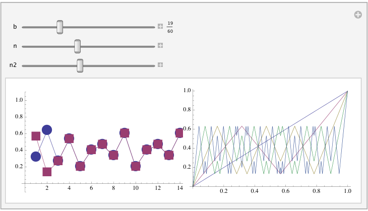
For each Galois conjugate of , there is an embedding of in . In each such embedding, the postcritical orbits remain bounded: the action of on any point is some composition of functions of the form , which act as contractions, so there is a compact subset that the Galois conjugates of every piece, takes inside itself.
By construction, the orbit of the critical points under is also bounded, since is a map of an interval to itself.
For any fixed bound , there are only a finite number of algebraic integers of satisfying the bound , since in the embedding into the product of real embeddings and a selection of one from each pair of complex conjugate embeddings, the algebraic integers in form a lattice. The postcritical set is contained in such a set, so it is finite. ∎
This phenomenon is closely related to why decimal representations of rational numbers are eventually periodic. There is a theory of -expansions, similar to decimal expansions but with a real number; when is Pisot, the digits of the expansion of any element of are eventually periodic (by an almost identical proof). This kind of argument appears in [2], [7], and [14].
The details of construction of above are not important. Any -expander whose critical points are in will do. As long as , there are infinitely many. To make the proof work as phrased, rescale the unit interval to clear all denominators, so that all critical points become algebraic integers in .
Even in the case that is an integer less than , this gives countably many different examples provided . For instance, figure 5 shows the critical point orbits when , and the critical points are chosen as and . On the fourth iterate, they settle into a single periodic orbit of period 4. There is a unique cubic polynomial, up to affine conjugacy, having the same order structure for the postcritical orbits, with entropy .
In general, there is a non-empty convex -dimensional space of -uniform-expanders for every . If is Pisot, then postcritically finite examples are dense in this set.
There are many Pisot numbers: for any real algebraic number , it is easy to see that there are infinitely many Pisot numbers in : the intersection of the lattice of algebraic integers with a cylinder centered around any line corresponding to an embedding of in consists of Pisot numbers, except for those in a closed ball containing the origin. However, in the geometric sense, Pisot numbers are rare: in [13], Salem proved that the set of Pisot numbers is a countable closed subset of , making use of a theorem of Pisot that a real number is Pisot if and only if sequence of minimum differences of from the nearest integer is square-summable. The golden ratio is the smallest accumulation point of Pisot numbers, and the plastic number , a root of is the smallest Pisot number.
It is elementary and well-known that postcritically finite maps are dense among uniform expanders, but the construction above raises a question that does not seem obvious for :
Question 2.2.
For fixed , is there a dense set of numbers for which the set of postcritically finite maps is dense among -uniform expanders? For which are there infinitely many non-affinely equivalent postcritically finite maps? For which are postcritically finite maps dense?
One way to get infinite families of postcritically finite maps with the same is to take dynamical extensions of maps with fewer critical points (c.f. section 10), taking care only to introduce new critical points that map to positions whose forward orbit is finite. But this construction cannot work when .
Salem numbers are closely related to Pisot numbers: some people conjecture that the union of Salem numbers and Pisot numbers is a closed subset of . However, the construction that worked for Pisot numbers is inadequate for Salem numbers. The Galois conjugates of the linear pieces of are isometries of for any conjugate on the unit circle. Let be the degree of the Salem number, so for each linear piece of there are Galois conjugate complex isometries, one for each complex place. If we take the product of these isometries over all complex places of we get an action by isometries on , where the first derivative of the action of each linear piece is , where is a unitary transformation. In the unitary group, the orbit is dense on an torus, acting as an irrational rotation of the quotient of the torus by (thus factoring out the complication of the variable sign of . The action of the sequence of linear functions on the -tuple of moduli appears to behave like a random walk in . Sometimes they are periodic, sometimes with fairly large periods, but Brownian motion in dimension bigger than 2 is not recurrent, and a few experiments for indicate that they typically drift slowly toward infinity, and thus are not postcritically finite. However, there could be some reason (opaque to me) why they might not act randomly in the long run, and they could eventually cycle. At least it seems hard to prove any particular example is not postcritically finite.

For example, for the Salem number 1.7220838 satisfying of degree 4, the critical point of the tent map is periodic of period 5. For the Salem number satisfying , the critical point has period 270. Note that its square is also a Salem number, for which the period is .
One of the most famous Salem numbers is the Lehmer constant, defined by the polynomial . The single root outside the unit circle is . This is the smallest known Salem number, and in fact the smallest known Mahler measure for any algebraic integer. (Mahler measure is the product of the absolute value of all Galois conjugates outside the unit circle.) Figure 7 is a diagram of the first 200,000 elements of the critical point in , projected from to the quadruple of radii in the complex factors, and from there a projection into 3 dimensions. The map is postcritically finite if and only if the path closes. Its values are always algebraic integers, so if it comes sufficiently close to the start it’s fairly likely to close. The quadruple of radii determines a 4-torus in , with the current lattice point a bounded distance from that torus. When the radii are on the order of 200, as in this case, this bounded neighborhood has volume on the order of , with roughly lattice points, so the chances of looping appear remote unless the path wanders close to the origin, where the tori are smaller. For comparison, the variance of a random walk with stepsize 1 in equals the number of steps, so for a random walk of length 200,000, the standard deviation is ; projected from 8 dimensions to 3, the standard deviation would be , in line with the picture. An experiment with a selection of small Salem numbers of moderate degree showed similar results, with none of them exhibiting a cycle within iterates.
This discussion is related to the ideas surrounding the -transformation given by , where . The number is a beta number if has finite orbit under . In [14], Klaus Schmidt showed that every Pisot number is a beta number (proved independently in [2]). In [4], David Boyd proved that if is a Salem number of degree , then it is a beta number. In [5], David Boyd presents heuristic arguments based on random walks that almost every Salem number of degree should be beta. Thanks to Doug Lind for bringing this to my attention.
3. Constructing interval maps: First Steps
For a Perron number that is not Pisot, the situation is much more delicate. To develop a strategy, first we’ll discuss incidence matrices. There are two reasonable versions for an incidence matrix that are transposes of each other. We will use the version whose columns each represent the image of a subinterval of the domain, and whose rows represent a subinterval in the range, so that each entry counts how many times the subinterval that indexes its column crosses the subinterval that indexes its row.
Suppose the unit interval is subdivided into subintervals (in order). Let be the vertex set. Every function that takes adjacent vertices to distinct vertices extends to a postcritically finite piecewise linear map. In this way, a large but finite and specialized set of matrices can be realized as incidence matrices. Incidence matrices are easy to recognize. Each column consists of a consecutive sequence of ’s, and is otherwise . There is a matching between the ends of the blocks of consecutive ’s in adjacent columns, with every column except the first and last having one end of the block of ’s matched to the left and the other end of the block of ’s matched to the right.
Here is a generalization of this concept. Consider a map with finitely many critical points such that and of the critical set is contained in , that is, contains all critical values. Under these conditions, an extended incidence matrix is still defined for , whose entries count how many times crosses interval .
Proposition 3.1.
An non-negative integer matrix is an extended incidence matrix if and only if
- (1)
The nonzero entries in each column form a consecutive block, and
- (2)
There is a map such that in column , the entries in rows greater than and not greater than , and no other entries, are odd.
Proof.
The necessity of the conditions is easy. The map represents the map restricted to . The image of any interval is necessarily the union of a consecutive block of intervals. The subinterval between the images of the first and last endpoints, (which could be a degenerate interval) is traversed an odd number of times, and the rest of the image is traversed an even number of times.
Sufficiency of the conditions is also easy. To map , start from , go to the lowest vertex in the image, zigzag across the lowest interval until its degree is used up, then the next lowest, etc. until you get to , at which point proceed to the highest vertex in the image and work back. ∎
Note: Sufficiency can also be reduced to the familiar condition that a graph admits a Hamiltonian path from vertex to vertex if and only if it is connected and either and all vertices have even valence, or and have odd valence and all other vertices have even valence. For each , apply this to the graph that has edges connecting to . The entire map is really a Hamiltonian path in the graphs connected in a chain by joining vertex of to that of , followed by the natural projection to .
Proposition 3.2.
The topological entropy of any map with extended incidence matrix is the log of the largest positive eigenvalue of .
Proof.
The total variation of is a positive linear combination of matrix entries of (if all intervals have equal length, it is their sum). By 1.1, is the exponent of growth of total variation, so this equals the log of the largest positive eigenvalue of . ∎
Suppose we are given a (strict) Perron number . Our strategy is to first construct a strictly positive extended incidence matrix that has positive eigenvalue , for a large power of . We will promote this to an example with entropy by implanting it as the return map replacing a periodic cycle of a map with entropy less than .
Afterwards, we will deal with additional issues involving questions of mixing and weak Perron numbers.
Given , let be the ring of algebraic integers in the field , and let be the real vector space . Another way to think of it is that is the product of the real and complex places of , that is, the product of a copy of for each real root of the minimal polynomial for and a copy of for each pair of complex conjugate roots. The ring operations of extend continuously to , but division is discontinuous where the projection to any of the places is 0. Yet another way to think of is in terms of the companion matrix for the minimal polynomial of . We can identify with the set of all polynomials in with rational coefficients, and with the vector space on which the companion matrix acts. The real and complex places of correspond to the minimal invariant subspaces of . When is factored into polynomials that are irreducible over , the terms are linear and positive quadratic; the subspaces are in one-to-one correspondence with these factors.
We are assuming that is a Perron number, so for multiplication of by , the -eigenvector is dominant. If we consider the convex cone consisting of all points where the projection to the eigenspace is larger than the projection to any of the other invariant subspaces, then is contained in the interior of except at the origin.
Proposition 3.3.
There is a rational polyhedral convex cone contained in and containing .
Proof.
It is easiest to think of this projectively, in . The projective image of is a convex set (specifically, a product of intervals and disks), with the image of contained in its interior. Since rational points are dense in , we can readily find a set of rational points in the interior of whose convex hull contains ). This gives us the desired rational polyhedral convex cone. ∎
Let be the additive semigroup .
Proposition 3.4.
is finitely generated as a semigroup.
Proof.
This is a standard fact. Here’s how to see it using elementary topology: We can complete by adding on the set of projective limits . The completion is compact. It’s easy to see that the set of closures of the ideals for form a basis for this topology. By compactness, the cover by basis elements has a finite subcover . For any such cover, the set form a generating set: given any element, write it as , and continue until the remainder term is 0. ∎
Proof of Converse Perron-Frobenius 1.4.
Equipped with this picture, it is now easy to prove the converse Perron-Frobenius theorem of Lind. Consider the free abelian group on the set of semigroup generators. The positive semigroup in maps surjectively to . Call this map . We can lift the action of multiplication by to an endomorphism of the positive semigroup, by sending each generator to an arbitrary element of . In coordinate form, this is described by a non-negative integer matrix. In , projection to the -space is a dual eigenvector, that is, a linear functional multiplied by under the transformation. It is strictly positive on . Therefore, the pullback of this function is a strictly positive -eigenvector of the transpose matrix, proving Lind’s theorem. ∎
Note that the minimum size of a generating set might be much larger than the dimension of . For instance, if is a quadratic algebraic integer, is the plane, and could be bounded by any pair of rational rays that make slightly less than a angle to the eigenvector. Minimal generating sets can be determined using continued fraction expansions of the slopes; they can be arbitrarily large.
As we shall presently see, it can happen in higher dimensions that the minimum size of a generating set for can be very large no matter how we choose a semigroup on which multiplication by acts as an endomorphism.
4. Second Step: Constructing a map for
Now we need to address the special requirements for an incidence matrix for a map having a finite invariant set as the set of critical values. Given any Perron number of degree , we will construct such a matrix for some power, probably large, of . From the previous section, 3, we assume we have a set of semigroup generators for a semigroup in invariant under multiplication by .
Choose a finite sequence of generators, including each generator at least once, such that the partial sums of the sequence contain all mod 2 congruence classes, that is, the partial sums map surjectively to . If necessary, adjoin additional elements to the sequence so that the sum of the entire sequence, mod 2, is 0.
The action of (by multiplication) on the projective completion of has a unique attracting fixed point. For any , the closure of contains the fixed point, so there is some power such that .
Now mark off an interval of length into segments whose lengths are given by the chosen sequence of generators (in the embedding of in where goes to ). We’ll construct a -expander map by induction, going from left to right, starting with . There is some point in this subdivision that has the same value mod as . Since can be expressed as plus a sum of generators, it can also be expressed as plus a sum of generators. Since is in and congruent to zero mod 2, it is divisible by 2 in : it can be expressed as where . We can write as a linear combination of generators with even coefficients, so we can write as a strictly positive sum of generators, where each generator between and occurs an odd number of times, and each other generator occurs an even number of times.
We can continue in exactly the same way for times each of the points in the subdivision. We first pick where each point goes based on the congruence class of mod 2, then express the difference as an even and strictly positive linear combination of all generators in the sequence. Finally we end with going to either or , as we choose. The incidence matrix satisfies the conditions of 3.1, so we have constructed a uniform expander.
5. Powers and Roots: Completion of proof of Theorem 1.2
Given a Perron number , we’ll construct a map of to itself that is a uniform expander, because the construction is a little nicer for . From the preceding section, for some we construct a uniform expanding map of an interval that takes each endpoint to itself. Let be any rotation of the circle of order . The circle can be subdivided into intervals that are cyclically permuted by the rotation. Define a metric on the circle so that in this cyclic order, the intervals have length . Now define by mapping each of the first intervals affinely to the next, and mapping the last interval to the first using with affine adjustments in the domain and range to send the last interval exactly to the first. Since the first interval has length times the last, with this affine adjustment also expands uniformly by .
In the case of the circle, we can easily modify the construction of to make the incidence matrix mixing: this will happen if we change any small piece of to stray into a neighboring interval and back, when it gets to the upper endpoint. If the rotation is chosen as a rotation by and if the first generator is chosen to be a ”small” element in , these intervals are small, and straying is probably possible with ease, but in any case, by taking to be a somewhat higher power, it can be readily guaranteed.

In the case of the unit interval, we need a substitute for a rotation of the circle. For this, we can use the well-known period-doubling cascade for quadratic self-maps of an interval (see figure 9 for an illustrative example). In this period-doubling family, there is a quadratic map with entropy 0 in which the critical point has period . We can blow up the forward and backward orbit of the critical point, replacing each point in the orbit by a small interval of any length such that the set of lengths is summable. Extend the map to these intervals by affine homeomorphisms, with the exception of the interval for the critical point; for that, we can use any affine map that takes both endpoints to 0.
Since the entropy of the quadratic map is 0, the number of critical points of grows subexponentially in , so if we assign length to each interval for a point that is critical for but not for , the set of lengths is summable. After blowing up the full orbit of the critical point in this way, we can define a pseudo-metric on the interval where the length of an interval is the measure of its intersection with the blown-up orbit; everything else collapses to measure 0.
By the preceding section, we can find an of the form that maps the unit interval to itself, taking both endpoints to . Implant this, using affine adjustments in the domain and the range, for the map from the interval for the critical point of to its image. The image of the critical interval has length since the original critical point had period , so the implanted map is a uniform -expander.
We now have a map which is a local homeomorphism with Radon derivative in the complement of the critical interval, where it is a uniform -expander. Therefore, the entire map is a piecewise-linear uniform -expander, with entropy . This completes the proof of theorem 1.2 for strong Perron numbers.
Now we’ll address weak Perron numbers.
Proposition 5.1.
A positive real number is a weak Perron number if and only if some power of is a [strong] Perron number.
Proof.
In one direction this is pretty obvious: the th roots of any algebraic integer are algebraic integers, and their ratios to each other are th roots of unity. Thus the positive real th root of a Perron number is a weak Perron number.
In the other direction, suppose is a weak Perron number. Let be the set of Galois conjugates of with absolute value , and let be their product. This product is a real number equal to . The Galois conjugates of are products of Galois conjugates of ; for any subset of conjugates of this cardinality other than , the product is strictly smaller, so is a Perron number. Since , the other elements of also satisfy this equation, so their ratio to is a root of unity. ∎
Now given a weak Perron , we first find a power so that is a Perron number. In the family of degree 2 uniform expanders, functions with periodic critical point are dense, and functions with critical point having period a multiple of are also dense. Choose such a function whose entropy is less than , where the critical point has period a sufficiently high multiple of . Blow up the full (backwards and forward) orbit of the critical point, and implant a map of the form , as constructed in the preceding section 4, in the interval replacing the critical point. Since the growth rate of critical points for powers of is less than the growth rate of powers of , we can construct a metric just as before that is uniformly expanded by .
Note that the -uniform expanders we have constructed are very far from mixing. This is of course impossible if is only a weak Perron number, by the Perron-Frobenius theorem, but for a Perron number it is tempting to try to generalize the straying technique that worked earlier.
There are two difficulties. The first is an essential problem:
Proposition 5.2.
For any self-map of the interval with entropy in the interval , there are two disjoint subintervals that are interchanged by the map, and in particular, is not mixing.
Proof.
For a map , let be the set of points that have more than one preimage. Note that and also ; in fact, . Let , and . Then is mapped into itself, and has the same entropy as .
∎
In particular, they never mix. By induction, if the entropy is less than , there are disjoint intervals cyclically permuted by the map.
The second problem is that the piecewise-linear map we constructed above has coefficients in (either because the formulas from kneading theory for the infinite sums of intervals are rational functions of , or because they are determined by linear functions with coefficients in ), but it is not obvious how to get coordinates to be in . Maybe it’s possible to analyze and control the algebra, but if so it’s beyond the scope of this paper.
6. Maps of Asterisks
Selfmaps of graphs, including in particular Hubbard trees, give another interesting collection of postcritically finite maps of graphs. For use later in constructing automorphisms of free groups, we will look at a special case, the asterisks . An -pointed asterisk is the cone on a set of points, which we’ll refer to as the tips of the asterisk.
Theorem 6.1.
For every Perron number there is a postcritically finite uniform expanding self-map of some asterisk such that
- •
fixes the center vertex, and
- •
each edge maps to an edge-path in a way that every edge is the first element of the image edge-path of some edge
- •
the incidence matrix for is mixing.
A map is topologically transitive if there are dense [forward] orbits under .
Remark 6.2.
Any expanding self-map of a tree can be promoted to a self-map of a Hubbard tree by adding extra information as to a planar embedding, and choosing a branched covering map for the planar neighborhood of each vertex that acts on its link in the given way. Each such promotion is the Hubbard tree for a unique polynomial up to affine automorphism.
Proof.
This is similar to the proof for self-maps of the interval. In principal it is easier because there is no order information to worry about, but we will use a very similar method.
An incidence matrix for a self-map of an asterisk of the given form is a non-negative integer matrix that has exactly one odd entry in each row and each column. Given any such matrix, we can construct a corresponding self-map of an asterisk by permuting the tips according to the matrix mod 2, which is a permutation matrix, and running each edge out and back various edges to generate the even part of the matrix.
As before, find a subsemigroup of that excludes 0 and is invariant under multiplication by .
Let be a finite set of generators for that maps surjectively to . Let .
Let be an integer such that is congruent to 0 mod 2, and for each , is contained in .
Now make an asterisk whose points are indexed by . Map the edge to point homeomorphically to the edge to point when .
The final set of tips will map to tips . For each , is congruent to 0 mod , and so can be expressed as a strictly positive even linear combination of .
Use these linear combinations to construct an asterisk map. Each edge to the first set of tips maps homeomorphically to a new edge for the first iterates. On the th iterate, it maps to a path that makes at least one round trip to all the first layer points as well as one second layer point, finally ending back where it started. We can easily arrange the order of traversal so that every edge is represented in the first segment of one of these edge paths.
If the asterisk is given a metric where edge has length equal to the value of in the standard embedding of in where is the Perron number, this map is a -uniform expander. It is mixing: by the th iterate, the image of an edge with index contains all generators of the form ; by the th iterate, the image of an edge contains all generators of the form and . After iterates, the edge maps surjectively to the entire asterisk. ∎
This construction was intended to avoid the need for complicated conditions and bookkeeping. It’s clear that a more careful construction could produce suitable asterisk maps for a typical Perron number that are much smaller (but still might be quite large).
7. Entropy in bounded degree
The constructions for maps of given entropy have been very uneconomical with the complexity of the maps. First, there is a potentially dramatic (but sometimes unavoidable) blowup in going from a Perron number to a finite set of generators for a subsemigroup of algebraic integers invariant by multiplication by . Even then, there is another possibly large blowup in finding a power of such that is sufficiently deep inside to guarantee an easy construction of a suitable incidence matrix. In other words: unlike Pisot numbers, a typical Perron number is probably unlikely to be the growth constant for a typical postcritically finite map of an interval to itself.


In some sense, expansion constants for bounded degree systems are almost Pisot: most of their Galois conjugates don’t seem to wander very far outside the unit circle. Figure 1 illustrates this point: most of the Galois conjugates of for postcritically finite quadratic maps are in or near the unit circle. Since their minimal polynomials have constant term or , the inside and outside roots are approximately balanced. If they don’t wander outside the circle, they can’t wander very far inside the circle, and most roots are near the unit circle. In contrast, figure 2 illustrates that Perron numbers less than can have roots spread in the disk of their radius.
To get some understanding of what’s going on, we’ll translate questions about the distribution of roots into questions about dynamics of a semigroup of affine maps, elaborating on the point of view taken in the discussion of Pisot numbers in section 2. We’ll consider the sets of piecewise linear uniform expander functions that take onto , where is the number of intervals on which the function is linear and determines the sequence of slopes. is the sequence of slopes in subintervals through . The constant terms for the linear function in the first and last interval are determined by the condition that , implying that if and when , with a similar equation for the last interval. In all other subintervals, the constant term is a free variable subject to linear inequalities. That is, the th critical point , determined by , must be inside the unit interval, so we have the inequalities
Now for any other field embedding in , we can look at the collection of image functions . Since the choice of which to apply is determined by inequalities, we will look at the product action. Define to act on by where is a linear piece that applies to . In the ambiguous case where is one of the critical points, this definition is discontinuous, so we will look at both images, which are the limit from the left and the limit from the right.
Define the boundedness set to be the set of such that the its orbit stays bounded. If is postcritically finite, then the critical points in particular have bounded orbits, so in addition the full orbit of the critical points (under taking inverse images as well as forward images) are bounded. Define the limit set to be the smallest closed set containing all -limit sets for .
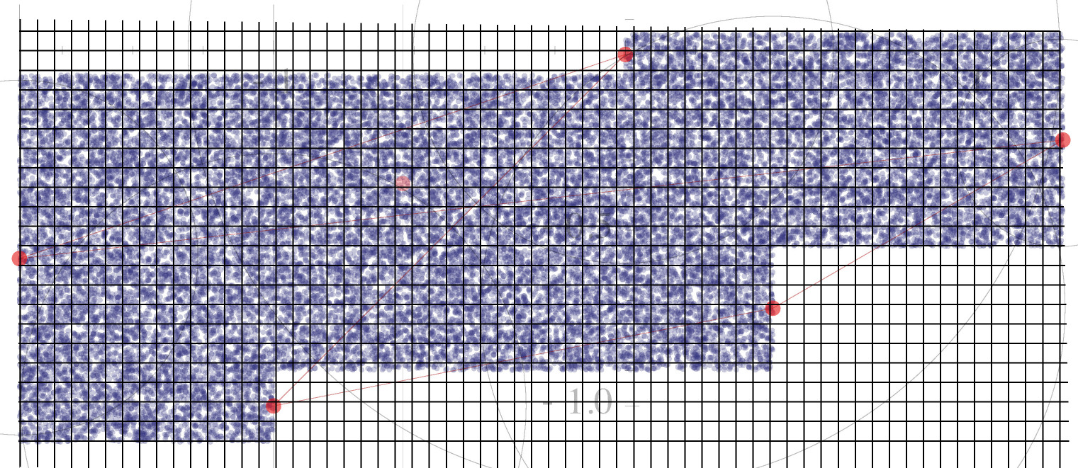
There are three qualitatively different cases, depending on whether is less than 1, equal to 1, or greater than 1.
In the first case that , every orbit remains bounded in the direction, since the map is the composition of a sequence of contractions. Everything outside a certain radius is contracted, so the boundedness locus is compact. Some special examples of this are illustrated in figures 10, 11 and 12.
The second case, when , seems hardest to understand, since the act as isometries. Perhaps the limit set in these cases is all of .
In the third case, when , the maps are expansions, so there is a radius such that everything outside the disk of radius centered at the origin escapes to . Given , the only such that has second coordinate inside are inside a disk of radius about the preimage of 0. Starting far along in the sequence of iterates and working backwards to the beginning, we find a sequence of disks shrinking geometrically by the factor that contain all bounded orbits. In the end, there’s a unique point such that remains bounded. The point can also be expressed as the sum of a power series in with bounded coefficients that depend on the and the kneading data for , matching with formulas from [9].
Proposition 7.1.
If is postcritically finite and if , then depends continuously on .
Proof.
When is postcritically finite, the preperiodicity of at any critical point is equivalent to an identity among compositions of the . Therefore satisfies the same identity when applied to , therefore its orbit is bounded so .
Since is the sum of a geometrically convergent series, the value depends continuously on the coefficients. The coefficients change continuously except where is a precritical point; but the limits from the two sides coincide at precritical points, since they coincide for critical points. Therefore is continuous. ∎
When is not postcritically finite, might not be continuous; there could well be different limits from the left and from the right at critical points, and therefore at precritical points: the natural domain for in general is a Cantor set obtained by cutting the interval at the countable dense set of precritical points. For example, if is transcendental, then could send it to any other transcendental number, and it’s obvious that generically would not be continuous.
This phenomenon points to the inadequacy of considering only the algebraic properties of when our real goal is to control the geometry. Here is a formulation of the appropriate condition, in a slightly bigger context:
Definition 7.2.
Suppose , is a vector space and that has the form
when , where is an expanding map and the is a constant vector. Then is a friendly extension of if there is a continuous map such that the orbit of is bounded.

Since postcritically finite systems are dense in , there are many postcritically finite examples, and many have Galois conjugates of outside the unit circle. Since boundedness depends continuously on the kneading data, the coefficient and the constant terms , we can pass to limits of postcritically finite systems; if we take a convergent sequence of postcritically finite systems having a convergent sequence of friendly extensions, then the limit is also a friendly extension.
In the case , these correspond to the kneading roots which were collected in figure 1. Note that even for a for which is postcritically finite, it is a limit of of much higher degree for which is also postcritically finite; in fact, it is a limit of cases where the critical point is periodic. The minimal polynomials for these nearby polynomials can be of much higher degree, so there can be many more friendly extensions than just the ones associated with the roots of the minimal polynomial for . Figure 13 is a 3-dimensional figure of friendly extensions, where the vertical axis is the direction, and the horizontal direction is ; the plotted points outside the unit cylinder are expansion factors for friendly extensions.
Figure 14 is a very thin slice of the set depicted in figure 13, halfway up and of thickness . A movie made from frames of this thickness, at 30 frames per second, would last a year. This slab is thin enough to freeze the motion of 7 isolated friendly parameters, which you can see around the periphery. One of the 7, at position 1.5, is the original controlling expansion constant . Closer to the unit circle, the friendly parameters are packed closer together, and they move so quickly that they blur together into a big cloud.

Remark 7.3.
The “set of friends” changes continuously, regarded as an atomic measure on the parameter space for candidate systems, in the weak topology.
8. Train Tracks
We have defined a train track map of a graph to be a map such that each edge is mapped by a local embedding under all iterates; now we’ll define a train track structure:
Definition 8.1.
A train track structure for a graph is a collection of 2-element subsets of the link of each vertex, called the set of legal turns.
The mental image is that of a railroad switch, or more generally a switchyard, where for each incoming direction there is a set of possible outgoing directions where trains can be diverted without reversing course. A path on is legal if it is a local embedding, and at each vertex it takes a legal turn.
In describing edge paths, we must first choose an orientation for each edge. We use the convention that a lower case letter denotes the forward direction on the edge, and the corresponding capital letter to denote the backward direction on the edge. This convention also applies to generators of groups (which we can think of as edges in a cell complex having the given group as its fundamental group).
A map preserves if maps every -legal path to a -legal path. It follows that is a train track map: since the forward images of edges must always be legal paths, in particular they are mapped by local embeddings.
For any train track map , there is always at least one train track structure that preserves. The minimal invariant train track structure allows turns only if they are ever taken by the forward image of some edge of the graph. The maximal invariant train track structure allows all turns that are never folded by iterates of , that is, it allows any turn that is always mapped to be locally embedded.
There is an interesting special case of train track structure for a bouquet of circles: the positive train track structure, where the legal paths correspond to paths that are positive words in the generators of the free group. These paths follow a consistent orientation along the circles. More generally, a train track structure is orientable if there is no legal path that crosses an edge twice in opposite directions; orientability holds if an orientation of the edges can be chosen so that all legal paths maintain a consistent direction (but the converse need not hold).
An oriented train track on a graph defines a convex cone in . For an automorphism that preserves such a structure, takes to or to . Therefore, has an eigenvector inside . Just as in the Perron-Frobenius theorem, an eigenvector strictly inside has the largest eigenvalue, and in any case, there is an eigenvector in the cone (possibly on its boundary) whose eigenvalue is largest. This eigenvalue is the same as the expansion constant for , since the incidence matrix for is the matrix for acting on (simplicial) 1-chains of . As an eigenvector for an element of , such an eigenvalue is always an algebraic unit.
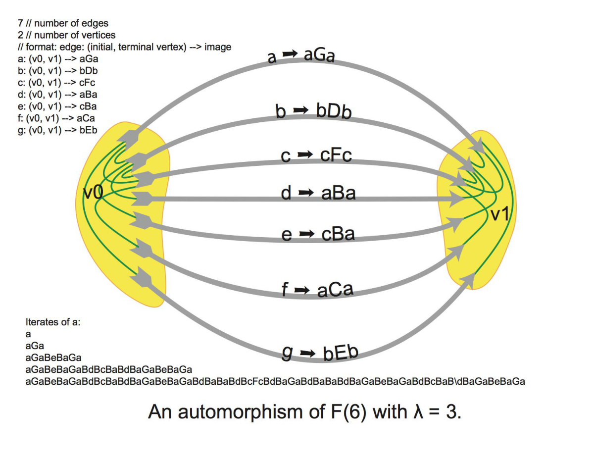
As illustrated by the example of figure 15, the expansion constant for a train track map need not be a unit: the figure describes a map with expansion constant 3.
To check that it is an automorphism, first write down the images of the generators and collapse the edge to a point (thus striking out all ’s):
| (1) | ||||
| (2) | ||||
| (3) | ||||
| (4) | ||||
| (5) | ||||
| (6) |
Every surjective selfmap of a free group is an automorphism, so it’s enough to check that all 6 generators are in the image. We get from , and given we get from . Given and , we get from the image of and from the image of . Given these four generators we get the remaining two, from the image of and from the image of . Therefore, is a self-homotopy-equivalence of the graph, so it gives a train track map.
To see that the map preserves the train track structure, first note that every edge maps to a legal path. Now note that the three edges each map to a path starting and ending in the same way, with or respectively. All words only involving these three edges are legal for this train track. The other four edges map to words beginning and ending with or , so it is easy to check that legal turns are mapped to legal turns.
This implies that there is no orientable train track structure invariant by the automorphism up to homotopy. For this particular example, the structure has an anti-orientation, such that every legal path reverses orientation at every vertex.
For , a map with expansion factor can be defined, preserving the same train track:
| (7) | ||||
| (8) | ||||
| (9) | ||||
| (10) | ||||
| (11) | ||||
| (12) | ||||
| (13) |
A sequence of steps identical to that for shows that is a train track map. For completeness, we can define as the identity map of this train track; is also a train track map. There are similar constructions for even expansion factors, but we do not need them.
9. Splitting Hairs
Let be any purely expanding selfmap of a tree. Every tree is bipartite, so we can partition the vertices into to sets and such that there are no edges of with both endpoints in one of the sets.
The map may not respect this partition; if not, let be the barycentric subdivision of , with one new vertex in the middle of each edge of . For each edge of the original , choose one of the edges in its image, and adjust so that . The new map still has a non-negative incidence matrix. Any positive linear function that is an eigenvector for its transpose pulls back to a linear function that is an eigenvector for the transpose of the incidence matrix of the original , so the eigenvalues are the same. Therefore, there are positions for the new vertices so all vertices of are mapped (by the original ) to vertices of . The graph has a bipartite partition, where consists of original vertices and consists of new vertices, where each partition element is invariant by .
Given any graph and an integer , define a new graph to be obtained by replacing each edge of with edges having its same pair of endpoints. For each edge , label the new edges with subscripts .
When has a bipartite structure , define a train track structure on using the prototype of figure 15: that is, a path is legal if and only if the sequence of subscripts defines a legal path in the prototype.
When is a map of to itself that preserves the partition elements and maps each edge to an edge-path of length at least one, define
using the prototypes defined in the preceding section 8. That is, for an edge of , if has combinatorial length , lift to the map by applying the sequence of subscripts to the sequence of edges .
Note that the themselves are defined by this process, starting with the self-maps of the unit interval that fold it over itself an odd number of times.
Proposition 9.1.
For any bipartite structure on a graph and any map that preserves the partition elements and maps each edge to an edge-path of length at least one, is a train track map.
Proof.
Notice that in the prototype train track, every legal turn has at least one of its ends among the edges . Any turns among these three edges are legal, and every preserves their beginnings and end. Every with maps beginnings and ends in the same way, so a turn between edges whose combinatorial image length is more than 1 maps to a legal turn. Similarly, a legal turn between edges one or both of which have combinatorial image length 1 maps to a legal turn. ∎
Proposition 9.2.
If is a tree with bipartite structure , and if is self-map such that
- •
f preserves and , and
- •
f is a local embedding on each edge, and
- •
the map , that is, goes to the first element of its image edgepath, is a permutation
- •
the map if has length more than 1, and otherwise, is also a permutation
then is a homotopy equivalence.
Proof.
The set of edges with subscript forms a spanning tree for . If we collapse the spanning tree to a point, we obtain a bouquet of circles, so the remaining edges give a free set of generators for the fundamental group.
Pick a basepoint on the graph . As an edge path, the generator corresponding to is obtained by prefixing by the subscript path from to its first vertex, and appending the path from its end vertex back to , then striking out all ’s and ’s.
As before, we just need to show that all generators are in the image of . Consider the 6 generators lying over any particular edge of . Let be the first edge in the edgepath . We will follow the same outline that showed is a homotopy equivalence. The image of under is which becomes after the collapse. Applying this to all edges of , we obtain all generators in the image. Modulo the generators, from we get all generators of the form . Since is a permutation, this gives all subscript generators. From modulo the generators, we get the generators. Continue in the same sequence that was used to show is surjective: modulo previous generators, each edge has a payload generator in the first or second slot of its image, so we get all generators. ∎
Given any Perron number , we can now apply proposition 9.2 to the asterisk map constructed by theorem 6.1, where we take to consist of the center vertex and to consist of all the tips. We obtain a train track map . The maps were constructed so that every edge occurs as the first segment of some image edge-path. The same edge occurs as the second segment, if the path has length more than 1, so the maps and are both permutations. Therefore, is train track homotopy equivalence of which uniformly expands with expansion factor .
The maps are mixing when , from which it follows that is mixing.
If is a weak Perron number, let be the least integer such that is a Perron number. Make an asterisk from copies of an asterisk for , and map it to itself by permuting the factors except for the final map, which is a copy of . From this asterisk map , we obtain a train track automorphism with expansion constant . This completes the proof of theorem 1.6.
10. Dynamic Extensions
If is a continuous map, then an extension of is a space with a continuous surjective map and a semiconjugacy of to , that is, it satisfies .
The hair-splitting construction of section 9 is a special case, which we’ll call a graph extension, where and are graphs and edges of are mapped to non-trivial edge-paths of . If is a -uniform expander, then so is . Given two graph extensions and , they have a fiber product , consisting of all pairs of points in and that map to the same point in . We can pick a connected component of the fiber product to obtain a connected graph that is a common extension of both; thus the set of connected graph extensions is a partially ordered set where any two elements have an upper bound (but not necessarily a least upper bound).
It seems natural to ask which uniformly expanding selfmaps of graphs have graph extensions that are train-track self-homotopy-equivalences. It would also be interesting to strengthen the condition, to require that the fundamental group of the extension graph maps surjectively to the fundamental group of the base; in that case, a necessary condition is that itself be a homotopy equivalence, otherwise neither it nor its extension would be surjective on . If necessary, we could also weaken the condition by allowing a subdvision of before taking the extension.
Although proposition 9.2 required that the first and second elements in the edgepaths for are partitions, this condition does not seem essential. One trick would be to modify the formula of 13 to lift , we could use lifts in patterns such as and to adjust the payload edges to be somewhere else along the edgepath, taking care that the payload edges map surjectively, and that they are chosen so that there is an order that will unlock them inductively.
It seems plausible that by a combination of duplicating edges, subdividing edges, and lifting with adjustable payloads, any expanding self-homotopy-equivalence of a graph would have an extension that is a train track map of a graph whose fundamental group maps surjectively to the base. However, it is beyond the scope of the current paper to pursue this.
It would also seem interesting to understand a theory of minimal uniformly expanding maps, ones that cannot be expressed as non-trivial extensions. Perhaps extensions that merely identify vertices should be factored out. This should be related to a theory of finitely generated abelian semigroups that exclude 0 and are invariant by a transformation and which, tensored with , have as dominant eigenvalue. They can be thought of as a positive -modules.
11. bipositive matrices
Definition 11.1.
A pair of real numbers is a conjugate pinching pair if and are algebraic units whose Galois conjugates are contained in the open annulus of inner radius and outer radius . They are a weak conjugate pinching pair if their conjugates are contained in the closed annulus.
Here is an elementary fact:
Proposition 11.2.
A real number is the expansion constant for an element of for some if and only if it is a weak Perron number.
A pair of algebraic units occurs as the pair of expansion constants for and if and only if the pair is a weak conjugate pinching pair.
Proof.
Sufficiency is easy. Given a weak Perron number , the companion matrix for the minimal polynomial for has expansion constant . Given a conjugate pinching pair , take the sum of the companion matrix for a minimal polynomial for with the inverse of a companion matrix for the minimal polynomial for .
Necessity is pretty obvious: must be the maximum absolute value, and the minimum, among all roots of . ∎
Definition 11.3.
An invertible matrix is bipositive with respect to a basis if admits a partition into two parts and such that maps the orthant spanned by to itself, and maps the orthant spanned by to itself.
If either of the two positive matrices associated with a bipositive matrix is mixing, the other is as well, so in this case we also say the bipositive matrix is mixing. Similarly, we will call a bipositive matrix mixing if all sufficiently high powers have all non-zero entries. More geometrically, given a positive matrix, we can make a graph whose vertices are the basis elements and whose edges correspond to nonzero entries. The matrix is primitive if there are edge-paths of every sufficiently long length from each vertex to each others. The set of lengths of edge-paths from one vertex to another is a semigroup, and it is easy to see that its complement is finite if and only if the elements have a common divisor larger than one. It follows that an irreducible positive or bipositive matrix is mixing if and only if every positive power of is ergodic.
Theorem 11.4.
A pair is the pair of positive eigenvalues for an invertible bipositive integral matrix of some dimension if and only if it is a conjugate pinching pair, or a weak conjugate pinching pair such that all conjugates of and of modulus or are or times roots of unity.
Remark 11.5.
The clause about roots of unity addresses the issue that although all Galois conjugates of a weak Perron number that have maximum modulus are at angles that are roots of unity, the Galois conjugates of minimum modulus need not be.
For instance, if is the plastic number which is a root of , its other two conjugates have modulus , so is a weak conjugate pinching pair. However, the two complex Galois conjugates of are at angles that are irrational multiples of . Therefore is not the pair of expansion constants for any bipositive matrix.
Proof.
We will first establish the theorem in the case is a [strict] conjugate pinching pair.
First, let have eigenvectors and of eigenvalues and . By restricting to the smallest rationally defined subspace of containing and , we may assume that all other characteristic roots of are in the interior of the annulus . Let be the real subspace spanned by and , and be the projection that commutes with .
Let be the line through the origin of slope in the -plane. The linear transformation multiplies slopes by , so has slope . Let be the reflection of L in the -axis; thus is the reflection of .
Choose a set of lattice points such that lies in the interior of the first quadrant of the -plane, generates the lattice as a group, and the convex cone generated by contains the angle between and , except , in its interior. Similarly, choose to be a set of lattice vectors that generate as a group, that are mapped by to the interior of the fourth quadrant, generates as a group, and contains the angle between and .
Let be the semigroup generated by and let be the semigroup generated by .
We claim that for sufficiently large and for any two elements there is a such that
and similarly, for any there is a such that
To see this, we will make use of a basic fact about the semigroups of lattice elements:
Lemma 11.6.
Let be a finite set of elements of the lattice , and let be the convex cone generated by . There is some constant such that any element of the group generated by whose radius ball is contained in is also contained in the semigroup generated by .
Proof.
The convex cone is the set of all non-negative real linear combinations of elements of . If we express an element of as a non-negative real linear combination of elements of and round the coefficients to the nearest integer, we see that is within a bounded distance of some element of .
Let be the set . Express each element of as an integer linear combination . Let be the maximum, among these linear combinations, of the norm of the set of negative coefficients, and set .
Now for any element such that , there are elements and such that .
∎
Now for large, the image in projective space of is close to the image of the eigenspace . The images march in the direction of the axis, projectively converging to the eigenspace, with the slope in the -plane of the line from to decreasing by a factor of at each iterate. If is suitably large, at least one of these iterates is the center of a large ball captured in the interior of the cone and so, by the lemma, in the semigroup .
Now we can describe an irreducible bipositive matrix. Take the free abelian group generated by
We will choose a bipositive map of to itself that commutes with evaluation in . The generators pass off from one to the next until . Choose a cyclic permutation of of and a cyclic permutation of . For each choose an expression where is an element of , and similarly for express , with . Use this to give the final links in the chain, to define .
The matrix for the linear transformation can be expressed as an upper triangular matrix followed by a permutation, hence it is invertible. In block form, the generators are each expressed as another generator plus an element of the semigroup, and vice versa. The inverse has the same form, but with semigroup elements subtracted; reversing the sign of the generators turns the inverse into a positive matrix.
The matrix for is irreducible because of the cyclic permutations: the images of each generator eventually involves each other generator, and (except in the trivial case ) the powers of the matrix are eventually strictly positive. The positive eigenvalue for is , since projection to the axis gives a linear function, positive on the positive orthant for , that is a dual eigenvector of eigenvalue . Similarly, the positive eigenvalue for is .
If is a weak conjugate pinching pair such that all conjugates of or on the circle of maximal or minimal modulus have arguments that are rational multiples of , let be a common multiple of the denominators. Then is a strict conjugate pinching pair; let be a matrix realizing this pair of pinching constants. Take the direct sum of copies of the underlying vector space, permute them cyclically, with return map . This is a bipositive matrix realizing .
For the converse: consider any bipositive matrix with positive eigenvalue and positive eigenvalue for where one or both are not the unique characteristic roots of maximum modulus say there are roots of modulus . Then there is a -dimensional subspace with a metric where acts as a similarity, expanding by a factor of . Hence, the projective image of this subspace is mapped isometrically. Its intersection with the image of the positive orthant is a polyhedron mapped isometrically to itself; hence, its vertices are permuted. It follows that all characteristic roots of modulus have the form of times an th root of unity. ∎
A simple example of the construction for a weak conjugate pinching pair is the Fibonacci transformation and , with eigenvalues , the golden ratio and . The square of this transformation is and , which is bipositive: its inverse maps the second quadrant to itself. This translates into a bipositive map for in dimension 4, that expresses a bipositive linear recurrence for four successive terms of the Fibonacci sequence,
As another example, and ) can be realized by a bipositive transformation in dimension 12.
Question 11.7.
(suggested by Martin Kassabov) Suppose has dominant eigenvalue and has dominant eigenvalue where is a [strict] conjugate pinching pair. Is there a basis for which some power of is bipositive?
Remark 11.8.
Although elementary matrices generate , and together with permutations generate , the semigroup is a very different matter: for , the elementary positive semigroup is not even finitely generated.
To see the gap between the elementary positive semigroup and the full positive semigroup of , let’s focus on the case (The embedding in that fixes all but the first 3 basis elements gives examples, albeit atypical, for arbitrary dimension ).
Let’s look at the action of these semigroups on the basis triangle in . The image of the triangle by a word in the generators gives a sequence of subtriangles of this triangle, where at each step you bisect one of the sides and throw one half away. In particular, each possible proper image is contained in one of six half-triangles of .
Now consider in general positive element of . It maps the tetrahedron spanned by together with the basis elements to a ‘clean’ lattice tetrahedron, that intersects lattice points only at its vertices. This property (clean) characterizes the possible images. Furthermore, any clean triangle in the positive orthant with one vertex at the origin can be extended (in many ways) to a clean tetrahedron: just add any vertex in one of the two lattice planes neighboring the plane containing the triangle
But there are many clean triangles; in fact, the set of lattice points in the positive orthant that are primitive (i.e. the 1-simplex from the origin to the point is clean) have density , and given a primitive lattice point , the density of lattice points such that the triangle is clean is . It follows that every line segment contained in can be approximated in the Hausdorff topology by an image of under the positive semigroup of . Many such line segments cross all 3 altitudes of , so a positive element of that maps to a nearby triangle is not in the positive elementary semigroup.
Nonetheless, images of under the positive semigroup of are quite restricted. For instance, it’s easy to see that the centroid of , corresponding to the line , cannot be in the interior of any image of . For any finite collection of triangles not containing the centroid in their interior, most lines through the centroid are not contained in any one of them. Therefore, no finite set of positive images of cover all possible images.
Note that the proof for theorem 11.4 actually gave something stronger. If we have a basis that is partitioned into two parts and , then any elementary transform that replaces an element of by its sum with an element of , or an element of by its sum with an element of is bipositive. The elementary bipositive semigroup [with respect to ] is the semigroup generated by these cross-type elementary transformations, together with permutations that preserve and .
Theorem 11.9.
A pair of real algebraic units is the pair of expansion constants for an elementary bipositive matrix and its inverse if and only if it is a conjugate pinching pair such that all Galois conjugates of or of maximal or minimal modulus have arguments that are roots of unity.
Proof.
From the proof of theorem 11.4, the condition on arguments is an equivalent form of the hypothesis in the case that does not strictly pinch. ∎
12. Tracks, Doubletracks, Zipping and a sketch of the Proof of Theorem 1.8
Continuous maps are often inconvenient for representing homotopy equivalences between graphs, because a self homotopy equivalence cannot be made into a self-homeomorphism of any graph in the homotopy class unless it has finite order up to homotopy.
Continuous maps of graphs can be inconvenient as geometric representatives of group automorphisms of the free group, since they are usually not invertible. As we have seen, it is not easy to see at a glance whether a given map of graphs is a homotopy equivalence. There are algorithms to check, but they can be tedious.
As an alternative, we can represent self-homotopy equivalences by continuous 1-parameter families of graphs. These have the advantage of being reversible. If we restrict to graphs that have no vertices of valence 1, these can be locally described by moving attachment points of edges along paths in the complement of the edge.
A zipping of a train track to a train track is a 1-parameter family of structures that may be thought of as squeezing together legal paths. It’s elementary to see that for any train track map , there is a zipping that yields the homotopy class of : just progressively and locally zip together the identifications that will be made by the map.
A zipping can be translated into a sequence of reversible steps, consisting of a motion of an attachment point of one edge along a legal path on its complement, starting in a direction in its linkgroup. When is zipped to , every bi-infinite -legal path becomes a bi-infinite -legal path. The inverse of a zipping is an unzipping or splitting.
A doubletrack structure for is a pair of train track structures on . A graph equipped with a pair of train track structures is a doubletrack.
A bizipping between doubletracks, is a 1-parameter family of doubletracks that is a zipping of the first train track structure and an unzipping of the second. This yields a train track map of one structure whose inverse is a train track map for the other structure.
Remark 12.1.
It seems likely that invariant foliations could provide a good alternative to train tracks. Bestvina and Handel introduced a concept of train tracks relative to an invariant filtration of a graph, and showed that relative train track maps exist for every outer automorphism of a free group (not just in the irreducible case). Instead, one could look at foliations of finite depth on a manifolds of sufficiently high dimension (as a function of the rank of the free group), with singularities having links based on polyhedra, and satisfying the condition (used to great effect by Novikov) that there are no null-homotopic closed transversals. Such a foliation picks out a class of bi-infinite words in the free group. Bestvina-Handel’s theorem on existence of relative train tracks would appear to translate to the existence of a homeomorphism of some open manifold homotopy-equivalent to a bouquet of circles that preserves such foliation. Pairs of foliations could substitute for doubletracks.
We will not take the detour of trying to develop this point of view here.
We now sketch the proof of theorem 1.8.
Proof.
We will now analyze the [main] case when there are strict inequalities: let be a strictly pinching pair of algebraic units.
From theorems 11.4, let A be a bipositive matrix with positive eigenvectors for and for having eigenvalues and . Let be the invariant projection of the vector space for to the plane spanned by and . The basis is partitioned into two sets, and , with in the first quadrant and in the fourth quadrant. The negations of these two sets give vectors that are mapped into the other two quadrants.
We claim that, for a suitable choice of and , there is a permutation of the basis such that for any the difference is a non-negative linear combination of basis vectors that map to the quadrant neighboring the quadrant of across the axis. (To help with visualization: for most basis elements, will be chosen so that .)
Suppose this claim is true. Let be a graph with a single vertex whose edges correspond to . Let be the homomorphism that maps the loop of an edge labeled by a vector to that vector, and let be the corresponding covering space. ( can be visualized as an embedded graph in the torus , and is lift to a graph in ). Define a doubletrack structure on where a -legal path lifted to has monotone projection to the -axis and a -legal path lifts to have monotone projection to the -axis. The linear transformation maps to a new graph mapped to . Using the claim above, we can construct a bizipping that slides the image edges back to the originals.
∎
References
- [1] L. Alsedà, J. Llibre, and M. Misiurewicz. Combinatorial dynamics and entropy in dimension one, volume 5 of Advanced Series in Nonlinear Dynamics. World Scientific Publishing Co. Inc., River Edge, NJ, second edition, 2000.
- [2] A. Bertrand. Développements en base de Pisot et répartition modulo . C. R. Acad. Sci. Paris Sér. A-B, 285(6):A419–A421, 1977.
- [3] M. Bestvina and M. Handel. Train tracks and automorphisms of free groups. Ann. of Math. (2), 135(1):1–51, 1992.
- [4] D. Boyd. Salem numbers of degree four have periodic expansions. In Théorie des nombres (Quebec, PQ, 1987), pages 57–64. de Gruyter, Berlin, 1989.
- [5] D. Boyd. On the beta expansion for Salem numbers of degree . Math. Comp., 65(214):861–875, 29–31, 1996.
- [6] A. de Carvalho and T. Hall. Unimodal generalized pseudo-Anosov maps. Geometry & Topology, 8:1127–1188, 2004.
- [7] A. O. Gelfond. A common property of number systems. Izv. Akad. Nauk SSSR. Ser. Mat., 23:809–814, 1959.
- [8] D. A. Lind. The entropies of topological Markov shifts and a related class of algebraic integers. Ergodic Theory Dynam. Systems, 4(2):283–300, 1984.
- [9] J. Milnor and W. Thurston. On iterated maps of the interval. In Dynamical systems (College Park, MD, 1986–87), volume 1342 of Lecture Notes in Math., pages 465–563. Springer, Berlin, 1988.
- [10] M. Misiurewicz and W. Szlenk. Entropy of piecewise monotone mappings. In Dynamical systems, Vol. II—Warsaw, pages 299–310. Astérisque, No. 50. Soc. Math. France, Paris, 1977.
- [11] M. Misiurewicz and W. Szlenk. Entropy of piecewise monotone mappings. Studia Math., 67(1):45–63, 1980.
- [12] V. Nekrashevych. Hyperbolic groupoids: definitions and duality, 2011. arXiv:1101.5603v1.
- [13] R. Salem. A remarkable class of algebraic numbers. Proof of a conjecture of Vijayaraghavan. Duke Math. Journal, 11:103–108, 1944.
- [14] K. Schmidt. On periodic expansions of Pisot numbers and Salem numbers. Bull. London Math. Soc., 12(4):269–278, 1980.