Minimizing the Probability of Lifetime Ruin Under Ambiguity AversionThanks: This research is supported by the National Science Foundation under grant DMS-0955463.

The problem of how individuals should invest their wealth in a risky financial market to minimize the probability that they outlive their wealth, also known as the probability of lifetime ruin (this terms was coined by [32]), was analyzed by Young [42]. We mention that Jacka in an earlier work [22] considered a finite-fuel problem of very similar form. Subsequent variants of Young’s work include but not limited to adding borrowing constraints [7], assuming consumption is ratcheted [8], allowing stochastic consumption [9] and stochastic volatility [4]. In all previous works, there is a fixed risky asset model; that is, the investor is certain about the evolution and distribution of the risky asset price. This is, however, not very realistic. There may be good estimates of the price volatility, but drift estimation, as Rogers points out in [34, Section 4.2], is almost impossible; it would require centuries of data to obtain a reliable estimate. Therefore, it is desirable to have a robust investment strategy that can perform well against drift misspecification. For a good introduction of robust decision making theory, see [17].

Although drift estimation is difficult, one would still like to make use of the available data. A natural approach is to extract from the available data a reference model, and penalize other models based on their deviation from the reference model. How hard to penalize depends on how averse the agent is to ambiguity, also called model uncertainty or Knightian uncertainty. Early works incorporating ambiguity aversion into optimization (e.g. [30], [18]) are mostly done via a formal analysis of the corresponding Hamilton-Jacobi-Bellman (HJB) equation. Among those that provide more mathematical rigor, we mention a few that use different approaches. Jaimungal solves a finite horizon irreversible investment problem [24], and a hybrid model of default problem with Sigloch [25] using stochastic control. They work with a scaled entropic penalty in order to get explicit solutions and rely on direct verification. Bordigoni et al. [11] analyze a finite horizon utility maximization problem also by control method, but provide a backward stochastic differential equation (BSDE) characterization instead of an HJB characterization. Their results are generalized to an infinite horizon setting by Hu and Schweizer [20]. Schied [35] and Hernández-Hernández and Schied [19] treat robust utility maximization problems using duality or a combination of duality and control.

In this paper, we provide a complete and rigorous analysis of the robust lifetime ruin problem

using stochastic control, where $\tau_{b}$ and $\tau_{d}$ are the ruin time and death time, respectively, $h^{d}$ is a variant of the entropic penalty function which only measures entropy up to the death time, $\varepsilon$ specifies the penalization strength, $\pi$ runs through a set of investment strategies and $\mathbb{Q}$ runs through a set of possible models representing drift uncertainty. When the hazard rate is zero, we obtain explicit formulas. In the general case, we characterize the value function as the unique classical solution of an associated HJB equation satisfying two boundary conditions, and give feedback forms for the optimal investment and drift distortion. In contrast to the non-robust case or robust utility maximization problem, we show that the value function loses convexity for a class of parameters, which suggests that the Isaacs condition may fail. Same as the non-robust case, we also show that the optimally controlled wealth process never reaches the so-called “safe level”. This is different from the zero-hazard rate case, goes back to the work of Pestien and Sudderth [33] (also see [3]). The goal in the zero-hazard rate case is to reach the safe level (possibly in infinite time) because the individual never dies, whereas the goal when the hazard rate is non-zero is to stay away from the ruin level and to “win” the game by dying. Without a deadline, the optimal strategy is to maximize the ratio of drift to volatility squared. Adding death to the problem changes it tremendously. In particular, we shall see that in terms of the optimal investment strategy, the robustness is only non-trivial then.

Our work extends the discussion in [42] to the robust case. Unlike [24] and [25] where a scaled entropic penalty leads to explicit solutions, our random horizon robust problem, even in the simple Black-Scholes framework, fails to have an explicit solution in general, whether the penalty is scaled or not. Moreover, due to degeneracy and the control space being unbounded, the classical nonlinear elliptic theory by Krylov [28] cannot be applied directly. So we have to resort to the theory of viscosity solutions and then upgrade regularity by bootstrapping. Our work differs from [11], [20], [35], [19] in the methodology. The BSDE characterizations in [11] and [20] only focus on the inner $\mathbb{Q}$-maximization problem and do not describe the optimal investment strategy or the saddle point. The duality approach of [35] requires the infimum and supremum to be exchangeable, which does not hold in our case with certain choice of parameters. The classical duality $\log\mathbb{E}[e^{X}]=\sup_{\mathbb{Q}\in\mathcal{Q}_{abs}}\{\mathbb{E}^{\mathbb{Q}}[X]-h(\mathbb{Q}|\mathbb{P})\}$ between free energy and entropic penalty may look useful at a first glance, but the uncertainty set $\mathcal{Q}_{abs}$ does not preserve the independence between asset price and mortality, and does not leave room for varied confidence levels regarding different model components.¹¹ 1 $\mathcal{Q}_{abs}$ denotes the set of measures that are absolutely continuous with respect to $\mathbb{P}$ and have finite entropy. In addition, we are not using the exact entropic function $h$, but its variant $h^{d}$. Due to time-inconsistency issue, we do not consider uncertainty in hazard rate. It could be an interesting extension to have uncertain Poisson jump rate (see e.g. [29], [31], [12], [10]) and to allow varied positive levels of ambiguity aversion (see e.g. [41], [24]).

For the construction of a viscosity solution to the HJB equation, we use a “comparison + Perron’s method” approach described in [13] instead of the usual route of “dynamic programming principle (DPP) + value function is a viscosity solution + comparison”. The reason is that robust optimization problems resemble stochastic differential games in which nature can be regarded as the second player, and the DPP for games is generally complicated because of measurability issues. One either has to use the Elliott-Kalton formulation where one player uses controls and the other player uses “strategies”, i.e. maps defined on a set of controls satisfying nonanticipitivity (see e.g. [16], [15], [5]), or restrict oneself to strategies of simple form, for example, to what Sîrbu [37] calls elementary strategies. Both ways to get around the measurability issues are not ideal for us. In particular, it is a bit unnatural for us to use the Elliott-Kalton formulation and assume nature is a strategic player against us, because nature has no payoff and is disinterested. It turns out that the classical Perron’s method yields a much simpler and more elegant construction. The only drawback is that regularity now becomes very important, otherwise the constructed solution cannot be related to the value function. Fortunately, we are able to upgrade regularity and carry out a verification theorem. The approach outlined here was first used by Janeček and Sîrbu [26] in a pure stochastic control problem.

Convexity is usually key to upgrading regularity. One challenge introduced by robustness, as we have pointed out, is the loss of convexity of the value function for a class of parameters. In fact, even for non-robust lifetime ruin problems, a priori convexity of the value function is not clear. For example, [9] obtains convexity for a lifetime ruin problem with stochastic consumption by going to a controller-and-stopper problem whose convex dual is related to the original problem through a dimension reduction. We overcome this challenge by working with an equivalent convex problem obtained through the Cole-Hopf transformation. Once we have convexity, it is easy to upgrade to $C^{1}$-regularity using convex analysis and the theory of viscosity solutions. We further upgrade to $C^{2}$-regularity by analyzing a Poisson equation, where we borrow some techniques from [26] and [36]. One may try to prove $C^{2}$-regularity by the regularization method used in [43] and [14], but such an approach requires us to prove the existence of a positive lower bound on $\pi$ that is independent of the regularization on compact intervals away from the safe level, which we find to be difficult to establish.

The rest of the paper is organized as follows. In Section 2, we set up the problem, derive the HJB equation and feedback forms heuristically, and state the main results. Section 3 provides an explicit solution when the hazard rate is zero, which is not only interesting for its own sake, but serves as a useful upper bound in the analysis of the general case. Sections 4 and  5 are devoted to establishing the existence of a classical solution to the HJB equation, with Secitons 4 focusing on Perron’s construction of a viscosity solution, and Section 5 on regularity. In Section 6, we give a verification theorem and the proof of our main results. In order to prove verification theorem, we also show the boundedness and Lipschitz continuity of the optimal investment strategy. Sections 7 collects some additional properties of the optimal investment strategy and the value function. Sections 8 provides numerical results and formulas for small $\varepsilon$-expansion.

Let $\Omega^{M}$ be the space of continuous functions $\omega:[0,\infty)\rightarrow\mathbb{R}$, equipped with the topology of uniform convergence on compact subintervals of $[0,\infty)$. Let $\mathcal{F}^{M}$ be the Borel sigma-algebra on $\Omega^{M}$ and $\mathbb{P}^{M}$ be the Wiener measure on $(\Omega^{M},\mathcal{F}^{M})$. The coordinate map $B_{t}(\omega):=\omega(t)$ is a standard Brownian motion in this space. Here $\mathbb{P}^{M}$ serves as a reference measure which reflects an individual’s belief about the market. Let $N=(N_{t})_{t\geq 0}$ be a Poisson process with rate $\lambda$ defined on another probability space $(\Omega^{d},\mathcal{F}^{d},\mathbb{P}^{d})$. Let $\tau_{d}$ be the first time that the Poisson process jumps, modeling the death time of the individual. $\tau_{d}$ is an exponential random variable with parameter $\lambda$ which is known as the hazard rate in this context. Define

$B$ and $N$ are independent on this space, and remain a Brownian motion and a Poisson process, respectively. Let $\mathbb{F}=(\mathcal{F}_{t})_{t\geq 0}$ be the (raw) filtration generated by the Brownian motion $B$ and $\mathbb{G}=(\mathcal{G}_{t})_{t\geq 0}$ be the filtration generated by $B$ and the process $1_{\{\tau_{d}\leq t\}}$. Assume both $\mathbb{F}$ and $\mathbb{G}$ have been made right continuous. However, we do not complete the filtrations because later on, we would like to include measures that are only locally equivalent to $\mathbb{P}$ as part of our consideration.²² 2 By locally equivalent, we mean equivalent on $\mathcal{G}_{t}$ for all $t\geq 0$. Although the filtrations in our setup is not complete, stochastic integral can still be defined and has all the usual properties. In particular, Itô’s lemma is still valid. See, for example, chapter 1 of [23].

The individual invests in a financial market consists of a risk-free bank account with interest rate $r>0$ and a risky asset whose price $S_{t}$ follows a geometric Brownian motion:

where $\mu>r$ and $\sigma>0$. Let $\boldsymbol{\pi}_{t}$ be the amount that the individual invests in the risky asset at time $t$. Apart from investment, the individual also consumes at a constant rate $c>0$ of her current wealth $w$.³³ 3 To simplify the discussion, we only work with constant consumption rate. But the main techniques can be applied to proportional consumption rate, and more generally, to the case when the consumption rate is a non-negative, Lipschitz continuous function of wealth. Her wealth $W_{t}$ evolves according to the stochastic differential equation (SDE):

An investment strategy $\boldsymbol{\pi}$ is admissible if it is $\mathbb{F}$-progressively measurable and almost surely bounded (uniformly in time).⁴⁴ 4 Almost sure boundedness can be relaxed as long as the best drift distortion in response to each $\boldsymbol{\pi}$ defines an admissible measure $\mathbb{Q}\in\mathscr{Q}$ where $\mathscr{Q}$ is the model uncertainty set to be introduced. Denote by $\mathscr{A}$ the set of all admissible strategies.

Let $\tau_{b}:=\inf\{t\geq 0:W_{t}\leq b\}$ be the first time the individual’s wealth falls to or below a specified ruin level $b$. The individual aims at minimizing the probability that ruin happens before death, i.e. $\tau_{b}<\tau_{d}$, in a robust sense. More precisely, she suspects that the drift of the risky asset may be misspecified. So instead of optimizing under the reference measure $\mathbb{P}$, she considers a set $\mathscr{Q}$ of candidate measures that are locally equivalent to $\mathbb{P}$, and penalizes their deviation from $\mathbb{P}$. Here we assume the individual is only robust against the market model, but not the death time model, nor the independence between them. So elements in $\mathscr{Q}$ should be of the form $\mathbb{Q}^{M}\times\mathbb{P}^{d}$ so that $\tau_{d}$ remains an $exp(\lambda)$ random variable under all candidate measures. Let $h(\mathbb{Q}|\mathbb{P}):=\mathbb{E}^{\mathbb{Q}}[\log\frac{d\mathbb{Q}}{d\mathbb{P}}]$ be the relative entropic function. Denote by $\mathbb{Q}_{t}$ the restriction of a measure $\mathbb{Q}$ to $\mathcal{G}_{t}$. We penalize the deviation from $\mathbb{P}$ using a variant of $h$:

which only measures the relative entropy on $\mathcal{G}_{\tau_{d}}$; that is, the individual does not care about drift uncertainty after death. She faces the following robust optimization problem:

where the subscript $w$ represents conditioning on the event $W_{0}=w$. The parameter $\varepsilon$ measures the individual’s level of ambiguity aversion or preference for robustness. $\varepsilon\downarrow 0$ corresponds to the classical non-robust case since all measures other than $\mathbb{P}$ would give a very negative value, thus not optimal for the inner maximization problem. A larger $\varepsilon$ means the individual is more ambiguity averse, has less faith in the reference model and will consider larger drift distortion. $\varepsilon\rightarrow\infty$ corresponds to the worst-case approach, i.e. the individual has equal belief in all candidate measures and optimize again the worst-case scenario.

We now give the precise definition of the set $\mathscr{Q}$ of candidate measures. A probability measure $\mathbb{Q}\in\mathscr{Q}$ if

for some $\mathbb{F}$-progressively measurable process $\boldsymbol{\theta}$ satisfying $\mathbb{E}[e^{\frac{1}{2}\int_{0}^{t}\boldsymbol{\theta}_{s}^{2}ds}]<\infty$ for all $t\geq 0$, and $\mathbb{E}^{\mathbb{Q}}[\int_{0}^{\infty}e^{-\lambda s}\boldsymbol{\theta}^{2}_{s}ds]<\infty$. Conversely, given any $\mathbb{F}$-progressively measurable process $\boldsymbol{\theta}$ satisfying $\mathbb{E}[e^{\frac{1}{2}\int_{0}^{t}\boldsymbol{\theta}_{s}^{2}ds}]<\infty$ for all $t\geq 0$, we can define a consistent family of measures $\mathbb{Q}_{t}\sim\mathbb{P}_{t}$ on $(\Omega,\mathcal{G}_{t})$ by (2.2). By [38, Lemma 4.2] (also see [21, Proposition 1]), there exists a probability measure $\mathbb{Q}$ on $(\Omega,\mathcal{F})$ such that $\mathbb{Q}|_{\mathcal{G}_{t}}=\mathbb{Q}_{t}$ for all $t\geq 0$.⁵⁵ 5 The existence of such a measure is not guaranteed if the filtration has been completed w.r.t. $\mathbb{P}$. Throughout this paper, we will use boldface greeks $\boldsymbol{\pi},\boldsymbol{\theta}$ to denote controls (as stochastic processes) and plain greeks $\pi,\theta$ to denote the values that the controls can take. Since $\tau_{d}$ is independent of $\mathbb{F}$, the distribution of $\tau_{d}$ is invariant under such change of measure. Under $\mathbb{Q}$, $S_{t}$ has drift $\mu+\sigma\boldsymbol{\theta}_{t}$ and $W_{t}$ has dynamics:

where $B^{\mathbb{Q}}$ is a $\mathbb{Q}$-Brownian motion independent of $\tau_{d}$.

Let $\mathbb{Q}\in\mathscr{Q}$. We have

Substituting the expression for $h^{d}(\mathbb{Q}|\mathbb{P})$ into (2.1) and using the distribution of $\tau_{d}$, we rewrite the value function as:

Denote by $\psi_{0}$ the non-robust value function and by $\mathfrak{p}$ the robust value function when $\lambda=0$, i.e. when the individual never dies. $\psi_{0}$ has the explicit formula (see [42]):

and the optimal investment strategy in feedback form is given by

for $w\in(b,w_{s})$, where

Throughout this paper, $d$ and $R$ will be reserved for the constants defined above. We will also provide an explicit formula for $\mathfrak{p}$ later. For now, we make the simple observation:

where the second inequality holds because $\mathbb{P}\in\mathscr{Q}$ so that

the third inequality holds because ruin before death is no more likely than ruin before infinity, and the last inequality holds because we are optimizing a real probability minus a nonnegative penalty. This means we can treat the robust optimal value as a conservative ruin probability. The penalty term will only cause a small distortion on the ruin probability and will never drive it negative because only measures with small relative entropy are relevant, i.e. have the possibility of being worse than the reference measure.

The definition of $\psi(w;\varepsilon)$ implies it is non-decreasing in $\varepsilon$, since the penalty gets smaller as $\varepsilon$ gets larger. We will suppress the argument $\varepsilon$ throughout the rest of this paper unless we need to emphasize the $\varepsilon$-dependence. The limit as $\varepsilon\downarrow 0$ gives us the non-robust value function $\psi_{0}$. The limit as $\varepsilon\rightarrow\infty$ gives us the worst-case value function:

For the worse-case problem, the optimal investment strategy is not to invest at all since the drift can be arbitrarily unfavorable (negative if one longs and positive if one shorts) without incurring any penalty. The individual can only hope to “win” the game by dying quickly enough before consumption drags her wealth down to the ruin level. In this case, the agent’s wealth solves the deterministic differential equation:

Simple computation leads to $\tau_{b}=\frac{1}{r}\ln\frac{c-rb}{c-rw}$ and $\mathbb{Q}(\tau_{b}<\tau_{d})=e^{-\lambda\tau_{b}}=\left(\frac{c-rw}{c-rb}\right)^{\frac{\lambda}{r}}$ for $w\in[b,w_{s}]$ and for all $\mathbb{Q}\in\mathscr{Q}$. So

Alternatively, we can obtain the above formula for $\psi_{\infty}$ by solving (2.12) with $\varepsilon$ set to infinity; a verification theorem has to be done then.

Back to the general case. $\psi(w)$ is non-increasing in $w$ since the individual is clearly better off with a larger initial wealth. When $w\leq b$, $\tau_{b}=0$ and $\psi(w)=1$ because the inner supremum can always be attained by the reference measure $\mathbb{P}$. Notice that by (2.6), we have continuity of $\psi$ at $w=b$ since $1\geq\lim_{w\rightarrow b}\psi(w)\geq\lim_{w\rightarrow b}\psi_{0}(w)=1$. Let $w_{s}:=c/r$. $w_{s}$ gives a “safe” wealth level at which the individual can sustain her consumption by putting all her money in the bank and consuming the interest. This means $\psi(w)=0$ when $w\geq w_{s}$. Drift uncertainty is irrelevant here since the individual can always play safe by not investing in the risky asset. We also have continuity of $\psi$ at $w=w_{s}$ because $0\leq\lim_{w\rightarrow w_{s}}\psi(w)\leq\lim_{w\rightarrow w_{s}}\psi_{\infty}(w)=0$.

The associated HJB equation for $\psi$ in the interval $(b,w_{s})$ is

with boundary conditions $\psi(b)=1$ and $\psi(w_{s})=0$. Notice that the expression inside the braces is quadratic in $\theta$ with negative leading coefficient. By the first order condition, the optimal $\theta$ given $\pi$ equals $\sigma\varepsilon\pi\psi^{\prime}$. Substituting $\theta=\sigma\varepsilon\pi\psi^{\prime}$ back into (2.8), we get

Suppose $\varepsilon(\psi^{\prime})^{2}+\psi^{\prime\prime}>0$, we use first order condition again to find the candidate optimizer

It follows that

Substituting (2.10) into (2.9), we obtain the following Dirichlet boundary value problem:

where $R$ is the positive constant defined in (2.5). When $\varepsilon=0$, we recover the non-robust value function $\psi_{0}$ whose formula is given in (2.4). When $\varepsilon=\infty$, we get the worst-case value function $\psi_{\infty}$ whose formula is given in (2.7).

Rigorous analysis of equation (2.9) will be done in Sections 4 and  5. Section 3 provides an explicit solution to the Dirichlet problem (2.12) when $\lambda=0$. We end this section with our main result the proof of which is given at the end of Section 6.

Setting $\lambda=0$ in (2.12), we get

Using the exponential transformation $\phi=e^{\varepsilon\psi}$, also called Cole-Hopf transformation in PDE theory, the nonlinearity in the denominator is removed and (3.1) becomes

Suppose $\phi^{\prime}\neq 0$ and let $u=\phi^{\prime}$. The second order ordinary differential equation (ODE) is further reduced to

the general solution of which is given by

It follows that

Using the boundary condition at the safe level, we can determine the constant $A$ and obtain

So the solution to the Dirichlet problem (3.1) is

The feedback forms (2.10), (2.11) become

The solution given by (3.2) is a $C^{1}[b,w_{s}]\cap C^{2}[b,w_{s})$ function. $\varpi$ and $\vartheta$ are bounded, Lipschitz continuous functions of the state variable on $[b,w_{s}]$. So a verification theorem can be easily done, showing the function given by (3.2) is indeed the robust value function $\mathfrak{p}$ on the interval $[b,w_{s}]$, and $\varpi,\vartheta$ are the optimal feedback controls. We summarize the results in the following theorem.

One observation is the loss of convexity of the value function compared with the non-robust case. This is caused by the nonlinear term $\varepsilon(\psi^{\prime})^{2}$. When $\varepsilon$ is zero, $\psi^{\prime\prime}$ must be non-negative (in fact, strictly positive if $\psi^{\prime}\neq 0$) for the Hamiltonian in (2.9) to be finite. When $\varepsilon$ is nonzero, $\psi^{\prime\prime}$ is allowed to take negative values as long as $\varepsilon(\psi^{\prime})^{2}+\psi^{\prime\prime}$ is non-negative. The larger the $\varepsilon$, the more concave the value function could potentially be. Another interesting feature is that when hazard rate is zero, the pre-ruin optimal investment policy is independent of both the ambiguity aversion parameter $\varepsilon$ and the ruin level $b$. Also, we see that for $w\in(b,w_{s})$, $\lim_{\varepsilon\rightarrow\infty}\vartheta(w)=-\frac{2\sigma(R+r)}{\mu-r}.$ In terms of the optimally distorted Sharpe ratio, we have

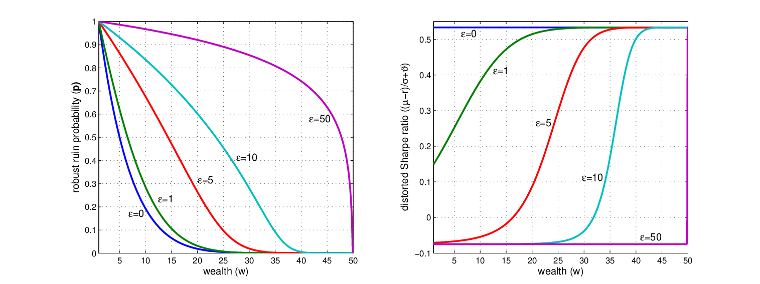
Figure 1 shows plots for the robust ruin probability $\mathfrak{p}$ and the optimally distorted Sharpe ratio $\frac{\mu-r}{\sigma}+\vartheta$ with parameters $c=1$, $b=1$, $r=0.02$, $\mu=0.1$, $\sigma=0.15$ and $\varepsilon=0,1,5,10,50$. We leave out the plot for $\varpi$ since it is a simple downward sloping linear function, and is independent of $\varepsilon$. It is worth mentioning that $\varpi\geq\pi_{0}$, i.e. the individual adopts a more aggressive investment strategy when life is perpetual.

Before we move on to the general case, let us make one more remark regarding differentiability at the safe level.

Our goal in this section is to show the nonlinear degenerate elliptic Dirichlet problem

where

has a unique viscosity solution satisfying certain properties. Notice that $F$ can be written as the supremum of a family of continuous functions, hence is lower semi-continuous (l.s.c.).

We first prove a comparison principle for (4.1) which implies uniqueness. The proof is a slight modification of the classical comparison argument to take care of the unboundedness of the control space. It turns out, luckily, that the nonlinear term $\varepsilon(u^{\prime})^{2}$ does not add any difficulty.

References

• [1] A. D. Alexandroff. Almost everywhere existence of the second differential of a convex function and some properties of convex surfaces connected with it. Leningrad State Univ. Annals [Uchenye Zapiski] Math. Ser., 6:3–35, 1939.
• [2] O. Alvarez, J.-M. Lasry, and P.-L. Lions. Convex viscosity solutions and state constraints. J. Math. Pures Appl. (9), 76(3):265–288, 1997.
• [3] Nicole Bäuerle and Erhan Bayraktar. A note on applications of stochastic ordering to control problems in insurance and finance. Stochastics, 86(2):330–340, 2014.
• [4] E. Bayraktar, X. Hu, and V. R. Young. Minimizing the probability of lifetime ruin under stochastic volatility. Insurance Math. Econom., 49(2):194–206, 2011.
• [5] E. Bayraktar and S. Yao. A weak dynamic programming principle for zero-sum stochastic differential games with unbounded controls. SIAM J. Control Optim., 51(3):2036–2080, 2013.
• [6] E. Bayraktar and V. R. Young. Correspondence between lifetime minimum wealth and utility of consumption. Finance Stoch., 11(2):213–236, 2007.
• [7] E. Bayraktar and V. R. Young. Minimizing the probability of lifetime ruin under borrowing constraints. Insurance Math. Econom., 41(1):196–221, 2007.
• [8] E. Bayraktar and V. R. Young. Minimizing the probability of ruin when consumption is ratcheted. N. Am. Actuar. J., 12(4):428–442, 2008.
• [9] E. Bayraktar and V. R. Young. Proving regularity of the minimal probability of ruin via a game of stopping and control. Finance Stoch., 15(4):785–818, 2011.
• [10] A. Ben-Tal, D. Bertsimas, and D. B. Brown. A soft robust model for optimization under ambiguity. Oper. Res., 58(4, part 2):1220–1234, 2010.
• [11] G. Bordigoni, A. Matoussi, and M. Schweizer. A stochastic control approach to a robust utility maximization problem. In Stochastic analysis and applications, volume 2 of Abel Symp., pages 125–151. Springer, Berlin, 2007.
• [12] A. Cartea, R. Donnelly, and S. Jaimungal. Robust market making. 2013. Available at SSRN: http://ssrn.com/abstract=2310645.
• [13] M. G. Crandall, H. Ishii, and P.-L. Lions. User’s guide to viscosity solutions of second order partial differential equations. Bull. Am. Math. Soc., New Ser., 27(1):1–67, 1992.
• [14] D. Duffie, W. H. Fleming, H. M. Soner, and T. Zariphopoulou. Hedging in incomplete markets with HARA utility. J. Econom. Dynam. Control, 21(4-5):753–782, 1997.
• [15] W. H. Fleming and D. Hernández-Hernández. On the value of stochastic differential games. Commun. Stoch. Anal., 5(2):341–351, 2011.
• [16] W. H. Fleming and P. E. Souganidis. On the existence of value functions of two-player, zero-sum stochastic differential games. Indiana Univ. Math. J., 38(2):293–314, 1989.
• [17] L. P. Hansen and T. J. Sargent. Robustness. Princeton University Press, 2007.
• [18] L. P. Hansen, T. J. Sargent, G. Turmuhambetova, and N. Williams. Robust control and model misspecification. J. Econom. Theory, 128(1):45–90, 2006.
• [19] D. Hernández-Hernández and A. Schied. A control approach to robust utility maximization with logarithmic utility and time-consistent penalties. Stochastic Process. Appl., 117(8):980–1000, 2007.
• [20] Y. Hu and M. Schweizer. Some new BSDE results for an infinite-horizon stochastic control problem. In Advanced mathematical methods for finance, pages 367–395. Springer, Heidelberg, 2011.
• [21] C. Huang and H. Pagès. Optimal consumption and portfolio policies with an infinite horizon: existence and convergence. Ann. Appl. Probab., 2(1):36–64, 1992.
• [22] S. Jacka. Avoiding the origin: a finite-fuel stochastic control problem. Ann. Appl. Probab., 12(4):1378–1389, 2002.
• [23] J. Jacod and A. N. Shiryaev. Limit Theorems for Stochastic Processes. Srpinger, 2nd edition, 2002.
• [24] S. Jaimungal. Irreversible investments and ambiguity aversion. 2011. Available at SSRN: http://ssrn.com/abstract=1961786.
• [25] S. Jaimungal and G. Sigloch. Incorporating risk and ambiguity aversion into a hybrid model of default. Math. Finance, 22(1):57–81, 2012.
• [26] K. Janeček and M. Sîrbu. Optimal investment with high-watermark performance fee. SIAM J. Control Optim., 50(2):790–819, 2012.
• [27] I. Karatzas and S. E. Shreve. Brownian Motion and Stochastic Calculus. Springer, 2nd edition, 1991.
• [28] N. V. Krylov. Nonlinear Elliptic and Parabolic Equations of the Second Order. D. Reidel Publishing Company, Dordrecht, Holland, 1987.
• [29] A. E. B. Lim and J. G. Shanthikumar. Relative entropy, exponential utility, and robust dynamic pricing. Oper. Res., 55(2):198–214, 2007.
• [30] P. Maenhout. Robust portfolio rules and asset pricing. The Review of Financial Studies, 17(4):951–983, 2004.
• [31] S. Mataramvura and B. Øksendal. Risk minimizing portfolios and HJBI equations for stochastic differential games. Stochastics, 80(4):317–337, 2008.
• [32] M. A. Milevsky and C. Robinson. Self-annuitization and ruin in retirement. N. Am. Actuar. J., 4(4):112–129, 2000. With discussion.
• [33] V. C. Pestien and W. D. Sudderth. Continuous-time red and black: how to control a diffusion to a goal. Math. Oper. Res., 10(4):599–611, 1985.
• [34] L. C. G. Rogers. Optimal Investment. Springer Berlin Heidelberg, 2013.
• [35] A. Schied. Optimal investments for risk- and ambiguity-averse preferences: a duality approach. Finance Stoch., 11(1):107–129, 2007.
• [36] S. E. Shreve and H. M. Soner. Optimal investment and consumption with transaction costs. Ann. Appl. Probab., 4(3):609–692, 1994.
• [37] Mihai Sîrbu. Stochastic Perron’s method and elementary strategies for zero-sum differential games. SIAM J. Control Optim., 52(3):1693–1711, 2014.
• [38] D. W. Stroock. Lectures on Stochastic Analysis: Diffusion Theory. Cambridge University Press, 1987.
• [39] A. E. Taylor. L’Hospital’s rule. Amer. Math. Monthly, 59:20–24, 1952.
• [40] N. Touzi. Optimal Stochastic Control, Stochastic Target Problems, and Backward SDE. Springer New York Heidelberg Dordrecht London, 2012.
• [41] R. Uppal and T. Wang. Model misspecification and underdiversification. The Journal of Finance, 58(6):2465–2486, 2003.
• [42] V. R. Young. Optimal investment strategy to minimize the probability of lifetime ruin. N. Am. Actuar. J., 8(4):105–126, 2004.
• [43] T. Zariphopoulou. Consumption-investment models with constraints. SIAM J. Control Optim., 32(1):59–85, 1994.