Cascading Failures in Power Grids –
Analysis and Algorithms
Abstract
This paper focuses on cascading line failures in the transmission system of the power grid. Recent large-scale power outages demonstrated the limitations of percolation- and epid- emic-based tools in modeling cascades. Hence, we study cascades by using computational tools and a linearized power flow model. We first obtain results regarding the Moore-Penrose pseudo-inverse of the power grid admittance matrix. Based on these results, we study the impact of a single line failure on the flows on other lines. We also illustrate via simulation the impact of the distance and resistance distance on the flow increase following a failure, and discuss the difference from the epidemic models. We then study the cascade properties, considering metrics such as the distance between failures and the fraction of demand (load) satisfied after the cascade (yield). We use the pseudo-inverse of admittance matrix to develop an efficient algorithm to identify the cascading failure evolution, which can be a building block for cascade mitigation. Finally, we show that finding the set of lines whose removal has the most significant impact (under various metrics) is NP-Hard and introduce a simple heuristic for the minimum yield problem. Overall, the results demonstrate that using the resistance distance and the pseudo-inverse of admittance matrix provides important insights and can support the development of efficient algorithms.
1 Introduction
Recent failures of the power grid (such as the 2003 and 2012 blackouts in the Northeastern U.S. [1] and in India [2]) demonstrated that large-scale failures will have devastating effects on almost every aspect in modern life. The grid is vulnerable to natural disasters, such as earthquakes, hurricanes, and solar flares as well as to terrorist and Electromagnetic Pulse (EMP) attacks [45]. Moreover, large scale cascades can be initiated by sporadic events [1, 2, 44].

Therefore, there is a need to study the vulnerability of the power transmission network. Unlike graph-theoretical network flows, power flows are governed by the laws of physics and there are no strict capacity bounds on the lines [10]. Yet, there is a rating threshold associated with each line – if the flow exceeds the threshold, the line will eventually experience thermal failure. Such an outage alters the network topology, giving rise to a different flow pattern which, in turn, could cause other line outages. The repetition of this process constitutes a cascading failure [19].
Previous work (e.g., [47, 18, 17] and references therein) assumed that a line/node failure leads, with some probability, to a failure of nearby nodes/lines. Such epidemic based modeling allows using percolation-based tools to analyze the cascade’s effects. Yet, in real large scale cascades, a failure of a specific line can affect a remote line and the cascade does not necessarily develop in a contiguous manner. For example, the evolution of the the cascade in India on July 2012 appears in Fig. 1. Similar non-contiguous evolution was observed in a cascade in Southern California in 2011 [44, 11] and in simulation studies [11, 12].
Motivated by this observation, we study the properties of the cascade and introduce algorithms to identify the cascading failure evolution and vulnerable lines. We employ the (linearized) direct-current (DC) power flow model,11 1 The DC model is commonly used in large-scale contingency analysis of power grids [14, 13, 40]. which is a practical relaxation of the alternating-current (AC) model, and the cascading failure model of [25] (see also [14, 13, 12, 11]). Specifically, we first review the model and the Cascading Failure Evolution (CFE) Algorithm that has been used to identify the evolution of the cascade [19, 14, 13] (its complexity is , where is the number of nodes and is the number of cascade rounds).
Then, in order to investigate the impact of a single edge failure on other edges, we use matrix analysis tools to study the properties of the admittance matrix of the grid22 2 An admittance matrix represents the admittance of the lines in a power grid with nodes. and Moore-Penrose Pseudo-inverse [4] of the admittance matrix. In particular, we provide a rank-1 update of the pseudo-inverse of the admittance matrix after a single edge failure.
We use these results along with the resistance distance and Kirchhoff’s index notions33 3 These notions originate from Circuit Theory and are widely used in Chemistry [30]. to study the impact of a single edge failure on the flows on other edges. We obtain upper bounds on the flow changes after a single failure and study the robustness of specific graph classes. We also illustrate via simulations the relation between the flow changes after a failure and the distance (in hop count) and resistance distance from the failure in the U.S. Western interconnection as well as Erdős-Rényi [26], Watts and Strogatz [46], and Barábasi and Albert [9] graphs. These simulations show that there are cases in which an edge flow far away from the failure significantly increases. These average case observations are clearly in contrast to the epidemic-based models.
We then consider the impact of a cascade. We consider a few metrics: yield (the fraction of demand satisfied after the cascade), number of line failures, number of cascade rounds, and the distance between consecutive failures. We generalize the results of [12] and show that in the worst cases, an initial single line failure may have severe effects while any super-set of failures that includes that line have minor effects. We then show that the metric values may be arbitrarily large or small (in case of the yield) even for a single initial line failure. We also prove that cascading failures may happen within arbitrarily long distance of each other and can last a large number of rounds. These characteristics are significantly different from those of the epidemic-based models. Finally, we show that a minor parameter change may have a significant impact.
Once lines fail, there is a need for low complexity algorithms to control and mitigate the cascade. Hence, we develop the low complexity Cascading Failure Evolution – Pseudo-inverse Based (CFE-PB) Algorithm for identifying the evolution of a cascade that may be initiated by a failure of several edges. The algorithm is based on the rank-1 update of the pseudo-inverse of the admittance matrix. We show that its complexity is ( is the number of edges that eventually fail). Namely, if (one edge fails at each round), the complexity of the CFE-PB Algorithm is times lower than that of the CFE Algorithm. The main advantage of the CFE-PB Algorithm is that it leverages the special structure of the pseudo-inverse to identify properties of the underlying graph and to recompute an instance of the pseudo-inverse from a previous instance.
Finally, we prove that the problems of finding the set of failures (of at most a given size) with the largest impact under different metrics, are NP-hard (or hard to approximate). For the problem of finding the set of initial failures of size that causes a cascade resulting with the minimum possible yield (minimum yield problem), we introduce a very simple heuristic termed the Most Vulnerable Edges Selection – Resistance distance Based (MVES-RB) Algorithm. We numerically show that solutions obtained by it lead to a much lower yield than the solutions obtain by selecting the initial edge failures randomly. Moreover, in some small graphs with a single edge failure, it obtains the optimal solution.
The main contributions of this paper are two fold. First, we provide new tools, based on matrix analysis for assessing the impact of a single edge failure. Using these tools, we (i) obtain upper bounds on the flow changes after a single failure, (ii) develop a fast algorithm for identifying the evolution of the cascade, and (iii) develop a heuristic algorithm for the minimum yield problem. Second, we analyze the cascade properties analytically and via simulations.
This paper is organized as follows. Section 2 reviews related work. Section 3 describes the power flow, cascade model, metrics, and the graphs used in the simulations. In Section 4, we derive the properties of the admittance matrix of the grid. Section 5 presents the effects of a single edge failure and Section 6 provides the unique properties of the cascade. Section 7 introduces the CFE-PB Algorithm. Section 8 discusses the hardness of the problems associated with the cascade and introduces the MVES-RB Algorithm. Section 9 provides concluding remarks and directions for future work. The proofs appear in the appendices.
2 Related Work
Network vulnerability to attacks has been thoroughly studied (e.g., [36, 3, 39, 31] and references therein). However, most previous computational work did not consider power grids and cascading failures. Recent work on cascades focused on probabilistic failure propagation models (e.g., [47, 18, 17], and references therein). However, real cascades [1, 2, 44] and simulation studies [11, 12] indicate that the cascade propagation is different than that predicted by such models.
In Sections 4 and 7, we use the admittance matrix of the grid to compute flows. This is tightly connected to the problem of solving Laplacian systems. Solving these systems can be done with several techniques, including Gaussian elimination and LU factorization [27]. Recently, [20] designed algorithms that use preconditioning, to provide highly precise approximate solutions to Laplacian systems in nearly linear time. However, this approach only provides approximate solutions and is not suitable for analytical studies of the effects of edge failures.
In Section 5, we obtain upper bounds on the flow changes after a single failure and study the robustness of graph classes based on resistance distance and Kirchhoff’s index [30, 16]. Recently, these notions have gained attention outside the Chemistry community. For instance, they were used in network science for detecting communities within a network, and more generally the strength of the connection between nodes in a network [37, 35]. Moreover, [22] recently used the resistance distance to partition power systems into zones.
The problem of identifying the set of failures with the largest impact was studied in [14, 13, 40, 33]. In particular, [14] studies the problem which focuses on finding a small cardinality set of links whose removal disables the network from delivering a minimum amount of demand. A broader network interdiction problem in which all the components of the network are subject to failure was studied in [43]. A similar problem is studied in [40] using the alternating-current (AC) model. However, none of the previous works consider the cascading failures. Moreover, while the optimal power flow problem has been shown to be NP-hard [32], the complexity of the cascade-related problems was not studied yet.
Finally, for the simulations, we use graphs that can represent the topology of the power grid. The structure of the power grids has been widely studied [46, 9, 6, 5, 24, 18, 23]. In particular, Watts and Strogatz [46] suggested the small-world graph as a good representative of the power grid, based on the shortest paths between nodes and the clustering coefficient of the nodes. Barabási and Albert [9, 18] showed that scale-free graphs are better representatives based on the degree distribution. However, [23] indicated that none of these models can represent U.S. Western interconnection properly. Following these papers, we consider the Erdős-Rényi graph [26] in addition to these graphs.
3 Models and Metrics
3.1 DC Power Flow Model
We adopt the linearized (or DC) power flow model, which is widely used as an approximation for the more accurate non-linear AC power flow model [10]. In particular we follow [11, 12, 14, 13] and represent the power grid by an undirected graph where and are the set of nodes and edges corresponding to the buses and transmission lines, respectively. is the active power supply () or demand () at node (for a neutral node ). We assume pure reactive lines, implying that each edge is characterized by its reactance .
Given the power supply/demand vector and the reactance values, a power flow is a solution of:
| (1) | |||
| (2) |
where is the set of neighbors of node , is the power flow from node to node , and is the phase angle of node . Eq. (1) guarantees (classical) flow conservation and (2) captures the dependency of the flow on the reactance values and phase angles. Additionally, (2) implies that . Note that the edge capacities are not taken into account in determining the flows. When the total supply equals the total demand in each connected component of , (1)-(2) has a unique solution [14, lemma 1.1].44 4 The uniqueness is in the values of -s rather than -s (shifting all -s by equal amounts does not violate (2)). Eq.(1)-(2) are equivalent to the following matrix equation:
| (3) |
where is the vector of phase angles and is the admittance matrix of the graph , defined as follows:
If there are multiple edges between nodes and , then . Notice that when , the admittance matrix is the Laplacian matrix of the graph [15]. Once is computed, the power flows, , can be obtained from (2).
Throughout this paper denotes the Euclidean norm of the vector and the operator matrix norm. For matrix , denotes its entry, its row, and its transpose.
-
Input: A connected graph and an initial edge failures event .
3.2 Cascading Failure Model
The Cascading Failure Evolution (CFE) Algorithm described here is a slightly simplified version of the cascade model used in [25, 12, 14]. We define and assume that an edge has a predetermined power capacity , which bounds its flow (that is, ). The cascade proceeds in rounds. Denote by the set of edge failures in the round and by the set of edge failures until the end of the round (). We assume that before the initial failure event , the power flows satisfy (1)-(2), and . Upon a failure, some edges are removed from the graph, implying that it may become disconnected. Thus, within each component, the total demand is adjusted to be equal to the total supply. For any set of failures , we denote by the flow along edges in after the load shedding.


Following an initial failure event , the new flows are computed (by (1)-(2)) (Line 4). Then, the set of new edge failures is identified (Line 5). Following [25, 12, 14], we use a deterministic outage rule and assume, for simplicity, that an edge fails once the flow exceeds its capacity: .55 5 Note that [25, 12, 14] maintain moving averages of the values to determine which edges fail. Therefore, .
If the set of new edge failures is empty, then the cascade is terminated. Otherwise, the process is repeated while replacing the initial event by the failure event , and more generally replacing by at the round (Line 5). The process continues until the system stabilizes, namely until no edges are removed. Finally, we obtain the sequence of the sets of failures associated with the initial event , and the power flows at stabilization, where is the number of rounds until the network stabilizes. Since solving a system of linear equations with variables, requires time [27], the output can be obtained in time.
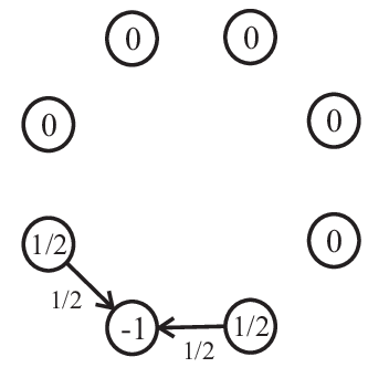
An example of a cascade can be seen in Fig. 2. Initially, the flows are for all edges. The initial set of failures () disconnects a demand node from the graph. Hence, intuitively, one may not expect a cascade. However, this initial failure not only causes further failures but also causes failures in all edges except for two. This example can be generalized to a graph with nodes where with the same set of initial failures, all the edges fail except for two.
For simplicity, when the initial failure event contains a single edge, , we denote the flows after the failure by and the flow changes by .
3.3 Metrics
We define the metrics for evaluating the grid vulnerability (some of which were defined in [12]). To study the effects of a single edge () failure after one round, we define the ratio between the change of flow on an edge, , and its original value or the flow value on the failed edge, :
Edge flow change ratio: .
Mutual edge flow change ratio: .
Below, we define metrics related to the evaluation of the cascade severity for a given instance , an initial failure event , and an integer . An instance is composed of a connected graph , supply/demand vector , capacities and reactance values , . For brevity, an instance is represented by .
Yield (the ratio between the demand supplied at stabilization and the original demand): , .
Number of edge failures: ,
.
Number of rounds until stabilization: ,
.
For the following metric, we define: (i) as the distance (in hop count) between edges and in , and (ii) for any , .
Distance between failures: , .
3.4 Graphs Used in Simulations
The simulation results are presented for the graphs described below. All graphs have 1,374 nodes to correspond the subgraph of the Western interconnection. The parameters are as indicted below, unless otherwise mentioned.
Western interconnection: 1708-edge connected subgraph of the U.S. Western interconnection. The data is from
the Platts Geographic Information System [41].
Erdős-Rényi graph [26]: A random graph where each edge appears with probability .
Watts and Strogatz graph [46]: A small-world random graph where each node connects to other nodes and the probability of rewiring is .
Barábasi and Albert graph [9]: A scale-free random graph where each new node connects to other nodes at each step following the preferential attachment mechanism.
4 Admittance Matrix Properties
In this section, we use the Moore-Penrose Pseudo-inverse of the admittance matrix [4] in order to obtain results that are used throughout the rest of the paper. Specifically they are used in Section 5 to study the impact of a single edge failure on the flows on other edges and in Section 7 to introduce an efficient algorithm to identify the evolution of the cascade. We prove several properties of the Pseudo-inverse of the admittance matrix , denoted by .66 6 [4]. For more information regarding the definition, see Appendix. always exists regardless of the structure of the graph . Some proofs and results that are used in the proofs appear in Appendix A.

Observation 1 shows that the power flow equations can be solved by using .
Observation 1
Proof 4.1.
Jointly verifying whether an edge is a cut-edge and finding the connected components of the graph takes (using Depth First Search [21]). The following two Lemmas show that by using the precomputed pseudo-inverse of the admittance matrix, these operations can be done in and , respectively. The algorithm in Section 8.2 uses the results to check if the pseudo-inverse should be recomputed. Moreover, Lemma 4.2 is crucial for the proof of the Theorem 4.5, below.
Lemma 4.2 (Bapat [8]).
Given and , all the cut-edges of the graph can be found in time. Specifically, an edge is a cut-edge if, and only if, .
Lemma 4.3.
Given , , and the cut-edge , the connected components of can be identified in .
In the following, we denote by the admittance matrix of the graph and by the power vector after removing an arbitrary edge from the graph and conducting the corresponding load shedding.
Lemma 4.4.
Given graph , , and a cut-edge , then is a solution of (3) in .
The following theorem gives an analytical rank-1 update of the pseudo-inverse of the admittance matrix. Using Theorem 4.5 and Corollary 4.6, in Section 5 we provide upper bounds on the mutual edge flow change ratios (). We note that a similar result to Theorem 4.5 was independently proved in a very recent technical report [42].
Theorem 4.5.
Given graph , the admittance matrix , and , if is not a cut-edge, then,
in which is an vector with in entry, in entry, and 0 elsewhere.
For the following, recall from Section 3 that .
Corollary 4.6.
Finally, Lemma 4.7, gives the complexity of the rank-1 update provided in Theorem 4.5. This is used in the computation of the running time of the algorithm in Section 7.
Lemma 4.7.
Given graph , , and an edge , which is not a cut-edge of the graph, can be computed from in .
We now define the notion resistance distance [30]. In resistive circuits, the resistance distance between two nodes is the equivalent resistance between them. It is known that the resistance distance, is actually a measure of distance between nodes of the graph [8]. For any network, this notion can be defined by using the pseudo-inverse of the Laplacian matrix of the network. Specifically, it can be defined in power grid networks by using the pseudo-inverse of the admittance matrix, .
Definition 4.8.
Given , , and , the resistance distance between two nodes is . Accordingly, the resistance distance between two edges is .
When all the edges have the same reactance, , the resistance distance between two nodes is a measure of their connectivity. Smaller resistance distance between nodes and indicates that they are better connected. Fig. 3 shows the relation between the distance and the resistance distance between nodes in the graphs defined in Subsection 3.4 (all the edges have the reactance equal to 1). As can be seen, there is no direct relation between these two measures in Erdős-Rényi and Barábasi-Albert graphs. However, in the Western interconnection and Watts-Strogatz graph the resistance distance increases with the distance.
In Chemistry, the sum over the resistance distances between all pairs of nodes in the graph is referred to as the Kirchhoff index [16] of and denoted by . We use this notion in Subsection 5.2.2 to study the robustness of different graph classes to single edge failures.
Definition 4.9.
Given and , the Kirchhoff index of is .
5 Effects of a Single Edge Failure
In this section we provide upper bounds on the flow changes after a single edge failure and study the robustness of different graph classes.

For simplicity, in this section, we assume that , unless otherwise indicated. As mentioned in Section 3, in this case the admittance matrix of the graph, , is equivalent to the Laplacian matrix of the graph. However, all the results can be easily generalized.
5.1 Flow Changes
5.1.1 Edge Flow Change Ratio
In order to provide insight into the effects of a single edge failure, we first present simulation results. The simulations have been done in Python using NetworkX library. Fig. 4 shows the edge flow change ratios () as the function of distance () from the failure for over 40 different random choices of an initial edge failure, . The power supply/demand in the Western interconnection is based on the actual data. In other graphs, the power supply/demand at nodes are i.i.d. Normal random variables with a slack node to equalize the supply and demand. Notice that if the initial flow in an edge is close to zero, the edge flow change ratio on that edge can be very large. Thus, to focus on the impact of an edge failure on the edges with reasonable initial flows, we do not illustrate the edge flow change ratios for the edges with flow below 1% of the average flow. Yet, we observe that such edges that experience a flow increase after a single edge failure, are within any arbitrary distance from the initial edge failure.
Fig. 4 shows that after a single edge failure, there might be a very large increase in flows (edge flow change ratios up to 80, 14, 50, and 24 in Fig. 4-(a), (b), (c), and (d), respectively) and sometimes far from the initial edge failure (edge flow change ratio around 10 for edges 11- and 4-hops away from the initial failure in Fig. 4-(a) and (c), respectively). Moreover, as we observed in all of the four graphs, there are edges with positive flow increase from zero, far from the initial edge failure. These observations motivate us to prove similar results analytically (see Observation 2 in this section and Observation 5 and 6 in Section 6).
Finally, we show that by choosing the parameters in a specific way, the edge flow change ratio can be arbitrarily large.
Observation 2
For any , there exists a graph and two edges such that
.
5.1.2 Mutual Edge Flow Change Ratio
We use the notion of resistance distance to find upper bounds on the mutual edge flow change ratios (). The following Lemma provides a formula for computing the flow changes after a single edge failure based on the resistance distances. It is independent of the power supply/demand distribution.
Lemma 5.10.
Given , , and , the flow change and the mutual edge flow change ratio for an edge after a failure in a non-cut-edge are,
Proof 5.11.
It is an immediate result of Corollary 4.6.

Fig. 5 illustrates the mutual edge flow change ratios after an edge failure. Recall that describes the distribution of the flow that passed through on the other edges. These values are differently distributed for different graph classes. In the next subsection, we study in detail the relation between the mutual edge flow change ratios and the graph structure.
The following Corollary gives an upper bound on the flow changes after a failure in a non-cut-edge by using the triangle inequality for resistance distance and Lemma 5.10.
Corollary 5.12.
Given , , and , the flow changes in any edge after a failure in a non-cut-edge can be bounded by,
With the very same idea, the following corollary gives an upper bound on the flow changes in a specific edge after a failure in the non-cut-edge .
Corollary 5.13.
Given , , and , the flow changes in an edge after a failure in a non-cut-edge and the mutual edge flow change ratio can be bounded by,
Corollary 5.13 directly connects the resistance distance between two edges () to their mutual edge flow change ratio (). It shows that the resistance distance, in contrast to the distance, can be used for assessing the influence of an edge failure on other edges.
We present simulations to show the relations between the mutual flow change ratios and the two distance measures. Figs. 6 and 7 show the mutual edge flow change ratio () as the function of distance () and resistance distance () from the failure, respectively. The figures show that increasing number of edges (increasing in Erdős-Rényi graph and increasing in Watts and Strogatz, and Barábasi and Albert graphs) affects the - relation more than the - relation. This suggests that the resistance distance better captures the information hidden in the structure of a graph. Both figures show a monotone relation between the mutual edge flow change ratios and the distances/resistance distances. However, this monotonicity is smoother in the case of the distance.
Moreover, Fig. 6, unlike Fig. 4, shows that after a single edge failure, the mutual edge flow change ratios decrease as the distance from the initial failure increases. Thus, it suggests that probabilistic tools may be used to model the mutual edge flow change ratios () better than the edge flow change ratios ().


5.2 Graph Robustness
We now use the upper bounds provided in Corollaries 5.12 and 5.13 to study the robustness of some well-known graph classes to single edge failures. We use the average mutual edge flow change ratio, , as the measure of the robustness. The small value of indicates that the flow changes in edges after a single edge failure is small compared to the original flow on the failed edge. In other words, the network is able to distribute additional load after a single edge failure uniformly between other edges.
We show that (i) graphs with more edges are more robust to single edge failures and (ii) the Kirchhoff index can be used as a measure for the robustness of different graph classes.
5.2.1 Robustness Based on Number of Edges
Using Corollary 5.12, it can be seen that a failure in an edge with small resistance distance between its two end nodes leads to a small upper bound on the mutual edge flow change ratios, , on the other edges. Thus, the average for is relatively a good measure of the average mutual edge flow change ratio. The following Observation shows that graphs with more edges have smaller average for , and therefore, smaller average mutual edge flow change ratio.
Observation 3
Given , the average for is .
Observation 3 implies that for a fixed number of nodes, the average resistance distance gets smaller as the number of edges increases. Therefore, graphs with more edges are more robust against a single edge failure.
5.2.2 Robustness Based on the Graph Class
Another way of computing the average mutual edge flow change ratio is to use Corollary 5.13 which implies that graphs with low average resistance distance over all pairs of nodes have the small average mutual edge flow change ratios. On the other hand, recall from Definition 4.9 that the average resistance distance over all pair of nodes is equal to Kirchhoff index of the graph divided by the number of edges. Hence, table 1 summarizes the Kirchhoff indices and corresponding average mutual edge flow change ratios for some well-known graph classes.
| Graph Class | Kirchhoff index | Average mutual edge flow change ratio () |
|---|---|---|
| Complete graph | ||
| Complete bipartite graph | ||
| Complete tripartite graph | ||
| Cycle graph | ||
| Cocktail party graph | ||
| Erdős-Rényi graph |
To complete the table, in the following lemma we compute the Kirchhoff index of the Erdős-Rényi graph as a function of .
Lemma 5.14.
For an Erdős-Rényi random graph, , is of , and therefore the average resistance distance between all pairs of nodes is of .
This Lemma shows that the average resistance distance between all pairs of nodes of an Erdős-Rényi graph is related to . Since as grows, the average number of edges in a Erdős-Rényi graph increases, this Lemma also suggests that graphs with more edges are more robust to a single edge failure. Thus, the results in this subsection are aligned with the result in Subsection 5.2.1 indicating that graphs with more edges are more robust to a single edge failure.
6 Properties of the Cascade
As shown in the previous section, due to the special structure of the power flow equations, even studying the impact of a single edge failure is not straightforward. In this section, we focus on the cascade that can be caused by a single or multiple failures. Using the metrics from Section 3.3, we show unique properties of cascade.
6.1 Non-monotone Effect of Failures
We show that a single edge failure event may have a larger effect in terms of number of rounds, number of edge failures, and yield than any failure event that is a superset of .
Observation 4
There exists a graph , an initial failure , , and , such that is a connected graph, , and .
This Observation implies that the identification of an initial failure event with the largest impact, is hard (see Section 8). In general, we cannot avoid considering a set of failures only because it is a subset of another set. We note that it is shown in [12, lemma 4.3] that an initial failure event may result in a lower yield than a failure event . However, in the special case used in [12], is disconnected. In Observation 4, we show that there exists a graph such that even when is connected, a single edge failure event causes more damage than .
6.2 Unbounded Metric Values
By using simple instances, we show that the effect of a single edge failure may be arbitrarily severe (Table 2 summarizes the results). First, we show that a single edge failure event may cause a cascading failure in which the number of cascade rounds is at the order of the number of edges, the yield is , and all edges fail.
| Metric | Worst case | ||
|---|---|---|---|
| Edge flow change ratio | Obs. 2 | ||
| Number of edge failures | Obs. 5 | ||
| Number of rounds | Obs. 5 | ||
| Yield | Obs. 5 | ||
| Distance between failures | Obs. 6 | ||
Observation 5
For any integer , there exists a graph with , such that , , and .
Then, we show that cascading failures may happen within arbitrarily long distance of each other and may last arbitrarily long time. This corresponds to the simulation results in Fig. 4 that shows a single edge failure can have a very significant impact on the flows on far edges. In [12, lemma 4.2] it was shown that cascading failures may happen within arbitrarily long distance of each other, and in [12, lemma 4.7] it was shown that they can last arbitrarily long time. Yet, we show that these two events can happen simultaneously.
Observation 6
For any , there exists a graph such that and for any , , . As a result .
6.3 Effects of Small Parameter Changes
We analyze the effect of very small changes in capacity, , or reactance, , of a single edge. We show that a failure event that has negligible effects on the original instance can have a major impact for slightly modified instances. Let and define graphs and as the replications of the graph with a small difference in a parameter value of an edge . In , ; and in , . We consider the consequences of a cascade caused by a single edge failure event (), for , , and .
Observation 7
For any and any integer , there exists a graph with , an edge , and an initial failure with , such that:
, , ; but
(i) , ,
(ii) , .
7 Efficient Cascading Failure Evolution Computation
-
Input: A connected graph and an initial edge failures event .
Based on the results we obtained in Section 4, we present the Cascading Failure Evolution – Pseudo-inverse Based (CFE-PB) Algorithm which identifies the evolution of the cascade. The CFE-PB Algorithm uses the Moore-Penrose Pseudo-inverse of the admittance matrix for solving (3). Computing the pseudo-inverse of the admittance matrix requires time. However, the algorithm obtains the pseudo-inverse of the admittance matrix in round from the one obtained in round , in time. Moreover, in some cases, the algorithm can reuse the pseudo-inverse from the previous round. Since once lines fail, there is a need for low complexity algorithms to control and mitigate the cascade, the CFE-PB Algorithm may provide insight into the design of efficient cascade control algorithms.
We now describe the CFE-PB Algorithm. It initially computes the pseudo-inverse of the admittance matrix (in time) and this is the only time in which it computes without using a previous version of . Next, starting from , at each round of the cascade, for each , it checks whether is a cut-edge (Line 4). This is done in (Lemma 4.2). If yes, based on Lemma 4.4, in Lines 5 and 6, the total demand is adjusted to equal the total supply within each connected component (in time). Else, in Line 7, after the removal of is computed in time (see Lemma 4.7). After repeating this process for each , the phase angles and the flows are computed in time (Line 8). The rest of the process is similar to the CFE Algorithm.
The following theorem provides the complexity of the algorithm (the proof is based on the Lemmas 1–4). We show that the algorithm runs in time (compared to the CFE Algorithm which runs in ). Namely, if (one edge fails at each round), the CFE-PB Algorithm outperforms the CFE Algorithms by .
Theorem 7.15.
CFE-PB Algorithm runs in time.
We notice that a similar approach (the step by step rank-1 update) can also be applied to other methods for solving linear equations (e.g., LU factorization [27]). However, as we showed in Section 5, using the pseudo-inverse allows developing tools for analyzing the effect of a single edge failure. Moreover, it supports the development of an algorithm for finding the most vulnerable edges.
8 Hardness and Heuristic
In this section, we prove that the decision problems associated with some of the metrics are NP-complete and one of the problems is not in APX. Using the results from Section 5, we introduce a heuristic algorithm for the problem of finding the set of initial failures of size that causes a cascade resulting with the minimum possible yield (minimum yield problem). We numerically show that solutions obtained by our algorithm lead to a much lower yield than the solutions obtain by selecting the initial edge failures randomly. Moreover, in some small graphs with a single edge failure, this algorithm obtains the optimal solution.
8.1 Hardness
First, we show that deciding if there exists a failure event (of size at most a given value) such that the yield after stabilization is less than a given threshold, is NP-complete.
Lemma 8.16.
Given a graph , a real number , , and an integer , the problem of deciding if is NP-complete.
We show below that deciding if there exists an initial failure event that causes a cascade with maximum number of rounds, is NP-complete. The proof is based on showing the relation between disconnecting a subset of supply nodes from the graph and choosing a subset in the Partition problem. If a disconnection exists such that the total amount of flow that reaches some central node is exactly half the total supply (equivalent to finding a solution for a corresponding instance of Partition problem), then the number of rounds is strictly greater than a given threshold. Otherwise, the number of rounds of any cascade is less than this threshold.
Lemma 8.17.
Given a graph and an integer , the problem of deciding if is NP-complete.
Finally, we prove that the problem of computing the maximum distance between consecutive edge failures is not in APX.
Lemma 8.18.
Given a graph , the problem of computing is not in APX.
8.2 Heuristic Algorithm for Min Yield

-
Input: A connected graph and an integer .

As shown in Lemma 8.16, the minimum yield problem is NP-hard. We now present a heuristic algorithm for solving this problem. We refer to it as the Most Vulnerable Edge Selection – Resistance distance Based (MVES-RB) Algorithm. From Corollary 5.12, it seems that edges with large have greater impact on the flow changes on the other edges. Based on this result, the MVES-RB Algorithm selects the edges with highest values as the initial set of failures.
The MVES-RB Algorithm is in the same category as the algorithms that identify the set of failures with the largest impact (i.e., algorithms that solve the problem [14, 33, 40]). However, none of the previous works focusing on the problem, considers cascading failures. The MVES-RB Algorithm is simpler than most of the algorithms proposed in the past. However, it is not possible to compare its performance to that of algorithms in [14, 33, 40, 43] since they use different formulations of the power flow problem.
We first compare via simulation the MVES-RB Algorithm to the optimal solution in small graphs and for a single initial edge failure. Fig. 8 shows the yield after stabilization when selecting a single edge failure based on the MVES-RB Algorithm, randomly, and optimally. All the graphs have 136 nodes. For all the edges the reactance, , and the capacity ,88 8 Following [12], we assume that the capacities are times the initial flows on the edges. is often referred to as the Factor of Safety (FoS) of the grid. Here, as in [12]. where is the initial flow on the edge. At each point, equal number of power supply and demand nodes are randomly selected and assigned values of 1 and -1. As can be seen, the MVES-RB Algorithm obtains the optimal solution in Erdős-Rényi and Barábasi-Albert graphs. However, it does not achieve the optimal solution in the Western interconnection and Watts-Strogatz graph.
Finding the optimal solution for the minimum yield problem in general case is impossible in polynomial time. Therefore, to get better insight into the performance of the MVES-RB Algorithm, we compare it with the case that edges are selected randomly. As can be seen in Fig. 8, the MVES-RB Algorithm outperforms the random selection most of the time. Fig 9 depicts this comparison for larger initial failures in the Western interconnection and the Watts-Strogatz graph. The power supplies and demands, the reactances, and the capacities are as above. It can be seen that the MVES-RB Algorithm can perform significantly better than the random selection (Fig. 9-(a) and (b)), and in some cases obtains similar performance to the random selection (Fig. 9-(c) and (d)). Notice that in these cases, both methods perform relatively good (lead to yield less than 0.02).
To conclude, despite the simplicity and low complexity of the MVES-RB Algorithm, simulations indicate that it outperforms the random selection and in simple cases obtains the optimal solution.
9 Conclusions
We studied properties of the admittance matrix of the grid and provided analytical tools for studying the impact of a single edge failure on the flows on the other edges. Based on these tools, we derived upper bounds on the flow changes after a single edge failure and discussed the robustness of different graph classes against single edge failures. We illustrated via simulations the impact of a single edge failure. Then, we proved the unique properties of the cascading failure model and introduced a pseudo-inverse based efficient algorithm to identify the evolution of the cascade. Finally, we proved that the computational problems associated with the various metrics are hard and introduced a simple heuristic algorithm to detect the most vulnerable edges.
This is one of the first steps in using computational tools for understanding the grid resilience to cascading failures. Hence, there are still many open problems. In particular, we plan to study the effect of failures on the interdependent grid and communication networks. Moreover, while due to its relative simplicity, most previous work in the area of grid vulnerability is based on the DC model, this model does not capture effects such as voltage collapse that may occur during a cascade. Hence, we plan to develop methods to analyze the cascades using the more realistic AC model.
Acknowledgement
This work was supported in part by CIAN NSF ERC under grant EEC-0812072, NSF grant CNS-1018379, and DTRA grant HDTRA1-13-1-0021.
References
- [1] U.S.-Canada Power System Outage Task Force. report on the August 14, 2003 blackout in the United States and Canada: Causes and recommendations. https://reports.energy.gov, (2004).
- [2] Report of the enquiry committee on grid disturbance in Northern region on 30th July 2012 and in Northern, Eastern and North-Eastern region on 31st July 2012, Aug. 2012. http://www.powermin.nic.in/pdf/GRID_ENQ_REP_16_8_12.pdf.
- [3] P. Agarwal, A. Efrat, S. Ganjugunte, D. Hay, S. Sankararaman, and G. Zussman. The resilience of WDM networks to probabilistic geographical failures. IEEE/ACM Trans. Netw., 21(5):1525–1538, 2013.
- [4] A. Albert. Regression and the Moore-Penrose pseudoinverse, volume 3. Academic Press, 1972.
- [5] R. Albert, I. Albert, and G. L. Nakarado. Structural vulnerability of the North American power grid. Phys. Rev. E, 69(2):025103, 2004.
- [6] L. A. N. Amaral, A. Scala, M. Barthélémy, and H. E. Stanley. Classes of small-world networks. PNAS, 97(21):11149–11152, 2000.
- [7] T. Aura, M. Bishop, and D. Sniegowski. Analyzing single-server network inhibition. In IEEE Proc. Computer Security Foundations Workshop (CSFW-13), 2000.
- [8] R. Bapat. Graphs and matrices. Springer, 2010.
- [9] A.-L. Barabási and R. Albert. Emergence of scaling in random networks. Science, 286(5439):509–512, 1999.
- [10] A. R. Bergen and V. Vittal. Power Systems Analysis. Prentice-Hall, 1999.
- [11] A. Bernstein, D. Bienstock, D. Hay, M. Uzunoglu, and G. Zussman. Sensitivity analysis of the power grid vulnerability to large-scale cascading failures. ACM SIGMETRICS Perform. Eval. Rev., 40(3):33–37, 2012.
- [12] A. Bernstein, D. Bienstock, D. Hay, M. Uzunoglu, and G. Zussman. Power grid vulnerability to geographically correlated failures - analysis and control implications. In Proc. IEEE INFOCOM’14 (to appear), Apr. 2014.
- [13] D. Bienstock. Optimal control of cascading power grid failures. Proc. IEEE CDC-ECC, Dec. 2011.
- [14] D. Bienstock and A. Verma. The problem in power grids: New models, formulations, and numerical experiments. SIAM J. Optimiz., 20(5):2352–2380, 2010.
- [15] N. Biggs. Algebraic graph theory. Cambridge university press, 1994.
- [16] D. Bonchev, A. T. Balaban, X. Liu, and D. J. Klein. Molecular cyclicity and centricity of polycyclic graphs. i. cyclicity based on resistance distances or reciprocal distances. Int. J. Quantum Chem., 50(1):1–20, 1994.
- [17] S. Buldyrev, R. Parshani, G. Paul, H. Stanley, and S. Havlin. Catastrophic cascade of failures in interdependent networks. Nature, 464(7291):1025–1028, 2010.
- [18] D. P. Chassin and C. Posse. Evaluating North American electric grid reliability using the Barabási–Albert network model. Phys. A, 355(2-4):667 – 677, 2005.
- [19] J. Chen, J. S. Thorp, and I. Dobson. Cascading dynamics and mitigation assessment in power system disturbances via a hidden failure model. Int. J. Elec. Power and Ener. Sys., 27(4):318 – 326, 2005.
- [20] P. Christiano, J. A. Kelner, A. Madry, D. A. Spielman, and S.-H. Teng. Electrical flows, Laplacian systems, and faster approximation of maximum flow in undirected graphs. In Proc. ACM STOC’11, June 2011.
- [21] T. H. Cormen, C. E. Leiserson, R. L. Rivest, and C. Stein. Introduction to algorithms. MIT press, 2009.
- [22] E. Cotilla-Sanchez, P. Hines, C. Barrows, S. Blumsack, and M. Patel. Multi-attribute partitioning of power networks based on electrical distance. IEEE Trans. Power Syst., 28(4):4979–4987, 2013.
- [23] E. Cotilla-Sanchez, P. D. Hines, C. Barrows, and S. Blumsack. Comparing the topological and electrical structure of the North American electric power infrastructure. IEEE Syst. J., 6(4):616–626, 2012.
- [24] P. Crucitti, V. Latora, and M. Marchiori. A topological analysis of the Italian electric power grid. Phys. A, 338(1):92–97, 2004.
- [25] I. Dobson, B. Carreras, V. Lynch, and D. Newman. Complex systems analysis of series of blackouts: cascading failure, critical points, and self-organization. Chaos, 17(2):026103, 2007.
- [26] P. Erdős and A. Rényi. On random graphs. Publicationes Mathematicae Debrecen, 6:290–297, 1959.
- [27] G. H. Golub and C. F. Van Loan. Matrix Computations. Johns Hopkins Studies in Mathematical Sciences, 4th edition, 2012.
- [28] I. Gutman and B. Mohar. The quasi-wiener and the Kirchhoff indices coincide. J. Chem. Inf. Comput. Sci., 36(5):982–985, 1996.
- [29] R. M. Karp. Reducibility among combinatorial problems. Springer, 1972.
- [30] D. J. Klein and M. Randić. Resistance distance. J. Math. Chem., 12(1):81–95, 1993.
- [31] J. Kleinberg, M. Sandler, and A. Slivkins. Network failure detection and graph connectivity. In Proc. ACM-SIAM SODA’04, Jan. 2004.
- [32] J. Lavaei and S. Low. Zero duality gap in optimal power flow problem. IEEE Trans. Power Syst., 27(1):92–107, 2012.
- [33] X. Liu, K. Ren, Y. Yuan, Z. Li, and Q. Wang. Optimal budget deployment strategy against power grid interdiction. In Proc. IEEE INFOCOM’13, Apr. 2013.
- [34] I. Lukovits, S. Nikolić, and N. Trinajstić. Resistance distance in regular graphs. Int. J. of Quantum Chem., 71(3):217–225, 1999.
- [35] B. H. McRae. Isolation by resistance. Evolution, 60(8):1551–1561, 2006.
- [36] S. Neumayer, G. Zussman, R. Cohen, and E. Modiano. Assessing the vulnerability of the fiber infrastructure to disasters. IEEE/ACM Trans. Netw., 19(3):1610–1623, 2011.
- [37] M. E. Newman and M. Girvan. Finding and evaluating community structure in networks. Phys. rev. E, 69(2):026113, 2004.
- [38] J. L. Palacios and J. M. Renom. Bounds for the Kirchhoff index of regular graphs via the spectra of their random walks. Int. J. Quantum Chem., 110(9):1637–1641, 2010.
- [39] C. Phillips. The network inhibition problem. In Proc. ACM STOC’93, May 1993.
- [40] A. Pinar, J. Meza, V. Donde, and B. Lesieutre. Optimization strategies for the vulnerability analysis of the electric power grid. SIAM J. Optimiz., 20(4):1786–1810, 2010.
- [41] Platts. GIS Data. http://www.platts.com/Products/gisdata.
- [42] G. Ranjan, Z.-L. Zhang, and D. Boley. Incremental computation of pseudo-inverse of Laplacian: Theory and applications. arXiv:1304.2300, Apr. 2013.
- [43] J. Salmeron, K. Wood, and R. Baldick. Analysis of electric grid security under terrorist threat. IEEE Trans. Power Syst., 19(2):905–912, 2004.
- [44] The Federal Energy Regulatory Comission (FERC) and the North American Electric Reliability Corporation (NERC). Arizona-Southern California Outages on September 8, 2011. http://www.ferc.gov/legal/staff-reports/04-27-2012-ferc-nerc-report.pdf.
- [45] U.S. Federal Energy Regulatory Commission, Dept. of Homeland Security, and Dept. of Energy. Detailed technical report on EMP and severe solar flare threats to the U.S. power grid, Oct. 2010.
- [46] D. J. Watts and S. H. Strogatz. Collective dynamics of small-world networks. Nature, 393(6684):440–442, 1998.
- [47] H. Xiao and E. M. Yeh. Cascading link failure in the power grid: A percolation-based analysis. In Proc. IEEE Int. Work. on Smart Grid Commun., June 2011.
Appendix A Preliminaries and Proofs of Results Used in Sections 4, 5 and 7
In this appendix we restate results related to the Moore-Penrose pseudo-inverse of matrix and the proofs for the results in Sections 4, 5, and 7.
In the following, matrices and denote the identity and the all- matrices, respectively.
Theorem A.1 (Moore-Penrose[4]).
For any matrix , Moore-Penrose pseudo-inverse of ,
always exists. And for any -vector , is the vector of minimum norm among those which minimize .
Theorem A.2 (Albert[4]).
For any matrices ,
where and are defined as follows
Proof A.3 (of Lemma 4.3).
Suppose that is a cut-edge of the connected graph , and . Assume that and . We show below that for any , . Moreover, for any and , . Suppose that is an arbitrary edge. Then, the solution to (1)-(2) for the power vector with and zero elsewhere is and zero elsewhere. Therefore, . On the other hand, from Observation 1, is a solution to the equivalent matrix equation (3). Since the solution with respect to power flows is unique, . From this and since (Lemma 4.2), for any and , . Thus, by using the precomputed pseudo-inverse of the admittance matrix, computing , and dividing the entries into two groups with equal values, the connected components of can be identified. This process requires time.
Proof A.4 (of Lemma 4.4).
First, from Observation 1, is a solution to (3) for the power vector in the graph . Since the solution to (1)-(2) with respect to power flows is unique, if , then is also a solution to (3) for the power vector in the graph . Therefore, we only need to prove that from . To prove this, we prove that . However, from the proof of Lemma 4.3, since is a cut-edge, the entries of have equal values at the entries in the same connected component. On the other hand, since is the power vector after load shedding, then the sum of the supplies and demands at each connected component is zero. Thus, .
Proof A.5 (of Theorem 4.5).
First we show that if is connected, then . is a real and symmetric matrix, therefore there exist an orthogonal and unitary matrix such that , in which is the diagonal matrix of eigenvalues of and is the normalized eigenvector related to eigenvalue . It is well-known that when is connected and unweighted, then the multiplicity of eigenvalue 0 of the Laplacian matrix is 1 [15]. Exactly the same result with the same approach can be obtained for weighted graph, therefore we can assume that and all other eigenvalues are nonzero. In this case . On the other hand, , therefore
in which is an matrix with in the first row and elsewhere.
Similarly we show that if has connected components with nodes, then in which
is a block matrix with matrices on the diagonal entries (with proper node indexing). Suppose has connected components. Again it is well-known that when is unweighted, multiplicity of eigenvalue 0 of the Laplacian matrix is equal to the number of connected components of graph [15]. With exactly the same reasoning it can be shown that it is also the case for weighted graph. Therefore, in this case . Suppose is the size of the connected component. With a proper indexing of nodes, it is easy to verify that , in which for , and zero elsewhere. Now similar to previous part,
Now we can prove the theorem. is a real and symmetric matrix, therefore there exist an matrix such that . Now using Theorem A.2,
Therefore, all we need to compute is matrices and . Using previous part,
Since , nodes and should be in the same connected component of . Therefore, from the structure of , and so . Using this,
Notice that is an vector, therefore is an scaler and in the second equation is . This is why it is written 1 instead of in the last equation. Since is not a cut edge, from Lemma 4.2 we have, , therefore is well-defined. Replacing and ,
which is what we wanted to prove.
Proof A.6 (of Corollary 4.6).
Proof A.7 (of Lemma 4.7).
Based on Corollary 4.6, after the removal of a non-cut edge , each entry of the pseudo inverse of the admittance matrix can be updated in time. Thus, computing from takes time.
Proof A.8 (of Observation 2).
We construct the graph as follows, , , and there are two parallel edges and between and . Set the capacities . Assume the reactances are such that .
Proof A.9 (of Corollary 5.12).
Using triangle inequality for resistance distance, we can write,
Apply these to Lemma 5.10 completes the proof.
Proof A.10 (of Corollary 5.13).
Notice that . The proof is exactly the same as the proof of Corollary 5.12.
Proof A.12 (of Lemma 5.14).
It is known that the Kirchhoff index of the graph can be written in terms of the eigenvalues of the Laplacian matrix of the graph as [28]. On the other hand,
However, when is relatively big, then each node has the degree equal to , therefore . Combining this with the equations above, we can easily see that . Thus, the average resistance distance is of .
As for the upper bound, it is shown in [38] that for a -regular graph with nodes, . Using this bound for Erdős-Rényi graph, we can write . Thus, the average resistance distance is of .
Proof A.13 (of Theorem 7.15).
Finding the pseudo inverse of the matrix requires time. Therefore, Line 1 takes time. Lines 5 and 6 in the algorithm take time and Line 7 takes , therefore the whole for loop takes at most time at each step. Using computed in the for loop, Lines 8 and 9 take time. Thus, the total running time of the algorithm is at most .
Appendix B Proofs of Results from Sections 6 and 8
In this appendix we provide the proofs for the results in Sections 6 and 8. In our proofs, for clarity we use the notations , , and instead of , , and respectively. We also use the notation to show multiple edges between nodes and .
Proof B.1 (Observation 4).
We construct the graph as follows,
Nodes. .
Active Powers. , , , and is a neutral node.
Edges. .
Capacities. for and 20 otherwise.
Reactances. All the reactances are equal to 1, except for the edge , .
It is easy to show that initial flows are feasible and can be computed as follows, for , for , for , and for .
Now set , the flows would change as follows, for , for , and for . As it can be seen and both exceed their capacities and fail. Therefore, and flows will change as follows, for , and for . As a result, flow on the edge exceeds its capacity and fails. Following this event, the supply nodes are getting disconnected from the demand node and therefore .
Now set , as the initial failure event. It is easy to show that the flows after this initial failure are feasible and have the following values, for and for . Thus, .
Proof B.2 (Observation 5).
Let be any integer. We construct the graph as follows.
Nodes. Set .
Active powers. and .
Edges. Set .
Capacities. For any , , where is such that . Set .
Reactances. For any , .
First note that for any , because all the edges have equal reactance . Thus the flow is feasible (for any , ) by the choice of .
Set . For any , . Thus, . Furthermore, for any , because by definition. Thus, .
We prove by induction that for any , , .
Suppose it is true for , , that is for any , , . We prove that it is also true for , that is . First, . Furthermore, for any , since by definition. Thus, . As a result, , , and .
Proof B.3 (Observation 6).
Without loss of generality we can assume is odd, otherwise we can proof the Observation for . Choose . We construct as follows.
Nodes. Set where , , .
Active powers. , , and .
Edges. Set where , , , and .
Capacities. for and otherwise, where is such that .
Reactances. for and 1 for , where is such that .
First, it is easy to see that initial flows are feasible and can be computed as follows, for , and for .
Claim 1.
If , then .
Proof B.4.
By strong induction on . By construction of , for any , . Thus, . But for any , because . Therefore, .
Now suppose the claim is true for , that is . By induction hypothesis, for any , , in particular . Thus, . Moreover, for any , because . Therefore, .
Claim 2.
.
Proof B.5.
By definition, . Recall that for any and , . Thus, because . In another hand by Claim 1, .
Claim 3.
If , then for any , , .
Proof B.6.
By Claim 1, . By construction of , for any , , , . As , for any , , .
Proof B.7 (Observation 7).
Let be any integer. We construct the graph as follows. (Graphs and are identical to except in the capacity and the reactance of an edge repectively. These slight modifications are detailed in the description of .)
Nodes. Set .
Active powers. .
Edges. Let . For convenience, we show the edge by .
Capacities. In , for , for , and for , where is such that .
In , for , and for .
Reactances. In , for any , . In , for any , , and , .
Now set . In , for any , . Thus, , , and .
a) Consider the graph . Note that the graph used in the proof of Observation 5 is exactly . We deduce that for any , , and so the flow is feasible. Furthermore, and .
b) Consider the graph . , so , in the other hand for any , , and so . Thus the flow is feasible in . Now, since , . Furthermore, for any , by the choice of and . Thus . Observe that the graph is exactly the graph used in the proof of Observation 5 when removing edges and . Recall that the difference between and is only the reactance of edge , that has been removed. Thus, we get , and .
Proof B.8 (Lemma 8.16).
Consider following problem:
Problem B.9.
Suppose is an instance of the classical flow problem, with a single source node and set of sink nodes . Assume demands are equal to 1 and lines have unbounded capacity (). Does a subset of edges with exist such that ? ( is set of sink nodes which get disconnected from the source node after removing set of edges .)
It is proved in [7, Theorem 7], that problem B.9 is NP-complete. We want to use this result to proof Lemma 8.16. For this reason we provide a polynomial time reduction from problem above to minimum yield problem.
Problem B.10.
Suppose is an instance of the power flow problem, with set of supply node and set of demand nodes . Assume for all , and . Assume all the lines have capacities equal to and reactances equal to 1. Is ?
Claim 4.
Proof B.11.
() Assume the answer to problem B.9 is yes. It means that there exists a set of edges with such that their removal disconnects at least of the sink nodes from the source node. Now in problem B.10, choose . Since two graphs are the same, at least of the demand nodes are disconnected from the supply node . As a result, final yield is at most . Since initial yield was , . Hence, .
() Now the other way, assume the answer to problem B.10 is yes. It means that there is an initial set of edge failures with such that . First, since all the edges have capacity equal to which is an upper bound for a flow in an edge, after initial set of failures, there is no cascade. Therefore, there is no further edge failures. Second, with the same reason, as long as a demand node is connected to the supply node, its demand can be satisfied. Now since , with initial set of failure , at least of the demand nodes are disconnected from supply node . In problem B.9 choose , since the graphs in two problems are the same, by removing set of edges from , at least of the sink nodes are disconnected from source node . Since , the answer to problem B.9 is also yes.
Proof B.12 (Lemma 8.17).
Let be an instance of the Partition problem such that . Let be any integer. We construct the graph as follows.
Nodes. Set where , , , and .
Active powers. for , and . The other nodes are neutral.
Edges. Set where , , , , , and .
Capacities.
where is such that .
Reactances. .

The graph is depicted in Fig. 10.
Using , the proof would be as follows. First, we show in Claim 5 that if , then there is no cascading failures. In other words, . Claim 6 proves that if at least one edge belongs to , then the number of rounds is at most . Claim 7 shows that is , then the number of rounds of the cascade is at most . As a corollary of Claims 5, 6, and 7, Claim 8 shows three necessary conditions to have a number of rounds at least . Finally Claims 9 and 10 prove that the number of rounds is at least if, and only if, there exists a solution for the instance of the Partition problem. In other words, the number of rounds is at least if, and only if, there exists such that the flow that go through node is exactly .
First it is easy to see that initial flows are feasible and have the following values,
Claim 5.
If , then .
Proof B.13.
Suppose . For any , if , then . Indeed, by construction of , for any , . Furthermore, for any , if , then because for any .
Claim 6.
Let be a set of initial edge failures. If , then .
Proof B.14.
For any , , let . Let for some , . By construction, for any , . Thus, for any , , , where is the number of rounds.
Suppose now that . It means that there exists , , such that and and with . A contradiction because by construction and . Thus, and .
Claim 7.
If , then .
Proof B.15.
By contradiction. Assume , and . By Claim 5, . Otherwise we would get . By Claim 6 , . Again, otherwise we would get . Thus and by initial flow values, we get:
- •
;
- •
;
- •
;
- •
For any , .
Therefore, no link exceeds its capacity and which is a contradiction with our initial assumption. Thus, if , then .
Claim 8.
Let be a set of initial edge failures. If , then , , and .
Claim 9.
If there exists a solution for the instance of the Partition problem, then there exists a set of initial edge failures such that .
Proof B.17.
Suppose there exists a solution for the instance of the Partition problem, that is there exists a subset such that . We set . By Claim 8, we set . Indeed, otherwise we would get a cascade with a number of rounds . Clearly, we have . For any , , let . We prove that for any , , . By induction on
- •
: Computation of and based on .
For any , . Furthermore, for any , we get because . Thus .
- •
Suppose it is true for , , then we prove it is also true for .
Computation of and based on .For any , , suppose . We prove that .
For any , we get . Furthermore, for any , we get because . Thus .
Finally, .
Claim 10.
If there does not exist a solution for the instance of the Partition problem, then any set of initial edge failures is such that .
Proof B.18.
Suppose there does not exist a solution for the instance of the Partition problem, that is for any subset , . For such a subset, we set .
By contradiction. Suppose there exists a set of initial edge failures such that .
By Claim 8, we set . Indeed, otherwise we would get a cascade length of size at most .
Let . There are two cases: (i) if , then . Thus, and the length of the cascade is because the supply nodes are not connected anymore to the demand node, (ii) If , then for any , . Thus, and the length of the cascade is .
Finally, there exists a set of initial edge failures such that if and only there exists a solution for the instance of the Partition problem. Thus, if and only there exists a solution for the instance of Partition problem. Furthermore, our reduction is polynomial. As the Partition problem is NP-complete [29], then the decision problem associated with is NP-complete.
Proof B.19 (Lemma 8.18).
Let be an even integer. Let be an instance of the Partition problem such that . We construct the graph as follows.
Nodes. Set where , , .
Active powers. for , and . The other nodes are neutral.
Edges. Set where and .
Capacities. for , for (where is such that . ), and otherwise.
Reactances. for , where is such that , and otherwise.

The graph is depicted in Figure 11.
Using , the proof would be as follows. First, we prove useful Claims 11, 12, 13 in order to show in Claim 14 that . Finally Claims 15 and 16 prove that the distance between edge failures is if, and only if, there exists a solution for the instance of the Partition problem. We conclude that the problem of computing the maximum possible distance between consecutive failures cannot be approximated within any constant in polynomial time, unless P=NP. In other words, the problem is not APX.
First, it is easy to see that initial flows are feasible and can be computed as follows,
Claim 11.
For any set and for any , if , then .
Proof B.20.
For any , . Thus, for any , if , then because .
Claim 12.
For any set , is either equal to or , or .
Proof B.21.
By Claim 11, . Now if fails at some point before , then it prevents to fail due to failure model. If fails before , then the flow on will be zero which means it never fails. If none of this two cases happen, then .
Claim 13.
For any set , if , then and for any , , .
Proof B.22.
By Claim 12, if , then or . However, regarding initial flows, if , then for , which means that none of these lines will ever fail. Therefore, .
Claim 14.
. In particular, if , then .
Claim 15.
If there exists a solution for the instance of the Partition problem, then .
Proof B.24.
Suppose there exists a solution for the instance of the Partition problem with integer values, that is there exists a subset such that . Let and . For any , , . Observe that for any , , , , but . Therefore, and the system become stable because supply and demand nodes get disconnected. Thus, and so . By previous claims, we get .
Claim 16.
If there does not exist a solution for the instance of the Partition problem with integer values, then for any set of initial edge failures , .
Proof B.25.
First, if , then and there is nothing left to prove. Therefore, assume . Regarding Claim 13, and for any , , . Now assume , for which and is an arbitrary subset of . Since there does not exist a solution for the instance , there are two possibilities
- 1.
. In this case for any , , . Therefore, and there is nothing left to prove.
- 2.
. In this case for any , , . Therefore, regarding the failure model fails and prevent any further edge failures. After this failure, demands and supply get disconnected. Therefore, the system stabilizes. Thus , and .
Therefore, in the both cases, and the proof is complete.
From Claims 16 and 15, we can conclude that an instance of the Partition problem with integer values have a solution if, and only if . Since can be built from in polynomial time, if we can approximate in polynomial time by any constant, then we can check in polynomial time whether or not. Which means that the Partition problem can be decided in polynomial time if, and only if can be approximated by a constant in polynomial time. Now since the partition problem is well-known to be NP-hard, is not in APX.