Geodesic Density Tracking with Applications to Data Driven Modeling

We use the terms “distribution” and “ensemble” interchangeably with the common meaning of the availability of a multitude of real measurements at a fixed time. Also, we assume that the underlying true dynamics generating the measurements is smooth enough [7] so that the realizations are absolutely continuous, and hence we can talk about “densities” in lieu of “distributions”. The optimal transport framework described in this paper will work even if this assumption is violated [6], namely if the distributions exist but the densities don’t.

Notice that the observations are in distributional or density level, does not necessarily imply that the underlying state dynamics is governed by a partial differential equation (PDE) or stochastic differential equation (SDE). Indeed, the density may arise from the parametric and initial condition uncertainties, although the underlying state dynamics may be deterministic, governed by an (unknown) ordinary differential equation (ODE). In this sense, the term “density” refers to the concentration of trajectories, and since the state space mass is preserved under the action of the flow, one can interpret [8] the trajectory concentration as probability density in the sense of propensity [9]. On the other hand, it may indeed be the case that the underlying true dynamics generating the observations, is governed by a SDE, naturally giving rise to probability densities, even if the initial conditions and parameters are fixed. Also, in cases where the observable is naturally distributed over spatial dimensions (e.g. a color image), then one can suitably normalize the data to enable our density-based optimal transport framework. Hence, without loss of generality, we term the observations as probability density functions (PDFs).

The idea of PDF control is not new in the control literature. Previous works like [10, 11, 12] dealt with asymptotic density shaping, meaning the feedback controls were found so that the desired PDF coincides with the stationary PDF of the closed-loop dynamics. Similar ideas predate in terms of covariance control [13]. The framework presented in this paper differs from the existing literature in that we track the distributions observed over finite horizons, and the time instances of distributional measurement availability need not be equi-spaced. The question then becomes: “over any given horizon, what needs to be done at the realization level trajectory dynamics, such that we track the observations at the ensemble level in some optimal sense?” The optimal transport theory allows us to achieve finite-time distributional tracking while guaranteeing that minimum amount of work is done over each horizon.

Most notations are standard. The symbol $\sharp$ denotes push-forward of a probability measure. $\ker\left(.\right)$ and $\text{Im}\left(.\right)$ refer to the kernel and image of a linear operator, respectively. The symbol “Id” denotes identity vector map of appropriate dimension. The notation $x\sim\rho$ means that the random vector $x$ has the joint PDF $\rho\left(x\right)$. Furthermore, $\nabla$ denotes the gradient operator with respect to spatial variables, and $\text{det}\left(\cdot\right)$ refers to determinant of a matrix. The symbol $\text{Hess}\left(\cdot\right)$ stands for the Hessian. Unless otherwise specified, the superscript ^⋆ refers to optimality, while the superscript ^† refers to the Moore-Penrose pseudo-inverse of a matrix. The notation $I$ denotes the identity matrix, $\mathcal{N}\left(\mu,\Sigma\right)$ denotes Gaussian PDF with mean $\mu$ and covariance $\Sigma$, $\mathcal{U}\left(\cdot\right)$ denotes uniform PDF.

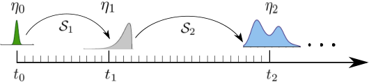
We consider a sequence of time instances $\{t_{j}\}_{j=0}^{M}$, when the measurement vector $y\left(t\right)\in\mathbb{R}^{d}$ is recorded as a sequence of PDFs $\{\eta_{j}\triangleq\eta\left(y\left(t_{j}\right),t_{j}\right)\}_{j=0}^{M}$. If we introduce $y_{j}\triangleq y\left(t_{j}\right)$, then we have $y_{j}\sim\eta_{j}$. The general problem statement can now be stated as follows (see Fig. 1).

To understand the problem, let $dm_{j\rightarrow j+1}\triangleq\rho\left(y_{j},y_{j+1}\right)\>dy_{j}dy_{j+1}$, which is nothing but the differential mass over the product space $\mathbb{R}^{2d}$. If the cost per unit mass equals squared Euclidean distance $\parallel y_{j+1}-y_{j}\parallel_{\ell_{2}\left(\mathbb{R}^{d}\right)}^{2}$, then (1) denotes the total cost to transport the density $\eta_{j}$ to $\eta_{j+1}$, while preserving mass (since both $\eta_{j}$ and $\eta_{j+1}$ are PDFs). Notice that the total cost depends on the choice of the PDF $\rho\left(y_{j},y_{j+1}\right)$ supported over $\mathbb{R}^{2d}$, that dictates the transportation policy, and hence $\mathcal{S}_{j+1}$. However, finding the joint PDF $\rho\left(y_{j},y_{j+1}\right)$ with given marginals $\eta_{j}$ and $\eta_{j+1}$, is not unique. Thus, we seek to find that transportation policy or joint PDF $\rho\left(y_{j},y_{j+1}\right)$, which is the minimizer of the total transportation cost (1).

Notice that Problem 1 is rather generic in the sense, it does not impose any structural constraint on the dynamical system $\mathcal{S}_{j+1}$ to be determined. In the context of dynamic data driven modeling, we are interested in three variants of Problem 1, stated next.

This paper is structured as follows. In Section II, the necessary background on optimal transport theory is given. In particular, we connect different formulations of optimal transport with the different dynamic data driven modeling problems described in the previous subsection, and show how they lead to different types of numerical solutions. Next, using the ideas from Section II, we discuss Problem 1.1, 1.2 and 1.3 in Sections III, IV and V, respectively. To illustrate the solution methodology, analytical and numerical results are provided for example problems. Section VI concludes the paper.

The optimal transport theory originated in 1781 when Gaspard Monge considered [14] the problem of moving a pile of soil from an excavation to another site that entails minimum work. This idea went mostly unnoticed for 160 years until Leonid Kantorovich provided a modern treatment [15] of this subject in 1942 (the English translation [16] appeared in 1958), which eventually led to the Nobel prize in economics in 1975. In the theory of Monge-Kantorovich optimal transport, one defines a distance, called Wasserstein distance, between two given PDFs $\rho$ and $\widehat{\rho}$, that measures the shape difference between them.

Instead of solving (2), one could directly solve for the the optimal transport map $\beta:\mathbb{R}^{d}\mapsto\mathbb{R}^{d}$, that satisfies $y=\beta\left(\widehat{y}\right)$, by solving

From Remark 9, we can substitute $\beta=\nabla\psi$ in the push-forward constraint $c\left(\beta\right)=0$. Then it follows that $\psi$ must solve

This is a second order, nonlinear, stationary, elliptic PDE, known as the Monge-Ampère equation, to be solved for $\psi$ as a function of $\widehat{y}$. In principle, if we can solve (6), then $\nabla\psi$ would solve Problem 1. However, as mentioned in the third row of Table I, numerically solving the PDE (6) remains a research challenge.

Benamou and Brenier proposed [23] a dynamic reformulation of the static optimization problem (4) by introducing a synthetic notion of time, which we denote as $s\in[0,\tau]$. Their main result is that the spatial optimization problem (4), is equivalent to solving the following space-time optimization problem:

One merit of the Benamou-Brenier approach described in Section II.D is that it constructs the transportation path, which is a geodesic connecting the source and target PDFs, and yields the intermediate PDFs satisfying McCann’s displacement interpolation [27]. In particular, the following results [6] hold.

1. 1.

   Without loss of generality, let the synthetic time $s\in\left[0,1\right]$, i.e. in the notation of Section II.D, set $\tau=1$. Then the Benamou-Brenier vector field constructs the geodesic curve between $\left(\widehat{\rho},\rho\right):s\in\left[0,1\right]\mapsto\varphi\left(s\right)$. Recall that the PDF $\widehat{\rho}$ is the source PDF, and $\rho$ is the target PDF. In other words, $\varphi$ has the variational characterization

   $\displaystyle\varphi\left(s\right)=\underset{\varphi}{\text{argmin}}\left(1-s\right)W^{2}\left(\widehat{\rho},\varphi\right)\>+\>sW^{2}\left(\rho,\varphi\right),$

   (10)

   and it lies on the geodesic curve connecting $\widehat{\rho}$ and $\rho$. The Wasserstein distance $W\left(\widehat{\rho},\rho\right)$ is the length of this geodesic curve on the manifold of PDFs.
   

2. 2.

   As a corollary of the above result, the intermediate optimal transport map $\beta_{s}$ that satisfies $\varphi\left(s\right)=\beta_{s}\>\sharp\>\widehat{\rho}$, is obtained via linear interpolation between the identity map Id and $\beta$, i.e.

   $\displaystyle\beta_{s}=\left(1-s\right)\text{Id}+s\beta.$

   (11)

   Also, the intermediate Wasserstein distance is obtained via linear interpolation:

   	$\displaystyle W\left(\widehat{\rho},\varphi\left(s\right)\right)$	$\displaystyle=$	$\displaystyle s\>W\left(\widehat{\rho},\rho\right),$		(12)
   	$\displaystyle W\left(\rho,\varphi\left(s\right)\right)$	$\displaystyle=$	$\displaystyle\left(1-s\right)\>W\left(\widehat{\rho},\rho\right).$		(13)

   However, the intermediate PDF is obtained via nonlinear (displacement) interpolation:

   	$\displaystyle\varphi\left(s\right)$	$\displaystyle=$	$\displaystyle\beta_{s}\>\sharp\>\widehat{\rho}=\left[\left(1-s\right)\text{Id}+s\beta\right]\>\sharp\>\widehat{\rho},$		(14)
   		$\displaystyle=$	$\displaystyle\beta_{1-s}\>\sharp\>\rho=\left[s\>\text{Id}+(1-s)\beta\right]\>\sharp\>\rho.$		(15)

Consider a linear system $x_{j+1}=Ax_{j}+Bu_{j}$, $x_{j}\in\mathbb{R}^{d},u_{j}\in\mathbb{R}^{m}$, with a sequence of Gaussian PDFs $\eta_{j}=\mathcal{N}\left(\mu_{j},\Sigma_{j}\right)$, $j=0,1,\ldots,M$. The objective is to find state feedback $u_{j}^{\star}\triangleq u^{\star}\left(x_{j}\right)$ over each time interval $\Delta t_{j}\triangleq[t_{j},t_{j+1})$, such that $x_{j}\sim\eta_{j}=\mathcal{N}\left(\mu_{j},\Sigma_{j}\right)$, while guaranteeing minimal transportation cost (1). Using the idea of Section II.B, we transcribe the problem of finding optimal control $u_{j}^{\star}$ to that of finding the optimal transport map (a.k.a. Brenier map) $\beta_{j}^{\star}:x_{j}\mapsto x_{j+1}$, where

subject to the constraints (C1) $x_{j}\sim\eta_{j}$, (C2) $\beta\left(x_{j}\right)\sim\eta_{j+1}$, and (C3) $\eta_{j+1}=\beta\>\sharp\>\eta_{j}$. Then we have the following result.

In recent years, a set of tools have been developed [31, 32, 1] for finite-horizon distribution shaping using open-loop control signal, under the constraint that the same open-loop excitation is applied to all realizations of the system dynamics (characterized by parametric dispersions). Our approach of solving Problem 1.1 is different from this paradigm, termed as “ensemble control”, in at least two ways. First, the ensemble control seeks an open-loop solution while ours is closed-loop solution. Second, the ensemble controllability needs to be established to guarantee the existence of such open loop excitation, however, if found, will allow sensor-less ensemble shaping. On contrary, our feedback implementation requires sensing at the ensemble level, but guarantees geodesic transport over each horizon.

We formulate the model refinement problem (Fig. 6) as the natural successor of the distributional model validation formulation proposed in [18, 19]. In the validation problem, the model predicted output PDF $\widehat{\eta}$ is compared with the experimentally observed output PDF $\eta$, at each instance of measurement availability $t_{j}$, $j=0,1,\ldots,M$, and an inference is made by looking at the prediction-observation gap quantified via $W\left(t_{j}\right)$. The key insight behind our refinement formulation is that usually there is no specific requirement on the structure of the refined model, as long as we can make the refined dynamics track the observed output PDFs. This provides us the freedom to formulate the model refinement problem over the model’s output map while keeping the model’s state equation intact. This has two implications: (i) the refinement algorithm will involve the output dimension $d$, typically less than the state dimension, and (ii) both state and output modeling errors would be accounted by updating the model’s output map. To make the ideas precise, we give the model refinement problem statement for a model whose output map is given by $\widehat{y}=\widehat{h}\left(\widehat{x}\right)$, where $\widehat{x}$ and $\widehat{y}$ are model-predicted state and output vectors.

At $t=t_{j}$, let us introduce $\widehat{y}_{j}^{-}\triangleq\widehat{y}_{j}$, and denote $\widehat{h}^{-}\left(\cdot\right)\triangleq\widehat{h}\left(\cdot\right)$. We want to find the Brenier map $\beta_{j}\left(\cdot\right)$ for updating the predicted output, i.e. $\widehat{y}_{j}^{+}=\beta_{j}\left(\widehat{y}_{j}^{-}\right)$, where $\widehat{y}_{j}^{+}\sim\eta_{j}$ and $\widehat{y}_{j}^{-}\sim\widehat{\eta}_{j}$. In other words, find $\beta_{j}\left(\cdot\right)$ such that $\eta_{j}=\beta_{j}\>\sharp\>\widehat{\eta}_{j}$. Clearly, this problem is underdetermined since there are many ways to morph $\widehat{\eta}_{j}$ to $\eta_{j}$. Then we must look for an optimal push-forward map $\beta_{j}^{\star}\left(\cdot\right)$ that would require minimum amount of transport effort among all possible push-forward maps $\beta_{j}\left(\cdot\right)$, i.e. we solve (4). Once $\beta_{j}^{\star}\left(\cdot\right)$ has been found, the refined model is given by augmenting the model’s state equation with the new output map:

References

- [1] J.-S. Li, and N. Khaneja, “Ensemble Control of Bloch Equations”, IEEE Transactions on Automatic Control. Vol. 54, No. 3, pp. 528–536, 2009.
- [2] H. Wang, “Robust Control of the Output Probability Density Functions for Multivariable Stochastic Systems with Guaranteed Stability”, IEEE Transactions on Automatic Control. Vol. 44, No. 11, pp. 2103–2107, 1999.
- [3] H. Wang, H. Baki, and P. Kabore, “Control of Bounded Dynamic Stochastic Distributions using Square Root Models: An Applicability Study in Papermaking Systems”. Transactions of the Institute of Measurement and Control. Vol. 23, No. 1, pp. 51–68, 2001.
- [4] E. Brown, J. Moehlis, and P. Holmes, “On the Phase Reduction and Response Dynamics of Neural Oscillator Populations”. Neural Computation. Vol. 16, No. 4, pp. 673–715, 2004.
- [5] T. White, Hadoop: The Definitive Guide, O’Reilly Media, 3rd Edition, 2012.
- [6] C. Villani, Topics in Optimal Transportation. Graduate Studies in Mathematics, First ed., American Mathematical Society; 2003.
- [7] R.J. DiPerna, and P-L. Lions, “Ordinary Differential Equations, Transport Theory and Sobolev Spaces”. Inventiones Mathematicae, Vol. 98, No. 3, pp. 511–547, 1989.
- [8] A. Lasota, and M. Mackey, Chaos, Fractals and Noise: Stochastic Aspects of Dynamics, Applied Mathematical Sciences, Vol. 97, Springer-Verlag, New York, 1994.
- [9] J.C. Willems, “Discussion on: “Why Is Resorting to Fate Wise? A Critical Look at Randomized Algorithms in Systems and Control” ”. European Journal on Control, Vol. 16, No. 5, pp. 436–440, 2010.
- [10] M. Forbes, J.F. Forbes, and M. Guay, “Regulatory Control Design for Stochastic Processes: Shaping the Probability Density Function”. Proceedings of the 2003 American Control Conference, Vol. 5, pp. 3998–4003, 2003.
- [11] C.X. Zhu, W.Q. Zhu, and Y.F. Yang, “Design of Feedback Control of A Nonlinear Stochastic System for Targeting A Pre-specified Stationary Probability Distribution”. Probabilistic Engineering Mechanics, Vol. 30, pp. 20–26, 2012.
- [12] L. Guo, and H. Wang, “Generalized Discrete-time PI Control of Output PDFs Using Square Root B-spline Expansion”. Automatica, Vol. 41, No. 1, pp. 159–162, 2005.
- [13] A.F. Hotz, and R.E. Skelton, “A Covariance Control Theory”. 24th IEEE Conference on Decision and Control, Vol. 24, pp. 552–557, 1985.
- [14] G. Monge, “Mémoire sur la thèorie des déblais et des remblais”. Histoire de l’Académie Royale des Sciences de Paris, pp. 666–704, 1781.
- [15] L.V. Kantorovich, “On the Translocation of Masses”. Comptes Rendus (Doklady) de l’Académie des Sciences de l’URSS, Vol. XXXVII, No. 7-8, pp. 199–201, 1942.
- [16] L.V. Kantorovich, “On the Translocation of Masses”. Management Science, Vol. 5, No. 1, pp. 1–4, 1958.
- [17] S.T. Rachev, Probability Metrics and the Stability of Stochastic Models. John Wiley, First ed., 1991.
- [18] A. Halder, and R. Bhattacharya, “Model Validation: A Probabilistic Formulation”, IEEE Conference on Decision and Control, Orlando, Florida, 2011.
- [19] A. Halder, and R. Bhattacharya, “Further Results on Probabilistic Model Validation in Wasserstein Metric”, IEEE Conference on Decision and Control, Maui, 2012.
- [20] Y. Brenier, “Polar Factorization and Monotone Rearrangement of Vector-valued Functions”. Communications on Pure and Applied Mathematics, Vol. 44, No. 4, pp. 375–417, 1991.
- [21] E. Haber, T. Rehman, and A. Tannnenbaum, “An Efficient Numerical Method for the Solution of the Optimal Mass Transfer Problem”. SIAM Journal on Scientific Computing, Vol. 32, No. 1, pp. 197–211, 2010.
- [22] X. Feng, R. Glowinski, and M. Neilan, “Recent Developments in Numerical Methods for Fully Nonlinear Second Order Partial Differential Equations”. SIAM Review, Vol. 55, No. 2, pp. 205–267, 2013.
- [23] J.D. Benamou, and Y. Brenier, “A Computational Fluid Mechanics Solution to the Monge-Kantorovich Mass Transfer Problem”. Numerische Mathematik, Vol. 84, No. 3, pp. 375–393, 2000.
- [24] A. Halder, and R. Bhattacharya, “Dispersion Analysis in Hypersonic Flight During Planetary Entry Using Stochastic Liouville Equation”. Journal of Guidance, Control and Dynamics, Vol. 34, No. 2, pp. 459–474, 2011.
- [25] M. Fortin, and R. Glowinski, Augmented Lagrangian Methods: Applications to the Numerical Solution of Boundary-value Problems. Vol. 15, North Holland, 1983.
- [26] N. Papadakis, G. Peyré, and E. Oudet, “Optimal Transport with Proximal Splitting”. arXiv preprint, arXiv:1304.5784, 2013.
- [27] R.J. McCann, “A Convexity Principle for Interacting Gases”. Advances in Mathematics, Vol. 128, No. 1, pp. 153–179, 1997.
- [28] I. Olkin, and F. Pukelsheim, “The Distance Between Two Random Vectors with Given Dispersion Matrices”. Linear Algebra and its Applications, Vol. 48, pp. 257–263, 1982.
- [29] M. Knott, and C.S. Smith, “On the Optimal Mapping of Distributions”. Journal of Optimization Theory and Applications, Vol. 43, No. 1, pp. 39–49, 1984.
- [30] A. Ohara, and T. Kitamori, “Geometric Structures of Stable State Feedback Systems”. IEEE Transactions on Automatic Control, Vol. 38, No. 10, pp. 1579–1583, 1993.
- [31] J.-S. Li, Control of Inhomogeneous Ensembles. Ph.D. thesis, Harvard University, 2006.
- [32] J.-S. Li and N. Khaneja, “Ensemble Control on Lie Groups”. 7th IFAC Symposium on Nonlinear Control Systems, 2007.