PUC-Logic

• •

  If Oswald did not kill Kennedy, then someone else did.

• •

  If Oswald had not killed Kennedy, then someone else would have.[1]

The phrases above are respectively instances of the indicative and the subjunctive conditionals. The indicative conditional is associated to the material implication, whereas the subjunctive construction of the language is traditionally studied by the philosophy as the counterfactual conditional[1, 3] or the counterfactual for short.

Conditional propositions involve two components, the antecedent and the consequent. Counterfactual conditionals differ from material implication in a subtle way. The truth of a material implication is based on the actual state-of-affairs. From the knowledge that Kennedy was killed, we can accept the truth of the phrase. On the other hand, a counterfactual conditional should take into account the truth of the antecedent, even if it is not the case. The truth of the antecedent is mandatory in this analysis.

Some approaches to counterfactuals entail belief revision, particularly those based on Ramsey test evaluation [11]. In this analysis, the truth value of a counterfactual is considered within a minimal change generated by admitting the antecedent true[3].

A possible way to circumvent belief revision mechanisms is to consider alternative (possible) state-of-affairs, considered here as worlds, and, based on some accessibility notion, choose the closest one among the worlds that satisfy the antecedent. If the consequent is true at this considered world, then the counterfactual is also true[1].

Both conditionals have false antecedents and false consequents in the current state-of-affairs. However, the second conditional is clearly false, since we found no reason to accept that, in the closest worlds in which Kennedy is not killed by Oswald, Kennedy is killed by someone else.

We choose the approach of Lewis[1] in our attempt to formalize an inference system for counterfactuals because his accessibility relation leaves out the discussion for a general definition of similitude among worlds, which is considered as given in his analysis.

It also opened the possibility for a contribution in the other way. If we found some general properties in his accessibility relation, considering the evaluation of the formulas in the counterfactual reasoning, we could sketch some details of the concepts of similitude.

Lewis, in the very first page of his book[1]:

”If kangaroos had no tails, they would topple over, seems to me to mean something like this: in any possible state of affairs in which kangaroos have no tails, and which resembles our actual state of affairs as much as kangaroos having no tails permits it to, the kangaroos topple over.”

We can observe that the word “resemble” may be seen as a reference to the concept of similarity between some possible state of affairs in relation to the actual state of affairs. The expression “as much as” here may be understood as a relative comparison of similarities among the possible states of affairs in relation to the actual state of affairs. But Lewis gave no formal definition of similarity in his book[1].

He used possible-world semantics for intentional logic. For that reason the state of affairs are treated as worlds. To express similarity, he used proximity notions: a world is closer to the actual world in comparison to other worlds if it is more similar to the actual world than other considered worlds.

Lewis called the set of worlds to be considered for an evaluation as the strictness of the conditional. He pointed out that the strictness of the counterfactual conditional is based on the similarity of worlds. He showed that the counterfactual could not be treated by strict conditionals, necessity operators or possibility operators given by modal logics. To do so, he argued that strictness of the conditional can not be given before all evaluations. He constructed sequences of connected counterfactuals in a single English sentence for which the strictness cannot be given for the evaluation:

”If Otto had come, it would have been a lively party; but if both Otto and Anna had come it would have been a dreary party; but if Waldo had come as well, it would have been lively; but…”

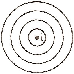
Lewis proposed a variably strict conditional, in which different degrees of strictness is given for every world before the evaluation of any counterfactual. To express this concept, the accessibility relation is defined by a system of spheres, which is given for every world by a nesting function $\$$ that applies over a set of worlds $\mathcal{W}$. The nested function attributes a set of non-empty sets of worlds for each world and this set of sets is in total order for the inclusion relation.

A systems of spheres, of any kind, is central in the most traditional analysis of counterfactuals. But the idea behind it is also available to many different logics. So, if we manage to handle them in a satisfactory manner, we will be able to use it in a broader class of logics. The system of neighbourhoods facilitates the development of the model, by leaving open the choice for a proper definition of similarity. And that concept can be used for a broader class of logics, not only the counterfactuals.

From Lewis definitions, the nesting function is a primitive notion:

$\phi\boxright\psi$ is true at a world $i$ (according to a system of spheres $\$$) if and only if either: no $\phi$-world belongs to any sphere $S$ in $\$_{i}$¹¹ 1 $\$_{i}$ gives the neighbourhoods around the world $i$. They are the available strictness to evaluate counterfactuals at $i$., or some sphere $S$ in $\$_{i}$ does contains at least one $\phi$-world, and $\phi\rightarrow\psi$ holds at every world in $S$.

$\phi\preccurlyeq\psi$ is true at a world $i$ (according to a system of spheres $\$$) if and only if, for every sphere $S$ in $\$_{i}$, if $S$ contains any $\psi$-world then $S$ contains a $\phi$-world.

Lewis[1] also provided conditions that may be applied to the nesting function $\$$. To every condition corresponds a different counterfactual logic:

• •

  Normality (N): $\$$ is normal iff $\forall w\in\mathcal{W}:\$(w)\neq\emptyset$;

• •

  Total reflexivity (T): $\$$ is totally reflexive iff $\forall w\in\mathcal{W}:w\in\bigcup\$(w)$;

• •

  Weak centering (W): $\$$ is weakly centered iff $\forall w\in\mathcal{W}:\$(w)\neq\emptyset\mbox{ and }\forall N\in\$(w):w\in N$ ;

• •

  Centering (C): $\$$ is centered iff $\forall w\in\mathcal{W}:\{w\}\in\$(w)$;

• •

  Limit Assumption (L): $\$$ satisfies the Limit Assumption iff, for any world $w$ and any formula $\phi$, if there is some $\phi$-world²² 2 A $\phi$-world is a world in which $\phi$ holds. in $\bigcup\$(w)$, then there is some smallest sphere of $\$(w)$ that contains a $\phi$-world;

• •

  Stalnaker’s Assumption (A): $\$$ satisfies Stalnaker’s Assumption iff, for any world $w$ and any formula $\phi$, if there is some $\phi$-world in $\bigcup\$(w)$, then there is some sphere of $\$(w)$ that contains exactly one $\phi$-world;

• •

  Local Uniformity (U-): $\$$ is locally uniform iff for any world $w$ and any $v\in\bigcup\$(w)$, $\bigcup\$(w)$ and $\bigcup\$(v)$ are the same;

• •

  Uniformity (U): $\$$ is uniform iff for any worlds $w$ and $v$, $\bigcup\$(w)$ and $\bigcup\$(v)$ are the same;

• •

  Local absoluteness (A-): $\$$ is locally absolute iff for any world $w$ and any $v\in\bigcup\$(w)$, $\$(w)$ and $\$(v)$ are the same;

• •

  Absoluteness (A): $\$$ is absolute iff for any worlds $w$ and $v$, $\$(w)$ and $\$(v)$ are the same.

The $\boldsymbol{V}$-logic is the most basic counterfactual logic presented by Lewis[1], where “V” stands for variably strict conditional. If, for example, we accept the centering condition (C), then we have the $\boldsymbol{VC}$-logic. Lewis showed in his book a chart of 26 non-equivalent $\boldsymbol{V}$-logics that arises from the combinations of the conditions.

We prefer to call the spheres as neighbourhoods, because they represent better the concept of proximity, which Lewis used to express similarity. The neighbourhoods provide a relative way to compare distance. The world that is contained in a neighbourhood is closer to the actual world than other world that is not contained in that same neighbourhood.

As far as we know, there is only one natural deduction system for the counterfactuals, which is given by Bonevac [13]. But his system is designed to deals with the $\boldsymbol{VW}$-logic, since it contains the rule of counterfactual exploitation ($\boxright$E), which encapsulates the weak centering condition. His approach to define rules for the counterfactual operators provides a better intuition of the counterfactual logic. His systems is expressive enough to deal with modalities and strict conditionals. The labelling of world shifts using formulas make easier to capture the counterfactual mechanics.

We also found the work of Sano [14] which pointed out the advantages of using the hybrid formalism for the counterfactual logic. He presented some axioms and rules for the $\boldsymbol{V_{\mathcal{HC}(@)}}$-logic that extends the $\boldsymbol{V}$-logic of Lewis.

Another interesting reference is the article of Gent[12], which presents a new sequent- or tableaux-style proof system for V C. His work depends on the operator $\llbracket\rrbracket$ and the definition of signed formulas.

We recently found a sequent calculus, provided by Lellmann[25], that treats the $\boldsymbol{V}$-logic of Lewis and its extensions. Its language depends on modal operators, specially the counterfactual operators $\boxright$ and $\boxRight$ and the comparative possibility operator $\preccurlyeq$.

As far as we know, our deduction system is the only one dealing with Lewis systems in a general form, that is, without using modalities in the syntax and treating the most basic counterfactual $\boldsymbol{V}$-logic.

In [17], we presented a sequent calculus for counterfactual logic based on a Local Set Theory [4]. In this article, we defined the satisfaction relation for worlds, for sets of the worlds and for neighbourhoods, where we encapsulated some quantifications that made it easier to express the operators with fewer quantifiers. But the encapsulation made the the inference system to have no control of the quantifications. Here we propose a logic for Proximity-based Understanding of Conditionals, PUC-Logic for short, that take control of the quantifications with labels.

We use the term structure to refer a model or a template.

We now define a relation between structures to represent the pertinence of neighbourhoods in a neighbourhood system of a world and the pertinence of worlds in a given neighbourhood.

One remark: if the size of a path is even, then a model is related to another model or a template is related to another template.

We introduce labels in our language, in order to syntactically represent quantifications over two specific domains: neighbourhoods and worlds. So, for that reason, a label may be a neighbourhood label or a world label:

• •

  Neighbourhood labels:

  • ($\circledast$)

    Universal quantifier over neighbourhoods of some neighbourhood system;

  • ($\circledcirc$)

    Existential quantifier over neighbourhoods of some neighbourhood system;

  • ($N$)

    Variables (capital letters) that may denote some neighbourhood of some neighbourhood system.

• •

  World labels:

  • ($\ast$)

    Universal quantifier over worlds of some neighbourhood;

  • ($\bullet$)

    Existential quantifier over worlds of some neighbourhood;

  • ($u$)

    Variables (lower case letters) that denote some world of some neighbourhood.

We denote the set of neighbourhood labels by $\boldsymbol{L}_{n}$ and the set of world labels by $\boldsymbol{L}_{w}$.

As in the case of labels, we want to separate the sets of well-formed formulas into two disjoint sets, according to sort of label that labels the formula. We denote the set of neighbourhood formulas by $\boldsymbol{F}_{n}$ and the set of world formulas by $\boldsymbol{F}_{w}$.

We introduced the two formulas for true and false, in order to make the sets of formulas disjoint. The formula $\shneg N$ is introduced to represent that a neighbourhood contains the neighbourhood $N$ and the formula $\shpos N$ represent a neighbourhood is contained in $N$.

The last two rules of definition 3.9 introduces the labelling the formulas. Moreover, since we can label a labelled formula, every formula has a stack of labels that represent nested labels. We call it the attribute of the formula. The top label of the stack is the index of the formula. We represent the attribute of a formula as a letter that appear to the right of the formula. If the attribute is empty, we may omit it and the formula has no index. The attribute of some formula will always be empty if the last rule, used to build the formula, is not one of the labelling rules, as in the case of $((\alpha\rightarrow\alpha)^{\circledast,\bullet})\vee(\gamma^{\circledcirc,\ast})$.

To read a labelled formula, it is necessary to read its index first and then the rest of the formula. For example, $(\alpha\rightarrow\alpha)^{\circledast,\bullet}$ should be read as: there is some world, in all neighbourhoods of the considered neighbourhood system, in which it is the case that $\alpha\rightarrow\alpha$.

We may concatenate stacks of labels and labels, using commas, to produce a stack of labels that is obtained by respecting the order of the labels in the stacks and the order of the concatenation, like $\alpha^{\Sigma,\Delta}$, where $\alpha$ is a formula and $\Sigma$ and $\Delta$ are stacks of labels. But we admit no nesting of attributes, which means that $(\alpha^{\Sigma})^{\Delta}$ is the same as $\alpha^{\Sigma,\Delta}$.

The relation defined below is motivated by the fact that, if a model $\mathcal{M}$ satisfies a formula like $\alpha^{\circledast,\ast}$, then for every template $\mathcal{T}$, such that $\mathcal{M}\multimap\mathcal{T}$, $\mathcal{T}$ satisfies $\alpha^{\circledast}$ by definition. And also for every model $\mathcal{H}$, such that $\mathcal{M}\multimap_{2}\mathcal{H}$, $\mathcal{H}$ satisfies $\alpha$ by definition.

Every rule of PUC-ND has a stack of labels, called its context. The scope is represented by a capital Greek letter at the right of each rule. The scope of a rule is the top label of its context. Given a context $\Delta$, we denote its scope by $\oc\Delta$. If the context is empty, then there is no scope. As in the case of labels and formulas, we want to separate the contexts into two disjoint sets: $\Delta\in\boldsymbol{C}_{n}$ if $\oc\Delta\in\boldsymbol{L}_{n}$; $\Delta\in\boldsymbol{C}_{w}$ if $\Delta$ is empty or $\oc\Delta\in\boldsymbol{L}_{w}$.

The wff $\alpha^{\bullet}\rightarrow\beta^{\bullet}$ and $\gamma^{u,\circledast,\ast}$ fit into the context $\{\circledcirc\}$, because $(\alpha^{\bullet}\rightarrow\beta^{\bullet})^{\circledcirc}\in\boldsymbol{F}_{n}$ and $\gamma^{u,\circledast,\ast,\circledcirc}\in\boldsymbol{F}_{n}$. The wff $\alpha^{\bullet}\vee\beta^{\ast}$ and $\gamma^{\ast,N,u}$ do not fit into the context $\{\circledcirc,\ast\}$, because $(\alpha^{\bullet}\vee\beta^{\ast})^{\ast,\circledcirc}$ and $\gamma^{\ast,N,u,\ast,\circledcirc}$ are not wff and, therefore, cannot be in $\boldsymbol{F}_{n}$. There is no wff that fits into the context $\{\ast\}$, because the label $\ast\in\boldsymbol{L}_{w}$ and the rule of labelling can only include the resulting formula into $\boldsymbol{F}_{w}$. We can conclude that if a wff is in $\boldsymbol{F}_{n}$, then the context must be in $\boldsymbol{C}_{w}$ and the same for $\boldsymbol{F}_{w}$ and $\boldsymbol{C}_{n}$. The fitting restriction ensures that the conclusion of a rule is always a wff.

Moreover, the definition of fitting resembles the attribute grammar approach for context free languages [5]. This is the main reason to name the stack of labels of a formula as the attribute of the formula.

We present here, as an example of the PUC-ND inference calculus, a proof of a tautology. Considering Lewis definitions, we understand that if there is some neighbourhood that has some $\beta^{\Omega}$-world but no $\alpha^{\Sigma}$-world, then, for all neighbourhoods, having some $\alpha^{\Sigma}$-world implies having some $\beta^{\Omega}$-world. The reason is the total order for the inclusion relation among neighbourhoods.

 ⁴[$(\neg(\alpha^{\Sigma}))^{\ast}\wedge\beta^{\Omega,\bullet})^{\circledcirc}$]      $(\neg(\alpha^{\Sigma}))^{\ast}\wedge\beta^{\Omega,\bullet})^{\circledcirc}$     $\circledcirc$   $(\neg(\alpha^{\Sigma}))^{\ast}\wedge\beta^{\Omega,\bullet}$       ³[$(\neg(\alpha^{\Sigma}))^{\ast}\wedge\beta^{\Omega,\bullet}$]    $N$       $\Pi$         $(\alpha^{\Sigma,\bullet}\rightarrow\beta^{\Omega,\bullet})^{\circledast}$   3            $(\alpha^{\Sigma,\bullet}\rightarrow\beta^{\Omega,\bullet})^{\circledast}$     4       $((\neg(\alpha^{\Sigma}))^{\ast}\wedge\beta^{\Omega,\bullet})^{\circledcirc}\rightarrow(\alpha^{\Sigma,\bullet}\rightarrow\beta^{\Omega,\bullet})^{\circledast}$

References

• (1) Lewis, D. K., “Counterfactuals”, Blackwell Publishing, 2008.
• (2) Lewis, D. K., “Papers in ethics and social philosophy”, Cambridge University Press, 2000.
• (3) Goodman, N., “Fact, Fiction, and Forecast”, 4th Edition, Harvard University Press, 1983.
• (4) Bell, J. L., “Toposes and Local Set Theories”, Dover Publications, 2008.
• (5) Knuth, D. E., “Semantics of context-free languages”, Mathematical Systems Theory 2 (1968).
• (6) Goldblatt, R., “Topoi: The categorical analysis of logic”, Dover, 2006.
• (7) Goldblatt, R., “Logics of time and computation”, CSLI lecture notes, 1992.
• (8) Prawitz, D., “Natural Deduction: a proof-theoretical study”, Dover, 2006.
• (9) do Amaral, F. N. and E. H. Haeusler, “Using the internal logic of a topos to model search spaces for problems”, Logic Journal of IGPL (2007).
• (10) Menezes, P. B. and E. H. Haeusler, “Teoria das Categorias para Ciência da Computação”, Editora Sagra Luzatto, 2006.
• (11) Ramsey, F. P., “Philosophical papers”, Cambridge University Press, 1990.
• (12) Gent, I. P., “A Sequent- or Tableau-style System for Lewis’s Counterfactual Logic VC”, Notre Dame Journal of Formal Logic, vol. 33, no. 3, pp. 369-382, 1992.
• (13) Bonevac, D., “Deduction: Introductory Symbolic Logic”, Blackwell, 2003.
• (14) Sano, K., “Hybrid counterfactual logics”, Journal of Logic, Language and Information, volume 18, No. 4, pp 515-539, 2009.
• (15) López-Escobar, E.G.K., “Implicational Logics in Natural Deduction Systems”, Journal of Symbolic Logic, Vol. 47, No. 1, pp. 184-186, 1982
• (16) Fernandes, R.Q.A., Haeusler, E.H., Pereira, L.C.P.D., “A Natural Deduction System for Counterfactual Logic”, in XVI Encontro Brasileiro de Lógica, Petrópolis, 2011.
• (17) Fernandes, R.Q.A., Haeusler, E.H., “A Topos-Theoretic Approach to Counterfactual Logic”, in Fourth Workshop on Logical and Semantic Frameworks, Brasília, 2009. Pre-proceedings, 2009.
• (18) Hansson, B., “An Analysis of some Deontic Logics”, Noûs, Vol. 3, No. 4, pp. 373-398, 1969.
• (19) van Dalen, D., “Logic and Structure”, Springer, 2008.
• (20) Libkin, L., “Elements of Finite Model Theory”, Springer, 2010.
• (21) Troelstra, A. S., Schwichtenberg, H., “Basic Proof Theory”, Cambridge University Press, 2000.
• (22) Lambert, K., “Free Logic: selected essays”, Cambridge University Press, 2004.
• (23) Cook, S. A., “The complexity of theorem proving procedures”, In 3rd Annual ACM Symposium on the Theory of Computation, pages 151-158, 1971.
• (24) Statman, R., “Intuitioinistic propositional logic is polinomial-space complete”, Journal of Theoretical Computer Science, vol. 9, no. 1, pp. 67-72, 1979.
• (25) Lellmann, B., Pattinson, D., “Sequent Systems for Lewis’ Conditional Logics”, In 13th European Conference on Logics in Artificial Intelligence, 2012.