Self-induced polar order of active Brownian particles in a harmonic trap

Understanding the non-equilibrium behavior of self-propelled particles is one of the major challenges at the interface of physics, biology, and also chemical engineering [1, 2]. Interacting active particles may show exotic phenomena such as swirling motion [3], or exhibit dynamic clustering [4, 5] and motility-induced phase separation [6, 7, 8, 9, 10]. Their collective motion drives macroscopic fluid flow as in bioconvection [11] or vortex formation [12]. Hydrodynamic interactions between microswimmers crucially determine their collective patterns [13, 14, 15, 16, 17, 18, 19, 20], while external fluid flow leads to aggregation [21], trapping [22], and nonlinear swimming dynamics [23].

In order to understand the collective dynamics of active particles and their steady-state distributions, they are often mapped onto passive systems that move in effective potentials [24, 25, 26]. However, for interacting particles there is no general route for identifying an equilibrium counterpart [6, 1, 10].

The system we investigate here is composed of self-propelled or active Brownian particles whose swimming directions undergo rotational diffusion in a harmonic trap. Bacteria or both active and passive colloids confined in optical traps have attracted experimental [27, 28, 29] as well as theoretical [30, 31, 24, 32, 33] interest. Passive colloids are operated in non-equilibrium by switching the trapping force [31] while active particles are intrinsically out of equilibrium [24, 32, 33]. Run-and-tumble particles in lattice Boltzmann simulations develop a pump state which breaks the rotational symmetry of the harmonic trap and cause a macroscopic fluid flow [32]. Here, we demonstrate similar behavior for active Brownian particles which interact by hydrodynamic flow fields. However, more importantly we explain the emerging orientational order of particles by mapping the self-induced alignment of swimmers in a harmonic potential onto an equilibrium system which exhibits ferromagnetic order.

To this end we first establish a quantitative criterion for the formation of the pump and then introduce a mean-field description for the fully formed pump state. The mean-field system shows a striking analogy to the Weiss molecular field in ferromagnetism and reproduces our Brownian dynamic simulations.

The system also bears some similarity to the vortex formation in Daphnia populations [12] caused by irradiation with light where the apparent attraction towards the center of the light spot has also been modeled by a harmonic potential [34]. The crucial difference, however, is that Daphnia swim towards the light by phototaxis whereas in the system discussed here the harmonic potential exerts a body force on the swimmers. One focus of this work is thus on the self-induced polar order of active particles and how it is mapped on a passive system with very different underlying physics.

We consider a dilute suspension of $N$ self-propelled particles with constant propulsion speed $v_{0}$ whose leading hydrodynamic interactions are modeled by (far-field) mobility tensors $\boldsymbol{\mu}_{ij}$. Particles are spherical with an internal orientation vector $\mathbf{p}_{i}$, as realized, for example, in active colloids [5, 9] and they swim with velocity $v_{0}\mathbf{p}_{i}$. The Langevin equations of motion for the position $\mathbf{r}_{i}$ and orientation $\mathbf{p}_{i}$ of particle $i$ then are

with

The particle velocity $\mathbf{v}_{i}$ thus consists of the self-propulsion term $v_{0}\mathbf{p}_{i}$ along the particle’s orientation vector, the contribution from the harmonic trapping forces acting on all particles, $\mathbf{F}_{j}=-k_{\mathrm{trap}}\mathbf{r}_{j}$, a stresslet velocity term $\mathbf{u}_{\mathrm{SS}}$ caused by the active swimming of all other particles with $\mathbf{r}_{ij}=\mathbf{r}_{i}-\mathbf{r}_{j}$, and the thermal noise term $\sum_{j=1}^{2N}\mathbf{H}_{ij}\boldsymbol{\xi}_{j}$. Here, $\boldsymbol{\xi}_{j}$ is a $3$-component vector and contains time-uncorrelated Gaussian variables with zero mean and unit variance for translational or rotational noise. The noise components are coupled to each other by the $3\times 3$ amplitude matrices $\mathbf{H}_{ij}$, which are determined by the fluctuation-dissipation theorem. Further details are found in the supplemental material. The swimmers interact hydrodynamically via the second and fourth term in $\mathbf{v}_{i}$. We consider hydrodynamic interactions up to second order in $1/r$, with $r$ the swimmer distance, and use for the translational mobility $\boldsymbol{\mu}_{ij}^{tt}$ the Oseen tensor. The velocity stresslet $\mathbf{u}_{\mathrm{SS},j}(\mathbf{r})=\beta v_{0}\frac{3a^{2}}{4r^{2}}[-3(\mathbf{p}_{j}\cdot\hat{\mathbf{r}})^{2}+1]\,\hat{\mathbf{r}}$, with $\hat{\mathbf{r}}=\mathbf{r}/r$ and particle radius $a$, determines whether a particle is an extensile (pusher, $\beta<0$), contractile (puller, $\beta>0$) or neutral ($\beta=0$) swimmer. Unless stated otherwise, we set $\beta=0$ and use the neutral swimmer as default.

Angular velocity likewise consists of a deterministic part due to the vorticity caused by the trapping force, the vorticity due to the swimmers’ flow dipoles $\boldsymbol{\omega}_{\mathrm{SS}}=1/2(\nabla\times\mathbf{u}_{\mathrm{SS}})$, and thermal rotational noise $\mathbf{H}_{(i+N)j}\boldsymbol{\xi}_{j}$. The mobility tensor $\boldsymbol{\mu}_{ij}^{rt}$ couples translational to rotational motion and in leading order of $1/r^{2}$ is given in the supplemental material. We simulate the collective dynamics of active particles using Brownian dynamics simulations with hydrodynamic interactions following an extended form of the algorithm by Ermak and McCammon [35], where the self-propulsion and swimming terms are included.

In steady state, non-interacting active particles accumulate at or near the surface of a sphere where active swimming and trapping force cancel each other. The particles’s horizon has the characteristic radius $r_{\mathrm{hor}}=a\mathrm{Pe}/\alpha$ [24], where $a$ is the particle radius, $\mathrm{Pe}=v_{0}a/D$ the active Péclet number, and $\alpha=k_{\mathrm{trap}}a^{2}/(k_{B}T)$ the trapping Péclet number with translational diffusion coefficient $D=k_{B}T/(6\pi\eta a)$. The spherical symmetry, however, is broken when hydrodynamic interactions are included. At sufficiently large $\mathrm{Pe}$, particles assemble into a pump in a more tightly packed region, where they align their swimming directions and produce a macroscopic fluid flow [32]. The situation is sketched in Fig. 1 (left) and accompanying videos can be found in the supplemental material.

Figure 1 (right) gives the state diagram for pump formation. A simple criterion for pump formation against thermal noise (lower solid line in the diagram) can be derived from a comparison of time scales. In simulations, particles first accumulate mainly at the characteristic radius $r_{\mathrm{hor}}$ of the non-interacting system without generating any macroscopic fluid flow. So translational advection but also translational noise are not important at this point, however, their orientations can freely diffuse. Therefore, the relevant criterion for particles to assemble into a pump is the following. When hydrodynamic interactions between particles are strong enough to overcome rotational diffusion, they rotate particles’ swimming directions towards spontaneously formed denser particle regions. Thus if the time scale of rotational diffusion, $T_{\mathrm{diff}}=2\pi^{2}/D_{R}$ ¹¹ 1 For thermal diffusion of spherical particles, the rotational ($D_{R}$) and translational ($D$) diffusion coefficients are connected by $D_{R}=3D/(4a^{2})$, is larger than the rotation time due to the flow field’s vorticity $T_{\mathrm{HI}}=2\pi/\omega_{\mathrm{HI}}$, particles will be rotated towards dense spots and then, by swimming towards them, further enhance those density hot spots. Estimating the net vorticity disturbance on a particle in the otherwise spherically symmetric initial state to be $\omega_{\mathrm{HI}}=k_{\mathrm{trap}}r_{\mathrm{hor}}/(8\pi\eta r_{\mathrm{nn}}^{2})$ with the nearest-neighbor distance $r_{\mathrm{nn}}\approx 4r_{\mathrm{hor}}/\sqrt{N}$, we find the pump formation criterion $\alpha\geq 4\sqrt{\mathrm{Pe}/(\pi N)}$. Details of the calculations are given in the supplemental material.

This rough estimate reproduces the onset of pump formation quite well [see lower solid line in Fig. 1 (right)]. To indicate the alignment of particle orientations in the steady state, we use the polar order parameter $\mathcal{P}_{\infty}=\lim_{t\rightarrow\infty}\left|\sum_{i=1}^{N}\mathbf{p}_{i}(t)\right|/N$ [17]. For very dense systems, particles become close-packed and no pump is formed as the upper solid curve at constant density $n=0.5$ in Fig. 1 (right) shows. At such high densities, however, the assumption of far-field interactions also no longer holds. In the following we concentrate on dilute systems and, unless stated otherwise, follow the path of the dashed line with mean density $n=10^{-3}$. To realize a constant density for different $\mathrm{Pe}$, we fix the particle number $N=100$ and keep the effective trap volume constant by varying the trapping Péclet number $\alpha$ alongside the active Péclet number $\mathrm{Pe}$ to ensure $r_{\mathrm{hor}}\propto\alpha/\mathrm{Pe}=\mathit{const.}$.

In order to gain analytical insight, we reduce the Smoluchowski equation for the $N$-particle distribution function to a mean-field equation for the one-particle distribution $\psi(\mathbf{r},\mathbf{p})$. The collective dynamics due to hydrodynamic interactions is taken into account by a mean flow field $\mathbf{u}(\mathbf{r})$ generated by all the particles. It is independent of time, once the pump has formed. The Smoluchowski equation governing the effective one-particle dynamics is

We use the translational flux $\mathbf{J}_{T}=[v_{0}\mathbf{p}+\mu_{t}\mathbf{F}_{\mathrm{ext}}(\mathbf{r})+\mathbf{u}(\mathbf{r})]\psi(\mathbf{r},\mathbf{p})$ and the rotational flux $\mathbf{J}_{R}=[(\nabla\times\mathbf{u}(\mathbf{r}))/2-D_{R}\mathcal{R}]\psi(\mathbf{r},\mathbf{p})$. Translational diffusion is neglected in $\mathbf{J}_{T}$ because of Péclet numbers $\mathrm{Pe}\gtrsim 100$, whereas rotational diffusion still needs to be included. As we assume the flow field $\mathbf{u}$ to be independent of time, Eq. (1) only describes the dynamics close to a fully formed pump state and we will just attempt to determine the steady state distribution $\psi(\mathbf{r},\mathbf{p})$.

Strictly speaking, the collective flow field follows self-consistently from the distribution $\psi(\mathbf{r},\mathbf{p})$ by integrating over all particle contributions, $\mathbf{u}(\mathbf{r})=\int\boldsymbol{\mu}(\mathbf{r}-\mathbf{r}^{\prime})\mathbf{F}_{\mathrm{ext}}(\mathbf{r^{\prime}})\psi(\mathbf{r^{\prime}},\mathbf{p^{\prime}})d\mathbf{r}^{\prime}d\mathbf{p^{\prime}}$. Here, however, we first determine the flow field from the full $N$-particle simulations, argue that it is well represented by a regularized stokeslet, and only check a posteriori that our resulting mean-field density gives rise to the same flow field.

To quantify the flow field $\mathbf{u}(\mathbf{r})$, Fig. 2 shows the directional average for the absolute value of its Fourier transform $\tilde{\mathbf{u}}(\mathbf{k})$. The average goes over all directions of wave vector $\mathbf{k}$ keeping wave number $k$ fixed. Before taking the Fourier transform, the flow field has been averaged over 100 uncorrelated simulation snapshots in the steady state to suppress fluctuations. We find that in the parameter range, where the pump is fully formed, the strength of the flow field $\mathbf{u}$ is simply proportional to the particle swimming speed $v_{0}$. As Fig. 2 demonstrates, for active Péclet number $\mathrm{Pe}=100$ the pump has not yet fully formed but for $\mathrm{Pe}=200$ to 500 all data fall on a single master curve when rescaled by $v_{0}$. They agree very well with the flow field of a regularized stokeslet [37],

also for the regions inside the pump (see Fig. 2, solid line). Here, the flow field deviates from an unregularized stokeslet (dashed line) and only in the far field (small $k$) does the flow field become a conventional stokeslet. The regularization parameter $\epsilon$ is used as a fit parameter but it turns out that it coincides with the radius of the region populated by active particles and thus can be interpreted as the pump radius. For large wave numbers $k$, the simulated flow field starts to differ from $\mathbf{u}_{\mathrm{reg}}$ as fluctuations on the scale of several particle radii become visible.

We now make an ansatz for the particle distribution $\psi(\mathbf{r},\mathbf{p})$ and assume that particle orientations always point radially outward, $\psi(\mathbf{r},\mathbf{p})=\Phi(\mathbf{p})\,f(r)\,\delta(\cos(\theta)-\cos(\theta_{p}))\delta(\varphi-\varphi_{p})$. Here $\theta$ and $\varphi$ are the spherical coordinate angles of position and $\theta_{p}$ and $\varphi_{p}$ those of orientation. The polar angles $\theta$ and $\theta_{p}$ are both measured against the main axis of the pump [see also the sketch in Fig. 1 (left)]. The assumption of parallel orientation and position vector is motivated by the system without hydrodynamic interactions at high Péclet numbers. Here, particles quickly swim to the horizon where the trapping force cancels their self-propulsion. With interactions included, the assumption of parallel orientation and position vector still holds approximately (see supplemental material). Integrating Eq. (1) over particle position using the ansatz for $\psi(\mathbf{r},\mathbf{p})$, we arrive at the equation for the orientational distribution function,

where the mean vorticity of the collective flow field is determined for the regularized stokeslet of Eq. (2): $\langle\boldsymbol{\omega}\rangle(\mathbf{p})=-D_{R}A\,\,\sin(\theta_{p})\,\mathbf{e}_{\varphi_{p}}$ with $A=\mathrm{Pe}\int_{0}^{\infty}\frac{\epsilon\,a(5\epsilon^{2}+2r^{2})}{3(\epsilon^{2}+r^{2})^{5/2}}r^{3}f(r)\mathrm{d}r$. Eq. (3) can then be solved in steady state and the orientational distribution function becomes $\Phi(\mathbf{p})=\mathrm{e}^{A\cos(\theta_{p})}/\mathcal{N}$, where $\mathcal{N}$ is a normalization factor. Figure 3 (top) shows $\Phi(\mathbf{p})$ for different active Péclet numbers in very good agreement with Brownian dynamics simulations. The radial distribution $f(r)$ necessary to determine the constant $A$ for the analytic result has been extracted from simulations.

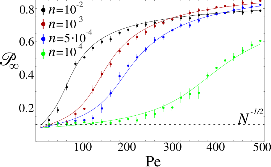
All particles thus create a mean flow field in which single swimmers align, in analogy to Weiss theory for ferromagnetism using a molecular field. Here the regularized stokeslet or more precisely the field strength $A$ takes the role of the molecular magnetic field and mean polar order $\cal{P}_{\infty}$ that of magnetization. This analogy can be made more explicit by looking at the overall alignment $\mathcal{P}_{\infty}=\int_{0}^{2\pi}\int_{-1}^{1}\mathbf{p}\,\Phi(\mathbf{p})\mathrm{d}\varphi_{p}\mathrm{d}\cos(\theta_{p})$, which evaluates to $\mathcal{P}_{\infty}=\mathcal{L}(A)=\coth(A)-1/A$ with the Langevin function $\mathcal{L}(A)$ as encountered in the classical theory of magnetism [38]. Importantly, the field strength $A$ depends in turn on the alignment $\mathcal{P}_{\infty}$ and we find in our simulations $A\propto(\mathrm{Pe}\,\mathcal{P}_{\infty})^{\gamma}$ with an exponent $\gamma$ close to 1 for low densities and decreasing for higher densities (see supplemental material). So, we indeed have a formal analogy to the Weiss molecular field generalized to an exponent $\gamma\leq 1$. The active Péclet number $\mathrm{Pe}$ takes the role of inverse temperature and a critical $\mathrm{Pe}$ can be determined.

Fig. 3 (bottom) shows alignment curves for various values of density $n$. Due to the finite number of particles $N$, the curves are shifted from 0 to $\mathcal{P}_{\infty}=N^{-1/2}$ for no alignment. Similarly, total alignment $\mathcal{P}_{\infty}=1$ cannot be attained because the shape of the pump and the excluded volume of the particles prohibit completely parallel particle orientations. The latter is taken into account via a geometric parameter $\mathcal{P}_{\infty}^{\mathrm{max}}$. The implicit equation for $\mathcal{P}_{\infty}$ becomes $(\mathcal{P}_{\infty}-N^{-1/2})/\mathcal{P}_{\infty}^{\mathrm{max}}=\mathcal{L}(3\,(\mathrm{Pe}\,\mathcal{P}_{\infty}/\mathrm{Pe}_{\mathrm{c}})^{\gamma})$, which fits the data very well when numerically solved for $\mathcal{P}_{\infty}$ with the critical Péclet number $\mathrm{Pe}_{\mathrm{c}}$ and the geometric parameter $\mathcal{P}_{\infty}^{\mathrm{max}}$ as fitting parameters. The exponent $\gamma=1.0$ for $=10^{-4}$ but decreases for higher densities and is only $\gamma=0.5$ for $n=10^{-2}$, which is likely due to excluded volume effects. The critical Péclet numbers for the different densities are found to agree roughly with the values derived from the time scale argument in Fig. 1.

We also investigated the effect of the velocity dipoles ($\beta\neq 0$) due to the particles’ swimming and found those flow stresslets to hinder alignment (Fig. 4). This is in agreement with previous studies on suspensions of active particles [17, 19]. Neutral swimmers ($\beta=0$) show the strongest ordering meaning that the alignment of swimmers is mediated solely by the stokeslets due to the trapping force, as assumed in our calculations. Our studies also show an asymmetry between pushers and pullers with alignment decreasing faster for pushers ($\beta<0$) than pullers $\beta>0$. Again this agrees with previous studies [17, 19] which explained this asymmetry by the observation that head-to-head orientations (which would contribute to $\mathcal{P}_{\infty}=0$) are stabilized for pushers due to a stagnation point in front of the swimmer in the swimming frame.

We investigated the pump formation of active Brownian particles in a harmonic trap with hydrodynamic interactions included. This is an example of a non-equilibrium system whose properties are in striking analogy to a well-known equilibrium system. Specifically, we showed that the self-induced alignment of particles mediated by the flow field they create is in formal agreement with spontaneous magnetization in ferromagnetic materials treated on the mean-field level. Here, particle orientations follow a Boltzmann distribution in an aligning mean flow field which is created by the active particles. A critical Péclet number, where pump formation sets in, can be determined in analogy to the (inverse) critical temperature of ferromagnets. The mean flow field corresponds to a single regularized stokeslet. Its strength scales linearly with the particle swimming speed and the regularization parameter $\epsilon$ gives the pump radius.

Understanding the non-equilibrium of active particles is one of the challenging questions in statistical physics right now. This Letter presents an intriguing example of a non-equilibrium system of active particles which can be mapped onto a classical equilibrium system. With recent advances in colloid physics it would be very interesting to experimentally realize the fluid pump formed by self-induced polar order and validate our predictions.