What is the physical origin of strong Ly emission?
II. Gas Kinematics and Distribution of Ly Emitters Note: accepted for publication in ApJ
Abstract
We present a statistical study of velocities of Ly, interstellar (IS) absorption, and nebular lines and gas covering fraction for Ly emitters (LAEs) at . We make a sample of 22 LAEs with a large Ly equivalent width (EW) of Å based on our deep Keck/LRIS observations, in conjunction with spectroscopic data from the Subaru/FMOS program and the literature. We estimate the average velocity offset of Ly from a systemic redshift determined with nebular lines to be km s-1. Using a Kolmogorv-Smirnov test, we confirm the previous claim of Hashimoto et al. (2013) that the average of LAEs is smaller than that of LBGs. Our LRIS data successfully identify blue-shifted multiple IS absorption lines in the UV continua of four LAEs on an individual basis. The average velocity offset of IS absorption lines from a systemic redshift is km s-1, indicating LAE’s gas outflow with a velocity comparable to typical LBGs. Thus, the ratio, of LAEs, is around unity, suggestive of low impacts on Ly transmission by resonant scattering of neutral hydrogen in the IS medium. We find an anti-correlation between Ly EW and the covering fraction, , estimated from the depth of absorption lines, where is an indicator of average neutral hydrogen column density, . The results of our study support the idea that is a key quantity determining Ly emissivity.
Subject headings
cosmology: observations — early universe — galaxies: formation — galaxies: high-redshiftI. INTRODUCTION
Ly Emitters (LAEs) are an important population of high- star-forming galaxies in the context of galaxy formation. LAEs at and beyond are found by narrow-band (NB) imaging observations based on an NB excess resulting from their prominent Ly emission [8, 24, 7, 53, 52, 54, 28, 17, 32, 31, 63, e.g., ]. Observational studies on a morphology and spectral energy distribution (SED) of LAEs reveal that such a galaxy is typically young, compact, less-massive, less-dusty than other high- galaxy populations, and a possible progenitor of Milky Way mass galaxies [23, 26, 51, 20, 11, 56, 9, e.g., ]. Additionally, LAEs are used to measure the neutral hydrogen fraction at the reionizing epoch, because Ly photons are absorbed by intergalactic medium (IGM).
Ly emitting mechanism is not fully understood due to the highly-complex radiative transfer of Ly in the interstellar medium (ISM). Many theoretical models have predicted that the neutral gas and/or dust distributions surrounding central ionizing sources are closely linked to the Ly emissivity [48, 16, 37, 39, 38, 12, 72, 71, 70, e.g., ]. Thus, resonant scattering in the neutral ISM can significantly attenuate the Ly emission.
Ly emissivity may not only depend on the spatial ISM distribution, but on the gas kinematics as well. The large-scale galactic outflows driven by starbursts or active galactic nuclei could allow Ly photons to emerge at wavelengths where the Gunn-Peterson opacity is reduced, and consequently enhance the Ly emissivity, particularly in the high- Universe [10, e.g., ]. The outflow may also blow out the Ly absorbing ISM. The gas kinematics of LAEs has been evaluated from the Ly velocity offset () with respect to the systemic redshift () traced by nebular emission lines (e.g, H, O iii) from their H ii regions. In the past few years, deep NIR spectroscopic studies have detected nebular emission lines from LAEs at , and measured their [42, 27, 25, 18, 5]. The Ly emission lines for these LAEs are redshifted from their by a of km s-1. Hashimoto et al. [27] find an anti-correlation between Ly equivalent width (EW) and in a compilation of LAE and LBG samples. This result is in contrast to a simple picture where Ly photons more easily escape in the presence of a galactic outflow.
However, the Ly velocity offset is thought to increase with both resonant scattering in H i gas clouds as well as galactic outflow velocity [69, 68, e.g., ]. The anti-correlation could result from a difference in H i column density () rather than outflowing velocity. The gas kinematics can be investigated more directly from the velocity offset between interstellar (IS) absorption lines of the rest-frame UV continuum and (IS velocity offset; ). The IS velocity offset traces the speed of outflowing gas clouds, and may help to distinguish the two effects on .
For UV-continuum selected galaxies, the has been measured for objects [55, 6, 36, 60, 66, e.g.]. Steidel et al. [66] find that LBGs have an average of km s-1 in their sample of 89 LBGs at . This statistical study indicates ubiquitousness of galactic outflow in LBGs. However, there have been no NB-selected galaxies with a measurement to date except for a stacked UV spectrum in Hashimoto et al. [27]. This is because it is difficult to estimate for individual LAEs, especially for galaxies with a large Ly EW of Å due to their faint UV-continuum emission, while are measured for some UV-selected galaxies with EW(Ly Å [13, e.g., ]. A statistical investigation of Ly kinematics for LAEs could shed light on the physical origin of the anti-correlation and the underlying Ly emitting mechanism.
This is the second paper in the series exploring the Ly emitting mechanisms11 1 The first paper presents a study on LAE structures [64].. In this paper, we present the results of our optical and NIR spectroscopy for a large sample of LAEs with Keck/LRIS and Subaru/FMOS to verify possible differences of and between LAEs and LBGs. These spectroscopic observations are in an extension of the project of Hashimoto et al. [27] aiming to confirm the anti-correlation between Ly EW and . The organization of this paper is as follows. In Section II, we describe the details of the LAEs targeted for our spectroscopy. Next, we show our optical and NIR spectroscopic observations in Section III. We present methods to reduce the spectra, and to measure kinematic quantities such as and in IV. We perform SED fitting to derive physical properties in Section V. We compare kinematic properties between LAEs and LBGs in Section VI, and discuss physical origins of possible differences in these quantities in Section VII. In the last section Section VIII, we summarize our findings.
II. TARGETS for SPECTROSCOPY
Our targets for optical and NIR spectroscopy are LAEs selected by observations of the Subaru/Suprime-Cam [43] equipped with the narrow-band (NB) filter, NB387 ( Å and FWHM Å) [47, 46]. The details of observations and selection for LAEs are given in these papers, but we provide a brief description as follows. The Suprime-Cam observations have been carried out for LAEs at with NB387 in a total area of square degrees. Based on the color selection of and , the Suprime-Cam observations have located , , , , and LAEs in the Cosmic Evolution Survey (COSMOS) [61], the Subaru/XMM-Newton Deep Survey (SXDS) [19], the Chandra Deep Field South (CDFS) [21], the Hubble Deep Field North (HDFN) [22], and the SSA22 [65, e.g., ] fields, respectively. In the above five fields, a total of LAEs have been selected down to a Ly EW of Å in rest-frame (Nakajima et al. in prep.). This large sample size enables us to study statistically various properties of high- LAEs, such as structural properties [64] and the statistics of Ly halos [44].
III. OBSERVATION
III.1. Optical Spectroscopy for Ly and UV Continuum Emission
We have carried out optical spectroscopy for our LAE sample with the Low Resolution Imaging Spectrometer [50, 67, LRIS; ] on the Keck I telescope in order to detect their redshifted Ly emission lines. We used six multi-object slit (MOS) masks for LAEs selected in the NB387 imaging observations in the COSMOS, HDFN, HUDF, SSA22, and SXDS fields. The mask for the objects in the HUDF includes two LAEs whose nebular emission lines were detected in the 3D-HST survey (H. Atek et al. in preparation). The total number of LAEs observed with these LRIS masks is 83. The observations were conducted on March 19-21 and November 14-15, 2012 (UST) with seeing sizes of -. Spectrophotometric standard stars were observed on each night for flux calibrations. The spectral resolution is . The number of observed LAEs, grisms, central wavelength and observing time in each slit-masks are summarized in Table 1.
| Slit Mask | Grating/ | Date of Observations | ||||
|---|---|---|---|---|---|---|
| [Å] | [s] | [s] | ||||
| (1) | (2) | (3) | (4) | (5) | (6) | (7) |
| COSMOS | 2012 March 19-21 | |||||
| HDFN1 | 2012 March 20 | |||||
| HDFN2 | 2012 March 19-20 | |||||
| COSMOS3B | 2012 November 15 | |||||
| HUDF_maB | 2012 November 14 | |||||
| SXDS495B | 2012 November 14-15 |
Note. — Columns: (1) Slit mask. (2) Number of objects included in the slit mask. (3). Grating and the central wavelength. (4) Exposure time of one frame. (5) Number of exposure. (6) Exposure time. (7) Date of observations.
III.2. Near-Infrared Spectroscopy for Nebular Emission
To calculate systemic redshifts of our LAEs from their nebular emission lines, we use NIR spectroscopic data obtained from observations with the Fiber Multi Object Spectrograph [34, FMOS; ] on the Subaru telescope on December 22, 23, and 24, 2012 (UST). All of LAEs in the SXDS and COSMOS fields are observed with J and H-band filters of FMOS. Details of the FMOS observation and reduction are shown in Nakajima et al. in prep. The systemic redshifts for objects were derived by simultaneously fitting to H and O iii emission lines by using their vacuum wavelengths in rest-frame.
IV. Spectroscopic Data
IV.1. Reduction of LRIS Spectra
Our LRIS spectra in each MOS mask are reduced with the public Low-Redux (XIDL) pipeline22 2 http://www.ucolick.org/ xavier/LowRedux/, for longslit and multi-slit data from the spectrographs on the Keck, Gemini, MMT, and Lick telescopes. We reduce the spectra of LAEs with this software in the following manner. First, we create flats, calibrate wavelengths with the arc data, and reject sources illuminated by the cosmic ray injections for 2-D spectra in the MOS masks. Next, we automatically identify emission lines and continua, and trace them in each slit in individual one-frame masks. After the source identification, we subtract the sky background, and correct for the distortion of the 2-D MOS mask images using sky lines. According to the information on the source identifications, we extract 1-D spectra from each slit in individual mask images. Finally, we stack the extracted 1-D spectra.
The public XIDL software extracts 1-D spectra from each one-exposure frame before combining these 2-D mask images. This process makes it difficult to detect faint emission lines and continua that are undetectable in individual one-exposure images. Then, we additionally search for faint emission lines from stacked 2-D images by visual inspection after combining one-exposure frames.
In total, the Ly emission lines are detected from 26 objects in the LRIS spectroscopy. Figure 1 shows the spectroscopic success rate in the detection of Ly emission. The success rate is % for bright objects with NB387. However, low detection and/or selection completeness at NB387 reduces largely the success rate (%). The photometric and spectroscopic properties of these Ly-detected objects are listed in Table 2. Among these LRIS spectra, we identify eight LAEs with detections of Ly and nebular emission lines excluding AGN-like objects.

IV.2. Measurement of Ly Velocity Offset
We measure the Ly velocity offset for the eight LAEs with detections of Ly and nebular lines:
| (1) |
where , , and , are the speed of light, and Ly and systemic redshifts, respectively. The systemic redshift is determined from nebular emission lines obtained with FMOS.
Prior to the measurement of , we measure the wavelength of Ly in the following line-fitting procedures. We use the peak wavelength of the best-fit asymmetric Gaussian profile for measurements of the Ly wavelength. We first search automatically for an emission line in a wavelength range of Å in each spectrum. This range includes the wavelength range of the NB387 filter. Next, we fit an asymmetric Gaussian profile to the detected lines. The asymmetric Gaussian profile is expressed as
| (2) |
where , , and are the amplitude, peak wavelength of the emission line, and continuum level, respectively. The asymmetric dispersion, , is represented by , where and are the asymmetric parameter and typical width of the line, respectively. An object with a positive (negative) value has a skewed line profile with a red (blue) wing. The fitting with the asymmetric Gaussian profile is efficient for Ly line from high- galaxies affected by complex kinematic structure of infalling and/or outflowing gas and IGM absorption. For fitting, we use data points over the wavelength range where the flux drops to % of its peak value at the redder and bluer sides of the emission line. We use the peak flux, wavelength of the line peak, , , and as the initial parameters of , , , , and for the line-fitting. The last two are typical values of our spectra. If profile fitting does not converge to the minimum in , we search for the best-fit by changing the initial value of .
We show the best-fit asymmetric Gaussian profile for an example spectrum in Figure 2. We also fit a symmetric Gaussian profile to the emission lines in addition to asymmetric one. For the symmetric Gaussian fitting, we adopt two wavelength ranges where the flux drops to % and % of its peak value, and denote the corresponding peak wavelengths by and , respectively. The fitting procedure in the former narrow range is similar as in Hashimoto et al. [27] in terms of avoiding systematic effects due to asymmetric line profile. As shown in Fig. 2, the best-fit is broadly equal to for the example line. The wavelength difference is Å( km s-1 at ). In contrast, differs from by Å which corresponds to a velocity difference of km s-1 at . This is likely to be caused by the sharp drop on the blue side and the extended red tail which cannot be fit well with symmetric profiles.

This trend is more clearly shown in Figure 3 which exhibits the wavelength difference of and from as a function of the asymmetric parameter, . The wavelengths of individual profiles are in good agreement for almost symmetric lines with . Even for moderately-asymmetric profile with , tends to correct for systematic effects of skewed lines compared to . However, both of and are redshifted (blueshifted) from by Å for highly-asymmetric lines with ().

After correcting for the heliocentric motion of Earth for the redshifts of Ly and nebular lines33 3 http://fuse.pha.jhu.edu/support/tools/vlsr.html, we calculate following Equation 1. Table 2 lists the , , and for the 26 Ly-detected objects observed with LRIS. Figure 4 present Ly spectra as a function of velocity for LAEs with detections of nebular emission lines. In Table 3, we also list these quantities of the four LAEs with detections of Ly and nebular lines obtained by previous Magellan/IMACS observations [47]. Almost all objects observed with LRIS have a of km s-1 which is consistent with values in previous studies [27, e.g., ]. The values of in the IMACS sample are calculated to be smaller than the LRIS results. This could be caused by large uncertainties due to the IMACS spectroscopy with a lower spectral resolution than LRIS.

| Slit Mask | Object | R.A. | Decl. | U | NB387 | B | EW(Ly) | |||||||
|---|---|---|---|---|---|---|---|---|---|---|---|---|---|---|
| [Å] | [erg/s/cm2] | [erg/s] | [Å] | [km s-1] | ||||||||||
| (1) | (2) | (3) | (4) | (5) | (6) | (7) | (8) | (9) | (10) | (11) | (12) | (13) | (14) | (15) |
| COSMOS | 12027 | 149.9343976 | +2.1285326 | 24.2 | 23.4 | 24.5 | 2.1906 | |||||||
| 12805bbUV continuum-detected LAEs. | 150.0637013 | +2.1354116 | 23.7 | 23.3 | 23.8 | 2.16144 | 2.15872 | |||||||
| 13138 | 150.0108585 | +2.1401388 | 24.9 | 24.6 | 25.0 | 2.18074 | 2.17921 | |||||||
| 13636bdbdfootnotemark: | 149.9974498 | +2.1439906 | 23.9 | 23.0 | 24.1 | 2.1626 | 2.16052 | ffHashimoto et al. [27] have reported that LAE 13636 has a of km s-1. However, the H line profile would have been affected by a residual of a neighboring OH line due to the low spectral resolution of their Keck-II/NIRSPEC observation (), making it difficult to determine accurately the systemic redshift. Our FMOS spectroscopy with would securely detect nebular emission less affected by OH lines. | ||||||
| 14212bbUV continuum-detected LAEs. | 149.9585714 | +2.1482830 | 24.0 | 23.3 | 24.0 | 2.19165 | 2.18955 | |||||||
| 08357aaThese objects are reduced without the Keck/LRIS public pipeline. | 149.9961405 | +2.0921070 | 24.8 | 24.4 | 24.9 | 2.18243 | 2.18044 | |||||||
| 13820aaThese objects are reduced without the Keck/LRIS public pipeline. | 149.9554179 | +2.1470628 | 25.6 | 25.1 | 25.9 | 2.14246 | ||||||||
| 14135aaThese objects are reduced without the Keck/LRIS public pipeline. | 149.9770609 | +2.1508410 | 27.0 | 25.9 | 26.8 | 2.2024 | ||||||||
| HDFN1 | 18325ccAGN-like objects. | 189.0973399 | +62.1014179 | 22.9 | 21.6 | 23.2 | 2.1742 | |||||||
| 20042aaThese objects are reduced without the Keck/LRIS public pipeline. | 189.0293966 | +62.1176510 | 25.4 | 24.7 | 25.6 | 2.17921 | ||||||||
| HDFN2 | 31902 | 189.3127706 | +62.2091548 | 25.4 | 23.9 | 24.9 | 2.17957 | |||||||
| 43408 | 189.4532215 | +62.2639356 | 26.7 | 25.4 | 26.3 | 2.19708 | ||||||||
| 42659aaThese objects are reduced without the Keck/LRIS public pipeline. | 189.4575590 | +62.2917868 | 25.9 | 23.8 | 25.9 | 2.19336 | ||||||||
| COSMOS3B | 38380 | 149.9205873 | +2.3844960 | 24.4 | 23.4 | 24.5 | 2.21616 | 2.21256 | ||||||
| 43982cdcdfootnotemark: | 149.9766453 | +2.4416582 | 24.3 | 23.2 | 24.6 | 2.19413 | 2.19333 | 0.41 | ||||||
| 46597 | 149.9415665 | +2.4688913 | 24.7 | 23.8 | 24.7 | 2.17355 | ||||||||
| 38019aaThese objects are reduced without the Keck/LRIS public pipeline. | 149.9020418 | +2.3815371 | 25.9 | 25.0 | 25.7 | 2.2084 | ||||||||
| 40792aaThese objects are reduced without the Keck/LRIS public pipeline. | 149.9444266 | +2.4094991 | 26.7 | 25.5 | 27.4 | 2.20928 | ||||||||
| 41547aaThese objects are reduced without the Keck/LRIS public pipeline. | 149.9246216 | +2.4166699 | 26.0 | 24.9 | 26.6 | 2.15224 | ||||||||
| 44993aaThese objects are reduced without the Keck/LRIS public pipeline. | 149.9744788 | +2.4530529 | 26.5 | 25.0 | 26.5 | 2.2144 | ||||||||
| HUDF_maB | 17001eeK. Nakajima et al. in preparation. | 2.04806 | ||||||||||||
| 31000eeK. Nakajima et al. in preparation. | 3.08798 | |||||||||||||
| SXDS495B | 06713 | 34.4224906 | -5.1136338 | 24.5 | 23.5 | 24.6 | 2.20332 | |||||||
| 10600bbUV continuum-detected LAEs. | 34.4420541 | -5.0486039 | 23.7 | 23.0 | 23.6 | 2.21109 | 2.20915 | |||||||
| 10942 | 34.4980945 | -5.0428800 | 25.6 | 24.2 | 25.6 | 2.19783 | 2.19557 | |||||||
| 10535aaThese objects are reduced without the Keck/LRIS public pipeline. | 34.4246768 | -5.0488535 | 25.9 | 24.8 | 26.2 | 2.21263 |
Note. — Columns: (1) Slit mask. (2) Object ID. (3) Right ascension. (4) Declination. (5)-(7) , NB387, and -band magnitudes. (8) Observed wavelength of Ly measured by the asymmetric gaussian fitting. (9) Redshift of Ly corrected for the heliocentric motion. (10) Ly flux uncorrected for slit loss in LRIS spectroscopy. (11) Ly luminosity. (12) Ly equivalent width estimated from the NB387 magnitudes. A Ly position in the transmission curve are taken into account from the spectroscopic redshift of Ly. (13) Redshift of nebular emission lines corrected for the heliocentric motion (K. Nakajima et al. in preparation.). (14) Ly velocity offset relative to nebular emission lines. (15) Ratio of Ly flux in the bluer side relative to the systemic redshift to total Ly flux.
Additionally, we provide a consistency check for our measurement of by using the same object as in Hashimoto et al. [27], COSMOS-13636. The object has been observed with both of LRIS in this work and Magellan/MagE in a previous work. The redshift of Ly estimated from the LRIS spectrum () is in good agreement with that of MagE () within a fitting error. The difference in velocity is km s-1. The large error in is likely to be due to the lower spectral resolution of LRIS () than that of MagE ().

Figure 5 shows the HST/ACS -band images of LAEs with a measurement in the COSMOS field. Unfortunately, the LAEs in the SXDS field are not covered by the CANDELS project. Several LAEs have multiple components, which could be mergers. The merger fraction of LAEs and its Ly dependence are discussed in Shibuya et al. [64].
| Object | EW(Ly) | ||||
|---|---|---|---|---|---|
| [Å] | [Å] | [km s-1] | |||
| (1) | (2) | (3) | (4) | (5) | (6) |
| 04640 | 2.17938 | 2.17822 | |||
| 08204 | 2.20408 | 2.20329 | |||
| 09219 | 2.20047 | 2.20004 | |||
| 11135 | 2.19352 | 2.19238 |
Note. — Columns: (1) Object ID. (2) Observed wavelength of Ly measured by the asymmetric gaussian fitting. (3) Redshift of Ly corrected for the heliocentric motion. (4) Ly equivalent width. (5) Redshift of nebular emission lines corrected for the heliocentric motion (K. Nakajima et al. in preparation.). (6) Velocity offset of Ly relative to nebular emission lines.
IV.3. Measurement of IS Velocity Offset
We measure the IS velocity offset of IS absorption lines for our LAEs. Due to the faintness of their UV continuum emission, it is difficult to detect IS absorption lines from high Ly EW galaxies with Å in individual spectra. However, owing to the high sensitivity of Keck/LRIS, the rest-frame UV continuum emission is clearly detected from four individual LAEs, LAE 12805, 13636, and 14212 in COSMOS, and LAE 10600 in SXDS, among the 26 Ly-detected objects.

We first fit a power-law curve to the UV continuum emission in four individual objects in order to normalize the continuum level, and derive the properties of IS absorption lines. The normalized continuum emission in the rest-frame is shown in Figure 6. Next, we fit the symmetric Gaussian profile to each IS absorption line in a wavelength range of Å around the expected line center. We summarize the best-fit peak wavelength, line depth, width, and equivalent width in Table 4. The noise in each line is estimated from spectra at Å avoiding regions close to the absorption lines. Most absorption lines are found to be detected at the levels except for several LIS lines.
We calculate in a similar manner as for Ly in Section VI.1. Several pairs of absorption lines such as O i -S i , and C iv -C iv are likely to be blended at the resolution of our spectroscopy. For this reason, we define the wavelengths of the line pairs as central values between the pairs. We also derive the properties of fine-structure emission lines such as Si ii∗ as summarized in Table 5. We find that the velocity offsets of these ion lines from are almost zero, indicating that the fine-structure emission lines also trace the systemic redshift of galaxies. This is because these emission lines come from nebular regions photoionized by radiation from massive stars [62, e.g., ].
IV.4. Measurement of HI Covering Fraction
We estimate the covering fraction, , of surrounding H i gas from the depth of low ionization IS absorption lines for our four continuum-detected LAEs. If the H i gas is distributed in a spherical shell, the depth of the lines may be related to . The covering fraction of any ion is estimated from
| (3) |
where , , and are optical depth of an absorption line, its residual intensity, and the continuum level, respectively. The optical depth is liked to the column density as
| (4) |
where , , and are the ion oscillator strength, wavelength of the absorption line in Å, and the column density of the ion in cm-2 (km s-1)-1, respectively. Jones et al. [30] use Si ii , , and lines in order to solve the above two equations, and estimate for gravitationally-lensed LBGs at . They find best-fit values of and by fitting observed the Si ii line profiles with the intensity as a function of and , , derived from the above equations. In addition to the fitting to Si ii lines, they use several strong absorption lines, Si ii , O i , Si ii , C ii , and Si ii to put a lower limit on via
| (5) |
which is a simplified case of Equation 3 when . For our LAEs, we estimate in the latter method for the following reasons: (1) it is relatively difficult to fit our Si ii line profiles with a low S/N due to the faintness of UV-continuum emission and low resolution of our spectroscopy; and (2) Jones et al. [30] use mainly the value derived in the latter method in their discussion. We would like to compare for LAEs with that for LBGs in the same manner.
| Object | Ion | EW(IS) | |||||
|---|---|---|---|---|---|---|---|
| [Å] | [Å] | [Å] | [Å] | [km s-1] | |||
| (1) | (2) | (3) | (4) | (5) | (6) | (7) | (8) |
| 12805 | Si ii | 1260.4221 | |||||
| EW(Ly) [Å] | O i | 1302.1685 | [] | ||||
| [km s-1] | Si ii | 1304.3702 | [] | ||||
| C ii | 1334.5323 | ||||||
| Si iv | 1393.76018 | ||||||
| Si ii | 1526.70698 | ||||||
| C iv | 1548.204 | [] | |||||
| C iv | 1550.781 | [] | |||||
| Fe ii | 1608.45085 | ||||||
| Al ii | 1670.7886 | ||||||
| 13636 | Si ii | 1260.4221 | |||||
| EW(Ly [Å] | O i | 1302.1685 | [] | ||||
| [km s-1] | Si ii | 1304.3702 | [] | ||||
| Si iv | 1393.76018 | ||||||
| Si iv | 1402.77291 | ||||||
| C iv | 1548.204 | [] | |||||
| C iv | 1550.781 | [] | |||||
| Al ii | 1670.7886 | ||||||
| 14212 | Si ii | 1260.4221 | |||||
| EW(Ly) [Å] | O i | 1302.1685 | [] | ||||
| [km s-1] | Si ii | 1304.3702 | [] | ||||
| C ii | 1334.5323 | ||||||
| Si iv | 1402.77291 | ||||||
| Si ii | 1526.70698 | ||||||
| C iv | 1548.204 | [] | |||||
| C iv | 1550.781 | [] | |||||
| Fe ii | 1608.45085 | ||||||
| 10600 | Si ii | 1260.4221 | |||||
| EW(Ly) [Å] | O i | 1302.1685 | []aaThe value of assumes that the rest wavelength of the blend is Å. | ||||
| [km s-1] | Si ii | 1304.3702 | []aaThe value of assumes that the rest wavelength of the blend is Å. | ||||
| C ii | 1334.5323 | ||||||
| Si iv | 1393.76018 | ||||||
| Si iv | 1402.77291 | ||||||
| Si ii | 1526.70698 | ||||||
| C iv | 1548.204 | []bbThe value of assumes that the rest wavelength of the blend is Å. | |||||
| C iv | 1550.781 | []bbThe value of assumes that the rest wavelength of the blend is Å. |
Note. — Columns: (1) Object ID. (2) Ion. (3) Wavelength in rest frame. (4) Observed wavelength of the line. (5) Amplitude of the emission line. (6) Width of the absorption line uncorrected for the instrumental broadening. (7) Equivalent width of the line. (8) Velocity offset of emission line relative to nebular emission lines.

We derive the average absorption line profile of these strong transitions as a function of velocity. In the calculation, we do not use O i and Si ii transitions, since they could be heavily blended owing to the low spectral resolution. The derived average line profiles are shown in Figure 7. The covering fractions are estimated to be for LAE 12805, for 13636, for 14212, and for 10600 from the residual intensity in the core of the absorption line profiles. We additionally calculate the average depth of each best-fit Gaussian profile derived in Section IV.3. This alternative is helpful to estimate adequately the depth of a profile with a low S/N. The values of are comparable to those derived from the average line profiles, with the exception of LAE 14212. The difference for LAE 14212 is because the of the average line profile is affected by a singular count of C ii line profile.
The spectral resolution of our LRIS spectroscopy is times lower than that of Jones et al. [30], preventing us from making a fair comparison between our LAEs and LBGs. We alternatively estimate EW of strong LIS absorption lines, EW(LIS), for our UV-continuum detected LAEs, and compare with results of composite LBG spectra in Section VI.3.
| Object | Ion | EW | |||||
|---|---|---|---|---|---|---|---|
| [Å] | [Å] | [Å] | [Å] | [km s-1] | |||
| (1) | (2) | (3) | (4) | (5) | (6) | (7) | (8) |
| 12805 | Si ii* | 1309.276 | |||||
| O iii | 1660.809 | ||||||
| O iii | 1666.150 | ||||||
| 13636 | Si ii* | 1533.431 | |||||
| O iii | 1666.150 | ||||||
| 14212 | Si ii* | 1264.738 | |||||
| 10600 | Si ii* | 1264.738 | |||||
| Si ii* | 1533.431 | ||||||
| O iii | 1666.150 |
Note. — Columns: (1) Object ID. (2) Ion. (3) Wavelength in rest frame. (4) Observed wavelength of the line. (5) Amplitude of the emission line. (6) Width of the absorption line. (7) Equivalent width of the line. (8) Velocity offset of emission line relative to nebular emission lines.


V. SED FITTING
In order to derive physical properties from stellar components, we perform SED fitting to the eight LAEs with known . These LAEs have been imaged in several filters in the COSMOS or SXDS surveys. We use , , , , and data taken with Subaru/Suprime-Cam, data obtained with UKIRT/WFCAM, data from CFHT/WIRCAM [41], and Spitzer/IRAC 3.6, 4.5, 5.8, and 8.0 photometry from the Spitzer legacy survey of the UDS field.
The fitting procedure is the same as in Ono et al. [51]. We create a spectral energy distribution (SED) of a starburst galaxy using a stellar population synthesis model, GALAXEV [2] including nebular emission [59], with a Salpeter initial mass function with lower and upper mass cutoffs of and . We assume a constant star formation history with a metallicity of . We use Calzetti’s law [3] for the stellar continuum extinction . These parameters are selected to be the same as those used in Hashimoto et al. [27] for consistency. The IGM absorption is applied to the spectra using the model of Madau [40]. The best-fit parameters and model spectra are shown in Table 6 and Figure 8, respectively. The best-fit stellar mass of our LAEs ranges from to which is broadly comparable to that of LBGs. This is because we choose bright objects from our LAE sample for the spectroscopic observations. Thus, the small of LAEs does not appear to be caused by a difference in stellar mass between LAEs and LBGs.
VI. RESULTS
VI.1. Difference in between LAEs and LBGs
In this section, we investigate statistically the difference in between LAEs and LBGs in a compilation of LAEs with a measurement in the previous studies including our 12 LAEs. The Ly velocity offsets have previously been estimated for two objects in McLinden et al. [42], three in the HETDEX survey [18, 5], four from [27], and two LAEs in the MUSYC project [25] at . Among the objects in previous studies, COSMOS 13636 from [27] is included in our sample of the 12 LAEs. We combine these 11 LAEs with our new 11, and construct a large sample consisting of 22 objects, which doubles the number of LAEs with measurements. Figure 9 shows the histogram of using the newly-enlarged sample. This is the updated version of Figure 6 in Hashimoto et al. [27]. Similar to Hashimoto et al. [27], we confirm that of LAEs is systematically smaller than the values of LBGs. We carry out the non-parametric Kolmogorv-Smirnov test for the two populations. The K-S probability is calculated to be , indicating that is definitively different between LBGs and LAEs. The weighted mean of the 22 objects is km s-1.
| Slit Mask | Object | SFR | |||
|---|---|---|---|---|---|
| [ yr-1] | [] | ||||
| (1) | (2) | (3) | (4) | (5) | (6) |
| COSMOS | 12805 | ||||
| 13138 | |||||
| 13636 | |||||
| 14212 | |||||
| 08357 | |||||
| COSMOS3B | 38380 | ||||
| SXDS495B | 10600 | ||||
| 10942 |
Note. — Columns: (1) Slit mask. (2) Object ID. (3) SFR. (4) Dust extinction. (5) Stellar mass. (6) Reduced of the SED fitting.


We plot EW(Ly) and of our new sample in the right panel of Figure 10. We confirm the anti-correlation between EW(Ly) and in high- star-forming galaxies including objects with a high Ly EW (Hashimoto relation) suggested by Hashimoto et al. [27]. The larger sample clarifies that decreases with increasing EW(Ly). The similar trend has been found for UV-continuum selected galaxies at . Shapley et al. [62] have calculated velocity offsets between Ly emission and IS absorption () for composite spectra of LBGs, and have investigated relation between Ly EW and . Four LBG subsamples divided according to their Ly EW reveal a trend that Ly EW increases with decreasing in the EW range of Å. The of our UV-continuum detected LAEs is very consistent with the trend of Shapley et al. [62], as shown in the top panel of Figure 11. Nevertheless, Ly and IS velocity offsets from would be capable of distinguishing effects of Ly resonant scattering and galactic outflow on .
| Object | EW(Ly) | SFR | Comments | ||||
|---|---|---|---|---|---|---|---|
| [Å] | [km s-1] | [ yr-1] | [] | ||||
| (1) | (2) | (3) | (4) | (5) | (6) | (7) | (8) |
| McLinden et al. [42] | |||||||
| LAE27878 | 3.11879 | aaEstimated in Rhoads et al. [58]. | O iii | ||||
| LAE40844 | 3.11170 | aaEstimated in Rhoads et al. [58]. | |||||
| Finkelstein et al. [18] and Chonis et al. [5] | |||||||
| HPS 194 | 2.28628 | bbBased on H flux. | HETDEX sample | ||||
| HPS 256 | 2.49024 | bbBased on H flux. | H, O iii, O iii, H | ||||
| HPS 251 | 2.28490 | bbBased on H flux. | |||||
| Hashimoto et al. [27] | |||||||
| CDFS-3865 | 2.17210 | bbBased on H flux. | Subaru NB387 sample | ||||
| CDFS-6482 | 2.20443 | bbBased on H flux. | O iii, H | ||||
| COSMOS-13636 | 2.16125ccThe of this object is calculated to be km s-1 in our FMOS observation with higher spectral resolution than that of the Keck-II/NIRSPEC spectrosocpy in Hashimoto et al. [27] (see Table 2). | ccThe of this object is calculated to be km s-1 in our FMOS observation with higher spectral resolution than that of the Keck-II/NIRSPEC spectrosocpy in Hashimoto et al. [27] (see Table 2). | bbBased on H flux. | ||||
| COSMOS-30679 | 2.19776 | bbBased on H flux. | |||||
| Guaita et al. [25] | |||||||
| LAE27 | 3.0830 | MUSYC sample | |||||
| z3LAE2 | 3.1118 | H, O iii, O iii | |||||
Note. — Columns: (1) Object ID. (2) Systemic redshift. (3) Ly equivalent width. (4) Ly velocity offset. (5) SFR. (6) Dust extinction. (7) Stellar mass. (8) Comments.
VI.2. Difference in between LAEs and LBGs
We additionally examine a possible difference in between LAEs and LBGs. The weighted means of of the absorption lines are calculated to be , , , and km s-1 for LAE 13636, 10600, 14212, and 12805, respectively. In the calculation of average for each object, we exclude several line-pairs with a large of km s-1 which are not reliably determined due to a line blending. As shown in Table 4, we find that almost all IS absorption lines are blueshifted with respect to by km s-1, which indicates that gaseous outflows are present in the continuum-detected LAEs.
VI.3. Difference in between LAEs and LBGs
We compare the H i covering fraction of LAEs derived in Section IV.4 with that of LBGs in Jones et al. [30]. Note that we here place lower limits on when . Figure 12 displays the relation between and Ly EW, indicating a tentative trend that decreases with Ly EW. This trend has already been found in Jones et al. [30] using an LBG sample. We find that the trend continues into objects with a higher Ly EW. Our slope of the trend is slightly steeper than that in Jones et al. [30], which would result from the wider dynamic range in Ly EW. However, this trend could arise from the difference in the spectral resolution, although this tendency may marginally be found for LAEs alone. In addition to , we compare EW(LIS) between LAEs and LBGs in the bottom panel of Figure 11. Shapley et al. [62] have found that EW(LIS) decreases with increasing EW(Ly) with composite spectra of LBGs. Our LAEs with EW(Ly Å follow the trend between EW(Ly) and EW(LIS), which might be indicative of a low velocity dispersion and/or low , as suggested by Shapley et al. [62]. These results related to the low imply the need for modeling Ly line profiles emitted from a non-spherical shell of neutral gas [72, 1, e.g., ].


VII. DISCUSSION
VII.1. Origin of Small in LAEs
As described in the previous sections, we definitely confirm the anti-correlation between and Ly EW by using a larger LAE sample than previously available. In this section, we explore the physical origin of the small in high Ly EW galaxies.
Models predict that the redshift of the Lya emission line should increase with either outflow velocity or neutral hydrogen column density () [69, 68]. We have shown that the outflow velocities of LAE are comparable to those of LBGs, so the smaller for LAE is likely to be due to lower column densities in these objects.
In order to address the origin of the small in LAEs, we introduce the velocity offset ratio,
| (6) |
The value of could trace purely physical properties such as and the dust amount by excluding the kinematic effect of a bulk outflow, since the quantity is normalized by the outflowing velocity, as suggested in [69]. Hashimoto et al. [27] infer the average value of for LAEs from a stacked spectrum of four LAEs with a , and compare between LAEs and LBGs. In the stacking analysis, is found to be for LAEs which is slightly-smaller than that of LBGs, but the uncertainties are large.
Here, we estimate for the four continuum-detected LAEs, and compare the quantities with those of LBGs in Erb et al. [14], Erb et al. [15]. In the comparison, we use LBGs with a negative value that indicates the outflow is present. The LAEs have a of , while LBGs have a wide variety of the quantity from to . Nevertheless, the average for the LAEs is systematically smaller than that of LBGs. This indicates that LAEs tend to have a small compared to LBGs based on the expanding gas shell model of Verhamme et al. [69]. The small in LAEs would be indicative of a small in LAEs.
Next, we examine possible correlations of and with physical properties inferred from the SED fitting (Section V). In correlation tests, and correlate most strongly with mass-related quantities, and SFR, respectively. Figures 13 and 14 show the correlations of these quantities, respectively, including LAEs and LBGs with a in the literatures. The SFR value of several LAEs is based on a H flux through the relation of Kennicutt [33]. The SFR based on a H flux is found to be comparable to the value inferred from SED fitting [27]. We conduct Spearman rank correlation tests in order to find the most related physical quantities to and in the same manner as Steidel et al. [66]. Table 8 summarizes the results of the Spearman rank correlation tests.
| Quantity | ||||
|---|---|---|---|---|
| (1) | (2) | (3) | (4) | (5) |
| SFR | ||||
| sSFR | ||||
Note. — Columns: (1) Physical quantity. (2) Probabilities satisfying the null hypothesis that the quantities are not correlated in Spearman rank correlation tests. A smaller absolute value of the probabilities implies that a physical property more correlates with a Ly velocity offset. Negative values indicates anti-correlations. (3) Number of galaxies in the correlation test between and physical quantities. (4)-(5) Probabilities and galaxy numbers in the correlation tests for . Two LBGs with an extremely high value of are excluded in the correlation tests.


For Ly velocity offsets, we find that the strongly correlates with SFR and stellar mass, which has not been observed previously in an LBG sample [66]. These correlations may have merged because our sample covers larger dynamic ranges of SFR and . The correlation between and sSFR may arise from the stellar mass.
As far as the velocity offset ratio is concerned, we do not find a notable correlation between and the physical properties. Nonetheless, the correlation tests indicate that most correlates with SFR among the four physical quantities. The correlation may reflect the connection between star formation and , if is sensitive to . A larger sample of LAEs with a measurement might reveal its physical connections with galactic properties.
VII.2. What is the Physical Origin of Strong Ly Emission?
With our larger sample of LAEs with a , we confirm conclusively that LAEs typically have a smaller than LBGs with a lower Ly EW, while their outflowing velocities are similar in the two populations. These results yield a small in LAEs, which indicates a small in galaxies with a high Ly EW. The anti-correlations of and EW(LIS) with Ly EW in Figures 12 and 11 are consistent with the small in LAEs. The patchy H i gas clouds surrounding the central source would lead to a small flux-averaged corresponding to a small . In this condition, Ly photons could easily escape less affected by resonant scattering in the clouds. The results of our kinematic analyses support the idea that the H i column density is a key quantity determining Ly emissivity.
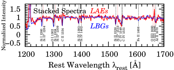
Moreover, recent NIR spectroscopy by Nakajima et al. [46] has suggested that LAEs have a large O iiiO ii ratio, indicating these systems are highly ionized with density-bounded H ii regions. This tendency has been confirmed by a subsequent systematic study in Nakajima & Ouchi [45]. The large O iiiO ii ratio also indicates a low column density of H i gas. A stacked UV continuum spectrum of our eight LAEs shows that LIS absorption lines have a low EW, as shown in Figures 15 (see also Fig. 11). The weak LIS absorption lines are consistent with a large O iiiO ii ratio in LAEs [29, e.g., ].
In our first paper of the series investigating LAE structures, we find that LAEs with a high Ly EW tend to be a non-merger, to show a small Ly spatial offset between Ly and stellar continuum emission , and to have a small ellipticity by using a large sample of 426 LAEs [64]. On the basis of these results on the gas distribution, the difference in H i column density explains the Ly-EW dependences of the merger fraction, the Ly spatial offset, and the galaxy inclination. For objects with density-bounded H ii regions, Ly photons would directly escape from central ionizing sources, which produce a small . The low H i abundance along the line of sight also induces the preferential escape of Ly to the face-on direction.
All of the above results suggest that ionized regions with small amounts of H i gas dominate in galaxies with a high Ly.
VIII. SUMMARY and CONCLUSION
We carry out deep optical spectroscopy for our large sample of LAEs at in order to detect their Ly lines with Keck/LRIS. We compare redshifts of the Ly and nebular emission lines detected with Subaru/FMOS, and calculate for new 11 LAEs. This observation doubles the sample size of LAEs with a measurement in literatures.
The conclusions of this study are summarized below.
- •
Almost all of our new LAEs have a of km s-1 which is systematically-smaller than that of LBGs. Using 22 LAEs with measurements taken from our new observations and the literature, we definitively confirm the anti-correlation between Ly EW and suggested by previous work.
- •
Long exposure times and the high sensitivity of LRIS at blue wavelengths enabled us to successfully detect IS absorption lines against faint UV continua from four individual LAEs. These IS absorption lines are found to be blueshifted from the systemic redshift by km s-1, indicating strong gaseous outflows are present even in LAEs.
- •
We estimate () that would be a quantity sensitive to for the four UV continuum-detected LAEs. We find the value of in LAEs to be smaller than that of LBGs, indicating a lower in LAEs. We performed a test for correlations between and physical properties inferred from SED fitting. As a result, we tentatively conclude that SFR may be most closely related to . The correlation may suggest that the star formation preferentially occurs in systems with large amounts of neutral hydrogen gas, which would have a larger value of .
- •
We estimate the covering fraction, , of surrounding H i gas from the depth of LIS absorption lines the four LAEs. We identify a tentative trend for to decrease with increasing Ly EW, as suggested by a study for LBGs in Jones et al. [30]. A central source being covered by patchy H i gas clouds would lead to a small flux-averaged corresponding to a small . In this condition, Ly photons could easily escape less affected by resonant scattering in the clouds.
- •
The results of our kinematic analyses support the idea that the H i column density is a key quantity determining Ly emissivity.
In this kinematic study, we obtain , , and only for objects with a moderate Ly EW of Å which overlaps with the Ly EW range of LBG samples in e.g., Shapley et al. [62]. We need to estimate these quantities for objects with a higher Ly EW in order to check whether such objects follow the kinematic trends found in this study.
References
- [1] Behrens, C., Dijkstra, M., & Niemeyer, J. C. 2014, A&A, 563, A77
- [2] Bruzual, G., & Charlot, S. 2003, MNRAS, 344, 1000
- [3] Calzetti, D., Armus, L., Bohlin, R. C., Kinney, A. L., Koornneef, J., & Storchi-Bergmann, T. 2000, ApJ, 533, 682
- [4] Chabrier, G. 2003, PASP, 115, 763
- [5] Chonis, T. S., et al. 2013, ApJ, 775, 99
- [6] Christensen, L., et al. 2012, MNRAS, 427, 1973
- [7] Ciardullo, R., et al. 2012, ApJ, 744, 110
- [8] Cowie, L. L., Barger, A. J., & Hu, E. M. 2010, ApJ, 711, 928
- [9] Dijkstra, M., & Kramer, R. 2012, MNRAS, 424, 1672
- [10] Dijkstra, M., & Wyithe, J. S. B. 2010, MNRAS, 408, 352
- [11] Dressler, A., Martin, C. L., Henry, A., Sawicki, M., & McCarthy, P. 2011, ApJ, 740, 71
- [12] Duval, F., Schaerer, D., Östlin, G., & Laursen, P. 2013, ArXiv e-prints
- [13] Erb, D. K., Pettini, M., Shapley, A. E., Steidel, C. C., Law, D. R., & Reddy, N. A. 2010, ApJ, 719, 1168
- [14] Erb, D. K., Steidel, C. C., Shapley, A. E., Pettini, M., Reddy, N. A., & Adelberger, K. L. 2006a, ApJ, 647, 128
- [15] —. 2006b, ApJ, 646, 107
- [16] Finkelstein, S. L., Rhoads, J. E., Malhotra, S., Grogin, N., & Wang, J. 2008, ApJ, 678, 655
- [17] Finkelstein, S. L., Rhoads, J. E., Malhotra, S., Pirzkal, N., & Wang, J. 2007, ApJ, 660, 1023
- [18] Finkelstein, S. L., et al. 2011, ApJ, 729, 140
- [19] Furusawa, H., et al. 2008, ApJS, 176, 1
- [20] Gawiser, E., et al. 2007, ApJ, 671, 278
- [21] Giacconi, R., et al. 2001, ApJ, 551, 624
- [22] Giavalisco, M., et al. 2004, ApJ, 600, L93
- [23] Gronwall, C., Bond, N. A., Ciardullo, R., Gawiser, E., Altmann, M., Blanc, G. A., & Feldmeier, J. J. 2011, ApJ, 743, 9
- [24] Gronwall, C., et al. 2007, ApJ, 667, 79
- [25] Guaita, L., Francke, H., Gawiser, E., Bauer, F. E., Hayes, M., Östlin, G., & Padilla, N. 2013, A&A, 551, A93
- [26] Guaita, L., et al. 2011, ApJ, 733, 114
- [27] Hashimoto, T., Ouchi, M., Shimasaku, K., Ono, Y., Nakajima, K., Rauch, M., Lee, J., & Okamura, S. 2013, ApJ, 765, 70
- [28] Hu, E. M., Cowie, L. L., Barger, A. J., Capak, P., Kakazu, Y., & Trouille, L. 2010, ApJ, 725, 394
- [29] Jones, T., Stark, D. P., & Ellis, R. S. 2012, ApJ, 751, 51
- [30] Jones, T. A., Ellis, R. S., Schenker, M. A., & Stark, D. P. 2013, ApJ, 779, 52
- [31] Kashikawa, N., et al. 2006, ApJ, 648, 7
- [32] —. 2011, ApJ, 734, 119
- [33] Kennicutt, Jr., R. C. 1998, ARA&A, 36, 189
- [34] Kimura, M., et al. 2010, PASJ, 62, 1135
- [35] Komatsu, E., et al. 2011, ApJS, 192, 18
- [36] Kulas, K. R., Shapley, A. E., Kollmeier, J. A., Zheng, Z., Steidel, C. C., & Hainline, K. N. 2012, ApJ, 745, 33
- [37] Laursen, P., Duval, F., & Östlin, G. 2013, ApJ, 766, 124
- [38] Laursen, P., & Sommer-Larsen, J. 2007, ApJ, 657, L69
- [39] Laursen, P., Sommer-Larsen, J., & Andersen, A. C. 2009, ApJ, 704, 1640
- [40] Madau, P. 1995, ApJ, 441, 18
- [41] McCracken, H. J., et al. 2010, ApJ, 708, 202
- [42] McLinden, E. M., et al. 2011, ApJ, 730, 136
- [43] Miyazaki, S., et al. 2002, PASJ, 54, 833
- [44] Momose, R., et al. 2014, ArXiv e-prints
- [45] Nakajima, K., & Ouchi, M. 2013, ArXiv e-prints
- [46] Nakajima, K., Ouchi, M., Shimasaku, K., Hashimoto, T., Ono, Y., & Lee, J. C. 2013, ApJ, 769, 3
- [47] Nakajima, K., et al. 2012, ApJ, 745, 12
- [48] Neufeld, D. A. 1991, ApJ, 370, L85
- [49] Oke, J. B., & Gunn, J. E. 1983, ApJ, 266, 713
- [50] Oke, J. B., et al. 1995, PASP, 107, 375
- [51] Ono, Y., et al. 2010, MNRAS, 402, 1580
- [52] Ota, K., et al. 2008, ApJ, 677, 12
- [53] Ouchi, M., et al. 2008, ApJS, 176, 301
- [54] —. 2010, ApJ, 723, 869
- [55] Pettini, M., Shapley, A. E., Steidel, C. C., Cuby, J.-G., Dickinson, M., Moorwood, A. F. M., Adelberger, K. L., & Giavalisco, M. 2001, ApJ, 554, 981
- [56] Rauch, M., et al. 2008, ApJ, 681, 856
- [57] Reddy, N. A., Steidel, C. C., Pettini, M., Adelberger, K. L., Shapley, A. E., Erb, D. K., & Dickinson, M. 2008, ApJS, 175, 48
- [58] Rhoads, J. E., Malhotra, S., Richardson, M. L. A., Finkelstein, S. L., Fynbo, J. P. U., McLinden, E. M., & Tilvi, V. S. 2014, ApJ, 780, 20
- [59] Schaerer, D., & de Barros, S. 2009, A&A, 502, 423
- [60] Schenker, M. A., Ellis, R. S., Konidaris, N. P., & Stark, D. P. 2013, ApJ, 777, 67
- [61] Scoville, N., et al. 2007, ApJS, 172, 1
- [62] Shapley, A. E., Steidel, C. C., Pettini, M., & Adelberger, K. L. 2003, ApJ, 588, 65
- [63] Shibuya, T., Kashikawa, N., Ota, K., Iye, M., Ouchi, M., Furusawa, H., Shimasaku, K., & Hattori, T. 2012, ApJ, 752, 114
- [64] Shibuya, T., Ouchi, M., Nakajima, K., Yuma, S., Hashimoto, T., Shimasaku, K., Mori, M., & Umemura, M. 2014, ApJ, 785, 64
- [65] Steidel, C. C., Adelberger, K. L., Shapley, A. E., Pettini, M., Dickinson, M., & Giavalisco, M. 2000, ApJ, 532, 170
- [66] Steidel, C. C., Erb, D. K., Shapley, A. E., Pettini, M., Reddy, N., Bogosavljević, M., Rudie, G. C., & Rakic, O. 2010, ApJ, 717, 289
- [67] Steidel, C. C., Shapley, A. E., Pettini, M., Adelberger, K. L., Erb, D. K., Reddy, N. A., & Hunt, M. P. 2004, ApJ, 604, 534
- [68] Verhamme, A., Schaerer, D., Atek, H., & Tapken, C. 2008, A&A, 491, 89
- [69] Verhamme, A., Schaerer, D., & Maselli, A. 2006, A&A, 460, 397
- [70] Yajima, H., Li, Y., Zhu, Q., Abel, T., Gronwall, C., & Ciardullo, R. 2012, ArXiv e-prints
- [71] Zheng, Z., Cen, R., Trac, H., & Miralda-Escudé, J. 2010, ApJ, 716, 574
- [72] Zheng, Z., & Wallace, J. 2013, ArXiv e-prints