Lagrangian ADER-WENO Finite Volume Schemes on Unstructured Tetrahedral Meshes for Conservative and Nonconservative Hyperbolic Systems in 3D
Abstract
In this paper we present a new family of high order accurate Arbitrary-Lagrangian-Eulerian (ALE) one-step ADER-WENO finite volume schemes for the solution of nonlinear systems of conservative and non-conservative hyperbolic partial differential equations with stiff source terms on moving tetrahedral meshes in three space dimensions. A WENO reconstruction technique is used to achieve high order of accuracy in space, while an element-local space-time Discontinuous Galerkin finite element predictor on moving meshes is used to obtain a high order accurate one-step time discretization. Within the space-time predictor the physical element is mapped onto a reference element using an isoparametric approach, where the space-time basis and test functions are given by the Lagrange interpolation polynomials passing through a predefined set of space-time nodes. Since our algorithm is cell-centered, the final mesh motion is computed by using a suitable node solver algorithm. A rezoning step as well as a flattener strategy are used in some of the test problems to avoid mesh tangling or excessive element deformations that may occur when the computation involves strong shocks or shear waves. The ALE algorithm presented in this article belongs to the so-called direct ALE methods because the final Lagrangian finite volume scheme is based directly on a space-time conservation formulation of the governing PDE system, with the rezoned geometry taken already into account during the computation of the fluxes.
We apply our new high order unstructured ALE schemes to the 3D Euler equations of compressible gas dynamics, for which a set of classical numerical test problems has been solved and for which convergence rates up to sixth order of accuracy in space and time have been obtained. We furthermore consider the equations of classical ideal magnetohydrodynamics (MHD) as well as the non-conservative seven-equation Baer-Nunziato model of compressible multi-phase flows with stiff relaxation source terms.
Keywords:
Arbitrary-Lagrangian-Eulerian (ALE) finite volume schemes , WENO reconstruction on moving unstructured tetrahedral meshes , high order of accuracy in space and time , stiff source terms , local rezoning , conservation laws and nonconservative hyperbolic PDE , Euler equations , MHD equations , compressible multi-phase flows , Baer-Nunziato model1 Introduction
Any Lagrangian method aims at following the fluid motion as closely as possible, with a computational mesh that is moving with the local fluid velocity. Therefore the Lagrangian approach allows material interfaces and contact waves to be precisely located and tracked during the computation, achieving a much more accurate resolution of these waves compared to classical Eulerian methods on fixed grids. For this reason a lot of research has been carried out in the last decades in order to develop Lagrangian methods. Already John von Neumann and Richtmyer were working on Lagrangian schemes in the 1950ies [118], using a formulation of the governing equations in primitive variables, which was also used later in [8, 18]. However, most of the modern Lagrangian finite volume schemes use the conservation form of the equations based on the physically conserved quantities like mass, momentum and total energy in order to compute shock waves properly, see e.g. [93, 108, 89, 20]. Lagrangian schemes can be also classified according to the location of the physical variables on the mesh: when all variables are defined on a collocated grid the so-called cell-centered approach is adopted [31, 102, 89, 90, 88], while in the staggered mesh approach [84, 85] the velocity is defined at the cell interfaces and the other variables at the cell center.
Cell-centered Lagrangian Godunov-type schemes of the Roe-type and of the HLL-type for the Euler equations of compressible gas dynamics have first been considered by Munz in [93]. A cell-centered Godunov-type scheme has also been introduced by Carré et al. in [20], who developed a Lagrangian finite volume algorithm on general multi-dimensional unstructured meshes. The resulting finite volume scheme is node based and compatible with the mesh displacement. In the work of Després et al. [35, 36] the physical part of the system of equations is coupled and evolved together with the geometrical part, hence obtaining a weakly hyperbolic system of conservation laws that is solved using a node-based finite volume scheme. Furthermore they presented a cell-centered Lagrangian method [31] that is translation invariant and suitable for curved meshes. In [86, 88, 87] Maire proposed first and second order accurate cell-centered Lagrangian schemes in two- and three- space dimensions on general polygonal grids, where the time derivatives of the fluxes are obtained using a node-centered solver that may be considered as a multi-dimensional extension of the Generalized Riemann problem methodology introduced by Ben-Artzi and Falcovitz [7], Le Floch et al. [61, 16] and Titarev and Toro [113, 110, 111]. The node solver algorithm developed for hydrodynamics by Maire in [86] is used also in this paper and applied to both Euler and MHD equations on moving tetrahedral meshes. Since Lagrangian schemes may lead to severe mesh deformation after a finite time, it is necessary to remesh (or at least to rezone) the computational grid from time to time. A very popular approach consists therefore in Lagrangian remesh and remap schemes, such as the family of cell-centered ALE remap algorithms introduced by Shashkov et al. and Maire et al. in [102, 11, 79, 81, 78, 9]. In [62, 119, 17, 103] purely Lagrangian and Arbitrary-Lagrangian-Eulerian (ALE) numerical schemes with remapping for multi-phase and multi-material flows are discussed. All the Lagrangian schemes listed so far are at most second order accurate in space and time.
Higher order of accuracy in space was first achieved in [26, 82, 27, 28] by Cheng and Shu, who introduced a third order accurate essentially non-oscillatory (ENO) reconstruction operator into Godunov-type Lagrangian finite volume schemes. High order of accuracy in time was guaranteed either by the use of a Runge-Kutta or by a Lax-Wendroff-type time stepping. The mesh velocity is simply computed as the arithmetic average of the corner-extrapolated values in the cells adjacent to a mesh vertex. Such a node solver algorithm is very simple and general and can be easily applied to different complicated nonlinear systems of hyperbolic PDE in multiple space dimensions. Cheng and Toro [29] also investigated Lagrangian ADER-WENO schemes in one space dimension. In the finite element framework high order Lagrangian schemes have been developed for example by Scovazzi et al. [95, 107]. In [53] Dumbser et al. presented high order ADER-WENO Lagrangian finite volume schemes for hyperbolic balance laws with stiff source terms. In this case the high order of accuracy in time was achieved by using the local space-time Galerkin predictor method proposed in [46, 67] for the Eulerian case, whereas a high order WENO reconstruction algorithm was used to obtain high order of accuracy in space. In [13, 44] Boscheri and Dumbser extended this algorithm to unstructured triangular meshes for conservative and non-conservative hyperbolic systems with stiff source terms. In [14] three different node solver algorithms have been applied to the Euler equations of compressible gas dynamics as well as to the equations for magnetohydrodynamics and have been compared with each other. The multidimensional HLL Riemann solver presented in [38] for the Eulerian framework on fixed grids has been used as a node solver for the computation of the mesh velocity in [14] and for the computation of the space-time fluxes of a high order Lagrangian finite volume scheme in [12]. In the latter reference it has been shown that the use of a multi-dimensional Riemann solver allows the use of larger time steps in multiple space dimensions and therefore leads to a computationally more efficient scheme compared to a method based on classical one-dimensional Riemann solvers.
In literature there are also other methods using a Lagrangian approach and these schemes are at least briefly mentioned in the following. For example, also meshless particle schemes, such as the smooth particle hydrodynamics (SPH) method, belong to the category of fully Lagrangian schemes, see e.g. [92, 58, 57, 59, 60]. SPH is generally used to follow the fluid motion in very complex deforming domains. Since it is a particle method, no rezoning or remeshing has to be applied. Furthermore, also semi-Lagrangian methods should be mentioned. They are typically adopted to solve transport equations [101, 66]. Although these schemes use a fixed mesh, as in the classical Eulerian approach, the Lagrangian trajectories of the fluid are followed backward in time in order to compute the numerical solution at the the new time level, see for example [23, 24, 80, 70, 99, 15]. There is also the class of Arbitrary-Lagrangian-Eulerian (ALE) methods [68, 98, 108, 39, 56, 55, 25], where the mesh moves with a velocity that does not necessarily have to coincide with the local fluid velocity. This method is often used for fluid-structure interaction (FSI) problems, but it is also used together with Lagrangian remap schemes. For the sake of generality, the scheme presented in this article uses an ALE approach so that the local mesh velocity can in principle be chosen independently from the local fluid velocity.
In this paper we extend the algorithm presented in [13, 44] to moving unstructured tetrahedral meshes in three space dimensions. To the knowledge of the authors, this is the first better than second order accurate Lagrangian finite volume method on three-dimensional tetrahedral meshes ever presented. We consider the Euler equations of compressible gas dynamics as well as the ideal classical MHD equations and the non-conservative seven-equation Baer-Nunziato model of compressible multi-phase flows with stiff source terms. The node solver proposed by Maire in [86] is applied, as well as the node solver of Cheng and Shu [26].
The rest of this article is structured as follows: in Section 2 we describe the proposed numerical scheme in detail, while in Section 3 we show numerical convergence studies up to sixth order of accuracy in space and time as well as numerical results for several classical test problems for all of the above-mentioned hyperbolic systems. Finally, in Section 4 we give some concluding remarks and an outlook to future research and developments.
2 Numerical method
In this paper we consider nonlinear systems of hyperbolic balance laws which may also contain non-conservative products and stiff source terms. A general formulation that is suitable to write the above mentioned systems reads
| (1) |
where denotes the vector of conserved variables, is the conservative nonlinear flux tensor, contains the purely non-conservative part of the system written in block-matrix notation and represents a nonlinear algebraic source term that is allowed to be stiff. We furthermore introduce the abbreviation to ease notation in some parts of the manuscript.
In a Lagrangian framework the computational domain is time-dependent and is discretized at the current time by a set of tetrahedral elements . denotes the total number of elements contained in the domain and the union of all elements is called the current tetrahedrization of the domain
| (2) |
Since we are dealing with a moving computational domain where the mesh configuration continuously changes in time, it is more convenient to map the physical element to a reference element via a local reference coordinate system . The spatial reference element is the unit tetrahedron shown in Figure 1 and is defined by the nodes , , and , where is the vector of the spatial coordinates in the reference system, while the position vector is defined in the physical system. Let furthermore be the vector of physical spatial coordinates of the -th vertex of tetrahedron . Then the linear mapping from to is given by
| (3) |
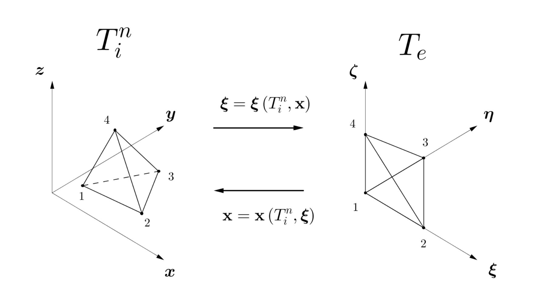
As usual for finite volume schemes, data are stored and evolved in time as piecewise constant cell averages. They are defined at each time level within the control volume as
| (4) |
with denoting the volume of tetrahedron . In the next Section 2.1 a WENO reconstruction technique is described and used to obtain piecewise higher order polynomials from the known cell averages . High order of accuracy in time is achieved later in Section 2.2 by applying a local space-time Galerkin predictor method to the reconstruction polynomials .
2.1 Polynomial WENO reconstruction
The WENO reconstruction operator produces piecewise polynomials of degree . The are computed for each control volume from the known cell averages within a so-called reconstruction stencil , which is composed of an appropriate neighborhood of element and contains a prescribed total number of tetrahedra. We do not use the original pointwise WENO method first introduced by Shu et al. [71, 69, 120], but we adopt the polynomial formulation proposed in [63, 75, 48, 49] and also used in [112, 117], which is relatively simple to code and which allows the scheme to reach very high order of accuracy even on unstructured tetrahedral meshes in three space dimensions.
According to [49], in three space dimensions we always use nine reconstruction stencils, hence . Specifically, we consider one central stencil given by , four forward stencils with and four backward stencils with , as depicted in Figure 2. Each forward and backward stencil sector is spanned by one point and three vectors: the four forward stencils are defined by a vertex of the tetrahedron and the triplet of vectors connecting to the three vertices of the opposite face, while the backward sectors are defined by the negative vectors of the forward stencils and the opposite face barycenter. Each type of stencil is filled by recursively adding neighbor elements until the prescribed total number is reached. An element belongs to the stencil if its barycenter is located in the corresponding sector. For the central stencil we use a simple Neumann-type neighbor search algorithm that recursively adds direct face neighbors to the stencil, until the desired number is reached. For the remaining eight one-sided stencils we use a Voronoi-type search algorithm, which fills the stencil starting from the vertex neighborhood of the tetrahedron and then using recursively vertex neighbors of stencil elements. Each stencil contains a total number of elements that depends on the reconstruction degree , hence
| (5) |
where is a local index which progressively counts the elements in the stencil number and represents a mapping from the local index to the global index of the element in . As explained in [6, 94, 75], the total number of elements must be greater than the smallest number needed to reach the formal order of accuracy . As suggested in [49, 48] we typically take in three space dimensions.
The high order reconstruction polynomial for each candidate stencil for tetrahedron is written in terms of the orthogonal Dubiner-type basis functions [40, 74, 32] on the reference tetrahedron , i.e.
| (6) |
where the mapping to the reference coordinate system is given by (3) and denote the unknown degrees of freedom (expansion coefficients) of the reconstruction polynomial on stencil for element at time . In the rest of the paper we will use classical tensor index notation based on the Einstein summation convention, which implies summation over two equal indices.
Integral conservation is required for the reconstruction on each element of the stencil , hence
| (7) |
Inserting the transformation (3) into the above expression (7), an analytical integration formula can be obtained that is a function of the four physical vertex coordinates of the tetrahedron. The resulting algebraic expressions of the integrals appearing in (7) can be obtained for example at the aid of a symbolic computer algebra system like MAPLE. Up to we use the aforementioned analytical integration, while for higher reconstruction degrees the integrals in (7) are simply evaluated using Gaussian quadrature formulae of suitable order, see [109] for details, since the analytical expressions become too cumbersome. The reconstruction matrix, which is given by the integrals of the linear system (7), depends on the geometry of the tetrahedral elements in stencil . Therefore, since in the Lagrangian framework the mesh is moving in time the reconstruction matrix can not be inverted and stored once and for all during a preprocessing stage, like in the Eulerian case. As a consequence, we assemble and solve the small reconstruction system (7) for each element directly at the beginning of each time step using optimized LAPACK subroutines. This makes the Lagrangian WENO reconstruction computationally more expensive but at the same time also much less memory consuming compared to the original Eulerian WENO algorithm presented in [49, 48], since no reconstruction matrices are stored.
While the mesh is moving in time, we always assume that the connectivity of the mesh and therefore also the topology of each reconstruction stencil remains constant in time. Therefore, the definition of the stencils does not need to be updated during the simulation. This is a very important simplification, since the stencil search may be quite time consuming in three space dimensions.
Since each stencil is filled with a total number of elements, system (7) results in an overdetermined linear system that has to be solved properly by either using a constrained least-squares technique (LSQ), see [49], or a more sophisticated singular value decomposition (SVD) algorithm. In order to avoid ill-conditioned reconstruction matrices, see [1], each element in a stencil is first mapped to the reference coordinate system associated with element by using the transformation (3) before solving (7).
 |
 |
 |
As stated by the Godunov theorem [65], linear monotone schemes are at most of order one and if the scheme is required to be higher order accurate and non-oscillatory, it must be nonlinear. Therefore a nonlinear formulation has to be used for the final WENO reconstruction polynomial. We first measure the smoothness of each reconstruction polynomial obtained on stencil by a so-called oscillation indicator [71],
| (8) |
which is computed on the reference element using the (universal) oscillation indicator matrix , which, according to [49], is given by
| (9) |
The nonlinearity is then introduced into the scheme by the WENO weights , which read
| (10) |
with the parameters and . According to [49] the linear weights are chosen as for the central stencil and for the one-sided stencils (). Formula (10) is intended to be read componentwise. For a WENO reconstruction based on characteristic variables see [48]. A weighted nonlinear combination of the reconstruction polynomials obtained on each candidate stencil yields the final WENO reconstruction polynomial and its coefficients:
| (11) |
Positivity preserving technique.
Several phenomena in physics and engineering as well as many classical benchmark test cases in the Lagrangian framework are involving strong shock waves, which may lead to a loss of positivity for density and pressure in the numerical scheme. Such a problem typically occurs after carrying out the high-order reconstruction algorithm presented in Section 2.1, which is designed to be essentially but not absolutely non-oscillatory. For this reason we rely on the positivity preserving technique of Balsara [5], where a flattener variable is computed in order to smear out the oscillations and to bring back density and pressure values to their physically admissible range if the positivity constraint has been violated. In [5] the equations for both hydrodynamics and magnetohydrodynamics have been considered on two- and three-dimensional Cartesian grids and in this paper we extend the method to moving unstructured tetrahedral meshes.
First we have to detect those regions of the computational domain which are characterized by strong shocks. Let us consider a tetrahedron and its Neumann neighborhood , i.e. all the elements that are attached to a face of . Let furthermore and be the vectors of conserved variables of element and its direct neighbor , respectively, and let denote the density and the pressure. A shock can be identified by comparing the divergence of the velocity field with the minimum of the sound speed obtained by considering the element itself as well as its neighborhood . Hence,
| (12) |
where represents as usual the volume of the tetrahedron , denotes the surface shared between element and the neighbor , is the associated unit normal vector w.r.t. the surface and are the sound speeds of and the neighbor element , respectively, with representing the ratio of specific heats. The divergence of the velocity field is estimated from the cell-averaged states and not from the reconstructed states obtained from (11).
The flattener variable is then computed according to [5] as
| (13) |
with the coefficient that is set to the value of for all our computations. For rarefaction waves the divergence of the velocity field is positive, i.e. , hence obtaining and leaving the reconstruction polynomial as it is. Even when shocks of modest strength occur, i.e. , the reconstruction remains untouched.
In the work of Balsara [5] the flattener variable is propagated even to those elements that are about to be crossed by a shock, but have still to enter the wave, i.e. the neighbors of an element which has already experienced the shock. Due to the more complex computational domain on unstructured meshes, we propose to define a node based flattener : the Voronoi neighborhood of each vertex of element is also considered in order to propagate the flattener, hence taking into account all those elements that share vertex of tetrahedron . The node based flattener results in the maximum value among the flattener values of the attached tetrahedra that has been previously computed according to (13):
| (14) |
Each element is then assigned again with the maximum value of the node based flattener among the set of the four vertices that define the tetrahedron , i.e.
| (15) |
Once the flattener variable has been computed for each element of the computational domain , the WENO reconstruction polynomials are corrected with the following expression:
| (16) |
If positivity is still violated even after using (16), then is set, thus recovering a (positivity preserving) first order finite volume scheme. This strategy resembles to some extent the recently developed MOOD algorithm of Diot et al. [30, 37, 83], however, it is still used as an a priori limiter here, while the MOOD approach uses an innovative a posteriori limiting philosophy. The development of high order Lagrangian MOOD schemes will be the topic of future research. The presented flattener technique is by default switched off and has been used only for those test problems where it was absolutely necessary in order to run the simulation to the final time. We therefore explicitly state in Section 3 if the flattener has been used.
2.2 Local space-time Discontinuous Galerkin predictor on moving curved tetrahedra
The reconstructed polynomials computed at the current time are then evolved during one time step locally within each element without requiring any neighbor information. As a result, one obtains piecewise space-time polynomials of degree , denoted by . This allows the scheme to achieve also high order of accuracy in time. For this purpose an element-local weak space-time formulation of the governing PDE (1) is used. This approach has first been developed in the Eulerian framework on fixed grids by Dumbser et al. in [46, 43, 47, 67]. Later, it has been extended to the Lagrangian framework on moving grids in 1D and 2D in [53, 13, 44]. Here, we extend this approach for the first time to moving tetrahedral meshes in 3D. As already done in the past [46, 67, 54] we use the local space-time Discontinuous Galerkin predictor method, since it is able to handle also stiff source terms.
Let and be the spatial coordinate vectors defined in the physical and in the reference system, respectively, and let and be the corresponding space-time coordinate vectors. Let furthermore be a space-time basis function defined by the Lagrange interpolation polynomials passing through the space-time nodes , which are defined by the tensor product of the spatial nodes of classical conforming high order finite elements and the Gauss-Legendre quadrature points in time.
Since the Lagrange interpolation polynomials define a nodal basis, the functions satisfy the following interpolation property:
| (17) |
where denotes the usual Kronecker symbol. According to [43] the local solution , the fluxes , the source term and the non-conservative product are approximated within the space-time element with
| (18) |
Because of the interpolation property (17) we evaluate the degrees of freedom for , and in a pointwise manner from as
| (19) |
The degrees of freedom represent the gradient of in node .
An isoparametric approach is used, where the mapping between the physical space-time coordinate vector and the reference space-time coordinate vector is represented by the same basis functions used for the discrete solution itself. Therefore
| (20) |
where are the degrees of freedom of the spatial physical coordinates of the moving space-time control volume, which are unknown, while denote the known degrees of freedom of the physical time at each space-time node . The mapping in time is linear and simply reads
| (21) |
where represents the current time and is the current time step, which is computed under a classical Courant-Friedrichs-Levy number (CFL) stability condition, i.e.
| (22) |
with denoting the insphere diameter of tetrahedron and corresponding to the maximum absolute value of the eigenvalues computed from the solution in . On unstructured three-dimensional meshes the CFL stability condition must satisfy the inequality .
The Jacobian of the transformation from the physical space-time element to the reference space-time element reads
| (23) |
and its inverse is given by
| (24) |
We point out that in the Jacobian matrix and , as can be easily derived from the time mapping (21).
In the following we introduce the notation adopted for the nabla operator in the reference space and in the physical space :
| (25) |
and let us furthermore introduce the two integral operators
| (26) |
that denote the scalar products of two functions and over the spatial reference element at time and over the space-time reference element , respectively.
The governing PDE (1) is then reformulated in the reference coordinate system using the inverse of the associated Jacobian matrix (24) with and according to (21) and adopting the gradient notation illustrated in (25) above:
| (27) |
By introducing the following abbreviation
| (28) |
Eqn. (27) simplifies to
| (29) |
The numerical approximation of is computed by the same isoparametric approach used in (18) for the solution and the flux representation, i.e.
| (30) |
Inserting (18) and (30) into (27), then multiplying Eqn. (27) with the space-time test functions and integrating the resulting equation over the space-time reference element , one obtains a weak formulation of the governing PDE (1):
The term on the left hand side can be integrated by parts in time, yielding
| (31) |
where the initial condition of the local Cauchy problem has been introduced in a weak form.
Adopting the following more compact matrix-vector notation
| (32) |
the system (31) is reformulated as
| (33) |
Eqn. (33) constitutes an element-local nonlinear algebraic equation system for the unknown space-time expansion coefficients which can be solved using the following iterative scheme
| (34) |
where denotes the iteration number. In case of stiff algebraic source terms, the discretization of must be implicit, see [46, 54, 67, 53]. For an efficient initial guess of this iterative procedure in the case of stiff source terms see [67].
Together with the solution, we also have to evolve in time the geometry of the space-time control volume, i.e. the vertex coordinates of element , whose motion is described by the ODE system
| (35) |
with denoting the local mesh velocity. In this paper we are developing an Arbitrary-Lagrangian-Eulerian (ALE) method, which allows the mesh velocity to be chosen independently from the fluid velocity, so that the scheme may reduce either to a pure Eulerian approach in the case where or to a fully Lagrangian-type algorithm if coincides with the local fluid velocity . Any other choice for the mesh velocity is possible. The velocity inside element is also expressed in terms of the space-time basis functions as
| (36) |
with .
The local space-time DG method is used again to solve Eqn.(35) for the unknown coordinate vector , according to [53, 13, 44], hence
| (37) |
where is given by the mapping (3) based on the known vertex coordinates of tetrahedron at time . The above expression is then solved by an iterative procedure together with Eqn. (34) until the residuals of the predicted solution given by (34) and the new vertex position at iteration are less than a prescribed tolerance, typically set to .
Once we have carried out the above procedure for all the elements of the computational domain, we end up with an element-local predictor for the numerical solution , for the fluxes , for the source term and also for the mesh velocity .
Then we have to update the mesh globally, by assigning a unique velocity vector to each node, since we do not admit discontinuities in the geometry. In the next Section 2.3 a local node solver algorithm for the velocity together with a rezoning algorithm will be presented in detail, in order to obtain a uniquely defined vertex location at the new time level .
2.3 Mesh motion
Lagrangian schemes have been designed and developed in order to compute the flow variables by moving together with the fluid. As a consequence, the computational mesh continuously changes its configuration in time, following as closely as possible the flow motion. The mesh velocity plays indeed an important role and should be evaluated very accurately using a node solver algorithm, which assigns a velocity vector to each vertex of the mesh. A comparison between different node solver techniques can be found in [14]. Moreover, the flow motion may become very complex, hence highly deforming the computational elements, that are compressed, twisted or even tangled. Therefore, the challenge of any Lagrangian scheme is to preserve at the same time the excellent resolution properties of contact waves and material interfaces together with a good mesh quality without invalid elements. A suitable rezoning algorithm [77] is typically used to improve the mesh quality together with a so-called relaxation algorithm [64] to partially recover the optimal Lagrangian accuracy where the computational elements are not distorted too much. In the following we present in detail the three main steps adopted in our ADER-WENO ALE finite volume schemes to move the mesh vertices to the final mesh configuration at the new time level : the Lagrangian step, the rezoning step and the relaxation step.
2.3.1 The Lagrangian step.
At the end of the local predictor procedure illustrated in Section 2.2, each vertex is assigned with several velocity vectors , each of them coming from the Voronoi neighborhood which is composed by the neighbor elements that share the common node . Moving the same vertex to the next time level with different velocities would lead to a discontinuity in the geometry, that is not admissible in our Lagrangian algorithm. Therefore a node solver technique is adopted in order to fix a unique velocity for each node of the computational grid. In [14] Boscheri et al. compare three different node solvers for unstructured triangular meshes with each other and here we extend two of them to the three-dimensional case, in particular the node solver of Cheng and Shu and the node solver of Maire.
Let be the Voronoi neighborhood of vertex , that is composed by a total number of neighbor elements denoted by , and let furthermore represent a mapping from the global node number defined in to the local vertex number in element . The local velocity computed within element is evaluated as the time integral of the high order vertex-extrapolated velocity at node , i.e.
| (38) |
The node solver computes the velocity of vertex as a mass weighted average velocity among its neighborhood and it reads
| (39) |
where the local weights are defined as the product between the cell averaged value of density and the cell volume , hence
| (40) |
In [86, 88, 87] Maire et al. developed the node solver for hydrodynamics, while in [20] Després presented a similar approach. All the details can be found in the above-mentioned references, hence we limit us here only to a brief overview of this node solver algorithm, which is based on the conservation of total energy in the equations for compressible hydrodynamics. According to Figure 3, is the node index, denotes the neighbor element of vertex and the subscripts represent the three faces of tetrahedron which share node , ordered adopting a counterclockwise convention. Furthermore are assumed to be one third of the corresponding face areas and denote the associated outward pointing unit normal vectors. Finally is the fluid pressure and is the speed of sound for hydrodynamics.

The total energy at the generic node is conserved only if the sum of the forces acting on node is zero, i.e.
| (41) |
In (41) the sub-cell force exerted by each neighbor element onto vertex , is evaluated solving approximately three half Riemann problems on the faces . The acoustic Riemann solver of Dukowicz et al. [42] is used to obtain the final expression for the sub-cell force, which reads
| (42) |
with denoting the corner vector related to node . represents the known vertex velocity of cell according to (38), while denotes the unknown velocity of node . is a symmetric positive definite matrix that is evaluated as
| (43) |
where is the acoustic impedance. The equation for the total energy conservation (41) can be reformulated using the expression for the sub-cell force (42), hence obtaining a linear algebraic system for the unknown node velocity :
| (44) |
Since matrix is always invertible, this system admits a unique solution and the node velocity can always be evaluated. Instead of taking the above-defined acoustic impedance, one can compute it as originally proposed by Dukowicz in [42]:
| (45) |
where is a material dependent parameter which is a function of the ratio of specific heats . In this case the system (44) becomes nonlinear, due to the dependency of the acoustic impedance on the unknown node velocity, and a suitable iterative algorithm has to be used to obtain the solution.
Once a unique velocity has been defined for each node of the mesh, the new Lagrangian coordinates are computed as
| (46) |
with representing the coordinates of node at the current time level .
2.3.2 The rezoning step.
The Lagrangian step allows the nodes to follow the fluid motion as closely as possible. However, this may lead to bad quality elements, where the Jacobians become very small or even negative. This either drastically decreases the admissible timestep, according to (22), or even leads to a failure of the computation. Therefore, also a rezoned position should be computed for each node in order to improve the local mesh quality without taking into account any physical information. We use a different treatment for internal nodes and boundary nodes. Specifically, the rezoning algorithm presented in [77, 64] is adopted for inner nodes, while a variant of the feasible set method proposed by Berndt et al. [10] is used for the boundary nodes.
The rezoning algorithm aims at improving the mesh quality locally, i.e. in the Voronoi neighborhood of node considering all the neighbor elements , which for sake of simplicity will be addressed by . The starting point is the Lagrangian coordinate vector obtained at the end of the Lagrangian step. The rezoning procedure consists in optimizing a goal function that has to be defined for each node as
| (47) |
where is the condition number of the Jacobian matrix of the mapping from the reference tetrahedron to the physical element :
| (48) |
In (48) the coordinate vector represents the four nodes of the neighbor tetrahedron , which are counterclockwise ordered in such a way that node corresponds to . Then, the condition number of matrix is given by
| (49) |
The goal function is computed according to [77] as the sum of the local condition numbers of the neighbors, i.e.
| (50) |
and its minimization leads to a locally optimal position of the free node . As proposed in [64], the optimized rezoned coordinates for vertex are computed using the first step of a Newton algorithm, hence
| (51) |
where and represent the Hessian and the gradient of the goal function , respectively:
| (52) |
For the boundary nodes we present a simplified but very efficient version of the feasible set method proposed in [10] for two-dimensional unstructured meshes. The original feasible set method has been designed in order to find the convex polygon on which a vertex can lie without invalid elements in its neighborhood. In three space dimensions such an algorithm becomes very complex and high demanding in terms of computational efforts. In our simplified procedure the rezoned coordinates of the boundary node is evaluated as a volume weighted average among the barycenter coordinates of each neighbor element , which is
| (53) |
with the weights
| (54) |
and the barycenter defined as usual as
| (55) |
2.3.3 The relaxation step.
Since our ALE scheme is supposed to be as Lagrangian as possible, we do not want to rezone the mesh nodes where it is not strictly necessary in order to carry on the computation. Therefore the final node position is obtained applying the relaxation algorithm of Galera et al. [64], that performs a convex combination between the Lagrangian position and the rezoned position of node , hence
| (56) |
where is a node-based coefficient associated to the deformation of the Lagrangian grid over the time step . The values for are bounded in the interval , so that when a fully Lagrangian mesh motion occurs, while if the new node location is defined by the pure rezoned coordinates . We point out that the coefficient is designed to result in for rigid body motion, namely rigid translation and rigid rotation, where no element deformation occurs. Further details about the computation of can be found in [64].
2.4 Finite volume scheme
In order to develop a Lagrangian finite volume schemes on moving tetrahedra, we adopt the same approach used for our ALE algorithm in two space dimensions presented in [13, 44]. There, the governing PDE (1) is reformulated more compactly using a space-time divergence operator , hence obtaining
| (57) |
where the space-time flux tensor and the system matrix explicitly read
| (58) |
For the computation of the state vector at the new time level , the balance law (57) is integrated over a four-dimensional space-time control volume , i.e.
| (59) |
Application of the theorem of Gauss yields
| (60) |
where the space-time volume integral on the left of (59) has been rewritten as the sum of the fluxes computed over the three-dimensional space-time volume , given by the evolution of each face of element within the timestep , as depicted in Figure 4. The symbol denotes the outward pointing space-time unit normal vector on the space-time face .
Since the algorithm is required to deal with both, conservative and non-conservative hyperbolic systems, we use a path-conservative approach to integrate the non-conservative product, see [116, 97, 22, 21, 100, 45, 47, 52, 44]. One thus obtains
| (61) |
where a new term has been introduced in order to take into account potential jumps of the solution on the space-time element boundaries . This term is computed by the path integral
| (62) |
The integration path in (62) is chosen to be a simple straight-line segment [97, 22, 47, 52], although other choices are possible. Therefore it reads
| (63) |
and the jump term (62) simply reduces to
| (64) |
with representing the two vectors of conserved variables within element and its direct neighbor , respectively.
Let denote the Neumann neighborhood of tetrahedron , which is the set of directly adjacent neighbors that share a common face with tetrahedron . The space-time volume is composed by four space-time sub-volumes , each of them defined for each face of tetrahedron as depicted in Figure 4, and two more space-time sub-volumes, and , that represent the tetrahedron configuration at times and , respectively. Hence, the space-time volume involves overall a total number of six space-time sub-volumes, i.e.
| (65) |
Each of the space-time sub-volumes is mapped to a reference element in order to simplify the integral computation. For the configurations at the current and at the new time level, and , we use the mapping (3) with . The space-time unit normal vectors simply read for and for , since these volumes are orthogonal to the time coordinate. For the lateral sub-volumes we adopt a linear parametrization to map the physical volume to a four-dimensional space-time reference prism, as shown in Figure 4. Starting from the old vertex coordinates and the new ones , that are known from the mesh motion algorithm described in Section 2.3, the lateral sub-volumes are parametrized using a set of linear basis functions that are defined on a local reference system which is oriented orthogonally w.r.t. the face of tetrahedron , e.g. the reference time coordinate is orthogonal to the reference space coordinates that lie on . The temporal mapping is simply given by , hence and . The lateral space-time volume is defined by six vertices of physical coordinates . The first three vectors are the nodes defining the common face at time , while the same procedure applies at the new time level . Therefore the six vectors are given by
| (66) |
and the parametrization for reads
| (67) |
with , and . The basis functions are given by
| (68) |

The coordinate transformation is associated with a matrix that reads
| (69) |
with and where represents the unit vector aligned with the -th axis of the physical coordinate system . In the following denotes the -th component of vector . The determinant of produces at the same time the space-time volume of the space-time sub-face and the space-time normal vectors , as
| (70) |
where the Levi-Civita symbol has been used according to the usual definition
| (71) |
and with
| (72) |
The final one-step ALE finite volume scheme takes the following form:
| (73) |
where the term contains the Arbitrary-Lagrangian-Eulerian numerical flux function as well as the path-conservative jump term, hence allowing the discontinuity of the predictor solution that occurs at the space-time sub-face to be properly resolved. The volume and surface integrals appearing in (73) are approximated using multidimensional Gaussian quadrature rules, see [109] for details. The term can be evaluated using a simple ALE Rusanov-type scheme [53] as
| (74) |
where and are the local space-time predictor solution inside element and the neighbor , respectively, and denotes the maximum absolute value of the eigenvalues of the matrix in space-time normal direction. Using the normal mesh velocity , matrix reads
| (75) |
with denoting the identity matrix, representing the classical Eulerian system matrix and being the spatial unit normal vector given by
| (76) |
The numerical flux term can be also computed relying on a more sophisticated Osher-type scheme [96], introduced by Dumbser et al. for the Eulerian framework in [51, 52] and then extended to moving meshes for conservative [53, 13] and non-conservative hyperbolic balance laws [44]. It reads
| (77) |
where the matrix absolute value operator is computed as usual as
| (78) |
with the right eigenvector matrix and its inverse . According to [52, 51] Gaussian quadrature formulae of sufficient accuracy are adopted to evaluate the path integral present in (77).
Furthermore integration over a closed space-time control volume as done in the scheme presented above automatically respects the geometric conservation law (GCL), since application of Gauss’ theorem yields
| (79) |
3 Test problems
In order to validate the unstructured three-dimensional ALE ADER-WENO schemes presented in this paper we solve in the following a set of test problems using different hyperbolic systems of governing equations that can all be cast into form (1). We will consider the Euler equations of compressible gas dynamics, the equations of ideal classical magnetohydrodynamics (MHD) as well as the Baer-Nunziato model of compressible multi-phase flows with relaxation source terms, hence dealing with both conservative and non-conservative hyperbolic PDE.
For the Euler and ideal classical MHD equations we always use the node solver to compute the mesh velocity, according to (44), while the simple algorithm given by (39) is adopted for the Baer-Nunziato model. For each of the test cases of the Euler and MHD equations we choose the local mesh velocity as the local fluid velocity, hence
| (80) |
Furthermore we normally do not use the flattener technique illustrated in Section 2.1, but we explicitly write when it has been activated.
3.1 The Euler equations of compressible gas dynamics
Let be the vector of conserved variables with denoting the fluid density, representing the velocity vector and being the total energy density. Let furthermore be the fluid pressure and the ratio of specific heats of the ideal gas, so that the speed of sound is . The three-dimensional Euler equations of compressible gas dynamics can be cast into form (1), with the state vector previously defined and the flux tensor given by
| (81) |
The term appearing in (1) is zero for this hyperbolic conservation law, because the system does not involve any non-conservative term. The system is then closed by the equation of state for an ideal gas, which reads
| (82) |
3.1.1 Numerical convergence studies
The convergence studies of our Lagrangian WENO finite volume schemes are carried out using the Euler equations of compressible gas dynamics (81) for the solution of a smooth convected isentropic vortex first proposed on unstructured meshes by Hu and Shu [69] in two space dimensions. The initial computational domain for the three-dimensional case is the box with periodic boundary conditions imposed on each face. The initial condition is the same given in [69] where we set to zero the aligned velocity component and it is given as a linear superposition of a homogeneous background field and some perturbations :
| (83) |
The perturbation of the velocity vector as well as the perturbation of temperature read
| (84) |
where the radius of the vortex has been defined on the plane as , the vortex strength is and the ratio of specific heats is set to . The entropy perturbation is assumed to be zero, i.e. , while the perturbations for density and pressure are given by
| (85) |
The vortex is furthermore convected with constant velocity . As done in [13], the final time of the simulation is chosen to be , otherwise the deformations occurring in the mesh due to the Lagrangian motion would stretch and twist the tetrahedral elements so highly that a rezoning stage would be necessary. Here we want the convergence studies to be done with a pure Lagrangian motion, hence no rezoning procedure is admitted and the final time has been set to a sufficiently small value. The exact solution can be simply computed as the time-shifted initial condition, e.g. , with the convective mean velocity previously defined. The error is measured at time using the continuous norm with the high order reconstructed solution , hence
| (86) |
where represents the mesh size which is taken to be the maximum diameter of the circumspheres of the tetrahedral elements in the final domain configuration . Figure 5 shows some of the successively refined meshes at the initial time used for this test case, while Table 1 reports the numerical convergence rates obtained with first to sixth order ADER-WENO schemes. The Osher-type flux (77) has been used in all computations.
 |
 |
 |
| 3.43E-01 | 1.081E-01 | - | 2.89E-01 | 2.214E-02 | - |
| 2.85E-01 | 9.159E-02 | 0.9 | 2.16E-01 | 1.202E-02 | 2.1 |
| 2.09E-01 | 6.875E-02 | 0.9 | 1.52E-01 | 5.865E-03 | 2.0 |
| 1.47E-01 | 4.899E-02 | 1.0 | 1.13E-01 | 3.254E-03 | 2.0 |
| 2.89E-01 | 1.718E-02 | - | 2.89E-01 | 4.116E-03 | - |
| 2.17E-01 | 7.641E-03 | 2.8 | 2.17E-01 | 1.369E-03 | 3.8 |
| 1.52E-01 | 2.601E-03 | 3.1 | 1.52E-01 | 3.273E-04 | 4.1 |
| 1.13E-01 | 1.049E-03 | 3.1 | 1.13E-01 | 9.802E-05 | 4.1 |
| 2.89E-01 | 2.272E-03 | - | 2.89E-01 | 1.015E-03 | - |
| 2.17E-01 | 6.605E-04 | 4.3 | 2.17E-01 | 2.312E-04 | 5.1 |
| 1.52E-01 | 1.234E-04 | 4.8 | 1.52E-01 | 3.090E-05 | 5.7 |
| 1.13E-01 | 2.932E-05 | 4.9 | 1.13E-01 | 6.576E-06 | 5.2 |
In order to identify the most expensive part of the algorithm in terms of computational efficiency, we also collect the times used for carrying on the WENO reconstruction, the local space-time predictor and the Lagrangian flux evaluation. We run the simulation in parallel on four Intel Core i7-2600 CPUs with a clock-speed of 3.40GHz. We consider a coarse grid with a characteristic mesh size of containing a total number of elements of and we perform the isentropic vortex test case presented in this Section using the Osher-type numerical flux (77) until the final time of . Table 2 reports the computational cost of each part of the algorithm for second, third and fourth order accurate Lagrangian finite volume schemes. The most expensive part of the algorithm is the flux evaluation, since in the Lagrangian framework no quadrature-free approach is possible, due to the continuous evolution of the geometry configuration that does not allow the flux computation to be treated as done for the Eulerian case in [48], where the space-time basis used for the flux integrals in (73) can be integrated on the reference space-time element in the pre-processing step and stored only once. As the order of accuracy increases the relative cost of the WENO reconstruction procedure also increases because the reconstruction stencils become larger, while the local space-time predictor step is the least expensive part of the whole algorithm.
| Component of the algorithm | |||
| WENO Reconstruction | 22 % | 30 % | 40 % |
| Space-Time Predictor | 5 % | 9 % | 3 % |
| Flux Evaluation | 73 % | 61 % | 57 % |
| Total time | 135 | 423 | 2040 |
3.1.2 The Sod shock tube problem
Here we solve in a three-dimensional setting the well-known Sod shock tube problem, which is a classical one-dimensional test problem that involves a rarefaction wave traveling towards the left boundary as well as a right-moving contact discontinuity and a shock wave traveling to the right. The initial computational domain is the box , which is discretized with a total number of tetrahedral elements with a characteristic mesh size of . We set periodic boundaries in the and directions, while transmissive boundaries are imposed along the direction. The final time of the simulation is chosen to be . The initial condition consists in a discontinuity located at between two different states and , where denotes the vector of primitive variables:
| (87) |
Although the Sod problem is a one-dimensional test case, it becomes multidimensional when applied to unstructured meshes, where in general the element faces are not aligned with the coordinate axis or the fluid motion. Hence, it is actually a non trivial test problem. Moreover, a contact wave is present in the solution, so that one can check how well it is resolved by the Lagrangian scheme. A third order scheme has been used together with the Osher-type flux (77). The computational results are shown in Figure 6 and compared with the exact solution obtained with the exact Riemann solver presented in [115]. The contact wave has been resolved very well with only one intermediate point and overall a very good agreement with the exact solution is achieved for density, as well as for pressure and for the horizontal velocity component .
 |
|
3.1.3 Three-dimensional explosion problem
The explosion problem can be seen as a fully three-dimensional extension of the Sod problem presented in Section 3.1.2 before. The initial domain is the sphere of radius , i.e. , in which a sphere of radius separates two different constant states:
| (88) |
The inner state and the outer state correspond to the ones of the 1D Sod problem. For spherically symmetric problems, the multidimensional Euler system (1)-(81) can be simplified to a one-dimensional system with geometric source terms, see [115, 13]. It reads
| (89) |
with
| (90) |
The radial direction is denoted as usual by , while represents the radial velocity and is the number of space dimensions. In order to compute a suitable reference solution we set and a classical second order TVD scheme [115] with Rusanov flux has been used to solve the inhomogeneous system of equations (89) on a one-dimensional mesh of 15000 points in the radial interval .
The ratio of specific heats is assumed to be and the final time is . The computational domain is discretized with a total number of elements of and transmissive boundary conditions have been imposed on the external boundary. Figure 7 shows a comparison between the reference solution and the numerical results, computed using the fourth order version of our ALE WENO schemes together with the Osher-type numerical flux (77). The solution involves three different waves, namely one spherical shock wave traveling towards the external boundary of the domain, the rarefaction fan which is moving to the opposite direction and the contact wave in between, that is very well resolved due to the Lagrangian approach together with the use of the little diffusive Osher-type numerical flux. A slice of the entire mesh configuration at four different output times is depicted in Figure 8, where the progressively compression of the tetrahedra located at the shock frontier can be clearly identified.
 |
|
 |
 |
 |
 |
3.1.4 The Kidder problem
In [76] Kidder proposed this test problem, which has become a classical benchmark for Lagrangian schemes [86, 20]. It consists in an isentropic compression of a portion of a shell filled with a prefect gas which is assigned with the following initial condition:
| (91) |
where represents the general radial coordinate, are the time-dependent internal and external frontier that delimit the shell, and are the corresponding initial values of density and is the ratio of specific heats. Furthermore denotes the initial entropy distribution, that is assumed to be uniform, i.e. .
The initial computational domain is one eighth of the entire shell and is depicted in Figure 9 on the left. Sliding wall boundary conditions are imposed on the lateral faces and on the bottom, while on the internal and on the external frontier a space-time dependent state is assigned according to the exact analytical solution [76], which is defined at the general time for a fluid particle initially located at radius as a function of the radius and the homothety rate , i.e.
| (92) |
where is the focalisation time
| (93) |
with representing the internal and external sound speeds. As done in [20, 86], the final time of the simulation is chosen in such a way that the compression rate is , hence and the the exact location of the shell is bounded with .
The computational domain is discretized with a total number of elements and we use the fourth order version of our ALE ADER-WENO scheme together with the Osher-type flux (77). Figure 9 shows the initial and the final density distribution of the shell as well as the evolution of the internal and external frontier location during the simulation. Furthermore Table 3 reports the associated absolute error , that has been evaluated as the difference between the analytical and the numerical location of the internal and external radius at the final time .
 |
| Internal radius | 0.450000 | 0.449765 | 2.35E-04 |
| External radius | 0.500000 | 0.499727 | 2.73E-04 |
3.1.5 The Saltzman problem
The Saltzman problem involves a strong shock wave that is caused by the motion of a piston traveling along the main direction of a rectangular box. This test case was first proposed in [41] for a two-dimensional Cartesian grid that has been skewed and it represents a very challenging test problem that allows the robustness of any Lagrangian scheme to be validated, because the mesh is not aligned with the fluid motion. According to [91], we consider the three-dimensional extension of the original problem [41, 19], hence the initial computational domain is the box which is discretized with a total number of tetrahedral elements. The computational mesh is obtained as follows:
- •
the domain is initially meshed with a uniform Cartesian grid composed by cubic elements, as done in [91];
- •
each cube is then split into five tetrahedra;
- •
 |
 |
According to [82], the computational domain is filled with a perfect gas with the initial state given by
| (95) |
The ratio of specific heats is taken to be , and the final time is set to . The piston is traveling from the left to the right side of the domain with velocity and it starts moving at the initial time while the gas is at rest. In the initial time steps the scheme must obey a geometric CFL condition, i.e. the piston must not move more than one element per time step. Sliding wall boundary conditions have been set everywhere, except for the piston, which has been assigned with moving slip wall boundary condition.
The exact solution for the Saltzman problem can be computed by solving a one-dimensional Riemann problem, see [13, 115] for details. It reads
| (96) |
where is the shock location at time .
The numerical results have been obtained with the third order ALE WENO scheme using a robust Rusanov-type numerical flux (74) and they are depicted in Figure 11. A good agreement with the exact solution can be noticed regarding both density and velocity distribution at the final time . The decrease of density near the piston is due to the well known wall-heating problem, see [114]. The positivity preserving technique presented in Section 2.1 has been used to smear out some unphysical oscillations occurring at the shock.
3.1.6 The Sedov problem
In this section we consider the spherical symmetric Sedov problem, which describes the evolution of a blast wave generated at the origin of the initial cubic computational domain . It is a well-known test case for Lagrangian schemes [86, 91, 85] that becomes very challenging in the three-dimensional case. An analytical solution which is based on self-similarity arguments is furthermore available from the work of Kamm et al. [72]. As done in [85] we consider two different meshes, the first one is composed by cubes, while the second one involves elements. Each cube is then split into five tetrahedra for a total number of elements of and . The computational domain is filled with a prefect gas with , which is initially at rest and is assigned with a uniform density . The total energy is concentrated only in the cell containing the origin , therefore the initial pressure is given by
| (97) |
where is the volume of the cell , which is composed by five tetrahedra, and the factor takes into account the spherical symmetry, since the computational domain is only the eighth part of the entire domain, which would have to be considered if we did not assume the spherical symmetry. According to [85] we set , while in the rest of the domain the initial pressure is . At the final time of the simulation the exact solution is a symmetric spherical shock wave located at radius with a density peak of . We use the third order accurate version of the ALE WENO schemes presented in this paper together with the Rusanov-type numerical flux (74) and the positivity preserving algorithm illustrated in Section 2.1. The numerical solution for the Sedov problem has been computed on both meshes and . Figure 12 shows the solution for density at the final time of the simulation as well as the mesh configuration and a comparison between the numerical and the exact density distribution along the radial direction.
 |
 |
 |
 |
3.2 The magnetohydrodynamics (MHD) equations
The equations of ideal classical magnetohydrodynamics (MHD) constitute a more complicated hyperbolic conservation law compared to the Euler equations used so far, especially because this system introduces an additional constraint regarding the divergence of the magnetic field that must remain zero in time, i.e.
| (98) |
If the magnetic field is initialized with data that are guaranteed to be divergence-free, then Eqn. (98) is always satisfied for the exact solution. The difficulty appears at the discrete level, where the numerical divergence-free constraint has to be carefully taken into account and properly treated. As done for the two-dimensional ALE WENO finite volume schemes presented in [14], we adopt the hyperbolic version of the generalized Lagrangian multiplier (GLM) divergence cleaning approach proposed by Dedner et al. [33], hence adding to the MHD system one more variable as well as one more linear scalar PDE that aims at transporting the divergence errors out of the computational domain with an artificial divergence cleaning speed . The augmented MHD system can be cast into form (1) and reads
| (99) |
The non-conservative part of the ideal MHD system is zero, the velocity vector is denoted by and similarly the vector of the magnetic field is addressed with . The system is then closed by the equation of state
| (100) |
with representing the ratio of specific heats and the total pressure being defined as .
We define also the fastest magnetosonic speed, needed for the node solver . It reads
| (101) |
3.2.1 The MHD rotor problem
The first test case for the ideal classical MHD equations is the MHD rotor problem proposed by Balsara et al. in [4]. It consists in a fluid of high density that is rotating very quickly, surrounded by a fluid at rest with low density. The initial computational domain is a sphere of radius which is discretized with a total number of tetrahedra of . The generic radial position is denoted by and at radius the inner region with the high density fluid is separated by the outer region. Therefore the initial density distribution is for and in the rest of the domain, while the angular velocity of the rotor is assumed to be constant and it is chosen in such a way that at the toroidal velocity is . The initial discontinuity for density and velocity occurring at the frontier is smeared out according to [4], where a linear taper bounded by is applied in such a way that the internal values for density and velocity match exactly those ones of the outer region. The pressure is in the whole computational domain and a constant magnetic field is imposed everywhere. The divergence cleaning velocity is taken to be , while the ratio of specific heats is set to and the final time is . Transmissive boundary conditions have been imposed at the external boundary. The numerical results for the MHD rotor problem have been obtained using the third order version of the ALE WENO schemes presented in this paper with the Rusanov-type flux (74) and they are depicted in Figure 13. Although the mesh adopted for the simulation is coarser than the one used in [4], we can note a good qualitative agreement with the solution presented in [4] (note that the present simulation is carried out in 3D). The rezoning procedure described in Section 2.3 allows the mesh to be reasonably well shaped, even with the strong deformations produced by the velocity field of the rotor. Figure 14 shows the initial and the final mesh configuration and the corresponding density distribution.
 |
 |
 |
 |
 |
 |
 |
 |
3.2.2 The MHD blast wave problem
The blast wave problem constitutes a benchmark in magnetohydrodynamics. A strong circular fast magnetosonic shock wave is traveling from the center to the boundaries of the initial computational domain , which is a sphere of radius . The frontier delimited by radius splits the domain into two parts, hence defining an inner state and an outer state , that are initially assigned in terms of primitive variables as
| (102) |
where . We use the same mesh adopted for the MHD rotor problem described in the previous section and we set transmissive boundary conditions at the external boundary. The final time of the computation is and the ratio of specific heats is taken to be . The numerical results obtained with the third order version of the scheme using the Rusanov-type flux (74) are depicted in Figure 15, where the logarithm of density and pressure, as well as the magnitude of both the velocity and the magnetic field are reported. The solution is in qualitative agreement with the results shown in [14, 12], where the two-dimensional version of our Lagrangian WENO algorithm has been used to run this test case. The tetrahedral mesh at the final time is depicted in Figure .
 |
 |
 |
 |
3.3 The Baer-Nunziato model of compressible two-phase flows
We consider here the Baer-Nunziato model for compressible two-phase flows, which has been developed by Baer and Nunziato in [3] for describing detonation waves in solid-gas combustion processes. The first phase is normally addressed as the solid phase, while the second one as the gas phase and in this paper we will use the subscripts and to define them. We will use equivalently also the subscripts and to denote the solid and the gas phase. Let be the phase number and be the volume fraction of phase with the condition , while and represent the corresponding density and pressure, respectively. Let furthermore the velocity vector of each phase be addressed with . The full seven-equation Baer-Nunziato model with relaxation source terms results in a non-conservative system of nonlinear hyperbolic PDE that can be written as
| (103) |
where only strongly simplified interphase drag and pressure relaxation source terms are considered. Further details on the choice and the formulation of such terms can be found in [73]. The so-called stiffened gas equation of state is then used for each of the two phases to close the system:
| (104) |
The specific total energy of each phase is with denoting the corresponding internal energy, while in the system (103) is a parameter which characterizes pressure relaxation and is related to the friction between the phases. According to [3, 73] the velocity at the interface is taken to be the solid velocity, while for the interface pressure we choose the gas pressure, hence
| (105) |
Other choices are possible, see [104, 105] for a detailed discussion.
The resolution of material interfaces, which are given by jumps in the volume fraction , is a challenging task for the numerical methods applied to the Baer-Nunziato model (103). In the following we present numerical results for some well-known test cases in order to validate our algorithm. In all cases the mesh velocity is chosen to be the interface velocity in order to resolve the material contact properly, hence we set .
3.3.1 Riemann problems
In this section we apply the three-dimensional high order ALE ADER-WENO finite volume schemes presented in this article to the seven-equation Baer-Nunziato model (103) by solving a set of Riemann problems. Those test cases have been taken from [34, 47] and the initial condition for each of the Riemann problem is listed in Table 4. The exact solution of the Riemann problem for the BN model has been derived in [2, 106, 34] and is used here for comparison.
The initial computational domain is defined by and the initial discontinuity between the left state and the right state is located at . The domain is discretized using a characteristic mesh size of , hence obtaining a total number of tetrahedra of . Periodic boundary conditions have been imposed in and directions, while we use transmissive boundaries along the direction. Friction and pressure relaxation are neglected in the first two Riemann problems RP1 and RP2, while for RP3 we use a moderately stiff interphase drag and pressure relaxation . RP3 involves two almost pure ideal gases that differ in their value of . As done in [47, 44] the exact solution for RP3 is computed using the exact Riemann solver for the Euler equations of compressible gas dynamics [115] with two different values of on the left and on the right of the contact discontinuity, respectively. The numerical results have been obtained using the third order version of our ALE finite volume schemes together with the Osher-type method (77) for RP1 and RP2, while the more robust Rusanov-type method (74) has been adopted for RP3. Figures 16-18 show a comparison between the reference solution and a one-dimensional cut through the reconstructed numerical solution . For RP3 we show the mixture density in Figure 18. In all cases one can note a very good agreement between numerical solution and reference solution. The material contact is well resolved in all cases.
| RP1 [34]: | ||||||||
|---|---|---|---|---|---|---|---|---|
| L | 1.0 | 0.0 | 1.0 | 0.5 | 0.0 | 1.0 | 0.4 | 0.10 |
| R | 2.0 | 0.0 | 2.0 | 1.5 | 0.0 | 2.0 | 0.8 | |
| RP2 [34]: | ||||||||
| L | 800.0 | 0.0 | 500.0 | 1.5 | 0.0 | 2.0 | 0.4 | 0.10 |
| R | 1000.0 | 0.0 | 600.0 | 1.0 | 0.0 | 1.0 | 0.3 | |
| RP3 [47]: | ||||||||
| L | 1.0 | 0.0 | 1.0 | 1.0 | 0.0 | 1.0 | 0.99 | 0.2 |
| R | 0.125 | 0.0 | 0.1 | 0.125 | 0.0 | 0.1 | 0.01 | |
 |
|
 |
|
 |
|
3.3.2 Spherical explosion problems
We use the same initial condition given for the Riemann problems in Table 4 to solve three different spherical explosion problems with the compressible Baer-Nunziato model (103). The computational domain is initially the sphere of radius , which has been discretized with a characteristic mesh size of for and for for a total number of elements of . In all cases the initial state is assigned taking
| (106) |
with representing the location of the initial discontinuity. The left state reported in Table 4 is assumed to be the inner state , while the right state represents here the outer state . In particular the initial condition of Riemann problem RP1 is used for the first explosion problem EP1 and the same applies for RP2 and the corresponding EP2. In the third explosion problem EP3 we use again the initial values of RP2 and we set and , hence adopting a stiff interphase drag. As done for the spherical explosion problem for the compressible Euler equations, the reference solution is obtained by solving an equivalent non-conservative one-dimensional PDE in radial direction with geometric reaction source terms using a path-conservative second order TVD scheme, see [47] for details. The final time is set to for EP1 and EP2, while is used for EP3. Figures 19 - 21 show a comparison between the numerical results obtained with a third order ADER-WENO ALE scheme and the one-dimensional reference solution. We use the the path-conservative Osher-type method (77) since it is less dissipative than the Rusanov-type scheme (74), hence a better resolution of the material contact can be achieved. Since the mesh is moving with the interface velocity , i.e. , the contact discontinuity of the first phase is very well resolved in all cases.
 |
|
 | |
 |
|
 |
|
4 Conclusions
In this article we have presented a new high order Arbitrary-Lagrangian-Eulerian one-step ADER-WENO finite volume scheme on unstructured tetrahedral meshes in three space dimensions. Numerical convergence studies up to sixth order of accuracy in space and time have been shown and the algorithm is formulated in a very general manner so that it can be applied to both conservative and non-conservative hyperbolic systems, with and without stiff source terms. To the knowledge of the authors, this is the first better than second order accurate Lagrangian finite volume scheme ever presented on
unstructured tetrahedral meshes. Several classical test problems have been run for the Euler equations of compressible gasdynamics, for the MHD equations and for the seven-equation Baer-Nunziato model of compressible multiphase flows. Where possible, the obtained numerical results have been carefully compared with exact or other numerical reference solutions.
Further work will regard the extension of the presented Lagrangian ADER-WENO finite volume schemes to the more general framework of the new method proposed in [43], which
can deal with either pure finite volume or pure discontinuous Galerkin finite element methods, or with a hybridization of both. Future work will also concern an extension of the present method to the
a posteriori limiter paradigm MOOD [30, 37, 83] and to the use of time-accurate local time stepping (LTS), see [50]. Further research will also be necessary to extend the multi-dimensional Riemann solvers used in [38, 14, 12] to the case of moving unstructured tetrahedral meshes. Last but not least, another important topic
will be the application of the present scheme to more realistic real world simulations in engineering and physics.
Acknowledgments
The presented research has been financed by the European Research Council (ERC) under the European Union’s Seventh Framework Programme (FP7/2007-2013) with the research project STiMulUs, ERC Grant agreement no. 278267. The authors acknowledge PRACE for awarding us access to the SuperMUC supercomputer of the Leibniz Rechenzentrum (LRZ) in Munich, Germany.
References
- [1] R. Abgrall. On essentially non-oscillatory schemes on unstructured meshes: analysis and implementation. Journal of Computational Physics, 144:45–58, 1994.
- [2] N. Andrianov and G. Warnecke. The Riemann problem for the Baer–Nunziato two-phase flow model. Journal of Computational Physics, 212:434–464, 2004.
- [3] M.R. Baer and J.W. Nunziato. A two-phase mixture theory for the deflagration-to-detonation transition (DDT) in reactive granular materials. J. Multiphase Flow, 12:861–889, 1986.
- [4] D. Balsara and D. Spicer. A staggered mesh algorithm using high order godunov fluxes to ensure solenoidal magnetic fields in magnetohydrodynamic simulations. Journal of Computational Physics, 149:270–292, 1999.
- [5] D.S. Balsara. Self-adjusting, positivity preserving high order schemes for hydrodynamics and magnetohydrodynamics. Journal of Computational Physics, 231:7504 – 7517, 2012.
- [6] T.J. Barth and P.O. Frederickson. Higher order solution of the euler equations on unstructured grids using quadratic reconstruction. 28th Aerospace Sciences Meeting, pages AIAA paper no. 90–0013, January 1990.
- [7] M. Ben-Artzi and J. Falcovitz. A second–order godunov–type scheme for compressible fluid dynamics. Journal of Computational Physics, 55:1–32, 1984.
- [8] D.J. Benson. Computational methods in lagrangian and eulerian hydrocodes. Computer Methods in Applied Mechanics and Engineering, 99:235–394, 1992.
- [9] M. Berndt, J. Breil, S. Galera, M. Kucharik, P.H. Maire, and M. Shashkov. Two–step hybrid conservative remapping for multimaterial arbitrary Lagrangian-Eulerian methods. Journal of Computational Physics, 230:6664–6687, 2011.
- [10] M. Berndt, M. Kucharik, and M.J. Shashkov. Using the feasible set method for rezoning in ALE. Procedia Computer Science, 1:1879 – 1886, 2010.
- [11] P. Bochev, D. Ridzal, and M.J. Shashkov. Fast optimization-based conservative remap of scalar fields through aggregate mass transfer. Journal of Computational Physics, 246:37–57, 2013.
- [12] W. Boscheri, D.S. Balsara, and M. Dumbser. Lagrangian ADER-WENO Finite Volume Schemes on Unstructured Triangular Meshes Based On Genuinely Multidimensional HLL Riemann Solvers. Journal of Computational Physics. to appear.
- [13] W. Boscheri and M. Dumbser. Arbitrary–Lagrangian–Eulerian One–Step WENO Finite Volume Schemes on Unstructured Triangular Meshes. Communications in Computational Physics, 14:1174–1206, 2013.
- [14] W. Boscheri, M. Dumbser, and D.S. Balsara. High Order Lagrangian ADER-WENO Schemes on Unstructured Meshes – Application of Several Node Solvers to Hydrodynamics and Magnetohydrodynamics. International Journal for Numerical Methods in Fluids. submitted to.
- [15] W. Boscheri, M. Dumbser, and M. Righetti. A semi-implicit scheme for 3d free surface flows with high order velocity reconstruction on unstructured voronoi meshes. International Journal for Numerical Methods in Fluids, 72:607–631, 2013.
- [16] A. Bourgeade, P. LeFloch, and P.A. Raviart. An asymptotic expansion for the solution of the generalized riemann problem. Part II: application to the gas dynamics equations. Annales de l’institut Henri Poincaré (C) Analyse non linéaire, 6:437–480, 1989.
- [17] J. Breil, T. Harribey, P.H. Maire, and M.J. Shashkov. A multi-material ReALE method with MOF interface reconstruction. Computers and Fluids, 83:115–125, 2013.
- [18] E.J. Caramana, D.E. Burton, M.J. Shashkov, and P.P. Whalen. The construction of compatible hydrodynamics algorithms utilizing conservation of total energy. Journal of Computational Physics, 146:227–262, 1998.
- [19] E.J. Caramana, C.L. Rousculp, and D.E. Burton. A compatible, energy and symmetry preserving lagrangian hydrodynamics algorithm in three-dimensional cartesian geometry. Journal of Computational Physics, 157:89 – 119, 2000.
- [20] G. Carré, S. Del Pino, B. Després, and E. Labourasse. A cell-centered Lagrangian hydrodynamics scheme on general unstructured meshes in arbitrary dimension. Journal of Computational Physics, 228:5160–5183, 2009.
- [21] M.J. Castro, J.M. Gallardo, J.A. López, and C. Parés. Well-balanced high order extensions of godunov’s method for semilinear balance laws. SIAM Journal of Numerical Analysis, 46:1012–1039, 2008.
- [22] M.J. Castro, J.M. Gallardo, and C. Parés. High-order finite volume schemes based on reconstruction of states for solving hyperbolic systems with nonconservative products. applications to shallow-water systems. Mathematics of Computation, 75:1103–1134, 2006.
- [23] V. Casulli. Semi-implicit finite difference methods for the two-dimensional shallow water equations. Journal of Computational Physics, 86:56–74, 1990.
- [24] V. Casulli and R.T. Cheng. Semi-implicit finite difference methods for three-dimensional shallow water flow. International Journal of Numerical Methods in Fluids, 15:629–648, 1992.
- [25] J. Cesenek, M. Feistauer, J. Horacek, V. Kucera, and J. Prokopova. Simulation of compressible viscous flow in time-dependent domains. Applied Mathematics and Computation, 219:7139–7150, 2013.
- [26] J. Cheng and C.W. Shu. A high order ENO conservative Lagrangian type scheme for the compressible Euler equations. Journal of Computational Physics, 227:1567–1596, 2007.
- [27] J. Cheng and C.W. Shu. A cell-centered Lagrangian scheme with the preservation of symmetry and conservation properties for compressible fluid flows in two-dimensional cylindrical geometry. Journal of Computational Physics, 229:7191–7206, 2010.
- [28] J. Cheng and C.W. Shu. Improvement on spherical symmetry in two-dimensional cylindrical coordinates for a class of control volume Lagrangian schemes. Communications in Computational Physics, 11:1144–1168, 2012.
- [29] J. Cheng and E.F. Toro. A 1D conservative Lagrangian ADER scheme. Chinese Journal of Computational Physics, 30:501–508, 2013.
- [30] S. Clain, S. Diot, and R. Loubère. A high-order finite volume method for systems of conservation lawsmulti-dimensional optimal order detection (mood). Journal of Computational Physics, 230:4028 – 4050, 2011.
- [31] A. Claisse, B. Després, E.Labourasse, and F. Ledoux. A new exceptional points method with application to cell-centered Lagrangian schemes and curved meshes. Journal of Computational Physics, 231:4324–4354, 2012.
- [32] B. Cockburn, G. E. Karniadakis, and C.W. Shu. Discontinuous Galerkin Methods. Lecture Notes in Computational Science and Engineering. Springer, 2000.
- [33] A. Dedner, F. Kemm, D. Kröner, C.-D. Munz, T. Schnitzer, and M. Wesenberg. Hyperbolic divergence cleaning for the MHD equations. Journal of Computational Physics, 175:645–673, 2002.
- [34] V. Deledicque and M.V. Papalexandris. An exact Riemann solver for compressible two-phase flow models containing non-conservative products. Journal of Computational Physics, 222:217–245, 2007.
- [35] B. Després and C. Mazeran. Symmetrization of Lagrangian gas dynamic in dimension two and multimdimensional solvers. C.R. Mecanique, 331:475–480, 2003.
- [36] B. Després and C. Mazeran. Lagrangian gas dynamics in two-dimensions and Lagrangian systems. Archive for Rational Mechanics and Analysis, 178:327–372, 2005.
- [37] S. Diot, S. Clain, and R. Loubère. Improved detection criteria for the multi-dimensional optimal order detection (mood) on unstructured meshes with very high-order polynomials. Journal of Computational Physics, 64:43 – 63, 2012.
- [38] M. Dumbser D.S. Balsara and R. Abgrall. Multidimensional HLLC Riemann Solver for Unstructured Meshes - With Application to Euler and MHD Flows. Journal of Computational Physics, 261:172–208, 2014.
- [39] L. Dubcova, M. Feistauer, J. Horacek, and P. Svacek. Numerical simulation of interaction between turbulent flow and a vibrating airfoil. Computing and Visualization in Science, 12:207–225, 2009.
- [40] M. Dubiner. Spectral methods on triangles and other domains. Journal of Scientific Computing, 6:345–390, 1991.
- [41] J.K. Dukovicz and B. Meltz. Vorticity errors in multidimensional lagrangian codes. Journal of Computational Physics, 99:115 – 134, 1992.
- [42] J.K. Dukowicz. A general non-iterative riemann solver for godunovs method. Journal of Computational Physics, 61:119 – 137, 1984.
- [43] M. Dumbser, D.S. Balsara, E.F. Toro, and C.-D. Munz. A unified framework for the construction of one-step finite volume and discontinuous galerkin schemes on unstructured meshes. Journal of Computational Physics, 227:8209 – 8253, 2008.
- [44] M. Dumbser and W. Boscheri. High-order unstructured Lagrangian one–step WENO finite volume schemes for non–conservative hyperbolic systems: Applications to compressible multi–phase flows. Computers and Fluids, 86:405 – 432, 2013.
- [45] M. Dumbser, M. Castro, C. Parés, and E.F. Toro. ADER schemes on unstructured meshes for non-conservative hyperbolic systems: Applications to geophysical flows. Computers and Fluids, 38:1731–1748, 2009.
- [46] M. Dumbser, C. Enaux, and E.F. Toro. Finite volume schemes of very high order of accuracy for stiff hyperbolic balance laws. Journal of Computational Physics, 227:3971–4001, 2008.
- [47] M. Dumbser, A. Hidalgo, M. Castro, C. Parés, and E.F. Toro. FORCE schemes on unstructured meshes II: Non–conservative hyperbolic systems. Computer Methods in Applied Mechanics and Engineering, 199:625–647, 2010.
- [48] M. Dumbser, M. Kaeser, V.A. Titarev, and E.F. Toro. Quadrature-free non-oscillatory finite volume schemes on unstructured meshes for nonlinear hyperbolic systems. Journal of Computational Physics, 226:204 – 243, 2007.
- [49] M. Dumbser and M. Käser. Arbitrary high order non-oscillatory finite volume schemes on unstructured meshes for linear hyperbolic systems. Journal of Computational Physics, 221:693–723, 2007.
- [50] M. Dumbser, M. Käser, and E. F. Toro. An arbitrary high order discontinuous galerkin method for elastic waves on unstructured meshes V: Local time stepping and -adaptivity. Geophysical Journal International, 171:695–717, 2007.
- [51] M. Dumbser and E. F. Toro. On universal Osher–type schemes for general nonlinear hyperbolic conservation laws. Communications in Computational Physics, 10:635–671, 2011.
- [52] M. Dumbser and E. F. Toro. A simple extension of the Osher Riemann solver to non-conservative hyperbolic systems. Journal of Scientific Computing, 48:70–88, 2011.
- [53] M. Dumbser, A. Uuriintsetseg, and O. Zanotti. On Arbitrary–Lagrangian–Eulerian One–Step WENO Schemes for Stiff Hyperbolic Balance Laws. Communications in Computational Physics, 14:301–327, 2013.
- [54] M. Dumbser and O. Zanotti. Very high order PNPM schemes on unstructured meshes for the resistive relativistic MHD equations. Journal of Computational Physics, 228:6991–7006, 2009.
- [55] M. Feistauer, J. Horacek, M. Ruzicka, and P. Svacek. Numerical analysis of flow-induced nonlinear vibrations of an airfoil with three degrees of freedom. Computers and Fluids, 49:110–127, 2011.
- [56] M. Feistauer, V. Kucera, J. Prokopova, and J. Horacek. The ALE discontinuous Galerkin method for the simulatio of air flow through pulsating human vocal folds. AIP Conference Proceedings, 1281:83–86, 2010.
- [57] A. Ferrari. SPH simulation of free surface flow over a sharp-crested weir. Advances in Water Resources, 33:270–276, 2010.
- [58] A. Ferrari, M. Dumbser, E.F. Toro, and A. Armanini. A New Stable Version of the SPH Method in Lagrangian Coordinates. Communications in Computational Physics, 4:378–404, 2008.
- [59] A. Ferrari, M. Dumbser, E.F. Toro, and A. Armanini. A new 3D parallel SPH scheme for free surface flows. Computers & Fluids, 38:1203–1217, 2009.
- [60] A. Ferrari, L. Fraccarollo, M. Dumbser, E.F. Toro, and A. Armanini. Three–dimensional flow evolution after a dambreak. Journal of Fluid Mechanics, 663:456–477, 2010.
- [61] P. Le Floch and P.A. Raviart. An asymptotic expansion for the solution of the generalized riemann problem. Part I: General theory. Annales de l’institut Henri Poincaré (C) Analyse non linéaire, 5:179–207, 1988.
- [62] M.M. Francois, M.J. Shashkov, T.O. Masser, and E.D. Dendy. A comparative study of multimaterial Lagrangian and Eulerian methods with pressure relaxation. Computers and Fluids, 83:126–136, 2013.
- [63] O. Friedrich. Weighted essentially non-oscillatory schemes for the interpolation of mean values on unstructured grids. Journal of Computational Physics, 144:194–212, 1998.
- [64] S. Galera, P.H. Maire, and J. Breil. A two-dimensional unstructured cell-centered multi-material ale scheme using vof interface reconstruction. Journal of Computational Physics, 229:5755–5787, 2010.
- [65] S.K. Godunov. Finite difference methods for the computation of discontinuous solutions of the equations of fluid dynamics. Mathematics of the USSR: Sbornik, 47:271–306, 1959.
- [66] R.W. Healy and T.F. Russel. Solution of the advection-dispersion equation in two dimensions by a finite-volume eulerian-lagrangian localized adjoint method. Advances in Water Resources, 21:11–26, 1998.
- [67] A. Hidalgo and M. Dumbser. ADER schemes for nonlinear systems of stiff advectiondiffusionreaction equations. Journal of Scientific Computing, 48:173–189, 2011.
- [68] C. Hirt, A. Amsden, and J. Cook. An arbitrary lagrangianeulerian computing method for all flow speeds. Journal of Computational Physics, 14:227253, 1974.
- [69] C. Hu and C.W. Shu. Weighted essentially non-oscillatory schemes on triangular meshes. Journal of Computational Physics, 150:97–127, 1999.
- [70] C.S. Huang, T. Arbogast, and J. Qiu. An Eulerian-Lagrangian WENO finite volume scheme for advection problems. Journal of Computational Physics, 231:4028–4052, 2012.
- [71] G.S. Jiang and C.W. Shu. Efficient implementation of weighted ENO schemes. Journal of Computational Physics, 126:202–228, 1996.
- [72] J.R. Kamm and F.X. Timmes. On efficient generation of numerically robust sedov solutions. Technical Report LA-UR-07-2849,LANL, 2007.
- [73] A.K. Kapila, R. Menikoff, J.B. Bdzil, S.F. Son, and D.S. Stewart. Two-phase modelling of DDT in granular materials: reduced equations. Physics of Fluids, 13:3002–3024, 2001.
- [74] G. E. Karniadakis and S. J. Sherwin. Spectral/hp Element Methods in CFD. Oxford University Press, 1999.
- [75] M. Käser and A. Iske. ADER schemes on adaptive triangular meshes for scalar conservation laws. Journal of Computational Physics, 205:486–508, 2005.
- [76] R.E. Kidder. Laser-driven compression of hollow shells: power requirements and stability limitations. Nucl. Fus., 1:3 – 14, 1976.
- [77] P.M. Knupp. Achieving finite element mesh quality via optimization of the jacobian matrix norm and associated quantities. part ii – a framework for volume mesh optimization and the condition number of the jacobian matrix. Int. J. Numer. Meth. Engng., 48:1165 – 1185, 2000.
- [78] M. Kucharik, J. Breil, S. Galera, P.H. Maire, M. Berndt, and M.J. Shashkov. Hybrid remap for multi-material ALE. Computers and Fluids, 46:293–297, 2011.
- [79] M. Kucharik and M.J. Shashkov. One-step hybrid remapping algorithm for multi-material arbitrary Lagrangian-Eulerian methods. Journal of Computational Physics, 231:2851–2864, 2012.
- [80] M. Lentine, J.T. Grétarsson, and R. Fedkiw. An unconditionally stable fully conservative semi-Lagrangian method. Journal of Computational Physics, 230:2857–2879, 2011.
- [81] R. Liska, M.J. Shashkov P. Váchal, and B. Wendroff. Synchronized flux corrected remapping for ALE methods. Computers and Fluids, 46:312–317, 2011.
- [82] W. Liu, J. Cheng, and C.W. Shu. High order conservative Lagrangian schemes with LaxWendroff type time discretization for the compressible Euler equations. Journal of Computational Physics, 228:8872–8891, 2009.
- [83] R. Loubère, M. Dumbser, and S. Diot. A New Family of High Order Unstructured MOOD and ADER Finite Volume Schemes for Multidimensional Systems of Hyperbolic Conservation Laws. Communications in Computational Physics. submitted to.
- [84] R. Loubère, P.H. Maire, and P. Váchal. A second–order compatible staggered Lagrangian hydrodynamics scheme using a cell–centered multidimensional approximate Riemann solver. Procedia Computer Science, 1:1931–1939, 2010.
- [85] R. Loubère, P.H. Maire, and P. Váchal. 3D staggered Lagrangian hydrodynamics scheme with cell-centered Riemann solver-based artificial viscosity. International Journal for Numerical Methods in Fluids, 72:22 – 42, 2013.
- [86] P.H. Maire. A high-order cell-centered lagrangian scheme for two-dimensional compressible fluid flows on unstructured meshes. Journal of Computational Physics, 228:2391–2425, 2009.
- [87] P.H. Maire. A high-order one-step sub-cell force-based discretization for cell-centered lagrangian hydrodynamics on polygonal grids. Computers and Fluids, 46(1):341–347, 2011.
- [88] P.H. Maire. A unified sub-cell force-based discretization for cell-centered lagrangian hydrodynamics on polygonal grids. International Journal for Numerical Methods in Fluids, 65:1281–1294, 2011.
- [89] P.H. Maire, R. Abgrall, J. Breil, and J. Ovadia. A cell-centered lagrangian scheme for two-dimensional compressible flow problems. SIAM Journal on Scientific Computing, 29:1781–1824, 2007.
- [90] P.H. Maire and J. Breil. A second-order cell-centered lagrangian scheme for two-dimensional compressible flow problems. International Journal for Numerical Methods in Fluids, 56:1417–1423, 2007.
- [91] P.H. Maire and B. Nkonga. Multi-scale Godunov-type method for cell-centered discrete Lagrangian hydrodynamics. Journal of Computational Physics, 228:799–821, 2009.
- [92] J.J. Monaghan. Simulating free surface flows with SPH. Journal of Computational Physics, 110:399–406, 1994.
- [93] C.D. Munz. On Godunov–type schemes for Lagrangian gas dynamics. SIAM Journal on Numerical Analysis, 31:17–42, 1994.
- [94] C. Olliver-Gooch and M. Van Altena. A high-order–accurate unstructured mesh finite–volume scheme for the advection–diffusion equation. Journal of Computational Physics, 181:729 – 752, 2002.
- [95] A. López Ortega and G. Scovazzi. A geometrically–conservative, synchronized, flux–corrected remap for arbitrary Lagrangian–Eulerian computations with nodal finite elements. Journal of Computational Physics, 230:6709–6741, 2011.
- [96] S. Osher and F. Solomon. Upwind difference schemes for hyperbolic conservation laws. Math. Comput., 38:339–374, 1982.
- [97] C. Parés. Numerical methods for nonconservative hyperbolic systems: a theoretical framework. SIAM Journal on Numerical Analysis, 44:300–321, 2006.
- [98] J.S. Peery and D.E. Carroll. Multi-material ale methods in unstructured grids,. Computer Methods in Applied Mechanics and Engineering, 187:591–619, 2000.
- [99] J.M. Qiu and C.W. Shu. Conservative high order semi-Lagrangian finite difference WENO methods for advection in incompressible flow. Journal of Computational Physics, 230:863–889, 2011.
- [100] S. Rhebergen, O. Bokhove, and J.J.W. van der Vegt. Discontinuous Galerkin finite element methods for hyperbolic nonconservative partial differential equations. Journal of Computational Physics, 227:1887–1922, 2008.
- [101] K. Riemslagh, J. Vierendeels, and E. Dick. An arbitrary Lagrangian-Eulerian finite-volume method for the simulation of rotary displacement pump flow. Applied Numerical Mathematics, 32:419–433, 2000.
- [102] S.K. Sambasivan, M.J. Shashkov, and D.E. Burton. A finite volume cell-centered Lagrangian hydrodynamics approach for solids in general unstructured grids. International Journal for Numerical Methods in Fluids, 72:770–810, 2013.
- [103] S.K. Sambasivan, M.J. Shashkov, and D.E. Burton. Exploration of new limiter schemes for stress tensors in Lagrangian and ALE hydrocodes. Computers and Fluids, 83:98–114, 2013.
- [104] R. Saurel and R. Abgrall. A multiphase Godunov method for compressible multifluid and multiphase flows. Journal of Computational Physics, 150:425–467, 1999.
- [105] R. Saurel, S. Gavrilyuk, and F. Renaud. A multiphase model with internal degrees of freedom: Application to shock-bubble interaction. Journal of Fluid Mechanics, 495:283–321, 2003.
- [106] D.W. Schwendeman, C.W. Wahle, and A.K. Kapila. The Riemann problem and a high-resolution Godunov method for a model of compressible two-phase flow. Journal of Computational Physics, 212:490–526, 2006.
- [107] G. Scovazzi. Lagrangian shock hydrodynamics on tetrahedral meshes: A stable and accurate variational multiscale approach. Journal of Computational Physics, 231:8029–8069, 2012.
- [108] R.W. Smith. AUSM(ALE): a geometrically conservative arbitrary lagrangian–eulerian flux splitting scheme. Journal of Computational Physics, 150:268286, 1999.
- [109] A.H. Stroud. Approximate Calculation of Multiple Integrals. Prentice-Hall Inc., Englewood Cliffs, New Jersey, 1971.
- [110] V.A. Titarev and E.F. Toro. ADER: Arbitrary high order Godunov approach. Journal of Scientific Computing, 17(1-4):609–618, December 2002.
- [111] V.A. Titarev and E.F. Toro. ADER schemes for three-dimensional nonlinear hyperbolic systems. Journal of Computational Physics, 204:715–736, 2005.
- [112] V.A. Titarev, P. Tsoutsanis, and D. Drikakis. WENO schemes for mixed–element unstructured meshes. Communications in Computational Physics, 8:585–609, 2010.
- [113] E. F. Toro and V. A. Titarev. Derivative Riemann solvers for systems of conservation laws and ADER methods. Journal of Computational Physics, 212(1):150–165, 2006.
- [114] E.F. Toro. Anomalies of conservative methods: analysis, numerical evidence and possible cures. International Journal of Computational Fluid Dynamics, 11:128–143, 2002.
- [115] E.F. Toro. Riemann Solvers and Numerical Methods for Fluid Dynamics: a Practical Introduction. Springer, 2009.
- [116] I. Toumi. A weak formulation of Roe’s approximate Riemann solver. Journal of Computational Physics, 102:360–373, 1992.
- [117] P. Tsoutsanis, V.A. Titarev, and D. Drikakis. WENO schemes on arbitrary mixed-element unstructured meshes in three space dimensions. Journal of Computational Physics, 230:1585–1601, 2011.
- [118] J. von Neumann and R.D. Richtmyer. A method for the calculation of hydrodynamics shocks. Journal of Applied Physics, 21:232–237, 1950.
- [119] Y.V. Yanilkin, E.A. Goncharov, V.Y. Kolobyanin, V.V. Sadchikov, J.R. Kamm, M.J. Shashkov, and W.J. Rider. Multi-material pressure relaxation methods for lagrangian hydrodynamics. Computers and Fluids, 83:137–143, 2013.
- [120] Y.T. Zhang and C.W. Shu. Third order WENO scheme on three dimensional tetrahedral meshes. Communications in Computational Physics, 5:836–848, 2009.