INRIA Rocquencourt, MATHERIALS research-team, Domaine de Voluceau, B.P. 105, 78153 Le Chesnay Cedex, France \sameaddress, 2 \secondaddressCNRS, UMR 8234 PHENIX, 75005 Paris, France and ANDRA, Parc de la Croix-Blanche, 1-7, rue Jean-Monnet, 92298 Châtenay-Malabry, France {resume} En physique des milieux poreux, calibrer certains paramètres d’un modèle microscopique sur la base d’expériences donnant accès à des grandeurs macroscopiques est un enjeu majeur. Cette démarche est entachée d’erreurs de modèle, de mesure et de calculs dans la procédure d’homogénéisation: le problème direct est biaisé. La résolution du problème inverse, lorsqu’il s’agit d’estimer les paramètres à partir des observations, engendre aussi des erreurs. Nous considérons ici une formulation “moindres carrés” du problème, cherchant à minimiser l’erreur entre les quantités macroscopiques observées et celles calculées via l’homogénéisation aléatoire. Nous discutons en particulier de la nature des informations macroscopiques nécessaires pour déterminer de manière univoque les paramètres de la densité de probabilité des propriétés microscopiques. Afin d’explorer plus facilement cette question, nous nous intéressons ici essentiellement au cas unidimensionel. Nous montrons que le problème peut être résolu de manière efficace par l’algorithme de Newton, même en présence d’un petit bruit statistique.
A parameter identification problem in stochastic homogenization
Abstract.
In porous media physics, calibrating model parameters through experiments is a challenge. This process is plagued with errors that come from modelling, measurement and computation of the macroscopic observables through random homogenization – the forward problem – as well as errors coming from the parameters fitting procedure – the inverse problem. In this work, we address these issues by considering a least-square formulation to identify parameters of the microscopic model on the basis on macroscopic observables. In particular, we discuss the selection of the macroscopic observables which we need to know in order to uniquely determine these parameters. To gain a better intuition and explore the problem without a too high computational load, we mostly focus on the one-dimensional case. We show that the Newton algorithm can be efficiently used to robustly determine optimal parameters, even if some small statistical noise is present in the system.
1. Introduction
Modelling porous media is a challenge, in particular because geometry of such materials can be extremely complex. Rock samples are often described as a pile of layers of solid phase which do not permit flows, creating voids in-between layers that are connected by channels, the size and shape of which is difficult to describe (and to observe experimentally, although, in rare cases, imaging methods such as micro-tomography can be used). Besides these issues related to the description of the geometry of the media, another difficulty is to properly model the physical phenomena occuring in the flow. To circumvent these difficulties, a possible approach consists in completely forgetting the exact geometry of the system except for a few parameters (e.g. the size of the channels), and consider that the channels form a simple network, often taken to be . This results in the so-called pore-network models (PNM), initially introduced by Fatt in the 1950s [10] and which have been widely used since then. The void space of a rock (its porosity) is described by a pore network connected by channels. In this framework, the geometry of pores and channels is idealized. Some microscopic properties are assigned to network elements (e.g. the conductance of the channels) and rules are defined to compute the upscaled (homogenized) properties on the basis of this microscopic description. In turn, these upscaled properties can be compared to the available experimental data. The aim is to construct a microscopic network with the same effective properties as those of a real representative sample of rock.
In this work, we follow this approach, and assume that pores are located at the vertices of a simple lattice. We adopt a stochastic model, and assume that, at the microscopic scale, physical properties are described by some random field. In particular, we focus on monophasic transport phenomena in porous media, where the sample of rock is mainly characterized by its permeability. These phenomena are described by the Darcy’s law, where the local flux of water is assumed to be proportional to the local pressure gradient, and the microscopic properties of interest are the conductances of the channels. In the pore network model, conductances are solely assigned to channels, and it is assumed that pores do not contribute to the flow. Following Darcy’s equation, the microscopic pressure field is computed in the network by ensuring mass conservation at each pore. The equation to solve is therefore a discrete linear elliptic equation in divergence form, with random coefficients (see (13)–(14) below).
The conductances of the channels (i.e. their microscopic permeabilities) depend on their size. Therefore the construction of the network starts by randomly attributing a size to each channel. In practice, this channel size distribution can be inferred from experiments such as mercury porosimetry: we denote it by . Several issues of different nature arise in this procedure. As a consequence, it turns out that the effective properties (e.g. macroscopic permeability) that are computed for a pore network with channel sizes distributed according to are different from the experimental effective properties. The extraction procedure, which provides a channel size distribution, is thus somewhat slightly inconsistent. The main goal of this work consists in improving that distribution, when starting from the experimental initial guess, in order to eventually achieve a better agreement between measured and computed effective properties.
From a more mathematical standpoint, the question can be phrased in the following terms. Consider a second-order divergence-form operator whose coefficients are random. If the distribution of the coefficients is stationary and ergodic, then (under some additional technical assumptions) this random operator can be replaced, over large scales, by an effective operator with constant homogenized coefficients. Random homogenization theory actually provides formulas to compute the homogenized quantities. We have thus at our disposal a procedure to compute macroscopic quantities if we know the microscopic quantities, and to solve the so-called forward problem. However, in practice, given a heterogeneous materials, it is a difficult question to decide on the law of the microscopic physical properties. On the other hand, macroscopic quantities are more easily accessible. It is thus of interest to consider the inverse problem, and try to extract some information on the properties of the materials at the microscopic scale on the basis of macroscopic quantities.
In the same spirit, if one makes assumptions on the microscopic law, then macroscopic quantities can be computed, and for instance compared to experimental values. In view of the possible discrepancy between the two, one could question or revisit the assumptions made at the microscopic scale.
Of course, homogenization is an averaging process, which filters out many features of the microscopic coefficients. There is thus no hope to recover a full information about the microstructure (in our case, the probability distribution of the conductances) from the only knowledge of macroscopic quantities. We adopt here a more restricted objective. We will assume a functional form for the distribution of the microscopic conductances (namely, a Weibull distribution). Our aim is to recover the parameters (denoted here ) of that microscopic law of the basis of macroscopic quantities.
We point out that our approach is not specific to Weibull laws, and that it could be used for other distribution laws with parameters . What we need is that the random field used at the microscopic scale can be written as
where is a field of random variables that are uniformly distributed and smoothly depends on the parameters (see (16) in our particular case). Computing the derivatives of the microscopic random field (and next of the macroscopic, homogenized quantities) with respect to is then easy. Our motivation for choosing Weibull laws comes from physical reasons: based on experimental results, it appears to be a reasonable choice.
Likewise, our approach is not specific to discrete elliptic equations. It could be also applied for problems modelled with continuous elliptic partial differential equations (PDEs) with random, highly oscillatory coefficients. Here, we consider discrete equations because the pore network model, which is naturally written in terms of discrete equations, is commonly used for such materials.
The question of recovering the unknown parameters of the microscopic distribution from homogenized (and more generally macroscopic) quantities belongs to the wide family of inverse problems. In this work, a major point of interest is the selection of the macroscopic quantities which we need to know in order to uniquely determine the parameters . This point is discussed in Section 3.2.1.
The article is organised as follows. In Section 2, we recall some elements of stochastic homogenization and describe the physical problem that motivates this work (including the choice of Weibull laws). We conclude that section with results specific to the one-dimensional case. In particular, random variables distributed according to a Weibull law are not isolated from 0 or , and thus the microstructure does not satisfy the classical assumption of ellipticity, namely (3) below. We show in Section 2.4 that, in the one-dimensional case, homogenization still holds under a weaker assumption, that in turn is satisfied by Weibull random variables.
Next, in Section 3, we introduce our parameter fitting problem, formulated as a least-square optimization. We first consider the general (multi-dimensional) case before turning to the one-dimensional case. In that latter case, we discuss the macroscopic quantities that are needed to uniquely determine the parameters . More precisely, Weibull laws have two parameters, and the knowledge of a single homogenized quantity (namely the macroscopic permeability) is, as expected, insufficient to determine the two unknown parameters. We show there (in the one-dimensional case) that, if we additionally specify the relative variance of the effective macroscopic permeability, then we are in position to uniquely determine the two parameters of the microscopic Weibull law.
Section 4 is dedicated to numerical results, again in the one-dimensional case. We show that the Newton algorithm can be efficiently used in the current least-square optimization setting. In particular, in practice, the exact homogenized coefficients cannot be computed, and only a random approximation of them is available. We monitor here how this randomness propagates to the optimal parameters. The detailed extension of the strategy to the two-dimensional case, along with corresponding numerical tests, will be addressed in a future work [16].
2. Discrete homogenization theory
For the sake of completeness, we recall first, in Sections 2.1 and 2.2, some elements of homogenization for discrete elliptic equations with random coefficients. We refer to [13, 14] for seminal contributions on this topic. For homogenization of elliptic partial differential equations (PDEs), we refer to [9] for a general, numerically oriented presentation, to the textbooks [2, 7, 12] and to the review article [1].
Next, in Section 2.3, we describe the physical background that motivates this work. We eventually turn in Section 2.4 to the one-dimensional case, where explicit formulas can be obtained.
2.1. Homogenization result
We first recall some definitions useful for stochastic homogenization, before turning to the specific case of discrete elliptic equations.
Throughout this article, is a probability space and we denote by the expectation value of any random variable . We next fix (the ambient physical dimension), and assume that the group acts on . We denote by this action, and assume that it preserves the measure , that is, for all and all , . We assume that the action is ergodic, that is, if is such that for any , then or 1. In addition, we introduce the following notion of stationarity: {dfntn} We say that a function is stationary if
| (1) |
We now focus on the case of discrete elliptic equations. We view as a lattice, whose unit vectors are denoted by . Each vertex of the lattice is connected to other vertices: . We write if and are neighbours (i.e. connected), and the corresponding (non-oriented) edge. For any vertex and any direction , we denote by the random conductance of the edge . We next introduce the diagonal matrix defined for any vertex by
| (2) |
We assume that, for any direction , the conductances form an i.i.d. sequence of random variables. The matrix is therefore stationary.
We next introduce discrete differential operators on the lattice . {dfntn} For a function , the gradient is defined by
For a function , the function is defined by
We think of as the negative divergence of . The operator is the transpose of in the following sense: for any compactly supported functions and ,
Hereafter, the notation stands for the usual scalar product in .
We additionally define rescaled discrete differential operators as follows: {dfntn} For a function , the gradient is defined by
For a function , the function is defined by
The matrix field is often assumed to satisfy the following assumption:
Assumption \thethrm (Ellipticity – boundedness condition).
There exist two positive deterministic constants and such that the matrix defined by (2) satisfies
| (3) |
In view of (2), note that this simply means that almost surely, for any and any .
The following homogenization result holds (we refer to [13, Theorems 3 and 4] for a proof): {thrm} Let be a bounded domain of and . Let be the random stationary matrix field given by (2). We assume that (3) holds. Let be the unique solution to
| (4) |
When , converges to a homogenized solution in the following sense.
For any , introduce the corrector in the direction as the unique solution (defined on ) to
| (5) |
Introduce next the constant matrix defined by
| (6) |
and the unique solution to the (continuous) PDE
where and are the usual (continuous) gradient and divergence differential operators.
Then, we have the (strong) convergence , in the sense that
| (7) |
Note that, in the right-hand side of (6), the vector is stationary, and therefore the expectation may be evaluated at any . Note also that, in general, itself is not stationary, as the one-dimensional case shows. Only its gradient is.
We can define, on , the function
Then in almost surely.
2.2. Approximation on finite boxes
The corrector problem (5) is untractable in practice, since it is posed in the entire lattice . Approximations are therefore in order. The standard procedure amounts to considering finite boxes (see e.g. [6]). For a positive integer , we denote by the finite box and by the set of edges in (see Figure 1).
The truncated corrector defined on is the unique solution to
| (8) |
The homogenized matrix , which is deterministic, is then approximated by the matrix defined by
| (9) |
Because of truncation, the practical approximation is random. In the large limit, the deterministic value is attained, thanks to ergodicity. More precisely, converges almost surely towards as goes to infinity, thanks to the ergodic theorem.
In (8), we have complemented the elliptic equation in with periodic boundary conditions. Other choices could be made, such as imposing homogeneous Dirichlet boundary conditions: on (see e.g. [6] for a similar discussion in the case of continuous PDEs). In the numerical experiments of Section 4, we only use periodic boundary conditions, following (8).
In practice, we work on a finite box , on which the apparent homogenized matrix is random. It is therefore natural to introduce i.i.d. realizations of the random field and solve (8)–(9) for each of them, thereby obtaining i.i.d. realizations , . We next introduce the empirical mean
| (10) |
which is, according to the Central Limit Theorem, a converging approximation of . We have that
In addition, for any entry of the matrix, we have that, with a probability of 95 %,
The error when approximating by can be written as the sum of two contributions,
| (11) |
The second term in the right-hand side of (11) is the statistical error. The first term is the systematic error, due to the fact that, for any finite , . The dominated convergence theorem ensures that this error vanishes as . Many studies have been recently devoted to proving sharp estimates on the rate of this convergence, following the seminal work [6]. In [11, Lemma 2.3], the authors show that the systematic error is of order when the corrector problem is complemented with homogeneous Dirichlet boundary conditions on , and of order when using periodic boundary conditions (namely, solving (8)).
The estimator only agrees with in the limit of an asymptotically large number of realizations. Note that variance reduction approaches have been introduced in this context (see e.g. [4, 5, 8] and also [15] for the extension to a nonlinear setting) to obtain approximations of in a more efficient manner than by using .
In the sequel, we will identify the parameters of the microscopic probability distribution on the basis of two types of macroscopic quantities:
- (1)
the homogenized permeability, which is in practice approximated by ;
- (2)
the relative variance of any entry , defined by
which is in practice approximated by
(12)
2.3. Physical problem
We describe here the physical background which inspires this work. As pointed out above, from a physical viewpoint, understanding the microscopic properties of charged porous media is of great importance. Such materials have elaborate geometries that make direct computations very challenging. To circumvent this issue, we use here the Pore Network Model (PNM), which involves a simplified model of the geometry. In the PNM model, pores are located at the vertices of the lattice . Neighbouring pores are connected by channels, which allow water to flow. Each channel is endowed with its random conductance , the probability distribution of which is discussed below.
Experiments provide measures on the macroscopic permeability , which is modelled as a homogenized coefficient . In practice, as explained in Section 2.2, the homogenized coefficient can only be approximated through a computation on a large box. Assuming that the conductance field is given for any direction and any vertex on the finite lattice , the PNM model consists in computing the pressure field by solving the conservation equations (i.e., Darcy law) in the network. This leads to the following linear system:
| (13) |
where is the conductance of the non-oriented edge . Some boundary conditions need to be imposed to make this problem well-posed, they are discussed below. We next see, by definition of , that
| (14) | |||||
where the matrix is defined in terms of by (2).
We now describe (in the two-dimensional case, for the sake of simplicity) the boundary conditions imposed on (13). They are designed to mimic experimental conditions. We first recall that the large box reads . The pressure field is assumed to be periodic in the vertical direction, whereas a macroscopic gradient is imposed in the horizontal direction as follows. Imagine that all vertices with coordinates are connected to one fixed vertex denoted by , representing a pressure reservoir at pressure . Likewise, all vertices with coordinates are connected to one fixed vertex denoted by at pressure (see Figure 2). Then, the boundary conditions write
Once (13) is solved with the above boundary conditions, the macroscopic permeability is defined by
| (15) |
By linearity of (13)–(15), we can always assume that and . Let be a solution to (13). We introduce such that
In view of (13) and (14), we see that is solution to
with for any and is periodic in the vertical direction. Up to the choice of boundary conditions, we thus recognize (8) for . We also infer from (15) that
where is defined by (9), and where we have used (2) in the last line. Thus, up to the choice of boundary conditions in the corrector problem, the formulation (13)–(15) is identical to the formulation (8)–(9).
We eventually discuss the choice of the probability distribution for the conductances. Based on experimental results, it is reasonable to assume the following:
Assumption \thethrm.
We assume that the radius of the channels are i.i.d. random variables distributed according to a Weibull law of parameter , that we denote . We recall that such random variables are positive, with a probability density that reads (see Figure 3)
corresponding to the cumulative distribution function
Note that the radius of all channels (independently of their direction ) share the same probability distribution.
In practice, a Weibull distribution is generated as follows. Let be a random variable uniformly distributed in . Then
is distributed according to the Weibull law of parameter .
Physical arguments lead to the fact that the conductance of any channel is directly related to its radius . Hereafter, we assume that
| (16) |
where is a constant (for instance, for a Poiseuille flow, where is the fluid viscosity). For the sake of simplicity, we will take in the sequel. Therefore, we assume that
| (17) |

Note that the Weibull distribution is isolated neither from 0 nor from . The above model therefore does not satisfy the ellipticity condition (3). First, we show in Section 2.4.2 below that, in the one-dimensional case, the assumption (3) is not necessary, and that homogenization holds under a weaker assumption. Second, we refer to [3] for similar studies (again under assumptions weaker than (3)) in higher-dimensional cases.
The numerical tests of Section 4 are performed with the above model, and thus aim at identifying the two parameters and . We however note that nothing in our approach is specific to this particular model using Weibull laws. This choice is only motivated by physical reasons.
Since the conductances are all i.i.d. (for any and any ), the problem is invariant by any rotation of angle . The homogenized matrix is therefore proportional to the identity matrix , and reads
where is the homogenized permeability. We can also write that
In practice, we only have access to , which is a symmetric matrix (but is a priori not proportionnal to the identity matrix). Because all directions are statistically identical, we only focus on
| (18) |
2.4. The one dimensional case
The purpose of this section is two-fold. First, we provide explicit formulas for the homogenized quantities in terms of the microscopic field . We derive these formulas assuming that (3) holds. Second, we show that we can relax Assumption (3) and still state a homogenization result.
2.4.1. Explicit formulas in the elliptic case (3)
In the one-dimensional case, the problem (8)–(9) can be analytically solved. We have
| (19) |
Likewise, the problem (5)–(6) can also be solved, yielding the formula
| (20) |
which can be evaluated at any due to the stationarity of .
First, it can be checked that the homogenization convergence (7) holds, and second, that indeed converges to when .
2.4.2. Relaxing Assumption (3)
In this section, we show that the following assumption is enough for homogenization to hold:
Assumption \thethrm.
We assume that the coefficient is almost surely positive and finite and satisfies
| (21) |
Of course, by stationarity, if (21) is satisfied for some , then it is satisfied for all .
Let be a bounded domain of , and be a random stationary scalar field (defined on ) that satisfies (21). Let be the unique solution to
| (22) |
and let be the unique solution to the (continuous) boundary value problem
| (23) |
where is defined by (20).
Then, when , converges to the homogenized solution , in the sense that
| (24) |
Note that (22) is almost surely well-posed. Indeed, since is stationary and almost surely, we have that, almost surely, for any . For those , problem (22) is well-posed. Likewise, since is almost surely finite (resp. ), we have that (resp. ) and hence (23) is well-posed.
Proof.
The proof proceeds by truncation of the coefficient in the neighbourhood of 0 and . For the sake of simplicity, we take . For any , we introduce the coefficient defined on by
We set
For almost all (i.e. those such that ), we have
where the right-hand side of the above second line belongs to , in view of the assumption (21). Therefore, the dominated convergence theorem implies that
| (25) |
Let be the unique solution to
| (26) |
and let be the unique solution to the (continuous) boundary value problem
We write
| (27) |
where, for any function ,
We successively study the three terms of the right-hand side of (27).
First, we have
and the convergence (25) implies that
| (28) |
Second, the coefficient satisfies the ellipticity condition (3), so we infer from Theorem 2.1 that, for any ,
| (29) |
We eventually turn to the first term of the right-hand side of (27). Let
which satisfies, for any , . Integrating once the equations (22) and (26), we can show that there exist two random variables and , independent of , such that
| (30) | |||||
| (31) |
Using the boundary conditions on and , we get
where
All these quantities are well-defined for almost all . We claim that
| (32) |
To prove this claim, we start by writing that
| (33) |
Introduce
For any , we get
| (34) | |||||
| (35) | |||||
| (36) |
Using the ergodic theorem for the stationary functions , and , we have that, for any , almost surely,
| (37) |
We introduce
and we deduce that .
Let . In view of (37), we know that there exists such that, for any , we have
| (38) |
We thus infer from (33), (38), (34), (36) and (35) that, for any , any and any , we have
| (39) | |||||
Hence, for any and any , we have
The dominated convergence theorem implies that , hence, for any , we have
Since , we have proved the claim (32).
2.4.3. The case of Weibull laws
Following Section 2.3, assume that the conductances are given by (17), i.e. are distributed according to the Weibull law of parameter . For any , Assumption (3) is not satisfied. However, when , Assumption (21) is satisfied and we have, in view of Theorem 2.4.2, that
| (41) |
where is the Euler Gamma function defined for any by
| (42) |
The variance of is finite if and only if . In the sequel, we work in the range .
3. A parameter fitting problem
We now describe the problem we consider, first in the general case (Section 3.1), next in the one-dimensional case (Section 3.2). In that latter section, we also motivate our choice of macroscopic quantities from which we fit the parameters of the Weibull law.
3.1. General case
We assume that we are given two observed quantities, the first coefficient in the macroscopic permeability matrix (see (18))
and its relative variance for some parameters of the Weibull law. Note that the relative variance crucially depends on the size of the finite box on which it is measured (in contrast to the apparent permeability, which converges to a finite value when ). We assume here that we know this size. In practice, these three quantities, , and , can be obtained by physical experiments. We therefore assume that there exists and such that
| (43) |
where, we recall,
Given , and , our aim is to recover (an approximation of) . To that aim, we consider the function
| (44) |
which penalizes the sum of the (relative) errors between
- —
- —
Of course, different weights could be assigned to the error on the permeability and the error on its relative variance. We eventually cast our parameter fitting problem in the form of the optimization problem
where is the admissible set of parameters such that homogenization holds (even if Assumption (3) is not satisfied for any ) and the variance of is also well-defined. In the one-dimensional case we focus on in this article, .
Note that is random, as it depends on the realizations used to evaluate and (see (10) and (12)). For any , in the limit when , converges almost surely to the deterministic limit
Under Assumption (43), we have
When , the first term above converges to
For the second term, it is clear that vanishes in the limit , since converges almost surely to a deterministic limit. However, establishing sharp estimates on the rate of convergence is a challenging question. This is why we postpone the discussion on the convergence of the ratio
to the next section, where we focus on the one-dimensional case, and where more precise results are available.
3.2. The one-dimensional case
3.2.1. Theoretical result
In the one-dimensional case, we have seen (see (41)) that
where is the Euler Gamma function. Furthermore, equation (19) implies that
| (45) |
The conductances are distributed according to a Weibull law (see (17)), therefore
hence the relative variance reads
| (46) |
which implies that
In the one-dimensional case, we are thus able to identify the limit as of , which reads
| (47) |
Obviously, this function is minimal (and vanishes) when . It turns out that this minimizer is the unique minimizer, as shown below.
The function defined by (47) has a unique minimizer, which is .
This result is very useful. Homogenization is an averaging process, which filters out many features of the microscopic coefficient . These features cannot be recovered from the knowledge of macroscopic quantities. The above lemma shows (in the one-dimensional case) that, if one assumes a given form for the probability distribution of (here, a Weibull distribution), then one is able to recover the two parameters of that law on the basis of two macroscopic quantities, the permeability and its relative variance.
It is also obvious from (41) that knowing the macroscopic permeability is not enough to uniquely determine the two parameters and of the Weibull law. Additional information is needed. Our choice of considering the relative variance of the permeability is motivated by the following observation. This quantity, in the one-dimensional case, only depends (at first order in ) on and does not depend on , as can be seen on (46). Knowing this quantity is therefore very useful to estimate the parameter . Once has been identified, knowing the macroscopic permeability yields, using (41), an estimation of the parameter .
Of course, it is likely that the knowledge of quantities of interest alternate to the relative variance of the permeability may also prove useful to determine the unknown parameters. Note also that such alternate relevant quantities should be “different enough” from the homogenized permeability to indeed bring new information. We do not pursue in that direction.
We plot on Figure 4 the function for and . We observe that the function is not degenerated at its minimum, in the sense that its Hessian matrix at is positive definite, with eigenvalues equal to 16 and 0.04. We thus expect that a standard algorithm (such as the Newton algorithm) will be able to converge to the minimizer of . This is indeed the case, as shown in Section 4.

Proof of Lemma 3.2.1.
The proof consists of three steps: in Step 1, we recall (and prove for the sake of completeness) that is a convex function. In Step 2, we prove that the function
is monotone (hence injective). We conclude in Step 3.
Step 1.
From (42), we compute that, for any ,
therefore and is positive and convex on . In addition, we have
which is positive, in view of the Cauchy-Schwartz inequality:
Therefore, is a strictly convex function.
Step 2.
We define the function
the derivative of which reads
For any , we have that . As a consequence of being strictly convex, we have that its derivative is increasing, therefore
We can now conclude that , hence is decreasing.
Step 3.
We first observe that
We obviously have that is a minimizer of , with . Conversely, let be a minimizer of . We thus have , which implies that . The function being monotone, this implies that . Since the first term in also has to vanish, we obtain that as well. This concludes the proof. ∎
3.2.2. Practical situation
In the general (i.e. multi-dimensional) case, we have introduced in (44) the function that we wish to minimize. We have next theoretically identified its limit when and . In practice, we cannot take any of these limits, and have thus to work with defined by
In view of (45), we see that, when and , the relative variance is close to
where is a random variable distributed according to the Weibull . Likewise,
Let be a sequence of i.i.d. random variables uniformly distributed in . We define
| (48) |
so that are i.i.d. random variables distributed according to . In the sequel, we approximate the function to minimize by
| (49) |
This function is consistent in the sense that it almost surely converges, when , to the exact function (47). On the other hand, is random, and thus somewhat mimics the difficulties that one would encounter in the multi-dimensional case when working with .
4. Numerical results
We briefly explain in Section 4.1 how in practice we minimize the function (49), before turning in Section 4.2 to our numerical results. As pointed out in the introduction, we only consider here the one-dimensional case, and postpone the study of two-dimensional examples to the future work [16].
4.1. Optimization algorithm
We show in Appendix A how to compute the first and second derivatives of the function defined by (49) with respect to . We are thus in position to use the Newton algorithm, and compute a sequence according to
| (50) |
where is the Hessian matrix of and is the gradient of (for the sake of simplicity, we keep implicit the dependence with respect to ). In turn, is the step-size by which we move. To choose , we have used a line-search algorithm (along the descent direction prescribed by the Newton algorithm) using Goldstein (respectively Armijo) rule to increase (respectively decrease) the step-size.
We note that the function is not convex. It is possible to find some such that the Hessian matrix is not positive definite, but rather has (at least) one negative eigenvalue. We thus cannot expect the function to be convex (even for large values of ), and the Newton algorithm to be globally convergent. We are therefore careful to start the Newton iterations from an initial guess (given by physical experiments) that we hope to be close enough to the minimizer of .
4.2. Numerical results
In all what follows, we set .
4.2.1. Robustness of the algorithm with respect to the initial guess
Our first numerical test is a simple one, to check whether the Newton algorithm (50) is indeed able to minimize the function . We pick once for all one realization of the i.i.d. random variables (which, we recall, are uniformly distributed in ). We then build according to (48) and consider the function defined by (49), where the observed quantities are defined by
with and . The function obviously vanishes at .
We run the Newton algorithm (50) starting from several initial guesses , and check that it indeed always converges to in a limited number of iterations. We also observe that, for some initial guesses, using an adaptive step-size as in (50) is critical: if, in contrast, one uses the step-size , then the algorithm may not converge, or converges within a much larger number of iterations.
4.2.2. Robustness with respect to statistical noise
For our second test, we proceed as follows. We first set and pick one realization of the i.i.d. random variables (which, we recall, are uniformly distributed in ). We then build according to (48) and define once for all the macroscopic observed quantities as
| (51) |
We now fix the initial guess (10% off the reference value ) and set . For any , we perform the following procedure:
- —
we draw a realization of i.i.d. random variables which is independent of the realization for any , and independent of the realization used to compute and in (51);
- —
- —
we run the Newton algorithm (50) to minimize the function . The optimal parameter found by the algorithm depends on and is denoted . Since the realization is different from the reference realization , we have in general .
We show on Figure 5 the histogram of the optimal parameters for . We see that these histograms are centered close to the reference value (, resp. ). There is however a small bias, i.e. . We also observe that the width of these histograms (related to the variance of and ) is quite small.
Of course, the variance of and is related to . In the limit , the function almost surely converges to a deterministic limit, and we thus expect and to almost surely converge to a deterministic limit. But this is not the regime we are interested in, since in practice (in the two-dimensional case), we have to work with the random function .

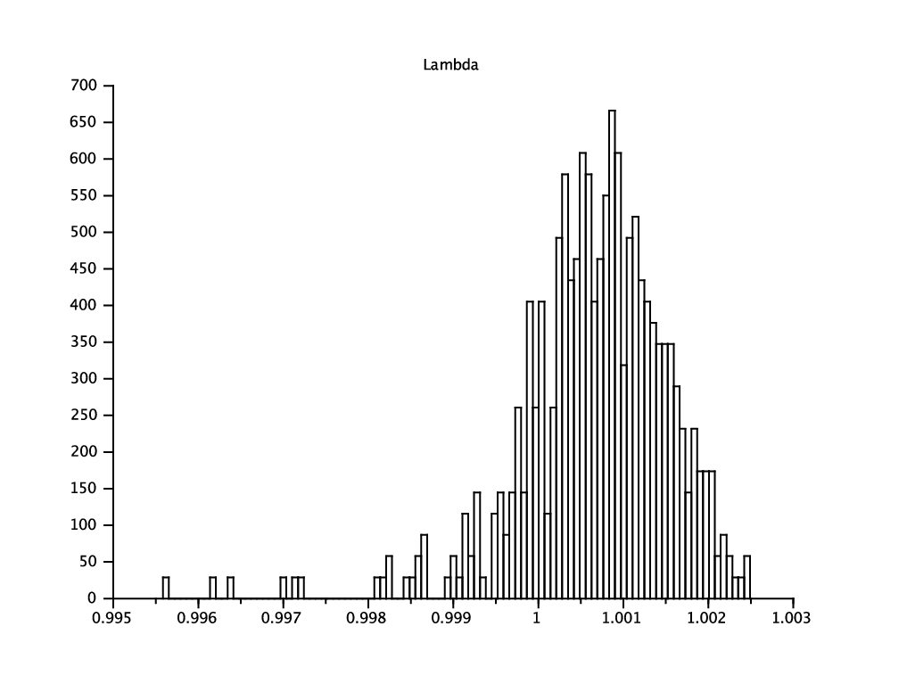
We next compare the variance of with the amount of randomness introduced in the function defined by (49). By construction,
with
which is an approximation of the relative variance of . We show on Figure 6 the histograms, for , of and of , for the initial guess parameter .
On this test-case, we compute that and , thus
On the other hand, , and , thus
We thus observe that the relative variance of the optimal parameters is roughly of the same order of magnitude as the relative variance introduced in the function to minimize. Given the amount of noise present in the system, our procedure robustly identifies the optimal parameters of the microscopic distribution.


Appendix A Computation of the derivatives of (49)
We introduce
and
where is defined by (48), and recast the function (49) as
where we have kept implicit the dependence with respect to . Computing the derivatives of therefore amounts to computing those of and .
A tedious but straightforward computation leads to the following expressions:
whereas
Acknowledgements. We thank Tony Lelièvre for giving us the opportunity to work on this problem during the CEMRACS 2013 (http://smai.emath.fr/cemracs/cemracs13/), and Nicolas Champagnat, Tony Lelièvre and Anthony Nouy for the organization of this event. We are grateful to Samir Békri, Daniel Coelho, Claude Le Bris, Tony Lelièvre and Benjamin Rotenberg for enlightening discussions. The work of FL and WM is partially supported by ONR under Grant N00014-12-1-0383. WM gratefully acknowledges the support from Labex MMCD (Multi-Scale Modelling & Experimentation of Materials for Sustainable Construction) under contract ANR-11-LABX-0022. WM, AO and MS acknowledge financial support from NEEDS Milieux Poreux.
References
- [1] A. Anantharaman, R. Costaouec, C. Le Bris, F. Legoll and F. Thomines, Introduction to numerical stochastic homogenization and the related computational challenges: some recent developments, W. Bao and Q. Du eds., Lecture Notes Series, Institute for Mathematical Sciences, National University of Singapore, volume 22, 197–272 (2011).
- [2] A. Bensoussan, J.-L. Lions and G. Papanicolaou, Asymptotic analysis for periodic structures, Studies in Mathematics and its Applications, vol. 5. North-Holland Publishing Co., Amsterdam-New York, 1978.
- [3] M. Biskup, Recent progress on the random conductance model, Probability Surveys, 8 (2011), 294–373.
- [4] X. Blanc, R. Costaouec, C. Le Bris and F. Legoll, Variance reduction in stochastic homogenization: the technique of antithetic variables, in Numerical Analysis and Multiscale Computations, B. Engquist, O. Runborg and R. Tsai eds., Lect. Notes Comput. Sci. Eng., vol. 82, Springer, 47-70 (2012).
- [5] X. Blanc, R. Costaouec, C. Le Bris and F. Legoll, Variance reduction in stochastic homogenization using antithetic variables, Markov Processes and Related Fields, 18(1) (2012), 31–66 (preliminary version available at http://cermics.enpc.fr/legoll/hdr/FL24.pdf).
- [6] A. Bourgeat and A. Piatnitski, Approximation of effective coefficients in stochastic homogenization, Ann I. H. Poincaré - PR, 40(2) (2004), 153–165.
- [7] D. Cioranescu and P. Donato, An introduction to homogenization, Oxford Lecture Series in Mathematics and its Applications, vol. 17. Oxford University Press, New York, 1999.
- [8] R. Costaouec, C. Le Bris and F. Legoll, Variance reduction in stochastic homogenization: proof of concept, using antithetic variables, Boletin Soc. Esp. Mat. Apl., 50 (2010), 9–27.
- [9] B. Engquist and P. E. Souganidis, Asymptotic and numerical homogenization, Acta Numerica, 17 (2008), 147–190.
- [10] I. Fatt, The network model of porous media, Trans. AIME, 207 (1956), 144–181.
- [11] A. Gloria, S. Neukamm and F. Otto, An optimal quantitative two-scale expansion in stochastic homogenization of discrete elliptic equations, Math. Modelling Numer. Analysis, in press, http://dx.doi.org/10.1051/m2an/2013110.
- [12] V. V. Jikov, S. M. Kozlov, and O. A. Oleinik, Homogenization of differential operators and integral functionals, Springer-Verlag, 1994.
- [13] R. Künnemann, The diffusion limit for reversible jump processes on with ergodic random bond conductivities, Comm. Math. Phys., 90(1) (1983), 27–68.
- [14] S. M. Kozlov, Averaging of difference schemes, Math. USSR Sbornik, 57(2) (1987), 351–369.
- [15] F. Legoll and W. Minvielle, Variance reduction using antithetic variables for a nonlinear convex stochastic homogenization problem, Discrete and Continuous Dynamical Systems - Series S, in press, arxiv preprint 1302.0038.
- [16] F. Legoll, W. Minvielle, A. Obliger and M. Simon, in preparation.