Fine-Grained Visual Categorization via
Multi-stage Metric Learning
Abstract
Fine-grained visual categorization (FGVC) is to categorize objects into subordinate classes instead of basic classes. One major challenge in FGVC is the co-occurrence of two issues: 1) many subordinate classes are highly correlated and are difficult to distinguish, and 2) there exists the large intra-class variation (e.g., due to object pose). This paper proposes to explicitly address the above two issues via distance metric learning (DML). DML addresses the first issue by learning an embedding so that data points from the same class will be pulled together while those from different classes should be pushed apart from each other; and it addresses the second issue by allowing the flexibility that only a portion of the neighbors (not all data points) from the same class need to be pulled together. However, feature representation of an image is often high dimensional, and DML is known to have difficulty in dealing with high dimensional feature vectors since it would require for storage and for optimization. To this end, we proposed a multi-stage metric learning framework that divides the large-scale high dimensional learning problem to a series of simple subproblems, achieving computational complexity. The empirical study with FVGC benchmark datasets verifies that our method is both effective and efficient compared to the state-of-the-art FGVC approaches.
1 Introduction
Fine-grained visual categorization (FGVC) aims to distinguish objects in subordinate classes. For example, dog images are classified into different breeds of dogs, such as “Chihuahua”, “Pug”, “Samoyed” and so on [17, 24]. One challenge of FGVC is that it has to handle the co-occurrence of two somewhat contradictory requirements: 1) it needs to distinguish

many similar classes (e.g., the dog breeds that only have subtle differences), and 2) it needs to deal with the large intra-class variation (e.g., caused by different poses, examples, etc.).
The popular pipeline for FVGC consists of two steps, feature extraction step and classification step. The feature extraction step, which sometimes combines with segmentation [1, 7, 24], part localization [2, 35] or both [6], is to extract image level representations, and popular choices include LLC features [1], Fisher vectors [14], etc. A recent development is to train the convolutional neural network (CNN) [18] on a large-scale image dataset (e.g., ImageNet [26]) and then use the trained model to extract features [12]. The so-called deep learning features have demonstrated the state-of-the-art performance on FGVC datasets [12]. Note that there has been some difficulties in training CNN directly on FGVC datasets because the existing FGVC benchmarks are often too small [12] (only several tens of thousands of training images or less). In this paper, we simply take the state-of-the-art deep learning features without any other operators (e.g., segmentation) and focus on studying better classification approach to address the aforementioned two co-occurring requirements in FGVC.
For the classification step, many existing FGVC methods directly learn a single classifier for each fine-grained class using the one-vs-all strategy [1, 2, 7, 35]. Apparently, this strategy does not scale well to the number of fine-grained classes while the number of subordinate classes in FGVC could be very large (e.g., 200 classes in birds11 dataset). Additionally, such one-vs-all scheme is only to address the first issue in the two issues, namely, it makes efforts to separate different classes without modeling intra-class variation. In this paper, we proposes a distance metric learning (DML) approach, aiming to explicitly handle the two co-occurring requirements with a single metric. Fig. 1 illustrates how DML works for FGVC. It learns a distance metric that pulls neighboring data points of the same class close to each other and pushes data points from different classes far apart. By varying the neighborhood size when learning the metric, it is able to effectively handle the tradeoff between the inter-class and intra-class variation. With a learned metric, a -nearest neighbor classifier will be applied to find the class assignment for a test image.
Although numerous algorithms have been developed for DML [8, 11, 32, 33], most of them are limited to low dimensional data (i.e. no more than a few hundred dimensions) while the dimensionality of image data representation is usually higher than [1]. A straightforward approach toward high dimensional DML is to reduce the dimensionality of data by using the methods such as principle component analysis (PCA) [32] and random projection [29]. The main problem with most dimensionality reduction methods is that they are unable to take into account the supervised information, and as a result, the subspaces identified by the dimensionality reduction methods are usually suboptimal.
There are three challenges in learning a metric directly from the original high dimensional space:
- •
Large number of constraints: A large number of training constraints are usually required to avoid the overfitting of high dimensional DML. The total number of triplet constraints could be up to where is the number of examples.
- •
Computational challenge: DML has to learn a matrix of size , where is the dimensionality of data and in our study. The number of variables leads to two computational challenges in finding the optimal metric. First, it results in a slower convergence rate in solving the related optimization problem [25]. Second, to ensure the learned metric to be positive semi-definitive (PSD), most DML algorithms require, at every iteration of optimization, projecting the intermediate solution onto a PSD cone, an expensive operation with complexity of (at least ).
- •
Storage limitation: It can be expensive to simply save number of variables in memory. For example, in our study, it would take more than 130 GB to store the completed metric in memory, which adds more complexity to the already difficult optimization problem.
In this work, we propose a multi-stage metric learning framework for high dimensional DML that explicitly addresses these challenges. First, to deal with a large number of constraints used by high dimensional DML, we divide the original optimization problem into multiple stages. At each stage, only a small subset of constraints that are difficult to be classified by the currently learned metric will be adaptively sampled and used to improve the learned metric. By setting the regularizer appropriately, we can prove that the final solution is optimized over all appeared constraints. Second, to handle the computational challenge in each subproblem, we extend the theory of dual random projection [36], which was originally developed for linear classification problems, to DML. The proposed method enjoys the efficiency of random projection, and on the other hand learns a distance metric of size . This is in contrast to most dimensionality reduction methods that learn a metric in a reduced space. Finally, to handle the storage problem, we propose to maintain a low rank copy of the learned metric by a randomized algorithm for low rank matrix approximation. It not only accelerates the whole learning process but also regularizes the learned metric to avoid overfitting. Extensive comparisons on benchmark FGVC datasets verify the effectiveness and efficiency of the proposed method.
2 Related Work
Many algorithms have been developed for DML [11, 32, 33] and a detailed review can be found in two survey papers [19, 34]. Some of them are based on pairwise constraints [11, 33], while others focus on optimizing triplet constraints [8, 32]. In this paper, we adopt triplet constraints, which exactly serve our purpose for addressing the second issue of FGVC. Although numerous studies were devoted to DML, few examined the challenges of high dimensional DML. A common approach for high dimensional DML is to project data into a low dimensional space, and learn a metric in the space of reduced dimension, which often leads to a suboptimal performance. An alternative approach is to assume to be of low rank by writing as [10, 32], where is a tall rectangle matrix and the rank of is fixed in advance of applying DML methods. Instead of learning , these approaches directly learn from data. The main shortcoming of this approach is that it has to solve a non-convex optimization problem, making it computationally less attractive. Several recent studies [20, 25] address high dimensional DML by assuming to be sparse. Although resolving the storage problem, they still suffer from high cost in optimizing variables.
3 Multi-stage Metric Learning
The proposed DML algorithm focuses on triplet constraints so as to pull the small portion of nearest examples from the same class together [32]. Let be a collection of training images, where and is the class assignment of . Given a distance metric , the distance between two data points and is measured by
Let be a set of triplet constraints derived from the training examples in . Since in each constraint , and share the same class assignment which is different from that of , we expect . As a result, the optimal distance metric is learned by solving the following optimization problem
| (1) |
where includes all real symmetric matrices and is a loss function that penalizes the objective function when is not significantly larger than . In this study, we choose the smoothed hinge loss [28] that appears to be more effective for optimization than the hinge loss while keeping the benefit of large margin
One main computational challenge of DML comes from the PSD constraint in (1). We address this challenge by following the one projection paradigm [8] that first learns a metric without the PSD constraint and then projects to the PSD cone at the very end of the learning process. Hence, in this study, we will focus on the following optimization problem for FGVC
| (3) |
where is introduced as a matrix representation for each triplet constraint, and represents the dot product between two matrices.
We will discuss the strategies to address the three challenges of high dimensional DML, and summarize the framework of high dimensional DML for FGVC at the end of this section.
3.1 Constraints Challenge: Multi-stage Division
In order to reliably determine the distance metric in a high dimensional space, a large number of training examples are needed to avoid the overfitting problem. Since the number of triplet constraints can be , the number of summation terms in (3) can be extremely large, making it difficult to effectively solve the optimization problem in (3). Although learning with active set may help reduce the number of constraints [32], the number of active constraints can still be very large since many images in FGVC from different categories are visually similar, leading to many mistakes. To address this challenge, we divide the learning process into multiple stages. At the -th stage, let be the distance metric learned from the last stage. We sample a subset of active triplet constraints that are difficult to be classified by (i.e., incur large hinge loss)11 1 The strategy of finding hard constraints at each stage is also applied by cutting plane methods [21] and active learning [27].. Given and the sampled triplet constraints , we update the distance metric by solving the following optimization problem
| (4) |
Although only a small size of constraints is used to improve the metric at each stage, we have
Theorem 1.
The metric learned by solving the problem (4) also optimizes the following objective function
Proof.
Consider the objective function for the first stages
| (5) |
It is obvious that is strongly convex, so we have (Chapter 9, [4])
for some between and .
Since , the solution obtained from the first stages, approximately optimizes and is -strongly convex, then
| (6) |
Remark
This theorem demonstrates that the metric learned from the last stage is optimized over constraints from all stages. Therefore, the original problem could be divided into several subproblems and each of them has an affordable number of active constraints. Fig. 2 summaries the framework of the multi-stage learning procedure.

3.2 Computational Challenge: Dual Random Projection
Now we try to solve the high dimensional subproblem by dual random projection technique. To simplify the analysis, we investigate the subproblem at the first stage and the following stages could be analyzed in the same way. By introducing the convex conjugate for in (4), the dual problem of DML is
| (7) |
where is the dual variable for and is a matrix defined as . by setting the gradient with respect to to zero. Let be two Gaussian random matrices, where is the number of random projections () and . For each triplet constraint, we project its representation into the low dimensional space using the random matrices, i.e. . By using double random projections, which is different from the single random projection in [36], we have
Lemma 1.
, the double random projections preserve the pairwise similarity between them:
The proof is straightforward. According to the lemma, the dual variables in (7) can be estimated in the low dimensional space as
| (8) |
where . Then, by the definition of convex conjugate, each dual variable in (8) can be further estimated by , where is the metric learned in the reduced space. Generally, is learned by solving the following optimization problem
| (9) |
Since the size of is significantly smaller than that of , (9) can be solved much more efficiently than (4). In our implementation, a simple stochastic gradient descent (SGD) method is developed to efficiently solve the optimization problem in (9). Given , the final distance metric in the original space is estimated as
| (10) |
3.3 Storage Challenge: Low Rank Approximation
Although (10) allows us to recover the distance metric in original dimensional space from the dual variables , it is expensive, if not impossible, to save in memory since is very large in FGVC [1]. To address this challenge, instead of saving , we propose to save the low rank approximation of . More specifically, let be the first eigenvalues of , and let be the corresponding eigenvectors. We approximate by a low rank matrix . Different from existing DML methods that directly optimize [31], we obtain first and then decompose it to avoid suboptimal solution. Unlike that requires storage space, it only takes space to save and could be an arbitrary value. In addition, the low rank metric accelerates the sampling step by reducing the cost of computing distance from to . Low rank is also a popular regularizer to avoid overfitting when learning high dimensional metric [20]. However, the key issue is how to efficiently compute the eigenvectors and eigenvalues of at each stage. This is particularly challenging in our case as in (10) even can not be computed explicitly due to its large size.
To address this problem, first we investigate the structure of the recovering step for the -th stage as in (10)
Therefore, we can express the summation as matrix multiplications. In particular, for each triplet , we denote its dual variable by and set the corresponding entries in a sparse matrix as
| (11) |
It is easy to verify that can be written as
| (12) |
Second, we exploit the randomized theory [15] to efficiently compute the eigen-decomposition of . More specifically, let () be an Gaussian random matrix. According to [15], with an overwhelming probability, most of the top eigenvectors of lie in the subspace spanned by the column vectors in provided , where is a constant independent from . The limitation of the method is that it requires the appearance of the matrix for computing while keeping the whole matrix is unaffordable here. Fortunately, by replacing with according to (12), we can approximate the top eigenvectors of by those of that is of size and can be computed efficiently since is a sparse matrix. The overall computational cost of the proposed algorithm for low rank approximation is only , which is linear in . Note that the sparse matrix is cumulated over all stages.
Alg. 1 summarizes the key steps of the proposed approach for low rank approximation, where and stand for QR and eigen decomposition of a matrix. Note that the distributed computing is particularly effective for the realization of the algorithm because the matrix multiplications can be accomplished in parallel, which is helpful when is also large.
Alg. 2 shows the whole picture of the proposed method.
4 Experiments
DeCAF features [12] are extracted as the image representations in the experiments. Although it is from the activation of a deep convolutional network, which is trained on ImageNet [18], it outperforms conventional visual features on many general tasks [12]. We concatenate features from the last three fully connected layers (i.e., DeCAF5+6+7) and the dimension of resulting features is .
We apply the proposed algorithm to learn a distance metric and use the learned metric together with a smoothed -nearest neighbor classifier, a variant of -NN, to predict the class assignments for test examples. Different from conventional -NN, it first obtains reference centers for each class by clustering training images in each class into clusters. Then, it computes the query’s distance to each class as the soft min of the distances between the test image and corresponding reference centers, and assigns the test image to the class with the shortest distance. It is more efficient when predicting, especially for large-scale training set, and the performance is similar to that of conventional one. We refer to the classification approach based on the metric learned by the proposed algorithm and the smoothed -NN as MsML, and the smoothed -NN with Euclidean distance in the original space as Euclid. Although the size of the covariance matrix is very large (), its rank is low due to the small number of training examples, and thus PCA can be computed explicitly. The state-of-the-art DML algorithm, i.e. LMNN [32] with PCA as preprocess, is also included in comparison. The one-vs-all strategy, based on the implementation of LIBLINEAR [13], is used as a baseline for FGVC, with the regularization parameter varied in the range . We refer to it as LSVM. We also include the state-of-the-art results for FGVC in our evaluation. All the parameters used by MsML are set empirically, with the number of random projections and the number of random combinations . PCA is applied for LMNN to reduce the dimensionality to before the metric is learned. LMNN is implemented by the code from the original authors and the recommended parameters are used 22 2 We did vary the parameter slightly from the recommended values and did not find any noticeable change in the classification accuracy.. To ensure that the baseline method fully exploits the training data, we set the maximum number of iterations for LMNN as . These parameter values are used throughout all the experiments. All training/test splits are provided by datasets. Mean accuracy, a standard evaluation metric for FGVC, is used to evaluate the classification performance. All experiments are run on a single machine with GHz cores and GB memory.
4.1 Oxford Cats&Dogs
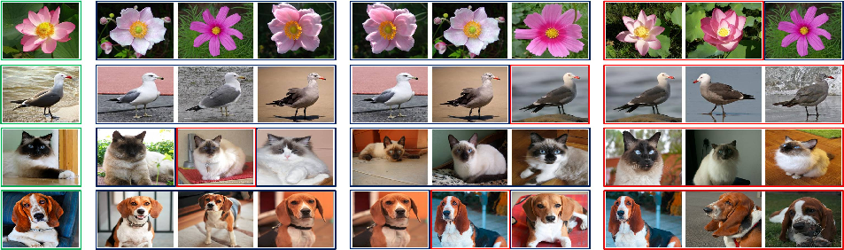
cats&dogs contains images from cat and dog species [24]. There are about 100 images per class for training and the rest are for test. Table 1 summaries the results. First, we observe that MsML is more accurate than the baseline LSVM. This is not surprising because the distance metric is learned from the training examples of all class assignments. This is in contrast to the one-vs-all approach used in LSVM that the classification function for a class is learned only by the examples with the class assignment of . Second, our method performs significantly better than the baseline DML method, indicating that the unsupervised dimension reduction method PCA may result in suboptimal solutions for DML. Fig. 3 compares the images that are most similar to the query images using the metric learned by the proposed algorithm (Column 8-10) to those based on the metric learned by LMNN (Column 5-7) and Euclid (Column 2-4). We observe that more images from the same class as the query are found by the metric learned by MsML than LMNN. For example, MsML is able to capture the difference between two cat species (longhair v.s. shorthair) while LMNN returns the very similar images with wrong class assignments. Third, MsML has overwhelming performance compared to all state-of-the-art FGVC approaches. Although the method [24] using ground truth head bounding box and segmentation achieves , MsML is better than it with only image information, which shows the advantage of the proposed method. Finally, it takes less than second to extract DeCAF features per image based on a implementation while a simple segmentation operator costs more than 2.5 seconds as reported in the study [1], making the proposed method for FGVC more appealing.
| Methods | Mean Accuracy () |
|---|---|
| Image only [24] | 39.64 |
| Det+Seg [1] | 54.30 |
| Image+Head+Body# [24] | 59.21 |
| Euclid | 72.60 |
| LSVM | 77.63 |
| LMNN | 76.24 |
| MsML | 80.45 |
| MsML+ | 81.18 |
To evaluate the performance of MsML for extremely high dimensional features, we concatenate conventional features by using the pipeline for visual feature extraction that is outlined in [1]. Specifically, we extract HOG [9] features at 4 different scales and encode them to dimensional feature dictionary by the LLC method [31]. A max pooling strategy is then used to aggregate local features into a single vector representation. Finally, features are extracted from each image and the total dimension is up to . MsML with the combined features is denoted as MsML+ and it further improves the performance by about as in Table 1. Note that the time of extracting these high dimensional conventional features is only second per image, which is still much cheaper than any segmentation or localization operator.
4.2 Oxford 102 Flowers
102flowers is the Oxford flowers dataset for flower species [23], which consists of 8189 images from 102 classes. Each class has 20 images for training and rest for test. Table 2 shows the results from different methods. We have the similar conclusion for the baseline methods. That is, MsML outperforms LSVM and LMNN significantly. Although LSVM already performs very well, MsML further improves the accuracy. Additionally, it is observed that even the performances of state-of-the-art methods with segmentation operators are much worse than that of MsML. Note that GT [23] uses hand annotated segmentations followed by multiple kernel SVM, while MsML outperforms it about without any supervised information, which confirms the effectiveness of the proposed method.
| Methods | Mean Accuracy () |
|---|---|
| Combined CoHoG [16] | 74.80 |
| Combined Features [22] | 76.30 |
| BiCoS-MT [5] | 80.00 |
| Det+Seg [1] | 80.66 |
| TriCoS [7] | 85.20 |
| GT# [23] | 85.60 |
| Euclid | 76.21 |
| LSVM | 87.14 |
| LMNN | 81.93 |
| MsML | 88.39 |
| MsML+ | 89.45 |
Fig. 4.2 illustrates the changing trend of test mean accuracy as the number of stages increases. We observe that MsML converges very fast, which verifies that multi-stage division is essential to the proposed framework.


4.3 Birds-2011
birds11 is the Caltech-USCD-200-2011 birds dataset for bird species [30]. There are 200 classes with images and each class has roughly 30 images for training. We use the version with ground truth bounding box. Table 3 compares the proposed method to the state-of-the-art baselines. First, it is obvious that the performance of MsML is significantly better than all baseline methods as the observation above. Second, although Symb [6] combines segmentation and localization, MsML outperforms it by without any time consuming operator. Third, Symb* and Ali* mirror the training images to improve their performances, while MsML is even better than them without this trick. Finally, MsML outperforms the method combining DeCAF features and DPD models [37], which is due to the fact that most of studies for FGVC ignore choosing the appropriate base classifier and simply adopt linear SVM with the one-vs-all strategy. For comparison, we also report the result mirroring training images which is denoted as MsML+*. It provides another improvement over MsML+ as shown in Table 3.
To illustrate the capacity of MsML in exploring the correlation among classes, which makes it more effective than a simple one-vs-all classifier for FGVC, we conduct one additional experiment. We randomly select 50 classes from birds11 as the target classes and use the test images from the target classes for evaluation. When learning the metric, besides the training images from target classes, we sample classes from unselected ones as the auxiliary classes, and use training images from the auxiliary classes as additional training examples for DML. Fig. 4.2 compares the performance of LSVM and MsML with the increasing number of auxiliary classes. It is not surprising to observe that the performance of LSVM decreases a little since it is unable to explore the supervision information in the auxiliary classes to improve the classification accuracy of target classes and more auxiliary classes just intensify the class imbalance problem. In contrast, the performance of MsML improves significantly with increasing auxiliary classes, indicating that MsML is capable of effectively exploring the training data from the auxiliary classes and therefore is particularly suitable for FGVC.
4.4 Stanford Dogs
4.5 Comparison of Efficiency
In this section, we compare the training time of the proposed algorithm for high dimensional DML to that of LSVM and LMNN. MsML is implemented by Julia, which is a little slower than C33 3 Detailed comparison can be found in http://julialang.org, while LSVM uses the LIBLINEAR package, the state-of-the-art algorithm for solving linear SVM implemented mostly in C. The core part of LMNN is also implemented in C. The time for feature extraction is not included here because it is shared by all the methods in comparison. The running time for MsML includes all operational cost (i.e., the cost for sampling triplet constraints, computing random projections and low rank approximation).
| Methods | cats&dogs | 102flowers | birds11 | S-dogs |
|---|---|---|---|---|
| LSVM | 196.2 | 309.8 | 1,417.0 | 1,724.8 |
| LMNN | 832.6 | 702.7 | 1,178.2 | 1,643.6 |
| MsML | 164.9 | 174.4 | 413.1 | 686.3 |
| MsML+ | 337.2 | 383.7 | 791.3 | 1,229.7 |
Table 5 summarizes the results of the comparison. First, it takes MsML about of the time to complete the computation compared to LMNN. This is because MsML employs a stochastic optimization method to find the optimal distance metric while LMNN is a batch learning method. Second, we observe that the proposed method is significantly more efficient than LSVM on most of datasets. The high computational cost of LSVM mostly comes from two aspects. First, LSVM has to train one classification model for each class, and becomes significantly slower when the number of classes is large. Second, the fact that images from different classes are visually similar makes it computationally difficult to find the optimal linear classifier that can separate images of one class from images from the other classes. In contrast, the training time of MsML is independently from the number of classes, making it more appropriate for FGVC. Finally, the running time of MsML+ with features only doubles that of MsML, which verifies that the proposed method is linear in dimensionality ().
5 Conclusion
In this paper, we propose a multi-stage metric learning framework for high dimensional FGVC problem, which addresses the challenges arising from high dimensional DML. More specifically, it divides the original problem into multiple stages to handle the challenge arising from too many triplet constraints, extends the theory of dual random projection to address the computational challenge for high dimensional data, and develops a randomized low rank matrix approximation algorithm for the storage challenge. The empirical study shows that the proposed method with general purpose features yields the performance that is significantly better than the state-of-the-art approaches for FGVC. In the future, we plan to combine the proposed DML algorithm with segmentation and localization to further improve the performance of FGVC. Additionally, since the proposed method is a general DML approach, we will try to apply it for other applications with high dimensional features.
Acknowledgments
Qi Qian and Rong Jin are supported in part by ARO (W911NF-11-1-0383), NSF (IIS-1251031) and ONR (N000141410631).
References
- [1] A. Angelova and S. Zhu. Efficient object detection and segmentation for fine-grained recognition. In CVPR, 2013.
- [2] T. Berg and P. N. Belhumeur. Poof: Part-based one-vs-one features for fine-grained categorization, face verification, and attribute estimation. In CVPR, 2013.
- [3] T. Berg and P. N. Belhumeur. POOF: part-based one-vs.-one features for fine-grained categorization, face verification, and attribute estimation. In CVPR, pages 955–962, 2013.
- [4] S. Boyd and L. Vandenberghe. Convex optimization. Cambridge university press, 2009.
- [5] Y. Chai, V. S. Lempitsky, and A. Zisserman. Bicos: A bi-level co-segmentation method for image classification. In ICCV, pages 2579–2586, 2011.
- [6] Y. Chai, V. S. Lempitsky, and A. Zisserman. Symbiotic segmentation and part localization for fine-grained categorization. In ICCV, pages 321–328, 2013.
- [7] Y. Chai, E. Rahtu, V. S. Lempitsky, L. J. V. Gool, and A. Zisserman. Tricos: A tri-level class-discriminative co-segmentation method for image classification. In ECCV, pages 794–807, 2012.
- [8] G. Chechik, V. Sharma, U. Shalit, and S. Bengio. Large scale online learning of image similarity through ranking. JMLR, 11:1109–1135, 2010.
- [9] N. Dalal and B. Triggs. Histograms of oriented gradients for human detection. In CVPR, pages 886–893, 2005.
- [10] J. V. Davis and I. S. Dhillon. Structured metric learning for high dimensional problems. In KDD, pages 195–203, 2008.
- [11] J. V. Davis, B. Kulis, P. Jain, S. Sra, and I. S. Dhillon. Information-theoretic metric learning. In ICML, pages 209–216, 2007.
- [12] J. Donahue, Y. Jia, O. Vinyals, J. Hoffman, N. Zhang, E. Tzeng, and T. Darrell. Decaf: A deep convolutional activation feature for generic visual recognition. In ICML, pages 647–655, 2014.
- [13] R.-E. Fan, K.-W. Chang, C.-J. Hsieh, X.-R. Wang, and C.-J. Lin. LIBLINEAR: A library for large linear classification. JMLR, 9:1871–1874, 2008.
- [14] E. Gavves, B. Fernando, C. G. M. Snoek, A. W. M. Smeulders, and T. Tuytelaars. Fine-grained categorization by alignments. In ICCV, pages 1713–1720, 2013.
- [15] N. Halko, P.-G. Martinsson, and J. A. Tropp. Finding structure with randomness: Probabilistic algorithms for constructing approximate matrix decompositions. ArXiv e-prints, Sept. 2009.
- [16] S. Ito and S. Kubota. Object classification using heterogeneous co-occurrence features. In ECCV, pages 209–222, 2010.
- [17] A. Khosla, N. Jayadevaprakash, B. Yao, and F.-f. Li. Novel dataset for fine-grained image categorization. In First Workshop on Fine-Grained Visual Categorization, CVPR, 2011.
- [18] A. Krizhevsky, I. Sutskever, and G. E. Hinton. Imagenet classification with deep convolutional neural networks. In NIPS, pages 1106–1114, 2012.
- [19] B. Kulis. Metric learning: A survey. Foundations and Trends in Machine Learning, 5(4):287–364, 2013.
- [20] D. K. H. Lim, B. McFee, and G. Lanckriet. Robust structural metric learning. In ICML, 2013.
- [21] Y. Nesterov. Introductory lectures on convex optimization, volume 87. Springer Science & Business Media, 2004.
- [22] M.-E. Nilsback. An Automatic Visual Flora – Segmentation and Classification of Flowers Images. PhD thesis, University of Oxford, 2009.
- [23] M.-E. Nilsback and A. Zisserman. Automated flower classification over a large number of classes. In ICVGIP, pages 722–729, 2008.
- [24] O. M. Parkhi, A. Vedaldi, A. Zisserman, and C. V. Jawahar. Cats and dogs. In CVPR, pages 3498–3505, 2012.
- [25] G.-J. Qi, J. Tang, Z.-J. Zha, T.-S. Chua, and H.-J. Zhang. An efficient sparse metric learning in high-dimensional space via l-penalized log-determinant regularization. In ICML, page 106, 2009.
- [26] O. Russakovsky, J. Deng, H. Su, J. Krause, S. Satheesh, S. Ma, Z. Huang, A. Karpathy, A. Khosla, M. Bernstein, A. C. Berg, and L. Fei-Fei. ImageNet Large Scale Visual Recognition Challenge, 2014.
- [27] B. Settles. Active learning literature survey. University of Wisconsin, Madison, 52(55-66):11, 2010.
- [28] S. Shalev-Shwartz and T. Zhang. Stochastic dual coordinate ascent methods for regularized loss minimization. CoRR, abs/1209.1873, 2012.
- [29] G. Tsagkatakis and A. E. Savakis. Manifold modeling with learned distance in random projection space for face recognition. In ICPR, pages 653–656, 2010.
- [30] C. Wah, S. Branson, P. Welinder, P. Perona, and S. Belongie. The Caltech-UCSD Birds-200-2011 Dataset. Technical report, 2011.
- [31] J. Wang, J. Yang, K. Yu, F. Lv, T. S. Huang, and Y. Gong. Locality-constrained linear coding for image classification. In CVPR, pages 3360–3367, 2010.
- [32] K. Q. Weinberger and L. K. Saul. Distance metric learning for large margin nearest neighbor classification. JMLR, 10:207–244, 2009.
- [33] E. P. Xing, A. Y. Ng, M. I. Jordan, and S. J. Russell. Distance metric learning with application to clustering with side-information. In NIPS, pages 505–512, 2002.
- [34] L. Yang and R. Jin. Distance metric learning: a comprehensive survery. 2006.
- [35] S. Yang, L. Bo, J. Wang, and L. G. Shapiro. Unsupervised template learning for fine-grained object recognition. In NIPS, pages 3131–3139, 2012.
- [36] L. Zhang, M. Mahdavi, R. Jin, T.-B. Yang, and S. Zhu. Recovering optimal solution by dual random projection. In arXiv:1211.3046, 2013.
- [37] N. Zhang, R. Farrell, F. N. Iandola, and T. Darrell. Deformable part descriptors for fine-grained recognition and attribute prediction. In ICCV, pages 729–736, 2013.