Optimisation of Bell inequalities with invariant Tsirelson bound

M Epping Affiliation: Institut für Theoretische Physik III, Heinrich-Heine-Universität Düsseldorf, Universitätsstrasse 1, D-40225 Düsseldorf, Germany H Kampermann Affiliation: Institut für Theoretische Physik III, Heinrich-Heine-Universität Düsseldorf, Universitätsstrasse 1, D-40225 Düsseldorf, Germany D Bruß Email: epping@thphy.uni-duesseldorf.de Email: Affiliation: Institut für Theoretische Physik III, Heinrich-Heine-Universität Düsseldorf, Universitätsstrasse 1, D-40225 Düsseldorf, Germany

August 24, 2026

Abstract

We consider a subclass of bipartite CHSH-type Bell inequalities. We investigate operations, which leave their Tsirelson bound invariant, but change their classical bound. The optimal observables are unaffected except for a relative rotation of the two laboratories. We illustrate the utility of these operations by giving explicit examples: We prove that for a fixed quantum state and fixed measurement setup except for a relative rotation of the two laboratories, there is a Bell inequality that is maximally violated for this rotation, and we optimise some Bell inequalities with respect to the maximal violation. Finally we optimise the qutrit to qubit ratio of some dimension witnessing Bell inequalities.

1 Introduction

Originally, John S. Bell introduced what we now call Bell inequalities in order to show that the ideas of locality and realism are incompatible with statistical predictions of quantum theory [1]. Thus, the question whether a completion of quantum theory obeying these axioms exists, as proposed by Einstein, Podolski and Rosen [2], was brought to an experimentally testable level. Now, fifty years later, there is very strong experimental evidence that Bell inequalities can be violated by nature [3, 4, 5, 6, 7, 8, 9, 10], which implies that not all axioms in the derivation of Bell inequalities are followed by nature. Nevertheless Bell inequalities are not water under the bridge yet. This is amongst other reasons due to several interesting applications, like quantum key distribution, where the violation of Bell inequalities is a test for eavesdropping [11]. Here and in other applications, the amount of violation becomes important and a stronger violation of the inequality is usually beneficial (e.g. noise is less corruptive or the gap between classical and quantum performance increases).
In the present paper, we discuss two methods to modify Bell inequalities, which change the classical bound but leave the maximal value achievable in quantum theory unchanged. These methods can be used to optimise Bell inequalities with respect to the possible amount of violation. Various research on Bell inequalities with a large amount of violation has been carried out [12, 13, 14, 15], but literature on the specific problem investigated in this paper is less extensive [16, 17].
We specify the Bell inequalities under consideration in the following Section 2. Then we formulate the above-mentioned methods as a Corollary in Section 3 and give examples for their utility in Section 4. Section 5 concludes this paper.

2 A subclass of CHSH-type Bell inequalities

We consider bipartite full correlation Bell inequalities (CHSH type Bell inequalities [18, 19]) with $M_{i}$ measurement settings at the site of party $i$ . These settings are labelled $x_{i}=1,2,...,M_{i}$ . Such Bell inequalities can be written in the form

\sum_{x_{1},x_{2}=1}^{M_{1},M_{2}}g_{x_{1},x_{2}}E(x_{1},x_{2})\leq B,

(1)

where $E(x_{1},x_{2})$ is the expectation value for setting $x_{1}$ at Alice’s site and $x_{2}$ at Bob’s site and $g$ is a real $M_{1}\times M_{2}$ -matrix of coefficients. Measurement outcomes are required to be in the interval $[-1,1]$ . The dimension of the two subsystems is not fixed. The local hidden variable bound $B$ holds for all values achievable in local hidden variable theories, i.e.

\max_{a_{1},a_{2}}\sum_{x_{1},x_{2}=1}^{M_{1},M_{2}}g_{x_{1},x_{2}}a_{1}(x_{1})a_{2}(x_{2})\leq B.

(2)

$B$ can be calculated by performing this maximisation over all possible (deterministically) predefined measurement outcomes $a_{1}(x_{1})=\pm 1$ and $a_{2}(x_{2})=\pm 1$ . Due to the assumption of locality, $a_{1}$ ( $a_{2}$ ) does not depend on $x_{2}$ ( $x_{1}$ ). The use of unmeasured outcomes is motivated by the assumption of realism. See [20] for a more thorough analysis. For some $g$ , Inequality (2) can be violated within quantum theory.
Similarly, one can write down bounds for expectation values predicted by quantum theory [21]. The analogue of Ineq (1) reads

\sum_{x_{1},x_{2}=1}^{M_{1},M_{2}}g_{x_{1},x_{2}}E(x_{1},x_{2})\leq T,

(3)

where $T$ is a Tsirelson bound, which holds for all quantum states given by a density matrix $\rho$ and all observables $\mathcal{A}_{1}(x_{1})$ and $\mathcal{A}_{2}(x_{2})$ , i.e.

\max_{\mathcal{A}_{1},\mathcal{A}_{2},\rho}\sum_{x_{1},x_{2}=1}^{M_{1},M_{2}}g_{x_{1},x_{2}}\tr\left(\rho\mathcal{A}_{1}(x_{1})\otimes\mathcal{A}_{2}(x_{2})\right)\leq T.

(4)

Remember that we did not restrict the dimension of the Hilbert space. In [22] we showed that a quantum bound for Inequality (3) is given by

T(g)=||g||_{2}\sqrt{M_{1}M_{2}},

(5)

where $||g||_{2}$ is the largest singular value of $g$ . However, this bound $T$ is not always tight: It is not always possible to achieve equality in Inequality (4). Nevertheless it is tight for a subclass of Bell inequalities, which contains many well-known Bell inequalities. In this paper we will restrict ourselves to this class of Bell inequalities, for which $T$ in Eq. (5) is achievable for some states and observables. In this case the violation of the Bell inequality, which is the ratio of the quantum and the classical value, is

\nu=\frac{T}{B}.

(6)

According to a theorem by Tsirelson [23], there exist real vectors $\vec{v}_{1}$ , $\vec{v}_{2}$ , …, $\vec{v}_{M_{1}}$ and $\vec{w}_{1}$ , $\vec{w}_{2}$ , …, $\vec{w}_{M_{2}}$ , such that the quantum mechanical expectation value can be written as

E(x_{1},x_{2})=\vec{v}_{x_{1}}^{T}\vec{w}_{x_{2}}.

(7)

In the present context, it is usually more convenient to use these vectors instead of the observables. Let $g$ be a real $M_{1}\times M_{2}$ -matrix and $V$ , $S$ , $W$ be a singular value decomposition of $g$ , i.e. $g=VSW^{T}$ with diagonal $S$ and $V$ , $W$ being orthogonal. We denote the dimension of the space of the largest singular value $||g||_{2}$ as $d$ , i.e. this is the degeneracy of the largest singular value. The corresponding matrices of the truncated singular value decomposition associated with $||g||_{2}$ contain the first $d$ columns (the singular vectors) of $V$ and $W$ , respectively.

Theorem 1 (Tightness of $T$ [22]).

For any real $M_{1}\times M_{2}$ matrix $g$ , let $V^{d}$ , $||g||_{2}\mathds{1}^{d}$ , $W^{d}$ be a truncated singular value decomposition of $g$ associated with $||g||_{2}$ , where $d$ is the degeneracy of $||g||_{2}$ . The bound $T=||g||_{2}\sqrt{M_{1}M_{2}}$ can be reached with observables, which are linked via $E(i,j)=\vec{v}_{i}^{T}\vec{w}_{j}$ to $d^{\prime}\leq d$ -dimensional real vectors $\vec{v}_{i}$ and $\vec{w}_{j}$ given by

	$\displaystyle\hphantom{\mbox{and }{}}\vec{v}_{i}$	$\displaystyle=$	$\displaystyle\alpha^{T}V^{d}_{i,*}$		(8)
	$\displaystyle\mbox{and }\vec{w}_{j}$	$\displaystyle=$	$\displaystyle\sqrt{\frac{M_{2}}{M_{1}}}\alpha^{T}W^{d}_{j,*},$		(9)

if and only if there exists a $d\times d^{\prime}$ -matrix $\alpha$ , such that these vectors are normalised. Here $V^{d}_{i,*}$ and $W^{d}_{j,*}$ denote column vectors containing the elements of the $i$ -th row of $V^{d}$ and the $j$ -th row of $W^{d}$ , respectively.

There is a geometric interpretation of the norm conditions: The bound $T$ is tight for observables corresponding to $d^{\prime}$ -dimensional real vectors $\vec{v}_{i}$ and $\vec{w}_{j}$ if and only if the vectors $V_{i,*}^{d}$ and $\sqrt{\frac{M_{2}}{M_{1}}}W_{j,*}^{d}$ lie on the surface of an origin-centred ellipsoid with no more than $d^{\prime}$ finite semi-axes [22]. We call this object a $d^{\prime}$ -dimensional ellipsoid.

3 Modifying Bell inequalities inside this class

We aim at modifying Bell inequalities inside the class described in the previous section, i.e. those where the quantum bound given in Eq. (5) is tight. In particular, we are interested in operations that do not change the value of $T$ given in Eq. (5). However, in general these operations do change the classical bound of the Bell inequality, i.e. the modification’s effect on the quantum and the classical value are qualitatively and quantitatively different. This is in contrast to arbitrary modifications of the coefficients, where both values are simultaneously affected. We will exemplify later that such modifications can be a useful tool, e.g. for optimising Bell inequalities. The following corollary gives modifications with the properties we are seeking.

Corollary 1.

Let $g$ be a $M_{1}\times M_{2}$ real matrix with singular value decomposition $V$ , $S$ , $W$ , i.e. $g=VSW^{T}$ , such that $T(g)$ is achievable. The multiplicity of $||g||_{2}$ is denoted by $d$ , the length of the diagonal of $S$ is $s=\min(M_{1},M_{2})$ . The following modifications of $g$ lead to achievable bounds $T(g^{\prime})$ (primed symbols correspond to the modified coefficients $g^{\prime}$ ).

1.

”Twisting” of singular vectors:
For

$g^{\prime}=V\left(\begin{array}[]{cc}R_{1}&0\\ 0&R_{2}\end{array}\right)S\left(\begin{array}[]{cc}\mathds{1}^{d}&0\\ 0&R_{3}\end{array}\right)W^{T},$ (10)

where $R_{1}$ is a $d\times d$ orthogonal matrix commuting with $\alpha$ (see Eq. (8)) and $R_{2}$ and $R_{3}$ are orthogonal matrices of dimension $(M_{1}-d)$ and $(M_{2}-d)$ , respectively, $T(g^{\prime})=T(g)$ is achievable.

Modification of singular values:
For signs $\sigma_{1},...,\sigma_{d}=\pm 1$ and real numbers $\lambda_{1},\lambda_{d+1},\lambda_{d+2},...,\lambda_{s}$ fulfilling

|\lambda_{i}+S_{i,i}|<\left|\,||g||_{2}+\lambda_{1}\right|\mbox{ for all }i>d

(11)

the modified coefficients $g^{\prime}=VS^{\prime}W^{T}$ with

S^{\prime}=\mbox{diag}(\sigma_{1}(S_{1,1}+\lambda_{1}),...,\sigma_{d}(S_{d,d}+\lambda_{1}),S_{d+1,d+1}+\lambda_{d+1},...,S_{s,s}+\lambda_{s})

(12)

correspond to an inequality with achievable $T(g^{\prime})=\frac{||g||_{2}+\lambda_{1}}{||g||_{2}}T(g)$ .

Proof.

1.

$R_{1}$ can be considered as a rotation of the singular vectors, i.e. the singular values in $S$ are not affected. If $R_{1}$ and the $d\times d$ -matrix $\alpha$ commute, then

$||\alpha^{T}(R_{1}^{T}V_{i,*}^{d})||=||R_{1}^{T}\alpha^{T}V_{i,*}^{d}||=||\alpha^{T}V_{i,*}^{d}||,$ (13)

i.e. the conditions of Theorem 1 are not affected. $R_{2}$ and $R_{3}$ merely rotate the singular vectors outside the space associated with $||g||_{2}$ , which neither affects the tightness nor the value of the bound.
2.

The conditions for tightness according to Theorem 1 and the value of $T$ are not affected by modification of non-maximal singular values, as long as they do not become maximal. Adding the same value to all largest singular values is only a scaling of $T$ (as long as they remain maximal). A negative diagonal entry induces a sign change of the elements of the corresponding singular vector.

∎

Please note that the condition of (1) is fulfilled, if there exists a solution $\alpha\propto\mathds{1}$ .
We remark that (2) is a generalisation of the diagonal modification in [16]. There, $V=W$ and $g^{\prime}=g+\lambda\mathds{1}$ , which corresponds to $\lambda_{i}=\lambda$ . The condition of Eq. (11) on the $\lambda_{i}$ can be ignored, if one assures tightness according to Theorem 1. For example, depending on the particular form of $V$ and $W$ , the bound might be tight for different values of $d$ . In particular, $T$ is tight, if the new singular values are all equal. Furthermore (2) includes the special case, where $g^{\prime}=rg$ for any $r\in\mathds{R}$ .

4 Using these modifications as a method

In this section, the modifications described in Corollary 1 are applied to specific examples of coefficient matrices $g$ .

4.1 Maximally violated Bell inequality for relative rotation of laboratories

We start with the modification (1), i.e. the twisting of the singular vectors. First we note that $R_{1}$ is a relative rotation of the two parties in the sense, that the real vectors $\vec{v}_{x_{1}}$ , which define optimal observables for party one, are rotated by $R_{1}$ . For $d^{\prime}=3$ , one can interpret $\vec{v}_{x_{1}}$ as a Bloch-vector, i.e. $\mathcal{A}(x_{1})=\vec{v}_{x_{1}}^{T}\vec{\sigma}$ , where $\vec{\sigma}$ denotes the vector containing the three Pauli matrices. In this way we see that the rotation $R_{1}$ corresponds to a relative rotation of the two laboratories in the usual sense.
This motivates us to prove the following statement.

Example 1.

For every relative rotation between the laboratories of party one and party two, there exists a Bell inequality that is maximally violated for exactly this rotation. We require that the experimental setup is fixed up to the relative rotation, i.e. the measurement directions in the local coordinate systems and the shared state (e.g. $|\phi^{+}\rangle=\frac{1}{\sqrt{2}}(|00\rangle+|11\rangle)$ ) do not depend on the rotation angle. Consider the Bell inequalities given via the coefficient matrix

g=\left(\begin{array}[]{ccc}\frac{1}{2}&\frac{1}{2}&0\\ -\frac{1}{2}&\frac{1}{2}&0\\ 0&0&\frac{1}{\sqrt{2}}\\ \frac{1}{\sqrt{2}}&0&0\\ 0&\frac{1}{\sqrt{2}}&0\\ 0&0&\frac{1}{\sqrt{2}}\\ \end{array}\right)R(\Phi,\Theta,\Psi),

(14)

where

	$\displaystyle R(\Phi,\Theta,\Psi)$	$\displaystyle=$	$\displaystyle\phantom{{}\times{}}\left(\begin{array}[]{ccc}1&0&0\\ 0&\cos(\Phi)&\sin(\Phi)\\ 0&-\sin(\Phi)&\cos(\Phi)\\ \end{array}\right)\times$
			$\displaystyle\times\left(\begin{array}[]{ccc}\cos(\Theta)&0&-\sin(\Theta)\\ 0&1&0\\ \sin(\Theta)&0&\cos(\Theta)\\ \end{array}\right)\left(\begin{array}[]{ccc}\cos(\Psi)&\sin(\Psi)&0\\ -\sin(\Psi)&\cos(\Psi)&0\\ 0&0&1\\ \end{array}\right)$

is a general rotation given by the roll-pitch-yaw angle. From Eq (14) one can read the truncated singular value decomposition associated with the threefold ( $d=3$ ) degenerate maximal singular value $1$ : i.e the first factor is $V^{d}$ , $S^{d}=\mathds{1}$ and $W^{T}=R(\Phi,\Theta,\Psi)$ . From this we already know that $T(g)=\sqrt{M_{1}M_{2}}=3\sqrt{2}$ for all angles. This bound is achievable, because $\alpha=\sqrt{2}\mathds{1}^{3}$ is a solution (see Theorem 1). The vectors $V_{1,*}^{d}$ , $V_{2,*}^{d}$ , $V_{4,*}^{d}$ , $V_{5,*}^{d}$ force the rank of $\alpha$ to be at least two (two or more semi-axes of the corresponding ellipsoid are finite). Therefore, the inequality associated with $g$ is really a Bell inequality, i.e. it can be violated. The bound is achieved for the state $|\phi^{+}\rangle=\frac{1}{\sqrt{2}}(|00\rangle+|11\rangle)$ with observables

	$\displaystyle\mathcal{A}(x_{1})$	$\displaystyle=$	$\displaystyle\vec{v}_{x_{1}}^{T}\vec{\sigma},$		(26)
	$\displaystyle\mathcal{A}(x_{2})$	$\displaystyle=$	$\displaystyle(\vec{w}_{x_{2}}^{T}\vec{\sigma})^{T}.$		(27)

Because

\vec{w}_{j}=\sqrt{\frac{M_{2}}{M_{1}}}\alpha^{T}W_{j,*}^{d}=R(\Phi,\Theta,\Psi)_{j,*},

(28)

i.e. the measurement directions of party two are given by the columns of $R^{T}(\Phi,\Theta,\Psi)$ , this Bell inequality is maximally violated for a relative rotation of the laboratories given by the roll-pitch-yaw angle (see Figure 1 (a)). The violation $\frac{T}{B}$ of the inequality given by the coefficients in Eq. (14) depends on the angles (see Figure 1 (b,c,d)).

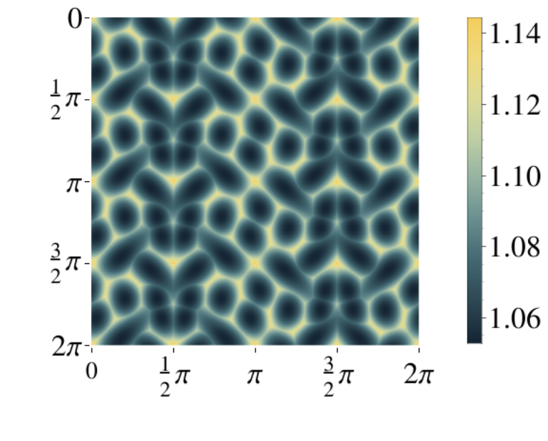
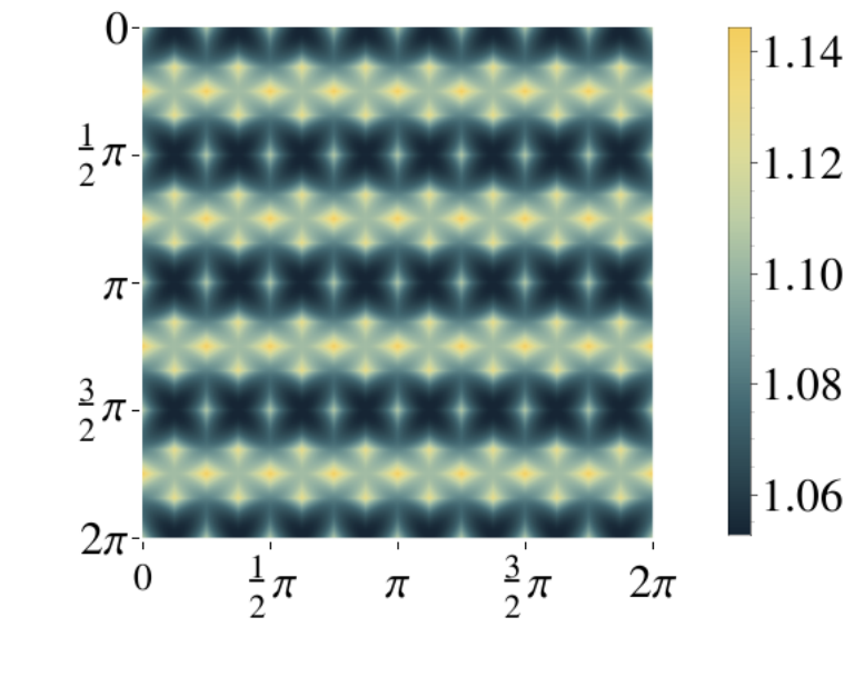
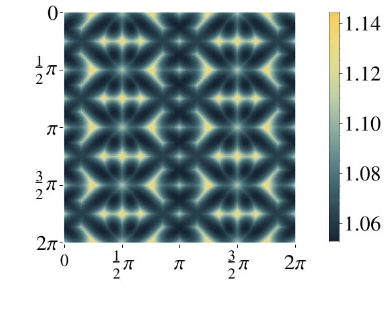
4.2 Optimisation of Bell inequalities for fixed measurement directions

In several applications a large violation is desirable. Given the experimental measurement setup used to evaluate a given Bell inequality, there might be different inequalities that lead to a higher violation. In that sense, they are ”better” inequalities. Finding an optimal inequality seems to be a difficult task. In some cases the methods above (Corollary 1 (1) and (2)) might give an intuition how to improve a given matrix of coefficients $g$ without changing the involved measurements.
There is another possible motivation for restricting the observables in the optimisation of the violation: It turns out that the average violation of Bell inequalities inside this restricted parameter space is larger than the one for the whole parameter space. Figure 2 shows the probability of an amount of violation for completely random coefficients and rotated versions (Corollary 1 (1)) of

g=\left(\begin{array}[]{ccc}1&-1&-1\\ 1&1&-1\\ 1&1&1\\ \end{array}\right).

(29)

Figure 2: A histogram of the maximal violation

\nu^{\prime}

of a random Bell inequality (light) and a “twisted” version of Gisin’s inequality [24] (dark). The size of the matrices is

3\times 3

. The random inequality has equally distributed coefficients in

[-1,1]

. For the other inequality, the rotation angles are equally distributed. The probability of a given violation is estimated from samples of

50000

inequalities each. The violation of the original inequality by Gisin is

\nu=1.2

Example 2.

The coefficients of Gisin’s inequality [24] for $M_{1}=M_{2}=6$ read

g=\left(\begin{array}[]{cccccc}1&-1&-1&-1&-1&-1\\ 1&1&-1&-1&-1&-1\\ 1&1&1&-1&-1&-1\\ 1&1&1&1&-1&-1\\ 1&1&1&1&1&-1\\ 1&1&1&1&1&1\\ \end{array}\right).

(30)

This inequality has $B=18$ , as one can easily see when the first two rows get multiplied with $-1$ . The quantum value is $T=M/\sin(\pi/(2M))=12\sqrt{2+\sqrt{3}}\approx 23.1822$ . Using Corollary 1 (2) we can optimise the coefficients numerically, and obtain

	$\displaystyle g^{\prime}$	$\displaystyle=$	$\displaystyle V\mbox{diag }(\|\|g\|\|_{2},\|\|g\|\|_{2},\|\|g\|\|_{2},\|\|g\|\|_{2},-\|\|g\|\|_{2},-\|\|g\|\|_{2})W^{T}$
		$\displaystyle=$	$\displaystyle(1+\sqrt{3})\left(\begin{array}[]{cccccc}0&0&-1&0&0&-1\\ 1&0&0&-1&0&0\\ 0&1&0&0&-1&0\\ 0&0&1&0&0&-1\\ 1&0&0&1&0&0\\ 0&1&0&0&1&0\\ \end{array}\right),$

which is equivalent to the CHSH inequality. This implies a violation of $\nu^{\prime}=\sqrt{2}$ and $B(g^{\prime})=6(1+\sqrt{3})\approx 16.3923$ . Here we ignored the condition in Eq (11) of Corollary 1 (2) as tightness of $T$ is ensured by the fact that all singular values are equal. One would obtain the same result, when considering $g^{\prime}=V\mbox{diag }(||g||_{2},||g||_{2},||g||_{2}-\varepsilon,||g||_{2}-\varepsilon,-||g||_{2}+\varepsilon,-||g||_{2}+\varepsilon)W^{T}$ for a very small positive $\varepsilon$ . In this way the degeneracy remains $d^{\prime}=2$ and the condition of Eq. (11) is fulfilled. The matrix $g^{\prime}$ constitutes a local optimum, i.e. small modifications of the singular values lead to a smaller violation.

Example 3 (Fishburn-Reeds Inequalities [16]).

In [16], the authors construct a series of inequalities with increasing number of measurement settings. For $d\in\mathds{N}$ greater or equal two,

g=V^{d}(V^{d})^{T}-\frac{4}{3}\mathds{1},

(38)

where $V^{d}$ is a $(d-1)d\times d$ matrix containing all rows of the form $(-1,0,...,0,1,0,...,0)$ and $(1,0,...,0,1,0,...)$ . The columns of $V^{d}$ are orthogonal and thus $\frac{1}{\sqrt{2(d-1)}}V^{d}$ , $(2(d-1)-4/3)\mathds{1}^{d}$ and $\frac{1}{\sqrt{2(d-1)}}V^{d}$ form a truncated singular value decomposition of $g$ . Therefore, the optimal measurement settings for party one and party two are identical. Intuitively, this choice of settings seems to be not optimal with respect to the amount of violation. We searched numerically for inequalities with a larger violation using methods (1) and (2) of Corollary 1. We give improved violations for $d=2,...,5$ in Table 1. Due to the computational complexity of determining $B$ , it is likely that the given values are not the maximal ones achievable with these methods.

$d$	$\nu=T/B$	$\nu^{\prime}=T/B^{\prime}$
$2$	$1$	$\sqrt{2}\approx 1.41421$
$3$	$4/3\approx 1.33333$	$1.34163$
$4$	$7/5=1.4$	$\sqrt{2}\approx 1.41421$
$5$	$10/7\approx 1.42857$	$1.42860$

Table 1: Optimized violations of the first four inequalities by Fishburn and Reeds [16],

T/B^{\prime}

, compared to the original violation

T/B

. The explicit coefficients of the corresponding matrix

g^{\prime}

are given in the supplemental material. Note that the given values for

\nu^{\prime}

are not necessarily maximal.

4.3 Optimisation of dimension witnessing Bell inequalities

The minimal $d^{\prime}$ for a solution $\alpha$ is a lower bound on the length of the vectors $\vec{v}_{i}$ and $\vec{w}_{j}$ , which is linked to the dimension of the observables. For example, if this minimal $d^{\prime}$ is larger than three, the maximal quantum value of the inequality cannot be reached using qubits. Let us denote the bound for $d^{\prime}$ -dimensional real vectors by $T_{d^{\prime}}$ . Please note that $B=T_{1}$ .
In the previous section, we aimed at increasing the ratio $T/T_{1}$ by decreasing $T_{1}$ . The same optimisations can be performed for any other value $d^{\prime}$ with $T_{d^{\prime}}<T$ .
To calculate the bound $T_{d^{\prime}}$ , we are interested in the optimal strategy (optimal ”observables”) achieving this bound. We note that the optimal observables of party two are fixed by the ones of party one. The maximum in Eq. (4) using Eq. (7) is achieved, if for all $x_{2}$ (each column), the vector $\vec{w}_{x_{2}}$ is parallel to $\sum_{x_{1}}g_{x_{1},x_{2}}\vec{v}_{x_{1}}$ , i.e.

\vec{w}_{x_{2}}=\frac{1}{||\sum g_{x_{1},x_{2}}\vec{v}_{x_{1}}||}\sum g_{x_{1},x_{2}}\vec{v}_{x_{1}},

(39)

so the bound simplifies to

T_{d^{\prime}}(g)=\max_{\vec{v}_{x_{1}}\in\mathds{R}^{d^{\prime}},||\vec{v}_{x_{1}}||=1}\sum_{x_{2}=1}^{M_{2}}\left|\left|\sum_{x_{1}=1}^{M_{1}}g_{x_{1},x_{2}}\vec{v}_{x_{1}}\right|\right|.

(40)

As $T_{d^{\prime}}(g)=T_{d^{\prime}}(g^{T})$ , we can assume that $M_{1}\leq M_{2}$ without loss of generality. We give an example for such optimisations:

Example 4.

We optimise inequality $D6_{1}$ in Ref. [25]. It is the skew left circulant matrix given by the first row $\left(\begin{array}[]{cccccc}1&0&1&0&1&1\end{array}\right)$ , i.e.

{D6}_{1}=\left(\begin{array}[]{cccccc}1&0&1&0&1&1\\ 0&1&0&1&1&-1\\ 1&0&1&1&-1&0\\ 0&1&1&-1&0&-1\\ 1&1&-1&0&-1&0\\ 1&-1&0&-1&0&-1\\ \end{array}\right)

(41)

A solution $\alpha$ of Theorem 1 is $\alpha=\sqrt{\frac{M}{d}}\mathds{1}^{d}$ , as it is the case for many circulant (left, right, skew left, skew right) matrices. See [26] for the singular value decomposition of circulant matrices. We applied modifications (1) and (2) of Corollary 1. We started with a global random search to find good starting points, which we further optimised by a local optimisation. Both algorithms are numerical. This led us to the matrix

g^{\prime}=\left(\begin{array}[]{cccccc}-0.350174&0.323788&0.344416&-0.368076&-0.299221&0.31404\\ -0.472675&-0.357842&-0.182589&-0.31764&-0.377403&0.215713\\ -0.218507&-0.300642&-0.525576&-0.185735&0.38952&0.279595\\ 0.39405&0.286377&-0.315566&-0.315986&0.296399&0.391561\\ 0.303896&0.37589&-0.193803&-0.514786&-0.310722&-0.200436\\ 0.190791&-0.355309&-0.321679&-0.184563&-0.326631&-0.511833\\ \end{array}\right),

(42)

which corresponds to an inequality with a qutrit to qubit ratio of $T/T_{3}\approx 1.02622$ . This seems to be small. However, we do not know of a higher ratio than $1.03528$ with few settings (see $\mathcal{B}_{X4}$ in [27], with $8+4$ settings).

5 Conclusions

We presented two modifications of the coefficients of bipartite CHSH-type Bell inequalities, which preserve tightness of the Tsirelson bound $T$ given in [22]. Physically, they do not affect the optimal observables (up to a relative rotation of the two laboratories). We applied this method to show that for any relative rotation of the two laboratories, there is a Bell inequality that is maximally violated for this rotation and a fixed shared quantum state. Furthermore we optimised Bell inequalities with respect to the ratio of the quantum value and the local hidden varible bound. Finally we showed how our method can be used to optimise dimension witnessing Bell inequalities, i.e. Bell inequalities, where the maximal quantum value is not achievable with two qubits.

We thank N. Gisin for discussions on [24]. This project was supported by the DFG, BMBF and SFF of Heinrich-Heine-University Düsseldorf.

References

[1] John Stewart Bell. On the Einstein Podolski Rosen Paradox. Physics, 1:195–200, 1964.
[2] A. Einstein, B. Podolsky, and N. Rosen. Can quantum-mechanical description of physical reality be considered complete? Phys. Rev., 47:777–780, May 1935.
[3] Alain Aspect, Philippe Grangier, and Gérard Roger. Experimental Realization of Einstein-Podolsky-Rosen-Bohm Gedankenexperiment: A New Violation of Bell’s Inequalities. Phys. Rev. Lett., 49:91–94, Jul 1982.
[4] Gregor Weihs, Thomas Jennewein, Christoph Simon, Harald Weinfurter, and Anton Zeilinger. Violation of bell’s inequality under strict einstein locality conditions. Phys. Rev. Lett., 81:5039–5043, Dec 1998.
[5] M. A. Rowe, D. Kielpinski, V. Meyer, C. A. Sackett, W. M. Itano, C. Monroe, and Wineland D.J. Experimental violation of a Bell’s inequality with efficient detection. Nature, 409:791–794, 2001.
[6] M. Ansmann, H. Wang, R. C. Bialczak, M. Hofheinz, E. Lucero, M. Neeley, A. D. O’Connell, D. Sank, M. Weides, J. Wenner, A. N. Cleland, and J. M. Martinis. Violation of Bell’s inequality in Josephson phase qubits. Nature, 461:504–506, September 2009.
[7] B. G. Christensen, K. T. McCusker, J. B. Altepeter, B. Calkins, T. Gerrits, A. E. Lita, A. Miller, L. K. Shalm, Y. Zhang, S. W. Nam, N. Brunner, C. C. W. Lim, N. Gisin, and P. G. Kwiat. Detection-Loophole-Free Test of Quantum Nonlocality, and Applications. Phys. Rev. Lett., 111:130406, Sep 2013.
[8] Peter Shadbolt, Tamás Vértesi, Yeong-Cherng Liang, Cyril Branciard, Nicolas Brunner, and Jeremy L. O’Brien. Guaranteed violation of a Bell inequality without aligned reference frames or calibrated devices. Sci. Rep., 2, jun 2012.
[9] C. Erven, E. Meyer-Scott, K. Fisher, J. Lavoie, B. L. Higgins, Z. Yan, C. J. Pugh, J.-P. Bourgoin, R. Prevedel, L. K. Shalm, L. Richards, N. Gigov, R. Laflamme, G. Weihs, T. Jennewein, and K. J. Resch. Experimental Three-Particle Quantum Nonlocality under Strict Locality Conditions. ArXiv e-prints, September 2013.
[10] B. P. Lanyon, M. Zwerger, P. Jurcevic, C. Hempel, W. Dür, H. J. Briegel, R. Blatt, and C. F. Roos. Experimental violation of multipartite Bell inequalities with trapped ions. ArXiv e-prints, December 2013.
[11] A. Ekert. Quantum cryptography based on Bell’s theorem. Physical Review Letters, 67(6):661–663, 1991.
[12] H. Buhrman, O. Regev, G. Scarpa, and R. de Wolf. Near-Optimal and Explicit Bell Inequality Violations. ArXiv e-prints, December 2010.
[13] M. Junge and C. Palazuelos. Large Violation of Bell Inequalities with Low Entanglement. Communications in Mathematical Physics, 306(3):695–746, 2011.
[14] Q. Y. He, E. G. Cavalcanti, M. D. Reid, and P. D. Drummond. Testing for Multipartite Quantum Nonlocality Using Functional Bell Inequalities. Phys. Rev. Lett., 103:180402, Oct 2009.
[15] Wei-Bo Gao, Xing-Can Yao, Ping Xu, He Lu, Otfried Gühne, Adán Cabello, Chao-Yang Lu, Tao Yang, Zeng-Bing Chen, and Jian-Wei Pan. Bell inequality tests of four-photon six-qubit graph states. Phys. Rev. A, 82:042334, Oct 2010.
[16] PC Fishburn and JA Reeds. Bell inequalities, Grothendieck’s constant, and root two. SIAM J. Discrete Math., 7(1):48–56, 1994.
[17] Otfried Gühne and Adán Cabello. Generalized Ardehali-Bell inequalities for graph states. Phys. Rev. A, 77:032108, Mar 2008.
[18] JF Clauser, MA Horne, A Shimony, and RA Holt. Proposed experiment to test local hidden-variable theories. Phys. Rev. Lett., 23(15):880–884, 1969.
[19] R. F. Werner and M. M. Wolf. Bell inequalities and entanglement. Quant. Inform. Comput., 1:1–25, 2001.
[20] Asher Peres. Existence of a free will as a problem of physics. Foundations of Physics, 16(6):573–584, 1986.
[21] B.S. Cirel’son. Quantum generalizations of Bell’s inequality. Lett. Math. Phys, 4:93–100, 1980.
[22] Michael Epping, Hermann Kampermann, and Dagmar Bruß. Designing Bell Inequalities from a Tsirelson Bound. Phys. Rev. Lett., 111:240404, Dec 2013.
[23] BS Tsirelson. Some results and problems on quantum Bell-type inequalities. Hadronic J., 8(4):329–345, 1993.
[24] N Gisin. Bell inequality for arbitrary many settings of the analyzers. Phys. Lett. A, 260(September):8–10, 1999.
[25] N. Gisin. Bell inequalities: many questions, a few answers. In essays in honour of Abner Shimony, Eds Wayne C. Myrvold and Joy Christian, The Western Ontario Series in Philosophy of Science, pages 125–140, 2009.
[26] Herbert Karner, Josef Schneid, and Christoph W Ueberhuber. Spectral decomposition of real circulant matrices. Linear Algebra and its Applications, 367(0):301 – 311, 2003.
[27] Tamás Vértesi and Károly Pál. Bounding the dimension of bipartite quantum systems. Phys. Rev. A, 79(4):042106, April 2009.

Optimisation of Bell inequalities with invariant Tsirelson bound

Abstract

1 Introduction

2 A subclass of CHSH-type Bell inequalities

Theorem 1 (Tightness of TT [22]).

3 Modifying Bell inequalities inside this class

Corollary 1.

Proof.

4 Using these modifications as a method

4.1 Maximally violated Bell inequality for relative rotation of laboratories

Example 1.

4.2 Optimisation of Bell inequalities for fixed measurement directions

Example 2.

Example 3 (Fishburn-Reeds Inequalities [16]).

4.3 Optimisation of dimension witnessing Bell inequalities

Example 4.

5 Conclusions

References

References

Theorem 1 (Tightness of $T$ [22]).