A Rate-Distortion Approach to Index Coding

We consider a general version of the index coding problem, in which a single encoder observes a vector-valued source, the components of which are i.i.d., uniformly-distributed, binary random variables. There are several decoders, each of which has a subset of the source components as side information, and seeks to losslessly reproduce a disjoint subset of source components. The encoder must broadcast a single message to all of the decoders, which allows all of them to reproduce their desired source components. This problem models media distribution over a rate-constrained downlink in which some of the clients already have some of the media to be distributed, which can happen if they cached prior transmissions from the encoder. We seek to understand what rate is required of the encoder’s message when the encoder may code over many i.i.d. realizations of the source vector. Specifically, we seek estimates of the minimal rate that are both efficiently computable and provably close to the true minimal rate, at least under some conditions.

The index coding problem has attracted considerable attention since it was introduced (e.g., [1, 2, 3, 4, 5, 6, 7, 8]), and the formulations studied vary along at least three different axis. First, one can impose structure on the demands and the side information. Birk and Kol’s paper [1] introducing the problem focused on the case in which each source bit is demanded by exactly one decoder, and if Decoder $i$ has Decoder $j$’s demand as side information then Decoder $j$ must have Decoder $i$’s demand as side information. The problem instance can then be represented as an undirected graph, with the nodes representing the source bits (or equivalently, the decoders) and the edges representing the side information pattern. Slightly more generally, one can relax the symmetry assumption to obtain a directed, instead of undirected, graph. Shanmugam et al. [4] call this unicast index coding. We shall consider here the more general version in which each decoder can demand any number of source components and the demands may be overlapping among the decoders. Shanmugam et al. call this groupcast index coding; we shall simply call it index coding.

A second independent axis along which index coding formulations vary is whether one allows for coding over time (vector codes) or whether the code must operate on each time instant separately (scalar codes). We shall focus on the former here, due to its intrinsic importance and its connection with rate-distortion theory. Third, and finally, some works require the decoders to reproduce their demands with zero error [2, 4, 5, 6, 9] while others require that the block-error probability vanish [7, 8]. Yet another possibility is to require that the bit-error probability vanish. This paper shall focus on the latter two.

Irrespective of the formulation, most work on index coding views the problem graph-theoretically [3, 4, 9], as in Birk and Kol’s original paper. One can then lower and upper bound the optimal rate using graph-theoretic quantities such as the independence number, the clique-cover number, fractional clique-cover number (e.g. [5]), the min-rank [2] and others [3, 4, 9]. This approach has proven to be successful for showing the utility of coding over blocks for this problem [10], and for showing the utility of nonlinear codes [11]. Many of these graph-theoretic quantities are known to be NP-hard to compute, however, and for the others there is no apparent polynomial-time algorithm. Thus these bounds are only useful theoretically or when numerically solving small examples. A noteworthy exception is Theorem 2 of Blasiak et al., which provides a polynomial-time-computable bound that is within a nontrivial factor of the optimal rate for arbitrary instances. The factor in question is quite large, however.

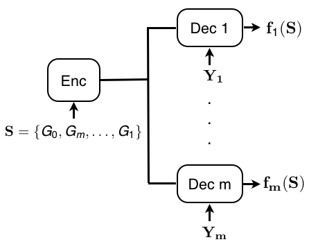
We approach index coding as a special case of the problem of lossy compression with a single encoder and multiple decoders, each with side information. This more general problem was introduced by Heegard-Berger [12] (but see Kaspi [13]) and is sometimes referred to as the Heegard-Berger problem. Index coding can be viewed as the special case in which the source, at each time, is a vector of i.i.d. uniform bits, the side information of each decoder consists of a subset of the source bits, and the distortion measure for Decoder $i$ is the Hamming distortion between the subset of the source bits that Decoder $i$ seeks to reproduce and Decoder $i$’s reproduction of that subset. We then consider the minimum rate possible so that all of the decoders can achieve zero distortion.

Viewing the problem in this way allows us to apply tools from network information theory, such as random coding techniques, binning, the use of auxiliary random variables, etc. Using this approach, we prove two achievable bounds and an impossibility (or “converse”) bound. Both of the achievable bounds are built upon the best known achievable bound for the Heegard-Berger problem, which is due to Timo et al. [14]. The Timo et al. scheme involves an optimization over the joint distribution of a large number of auxiliary random variables; we provide two methods for selecting this distribution, the first of which is polynomial-time computable but only yields integer rate bounds, while the second is more complex but can yield fractional rates. The achievability results in this paper are thus unusual in that the emphasis is on algorithms for selecting the joint distribution of auxiliary random variables rather than proving new coding theorems per se. It is worth noting that the Timo et al. result is representative of many achievability results in network information theory that take the form of optimization problems over the joint distribution of auxiliary random variables (e.g., [15]). The task of solving these optimization problems has received little attention in the literature.¹¹ 1 Indeed, the prospect that some of these “single-letter” optimization problems might be intrinsically hard to compute is intriguing and seemingly unexplored (though see Arikan [16]).

Our impossibility result is related to the “degraded-same-marginals” (DSM) impossibility result for broadcast channels [17, 18]. The idea is that the optimal rate can be computed exactly when the source $S$ and the side information variables $Y_{1},\ldots,Y_{m}$ can be coupled in such a way that

meaning that the random variables form a Markov chain in this order, where $\sigma(\cdot)$ is an arbitrary permutation [14]. We call such an instance one with degraded side information. One may then lower bound a given problem by providing (for example), $Y_{1}$ to Decoder 2, $Y_{1}$ and $Y_{2}$ to Decoder 3, etc., to form a degraded instance whose optimal rate is only lower than that of the original problem. We provide a lower bound in this spirit for the general Heegard-Berger problem that improves somewhat on that obtained via a direct application of the above technique. As such, we shall call it the DSM+ lower bound. When applied to the index coding problem, the DSM+ bound provides the same conclusion as a lower bound due to Blasiak et al., although under slightly weaker hypotheses.

We use the DSM+ lower bound to show that our low-complexity achievable bound equals the optimal rate for any number of source components, so long as the number of decoders does not exceed three.²² 2 Recall that we allow each decoder to demand more than one source component and each source component to be demanded by more than one decoder. In fact, we show the more general result that the achievable bound equals the optimal rate for any number of source components and any number of decoders so long as each source component is present as side information at all of the decoders, none of the decoders, all but one of the decoders, or all but two of the decoders. It is apparent that every problem with three or fewer decoders must be of this form. We also show that the achievable bound coincides with the optimal rate when none of the source components are “excess,” a concept that plays an important role in our achievable scheme and that shall be defined later. Our low-complexity achievable scheme bears some resemblance to the partition multicast scheme of Tehrani, Dimakis, and Neely [6]. Although our scheme does not subsume partition multicast (which is NP-hard to compute [6]), we do show that it is optimal in all explicit instances of the problem for which Tehrani, Dimakis, and Neely show that partition multicast is optimal.³³ 3 Tehrani et al. also show that partition multicast is optimal for the implicitly-defined class of instances for which clique cover is optimal.

Although the paper is focused mainly on index coding, the results herein also have some significance for the Heegard-Berger problem. The DSM+ bound, mentioned earlier, is the best general lower bound for this problem, and our conclusive results for the index problem represent some of the few nondegraded instances of the Heegard-Berger problem for which the optimal rate is known (see [19, 20, 21, 22, 23, 24] others). This paper is also the first work that considers algorithms for selecting the distribution of the auxiliary random variables in the Timo et al. scheme.

As noted earlier, this work differs from much of the literature on index coding by approaching the problem as one of rate-distortion, or source coding. Some recent works have also approached the problem as one of channel coding [7, 8], and in particular, interference alignment. One of the advantages of the source coding approach espoused here is that it can readily accommodate richer source models and distortion constraints, including sources with memory, lossy reconstruction of analog sources, etc. The very formulation of index coding presumes that the sources have already been compressed down to i.i.d. uniform bits. Thus the index coding is “separated” from the underlying compression, when in fact there might be some advantage to combining the two, a topic that we shall consider in subsequent work.

This paper is outlined as follows. Section II formulates the Heegard-Berger problem and Section III provides the DSM+ lower bound for it. Section IV formulates the index coding problem. Section V and VI provide a lower bound and an upper bound for the problem respectively. Section VII describes our first scheme of index coding, and Section VIII provides several optimality results for this scheme, including our results for three decoders. Section IX describes our second scheme.

We begin by considering the general form of the Heegard-Berger problem, as opposed to the index-coding problem in particular. There is a single encoder with source ${S}$ and there are $m$ decoders. Decoder $i$ has a side information ${Y_{i}}$ that in general depends on ${S}$. The encoder sends a message at rate $R$ to the decoders, and Decoder $i$ wishes to reconstruct the source with a given distortion constraint $D_{i}$. The objective is to find the rate distortion tradeoff for this problem setup. This is made precise via the following definitions.

Finding a computable characterization $R(D)$ is a long-standing open problem in network information theory. Currently, such a characterization is only available for a few special cases. Heegard and Berger themselves [12] provided one when the side information at the decoders is degraded. Watanabe [19] provided one for the case that the source consists of two independent components, the distortion constraints for both decoders are decoupled across the two components, and the side information at the two decoders is degraded “in mismatched order” (see [19] for the precise setup). Sgarro’s result [22] implies a characterization for the problem in which two decoders both wish to reproduce the source losslessly, without any assumption on their side information (see also [23]). Timo et al. [24] provide a characterization for the two-decoder case when one decoder’s side information is “conditionally less noisy” than the other’s and the weaker decoder seeks to losslessly reproduce a deterministic function of the source. Timo et al. [20] solve various two-decoder cases in which the source consists of two components, say $(X,Y)$, and one decoder has $X$ as side information and wants to reconstruct $Y$ while the other has $Y$ as side information and wants to reconstruct $X$. The present authors determined the rate distortion region for the two-decoder problem with vector Gaussian sources and side information, subject to a constraint on the error covariance matrices at the two decoders [21]. Several (nondegraded) special cases in which both decoders wish to losslessly reproduce a function of the source have been solved by Laich and Wigger [25]. Of course, several instances of index coding that are not degraded have also been solved.

A general achievable result, i.e., an upper bound on $R(D)$, was provided by Heegard and Berger [12], which was corrected and extended by Timo et al. [14]. We provide a computable lower bound on $R(D)$ for general instances of the problem in this section. This lower bound will be used later in the paper to solve several index coding instances.

We start our analysis by providing a lower bound to the general rate distortion problem.

The idea behind the proof was described in the introduction. Note that since the optimal rate only depends on the source and side information through the “marginals”

we may couple the $Y_{i}$ variables to form a joint distribution $\bar{P}(S,Y_{1},\ldots,Y_{m})$ as we please, leading to the inner optimization in (1). Also note that a direct application of the DSM idea would yield the weaker bound in which $\cup_{j\leq i}Y_{\sigma(j)}$ appears as an argument to $g_{\sigma(i)}$ in (3).

Next, we turn our focus to the index coding problem which can be viewed as a special case of the Heegard-Berger problem.

For the $m$ user index coding problem, each decoder $\alpha$ wants to reconstruct $\mathbf{f_{\alpha}}$, which is an arbitrary subset of the source $\mathbf{S}$, that is, a collection of i.i.d. Bernoulli($\frac{1}{2}$) bits at the encoder. There may be overlapping demands, i.e., more than one decoder may demand the same bit. Also, each Decoder $\alpha$ has side information $\mathbf{Y_{\alpha}}$ consisting of an arbitrary subset of the source. We assume that decoders do not demand a component of their own side information since they already have it, and we assume that $\mathbf{Y_{\alpha}}\neq\mathbf{Y_{\beta}}$, for all $\alpha\neq\beta$ since we can combine two decoders if they have the same side information. We may also assume that every source bit is demanded by at least one decoder, for otherwise that bit may be completely purged from the system.

Let $\mathbf{S_{J}}$ denote the part of the source which each decoder in a subset $J$ of $[m]$ does not have and all decoders in $[m]\backslash J$ have as side information. If $J=\{\alpha\}$, i.e., a singleton, then for ease of notation we use $\mathbf{S_{\alpha}}$ instead of $\mathbf{S_{\{\alpha\}}}$. Since there are $m$ decoders, we group the elements of $\mathbf{S}$ into $2^{m}$ disjoint sets such that $\mathbf{S}=\cup_{J\subseteq[m]}\mathbf{S_{J}}$. Note that each $\mathbf{S_{J}}$ may be empty, may consist of a single bit, or may consist of multiple bits.

Let $G_{0}=\mathbf{S_{[m]}}$ denote the elements of the source that none of the decoders have, $G_{m}=\mathbf{S_{\emptyset}}$ denote the elements all decoders have, $G_{m-1}=\cup_{\alpha\in[m]}\mathbf{S_{\alpha}}$ denote elements that $m-1$ of the decoders have, $G_{m-2}=\cup_{\tiny\begin{aligned} &\{\alpha,\beta\}\subseteq[m]\\ &\alpha\neq\beta\end{aligned}}\mathbf{S_{\{\alpha,\beta\}}}$ denote elements that $m-2$ of the decoders have and so on. To ease the notation for the rest of the paper, whenever we write a set $\{\alpha,\beta\}$, we assume $\alpha\neq\beta$ unless otherwise stated. Then $\mathbf{S}$ can be represented as $\mathbf{S}=\{G_{0},G_{m},G_{m-1},\ldots,G_{1}\}$, as shown in Fig. 1.

The demand $\mathbf{f_{\alpha}}$ at Decoder $\alpha$ can be written in terms of components $\mathbf{S_{J}}$ of $\mathbf{S}$. For this, we introduce the following notation.

Let $f_{IJ}$ denote the demand that is a subset of source $\mathbf{S_{J}}$ and is required by each decoder in a subset $I$ of $[m]$ and by no decoders in $[m]\backslash I$. If $I=\{\alpha\}$, then for ease of notation we use $f_{\alpha J}$ instead of $f_{\{\alpha\}J}$. We will generally assume that $I\subseteq J$ since only decoders in $J$ may have a demand about $\mathbf{S_{J}}$ and decoders in $[m]\backslash J$ already have $\mathbf{S_{J}}$ as side information. If $I\not\subseteq J$, $f_{IJ}$ is empty. Also, $f_{IJ}$ and $f_{KJ}$ are independent (i.e., $f_{IJ}\perp f_{KJ}$) for all possible choices of $I$, $K$ and $J$ with $I\neq K$ since $f_{IJ}\cap f_{KJ}=\emptyset$ unless $I=K$. Lastly, each $f_{IJ}$ may be empty, a single bit or may consist of multiple bits.

We have written the source as $\mathbf{S}=\{G_{0},G_{m},G_{m-1}$, $\ldots,G_{1}\}$ and the demands in terms of $\mathbf{S_{J}}$’s. From now on, we consider an ordered set structure on $\mathbf{S}$ which naturally induces orders on $\mathbf{S_{J}}$’s. Then each demand $f_{IJ}$ is also an ordered set that can also be viewed as a vector. In fact, we shall find it convenient to view $f_{IJ}$, $\mathbf{S}$, and other similar quantities at times as sets and at times as vectors.

Since this problem can be considered as a special case of the Heegard-Berger problem, we use a similar definition for the code except for the distortion. Specifically, we consider block error probabilities instead of the distortion constraints stated in Definition 1. Hence, we use the following definitions for the code, error and optimal rate.

Then achievability and optimal rate can be defined as follows.

We shall call the problem defined in this section index coding, although most existing work on index coding requires the code to achieve zero, as opposed to vanishing, block error [4, 5, 6]. In support of the definitions adopted here, see [7, 8] for works that use vanishing block error probability and [26] for results connecting the two formulations.

The next theorem gives a lower bound to the index coding problem using the DSM+ lower bound from Section III.

References

• [1] Y. Birk and T. Kol, “Informed-source coding-on-demand (iscod) over broadcast channels,” in INFOCOM ’98. Seventeenth Annual Joint Conference of the IEEE Computer and Communications Societies. Proceedings. IEEE, vol. 3, 1998, pp. 1257–1264 vol.3.
• [2] Z. Bar-Yossef, Y. Birk, T. S. Jayram, and T. Kol, “Index coding with side information,” in Foundations of Computer Science, 2006. FOCS ’06. 47th Annual IEEE Symposium on, 2006, pp. 197–206.
• [3] K. Shanmugam, A. Dimakis, and M. Langberg, “Local graph coloring and index coding,” in Information Theory Proceedings (ISIT), 2013 IEEE International Symposium on, July 2013, pp. 1152–1156.
• [4] K. Shanmugam, A. G. Dimakis, and M. Langberg, “Graph theory versus minimum rank for index coding,” in Information Theory (ISIT), 2014 IEEE International Symposium on, June 2014, pp. 291–295.
• [5] A. Blasiak, R. Kleinberg, and E. Lubetzky, “Broadcasting with side information: Bounding and approximating the broadcast rate,” Information Theory, IEEE Transactions on, vol. 59, no. 9, pp. 5811–5823, 2013.
• [6] A. Tehrani, A. Dimakis, and M. Neely, “Bipartite index coding,” in Information Theory Proceedings (ISIT), 2012 IEEE International Symposium on, July 2012, pp. 2246–2250.
• [7] H. Maleki, V. Cadambe, and S. Jafar, “Index coding ;an interference alignment perspective,” Information Theory, IEEE Transactions on, vol. 60, no. 9, pp. 5402–5432, Sept 2014.
• [8] F. Arbabjolfaei, B. Bandemer, Y.-H. Kim, E. Sasoglu, and L. Wang, “On the capacity region for index coding,” in Information Theory Proceedings (ISIT), 2013 IEEE International Symposium on, July 2013, pp. 962–966.
• [9] F. Arbabjolfaei and Y.-H. Kim, “Local time sharing for index coding,” in Information Theory (ISIT), 2014 IEEE International Symposium on, June 2014, pp. 286–290.
• [10] N. Alon, E. Lubetzky, U. Stav, A. Weinstein, and A. Hassidim, “Broadcasting with side information,” in Foundations of Computer Science, 2008. FOCS ’08. IEEE 49th Annual IEEE Symposium on, 2008, pp. 823–832.
• [11] E. Lubetzky and U. Stav, “Nonlinear index coding outperforming the linear optimum,” Information Theory, IEEE Transactions on, vol. 55, no. 8, pp. 3544–3551, 2009.
• [12] C. Heegard and T. Berger, “Rate distortion when side information may be absent,” Information Theory, IEEE Transactions on, vol. 31, no. 6, pp. 727–734, 1985.
• [13] A. H. Kaspi, “Rate-distortion function when side-information may be present at the decoder,” Information Theory, IEEE Transactions on, vol. 40, no. 6, pp. 2031–2034, 1994.
• [14] R. Timo, T. Chan, and A. Grant, “Rate distortion with side-information at many decoders,” Information Theory, IEEE Transactions on, vol. 57, no. 8, pp. 5240–5257, 2011.
• [15] A. E. Gamal and Y.-H. Kim, Network Information Theory. New York, NY, USA: Cambridge University Press, 2012.
• [16] E. Arikan, “Some complexity results about packet radio networks,” Information Theory, IEEE Transactions on, vol. 30, no. 4, pp. 681–685, 1984.
• [17] S. Vishwanath, G. Kramer, S. Shamai, S. Jafar, and A. Goldsmith, “Capacity bounds for Gaussian vector broadcast channels,” DIMACS SERIES IN DISCRETE MATHEMATICS AND THEORETICAL COMPUTER SCIENCE, vol. 62, pp. 107–122, 2004.
• [18] P. Vishwanath and D. Tse, “On the capacity of the multiple antenna broadcast channel,” DIMACS SERIES IN DISCRETE MATHEMATICS AND THEORETICAL COMPUTER SCIENCE, vol. 62, pp. 87–106, 2004.
• [19] S. Watanabe, “The rate-distortion function for product of two sources with side-information at decoders,” Information Theory, IEEE Transactions on, vol. 59, no. 9, pp. 5678–5691, Sept 2013.
• [20] R. Timo, A. Grant, and G. Kramer, “Lossy broadcasting with complementary side information,” Information Theory, IEEE Transactions on, vol. 59, no. 1, pp. 104–131, 2013.
• [21] S. Unal and A. B. Wagner, “Vector Gaussian rate-distortion with variable side information,” in Information Theory Proceedings (ISIT), 2014 IEEE International Symposium on, 2014.
• [22] A. Sgarro, “Source coding with side information at several decoders,” Information Theory, IEEE Transactions on, vol. 23, no. 2, pp. 179–182, 1977.
• [23] R. Timo, A. Grant, T. Chan, and G. Kramer, “Source coding for a simple network with receiver side information,” in Information Theory Proceedings (ISIT), 2008 IEEE International Symposium on, 2008, pp. 2307–2311.
• [24] R. Timo, T. J. Oechtering, and M. Wigger, “Source coding problems with conditionally less noisy side information,” Information Theory, IEEE Transactions on, vol. 60, no. 9, pp. 5516–5532, 2014.
• [25] T. Laich and M. Wigger, “Utility of encoder side information for the lossless Kaspi/Heegard-Berger problem,” in Information Theory Proceedings (ISIT), 2013 IEEE International Symposium on, 2013, pp. 3065–3069.
• [26] M. Langberg and M. Effros, “Network coding: Is zero error always possible?” in Communication, Control, and Computing (Allerton), 2011 49th Annual Allerton Conference on, Sept 2011, pp. 1478–1485.
• [27] S. Unal and A. B. Wagner, “A rate-distortion approach to index coding,” in ITA. IEEE, 2014, pp. 1–5.
• [28] M. Neely, A. Tehrani, and Z. Zhang, “Dynamic index coding for wireless broadcast networks,” Information Theory, IEEE Transactions on, vol. 59, no. 11, pp. 7525–7540, Nov 2013.
• [29] M. Maddah-Ali and U. Niesen, “Fundamental limits of caching,” Information Theory, IEEE Transactions on, vol. 60, no. 5, pp. 2856–2867, May 2014.
• [30] M. A. Maddah-Ali and U. Niesen, “Decentralized caching attains order-optimal memory-rate tradeoff,” CoRR, vol. abs/1301.5848, 2013.
• [31] R. T. Rockafellar, Convex Analysis. Princeton University Press, 1970.
Appendix
Lemma 4.
The minimum in (2) is unaffected by the presence of the cardinality bounds in condition 5).
Proof.
Without loss of generality let σ⁡(i)=i\sigma(i)=i for all i∈[m]i\in[m]. Let PU1,…,Um,S​(u1,…,um,s)P_{U_{1},\ldots,U_{m},{S}}(u_{1},\ldots,u_{m},s) denote the joint distribution of (U1,…,Um,S)(U_{1},\ldots,U_{m},{S}). We follow a procedure similar to that of [19]. First we find the bound on the cardinality of U1U_{1}, then U2U_{2}, etc.
To begin with, we consider the following (|𝒮|−1)+1+m(|\mathcal{S}|-1)+1+m functions of PU2,…,Um,S|U1(.,…,.|u1)P_{U_{2},\ldots,U_{m},{S}|U_{1}}(.,\ldots,.|u_{1}), denoted as gs0,s∈|𝒮|−1g^{0}_{s},s\in|\mathcal{S}|-1 and gl​o0,gd10,…,gdm0g^{0}_{lo},g^{0}_{d_{1}},\ldots,g^{0}_{d_{m}}.
gs0(PU2,…,Um,S|U1(.,…,.|u1))=∑u2,…,umPU2,…,Um,S|U1(u2,…,um,s|u1),\displaystyle g^{0}_{s}(P_{U_{2},\ldots,U_{m},{S}|U_{1}}(.,\ldots,.|u_{1}))=\sum_{u_{2},\ldots,u_{m}}P_{U_{2},\ldots,U_{m},{S}|U_{1}}(u_{2},\ldots,u_{m},s|u_{1}), (49)
for s=1,…,|𝒮|−1s=1,\ldots,|\mathcal{S}|-1 and
gl​o0(PU2,…,Um,S|U1(.,…,.|u1))\displaystyle g^{0}_{lo}(P_{U_{2},\ldots,U_{m},{S}|U_{1}}(.,\ldots,.|u_{1}))
=H(S|Y1)−H(S|U1=u1,Y1)+I(S;U2|U1=u1,Y1,Y2)+⋯+I(S;Um|U1=u1,…,U(m−1),Y1,…,Ym),\displaystyle=H({S}|{Y_{1}})-H({S}|U_{1}=u_{1},{Y_{1}})+I({S};U_{2}|U_{1}=u_{1},{Y_{1}},{Y_{2}})+\cdots+I({S};U_{m}|U_{1}=u_{1},\ldots,U_{(m-1)},{Y_{1}},\ldots,{Y_{m}}), (50)
and
gd10(PU2,…,Um,S|U1(.,…,.|u1))=𝔼[d(S,g1(u1,Y1))|U1=u1]\displaystyle g^{0}_{d_{1}}(P_{U_{2},\ldots,U_{m},{S}|U_{1}}(.,\ldots,.|u_{1}))=\mathbb{E}[d({S},g_{1}(u_{1},{Y}_{1}))|U_{1}=u_{1}]
gdm0(PU2,…,Um,S|U1(.,…,.|u1))=𝔼[d(S,gm(Um,Ym))|U1=u1]\displaystyle g^{0}_{d_{m}}(P_{U_{2},\ldots,U_{m},{S}|U_{1}}(.,\ldots,.|u_{1}))=\mathbb{E}[d({S},g_{m}(U_{m},{Y}_{m}))|U_{1}=u_{1}]
Then by Carathéodory’s theorem [31, Theorem 17.1] we can find a random variable U11U^{1}_{1} with |U11|≤|𝒮|+m+1|U^{1}_{1}|\leq|\mathcal{S}|+m+1 and random variables U21,…,Um1U^{1}_{2},\ldots,U^{1}_{m} where PU11,…,Um1,S​(u1,…,um,s)P_{U^{1}_{1},\ldots,U^{1}_{m},{S}}(u_{1},\ldots,u_{m},s) =PU11​(u1)​PU2,…,Um,S|U1​(u2,…,um,s|u1)=P_{U_{1}^{1}}(u_{1})P_{U_{2},\ldots,U_{m},{S}|U_{1}}(u_{2},\ldots,u_{m},s|u_{1}) such that from (49) PSP_{{S}} is preserved and from (50)
I(S;U11|Y1)+I(S;U21|U11,Y1,Y2)+⋯+I(S;Um1|U11,…,U(m−1)1,Y1,…,Ym)\displaystyle I({S};U^{1}_{1}|{Y_{1}})+I({S};U^{1}_{2}|U^{1}_{1},{Y_{1}},{Y_{2}})+\cdots+I({S};U^{1}_{m}|U^{1}_{1},\ldots,U^{1}_{(m-1)},{Y_{1}},\ldots,{Y_{m}})
=I(S;U1|Y1)+I(S;U2|U1,Y1,Y2)+I(S;Um|U1,…,U(m−1),Y1,…,Ym),\displaystyle=I({S};U_{1}|{Y_{1}})+I({S};U_{2}|U_{1},{Y_{1}},{Y_{2}})+I({S};U_{m}|U_{1},\ldots,U_{(m-1)},{Y_{1}},\ldots,{Y_{m}}),
and we have
𝔼[d(S,g1(U11,Y1)]=𝔼[d(S,g1(U1,Y1))]\displaystyle\mathbb{E}[d({S},g_{1}(U^{1}_{1},{Y}_{1})]=\mathbb{E}[d({S},g_{1}(U_{1},{Y}_{1}))]
𝔼[d(S,gm(Um1,Y1)]=𝔼[d(S,gm(Um,Y1))].\displaystyle\mathbb{E}[d({S},g_{m}(U^{1}_{m},{Y}_{1})]=\mathbb{E}[d({S},g_{m}(U_{m},{Y}_{1}))].
Now we consider the following |U1|​|𝒮|+(m−1)|U_{1}||\mathcal{S}|+(m-1) functions of PU11,U31,…,Um1,S|U21(.,…,.|u2)P_{U_{1}^{1},U^{1}_{3},\ldots,U^{1}_{m},{S}|U^{1}_{2}}(.,\ldots,.|u_{2}).
gs1(PU11,U31,…,Um1,S|U11(.,…,.|u2))=∑u3,…,umPU11,U31,…,Um1,S|U21(.,…,.|u2),\displaystyle g^{1}_{s}(P_{U_{1}^{1},U^{1}_{3},\ldots,U^{1}_{m},{S}|U^{1}_{1}}(.,\ldots,.|u_{2}))=\sum_{u_{3},\ldots,u_{m}}P_{U_{1}^{1},U^{1}_{3},\ldots,U^{1}_{m},{S}|U^{1}_{2}}(.,\ldots,.|u_{2}), (51)
for (u1,s)=1,…,|U1|​|𝒮|−1(u_{1},s)=1,\ldots,|{U_{1}}||\mathcal{S}|-1 and
gl​o1(PU11,U31,…,Um1,S|U21(.,…,.|u2))\displaystyle g^{1}_{lo}(P_{U_{1}^{1},U^{1}_{3},\ldots,U^{1}_{m},{S}|U^{1}_{2}}(.,\ldots,.|u_{2}))
=−H(S|U11,U21=u2,Y1,Y2)+I(S;U31|U11,U21=u2,Y1,Y2,Y3)⋯\displaystyle=-H({S}|U^{1}_{1},U^{1}_{2}=u_{2},{Y_{1}},{Y_{2}})+I({S};U^{1}_{3}|U^{1}_{1},U^{1}_{2}=u_{2},Y_{1},Y_{2},Y_{3})\cdots
+I(S;Um1|U11,U21=u2,U31…,U(m−1)1,Y1,…,Ym),\displaystyle\quad+I({S};U^{1}_{m}|U^{1}_{1},U^{1}_{2}=u_{2},U^{1}_{3}\ldots,U^{1}_{(m-1)},{Y_{1}},\ldots,{Y_{m}}), (52)
gd21(PU11,U31,…,Um1,S|U21(.,…,.|u2))=𝔼[d(S,g2(u2,Y2)|U21=u2]\displaystyle g^{1}_{d_{2}}(P_{U_{1}^{1},U^{1}_{3},\ldots,U^{1}_{m},{S}|U^{1}_{2}}(.,\ldots,.|u_{2}))=\mathbb{E}[d({S},g_{2}(u_{2},{Y}_{2})|U^{1}_{2}=u_{2}]
gdm1(PU11,U31,…,Um1,S|U21(.,…,.|u2))=𝔼[d(S,gm(Um1,Ym)|U21=u2].\displaystyle g^{1}_{d_{m}}(P_{U_{1}^{1},U^{1}_{3},\ldots,U^{1}_{m},{S}|U^{1}_{2}}(.,\ldots,.|u_{2}))=\mathbb{E}[d({S},g_{m}(U^{1}_{m},{Y}_{m})|U^{1}_{2}=u_{2}].
Again by Carathéodory’s theorem, there is a random variable U22U^{2}_{2} with |U22|≤|U1|​|𝒮|+m|U^{2}_{2}|\leq|U_{1}||\mathcal{S}|+m and random variables U32,…,Um2U^{2}_{3},\ldots,U^{2}_{m} where PU11,U22,…,Um2,S​(u1,…,um,s)P_{U_{1}^{1},U^{2}_{2},\ldots,U^{2}_{m},{S}}(u_{1},\ldots,u_{m},s) is equal to PU22​(u2)​PU11,U31,…,Um1,S|U21​(u1,u3,…,um,s|u2)P_{U^{2}_{2}}(u_{2})P_{U_{1}^{1},U^{1}_{3},\ldots,U^{1}_{m},{S}|U^{1}_{2}}(u_{1},u_{3},\ldots,u_{m},s|u_{2}) such that PU11​SP_{U_{1}^{1}{S}} is preserved (from 51).
Since PU11​SP_{U_{1}^{1}{S}} is preserved, 𝔼[d(S,g2(U11,Y1)]\mathbb{E}[d({S},g_{2}(U^{1}_{1},{Y}_{1})], H⁡(S|U11,Y1,Y2)H({S}|U^{1}_{1},{Y_{1}},{Y_{2}}), and I⁡(S;U11|Y1)I({S};U_{1}^{1}|{Y_{1}}) are preserved. Also, from (52) we have
I(S;U11|Y1)+I(S;U22|U11,Y1,Y2)+⋯+I(S;Um2|U11,U22,…,U(m−1)2,Y1,…,Ym)\displaystyle I({S};U_{1}^{1}|{Y_{1}})+I({S};U^{2}_{2}|U^{1}_{1},{Y_{1}},{Y_{2}})+\cdots+I({S};U^{2}_{m}|U_{1}^{1},U^{2}_{2},\ldots,U^{2}_{(m-1)},{Y_{1}},\ldots,{Y_{m}})
=I(S;U11|Y1)+I(S;U21|U11,Y1,Y2)+I(S;Um1|U11,…,U(m−1)1,Y1,…,Ym).\displaystyle=I({S};U^{1}_{1}|{Y_{1}})+I({S};U^{1}_{2}|U^{1}_{1},{Y_{1}},{Y_{2}})+I({S};U^{1}_{m}|U^{1}_{1},\ldots,U^{1}_{(m-1)},{Y_{1}},\ldots,{Y_{m}}).
Lastly, we have the following equalities.
𝔼[d(S,g2(U22,Y2)]=𝔼[d(S,g2(U21,Y2))]\displaystyle\mathbb{E}[d({S},g_{2}(U^{2}_{2},{Y}_{2})]=\mathbb{E}[d({S},g_{2}(U^{1}_{2},{Y}_{2}))]
𝔼[d(S,gm(Um1,Ym)]=𝔼[d(S,gm(Um1Ym))].\displaystyle\mathbb{E}[d({S},g_{m}(U^{1}_{m},{Y}_{m})]=\mathbb{E}[d({S},g_{m}(U^{1}_{m}{Y}_{m}))].
By applying the above procedure to U32,…,Um2U^{2}_{3},\ldots,U^{2}_{m} consecutively and relabeling (U11,U22,…)(U_{1}^{1},U^{2}_{2},\ldots) as (U1,…,Um)(U_{1},\ldots,U_{m}) we obtain the cardinality bounds as stated in the condition 5) of Theorem 1. ∎