跳到论文正文
W Papers独立论文阅读器 arXiv:1402.0130 论文正文 计算阅读时间 · 0%
引用这篇论文根据当前论文元数据生成,正式投稿前建议核对。


License: arXiv.org perpetual non-exclusive license
arXiv:1402.0130v1 [eess.SY] 01 Feb 2014

Dynamical Properties of a Two-gene Network with Hysteresis

Qin Shu shuq@email.arizona.edu Ricardo G. Sanfelice sricardo@u.arizona.edu August 24, 2026  Technical Report Hybrid Dynamics and Control Laboratory Department of Aerospace and Mechanical Engineering University of Arizona, Tucson Technical Report No. UA/AME/HDC-2014-001. Status: NOT PUBLISHED. Readers of this material have the responsibility to inform all of the authors promptly if they wish to reuse, modify, correct, publish, or distribute any portion of this report.
http://www.u.arizona.edu/∼\simsricardo/index.php?n=Main.TechnicalReports

Dynamical Properties of a Two-gene Network with Hysteresis

Qin Shu    Ricardo G. Sanfelice ††thanks: Q. Shu and R. G. Sanfelice are with the Department of Aerospace and Mechanical Engineering, University of Arizona 1130 N. Mountain Ave, AZ 85721. Email: shuq@email.arizona.edu, sricardo@u.arizona.edu. This research has been partially supported by the National Science Foundation under CAREER Grant no. ECS-1150306 and by the Air Force Office of Scientific Research under Grant no. FA9550-12-1-0366.
Abstract

A mathematical model for a two-gene regulatory network is derived and several of their properties analyzed. Due to the presence of mixed continuous/discrete dynamics and hysteresis, we employ a hybrid systems model to capture the dynamics of the system. The proposed model incorporates binary hysteresis with different thresholds capturing the interaction between the genes. We analyze properties of the solutions and asymptotic stability of equilibria in the system as a function of its parameters. Our analysis reveals the presence of limit cycles for a certain range of parameters, behavior that is associated with hysteresis. The set of points defining the limit cycle is characterized and its asymptotic stability properties are studied. Furthermore, the stability property of the limit cycle is robust to small perturbations. Numerical simulations are presented to illustrate the results.

1 Introduction

1.1 Mathematical modeling of genetic regulatory networks

In recent years, the development of advanced experimental techniques in molecular biology has led to a growing interest in mathematical modeling methods for the study of genetic regulatory networks; see [1] for a literature review. A number of gene regulatory network models have been proposed to capture their main properties [2], [3], [4], [5], [6], [7], [8]. Boolean models capture the dynamics of the discrete switch in genetic networks. As introduced by Glass and Kauffman in [3], Boolean regulation functions, typically modeled as sigmoidal or step functions, can be combined with linear system models to enforce certain logic rules. The properties of such a class of piecewise linear models have been studied in the mathematical biology literature, e.g., [4, 5, 2, 6]. Snoussi presented a discrete mapping approach in [4] to study the qualitative properties of the dynamics of genetic regulatory networks. In this work, the properties of the discrete mapping were studied to determine stable isolated steady states as well as limit cycles. In [5], Gouze´\acute{e} and Sari employ the concept of Filippov solution to study piecewise linear models of genetic regulatory networks with discontinuities occurring on hyperplanes defined by thresholds on the variables. Chaves and coauthors [2] studied the robustness of Boolean models of gene control networks. de Jong and coauthors [6] presented a method for qualitative simulation of genetic regulatory networks based on the piecewise linear model of [3]. Genetic regulatory networks with continuous dynamics coupled with switching can be written as a hybrid system. In [7] and [8], the authors apply hybrid systems tools to model a variety of cell biology problems. More recently, hybrid models have been used in [9] for the study of molecular interactions. It is important to note that hysteresis behavior, which is typically present in genetic regulatory networks, has not been considered in the models mentioned above.

1.2 The role of hysteresis in genetic regulatory networks

Hysteresis is an important phenomenon in genetic regulatory networks. It is characterized by behavior in which, for instance, once a gene has been inhibited due to the concentration of cellular protein reaching a particularly low value, a higher value of cellular protein concentration is required to express it. In his survey paper on the impact of genetic modeling on tumorigenesis and drug discovery [10], Huang stated that “hysteresis is a feature that a synthetic model has to capture.” Through experiments, Das and coauthors [11] demonstrated the existence of hysteresis in lymphoid cells and the interaction of continuous evolution of some cellular proteins. Hysteresis was also found to be present in mammalian genetic regulatory networks; see, e.g., [12, 13]. More importantly, it has been observed that hysteresis is a key mechanism contributing to oscillatory behavior in computational biological models [14], [15]. On the other hand, it is well known that hysteresis is one of the key factors that makes a system robust to noise and parametric uncertainties [16], [17].

1.3 Contributions and organization of the paper

Our work is motivated by the following facts:

  1. 1.

    Piecewise linear models do not incorporate hysteresis, although it plays a key role in the dynamics of genetic regulatory networks. In fact, as we establish in this paper, hysteresis leads to oscillatory, robust behavior in two-gene networks.

  2. 2.

    The discontinuities introduced by the Boolean regulation functions yield a non-smooth dynamical system, for which classical analysis tools cannot be applied to study existence of solutions, stability, robustness, etc.

Motivated by these two limitations, we propose a hybrid system model that captures both continuous and discrete dynamics of genetic regulatory networks with hysteresis behavior. We combine the methodology of piecewise linear modeling of genetic regulatory networks with the framework of hybrid dynamical systems in [18], and construct a hybrid system model for a genetic network with two genes. Our model incorporates hysteresis explicitly, which we found leads to limit cycles. We prove existence of solutions and compute the equilibrium points in terms of parameters for the system. We analyze the stability of the isolated equilibrium points and determined conditions under which a limit cycle exists. It is found that hysteresis is the key mechanism leading to hysteresis, as without hysteresis, the limit cycle converges to an isolated equilibrium point (cf. [4]). The stability of the limit cycle is established using a novel approach consisting of measuring distance between solutions of hybrid systems (rather than the distance to the limit cycle as in classical continuous-time systems). Moreover, we show that the asymptotic stability of the limit cycle is robust to small perturbations.

The remainder of this paper is organized as follows. In Section 2, a mathematical framework of hybrid dynamical system is introduced and then applied to model a two-gene network. The analysis of existence of solutions, stability, and robustness are presented in Section 3. Section 4 presents simulations validating our results.

2 A Hybrid Systems Model for Genetic Regulatory Networks with Hysteresis

Models of genetic regulatory networks given by piecewise-linear differential equations have been proposed in [8], [19]. Such models take the form 11 1 The notation x≥0x\geq 0 is equivalent to xi≥0x_{i}\geq 0 for each ii.

x˙=f⁡(x)−γ​x,x≥0,\dot{x}=f(x)-\gamma x,\qquad x\geq 0, (1)

where x=[x1,x2,…,xn]⊤x=[x_{1},x_{2},\ldots,x_{n}]^{\top} and xix_{i} represents the concentration of the protein in the ii-t​hth cell, f=[f1,f2,…,fn]⊤f=[f_{1},f_{2},\ldots,f_{n}]^{\top} is a function, γ=[γ1,γ2,…,γn]⊤\gamma=[\gamma_{1},\gamma_{2},\ldots,\gamma_{n}]^{\top} is a vector of constants, and 1≤i≤n1\leq i\leq n. For each ii, fif_{i} is a function representing the rate of synthesis, while γi\gamma_{i} represents the degradation rate constant of the protein. The function fif_{i} is typically defined as the linear combination fi​(x)=∑ℓ∈Lki​ℓ​bi​ℓ​(x)f_{i}(x)=\sum_{\ell\in L}k_{i\ell}b_{i\ell}(x) where ki​ℓk_{i\ell} is the nonzero and nonnegative growth rate constants, bi​ℓb_{i\ell} is a Boolean regulation function that describes the gene regulation logic, and L={1,2​…,n}L=\{1,2\dots,n\} is the set of indices of regulation functions.

The modeling strategy for the Boolean regulation functions bi​lb_{il} is a key element that captures the behavior of a particular genetic regulatory network. A major feature of a genetic regulatory network is the presence of threshold-like relationships between the system variables, i.e., if a variable xix_{i} is above (or below) a certain level, it could cause little or no effect on another variable xj,x_{j}, whereas if xix_{i} is below (or above) this certain value, the effect on xjx_{j} would become more significant (for example, it may increase the value of xjx_{j} or inhibit the growth of the value of xjx_{j}). Boolean regulation functions can be modeled by sigmoidal or step functions, an approach that was first proposed by Glass and Kauffmann [3]. When modeling as a step function, the functions bi​ℓb_{i\ell} are given by the combination (linear or nonlinear) of

s+​(xi,θ)={1if xi≥θ0if xi<θ,s−​(xi,θ)=1−s+​(xi,θ),s^{+}(x_{i},\theta)=\left\{\begin{array}[]{ll}1&\textrm{if $x_{i}\geq\theta$}\\ 0&\textrm{if $x_{i}<\theta$}\end{array}\right.,\quad s^{-}(x_{i},\theta)=1-s^{+}(x_{i},\theta), (2)

where s+​(xi,θ)s^{+}(x_{i},\theta) represents the logic for gene expression when the protein concentration exceeds a threshold θ\theta, while s−​(xi,θ)s^{-}(x_{i},\theta) represents the logic for gene inhibition.

To illustrate this modeling approach, let us consider the genetic regulatory network shown in Figure 1. Genes ​a{\emph{a}} and b encode proteins A and B, respectively. When the concentration of protein A is below certain threshold, it will inhibit gene b. Similarly, protein B inhibits gene a when the concentration of protein B is above certain threshold. In this way, a set of piecewise-linear differential equations representing the behavior in Figure 1 is given by

x˙1=k1s−(x2,θ2)−γ1x1,x˙2=k2s+(x1,θ1)−γ2x2,\begin{array}[]{lll}\dot{x}_{1}=k_{1}s^{-}(x_{2},\theta_{2})-\gamma_{1}x_{1},\qquad\dot{x}_{2}=k_{2}s^{+}(x_{1},\theta_{1})-\gamma_{2}x_{2},\end{array} (3)

where x1x_{1} is representing the concentration of protein ​A\emph{A}, while x2x_{2} is the concentration of protein B. The constants θ1,\theta_{1}, θ2\theta_{2} are the thresholds associated with concentrations of protein ​A\emph{A} and ​B,\emph{B}, respectively.

Refer to caption
Figure 1: A genetic regulatory network of two genes (a and b), each encoding for a protein (A and B). Lines ending in arrows represent genetic expression triggers, while lines ending in flatheads refer to genetic inhibition triggers.

In this model, gene ​a\emph{a} is expressed at a rate k1k_{1} when x2x_{2} is below the threshold θ2\theta_{2}. Similarly, gene ​b\emph{b} is expressed at a rate k2k_{2} when x1x_{1} is above the threshold θ1\theta_{1}. Degradations of both proteins are assumed to be proportional to their own concentrations, a mechanism that is captured by −γ1​x1-\gamma_{1}x_{1} and −γ2​x2,-\gamma_{2}x_{2}, respectively.

Note that the model in (3) capturing the interaction between gene a and gene b does not incorporate binary hysteresis. Furthermore, due to the discontinuities introduced by the Boolean regulation functions, it is not straightforward to argue that solutions to (3) exist from every initial value of xx. In order to overcome such limitations, we propose a hybrid system with hysteresis for this two gene genetic regulatory network, to which hybrid systems tools for analysis of existence of solutions and asymptotic stability can be applied.

2.1 Introduction to Hybrid System Modeling

Following [18] and [20], a hybrid system in this paper is defined by four objects:

  • •

    A set C⊂ℝnC\subset\mathbb{R}^{n}, called the flow set.

  • •

    A set D⊂ℝnD\subset\mathbb{R}^{n}, called the jump set.

  • •

    A single-valued mapping FF: ℝn→ℝn\mathbb{R}^{n}\rightarrow\mathbb{R}^{n}, called the flow map.

  • •

    A set-valued mapping GG: ℝn⇉ℝn\mathbb{R}^{n}\rightrightarrows\mathbb{R}^{n}, called the jump map.

The flow map FF defines the continuous dynamics on the flow set CC, while the jump map GG defines the discrete dynamics or jumps on the jump set DD. These objects are referred to as the data of the hybrid system ℋ\cal{H}. Then, defining z∈ℝnz\in\mathbb{R}^{n} to be the state of the system, ℋ\cal{H} can be written in the compact form

ℋ:{z˙=F⁡(z)z∈Cz+∈G⁡(z)z∈D{\cal H}:\left\{\begin{array}[]{ll}\dot{z}=F(z)&\textrm{$z\in C$}\\ z^{+}\in G(z)&\textrm{$z\in D$}\end{array}\right.

Solutions to hybrid systems are given by hybrid arcs which are trajectories defined on hybrid time domains.

Definition 2.1 (hybrid time domain)

A set EE is a hybrid time domain if for all (T,J)∈E,E∩([0,T]×{0,1,…,J})(T,J)\in E,E\cap([0,T]\times\{0,1,...,J\}) is a compact hybrid time domain; that is, it can be written as ∪j=0j−1([tj,tj+1],j)\cup_{j=0}^{j-1}([t_{j},t_{j+1}],j) for some finite sequence of times 0≤t0≤t1≤…≤tj0\leq t_{0}\leq t_{1}\leq\ldots\leq t_{j}.

Definition 2.2 (hybrid arc)

A hybrid arc ϕ\phi is a function that takes values from ℝn\mathbb{R}^{n}, is defined on a hybrid time domain domϕ\mathop{\rm dom}\nolimits\phi, and is such that t↦ϕ⁡(t,j)t\mapsto\phi(t,j) is locally absolutely continuous for every jj, (t,j)∈domϕ(t,j)\in\mathop{\rm dom}\nolimits\phi.

Hybrid time domains impose a specific structure on the domains of solutions to hybrid systems. In simple words, solutions to ℋ\mathcal{H} are defined on intervals of flow [tj,tj+1][t_{j},t_{j+1}] indexed by the jump time jj when tj+1>tjt_{j+1}>t_{j}. Hybrid arcs specify the functions that define solutions to hybrid systems when the following conditions are satisfied. We refer the reader to [20, 18] for more details on the definition of solutions to hybrid systems.

Definition 2.3 (solution)

A hybrid arc ϕ\phi is a solution to the hybrid system ℋ{\cal H} if ϕ⁡(0,0)∈C¯∪D\phi(0,0)\in\overline{C}\cup D and
(S​1)(S1) For all j∈ℕ:={0,1,2,…}j\in\mathbb{N}:=\{0,1,2,\ldots\} and almost all tt such that (t,j)∈domϕ(t,j)\in\mathop{\rm dom}\nolimits\phi,

ϕ⁡(t,j)∈C,ϕ⁡(t,j)=F⁡(ϕ⁡(t,j))\phi(t,j)\in C,\quad\phi(t,j)=F(\phi(t,j))

(S​2)(S2) For all (t,j)∈domϕ(t,j)\in\mathop{\rm dom}\nolimits\phi such that (t,j+1)∈domϕ(t,j+1)\in\mathop{\rm dom}\nolimits\phi,

ϕ⁡(t,j)∈D,ϕ⁡(t,j+1)∈G⁡(ϕ⁡(t,j))\phi(t,j)\in D,\quad\phi(t,j+1)\in G(\phi(t,j))

Solutions to hybrid systems are classified as follows:

  • •

    A solution ϕ\phi to ℋ{\cal H} is said to be nontrivial if domϕ\mathop{\rm dom}\nolimits\phi contains at least two points.

  • •

    A solution ϕ\phi to ℋ{\cal H} is said to be complete if domϕ\mathop{\rm dom}\nolimits\phi is unbounded.

  • •

    A solution ϕ\phi to ℋ{\cal H} is said to be Zeno if it is complete and the projection of domϕ\mathop{\rm dom}\nolimits\phi onto ℝ≥0n\mathbb{R}^{n}_{\geq 0} is bounded.

  • •

    A solution ϕ\phi to ℋ{\cal H} is said to be maximal if there does not exist another solution φ\varphi to ℋ{\cal H} such that domφ\mathop{\rm dom}\nolimits\varphi is a proper subset of domϕ\mathop{\rm dom}\nolimits\phi, and φ⁡(t,j)=ϕ⁡(t,j)\varphi(t,j)=\phi(t,j) for all (t,j)∈domϕ(t,j)\in\mathop{\rm dom}\nolimits\phi.

The reader is referred to [18] and [20] for more details on this hybrid system framework.

2.2 Modeling of a Two-Gene Network

To model the genetic network in (3) as a hybrid system ℋ\cal{H}, two discrete logic variables, q1q_{1} and q2q_{2}, are introduced. The dynamics of these variables depend on the thresholds, θ1\theta_{1} and θ2\theta_{2}, respectively. As one of our goals is to introduce binary hysteresis in the model in (3), we define hysteresis level constants h1h_{1} and h2h_{2} associated with gene ​a\emph{a} and gene ​b\emph{b}, respectively. In this way, qiq_{i} is governed by dynamics such that the evolution in Figure 2 holds.

Refer to caption
Figure 2: The update mechanism of qiq_{i} as a function of xix_{i} and previous values of qi.q_{i}.

The state of the hybrid system is defined as

z=[x1,x2,q1,q2]⊤,z=[x_{1},x_{2},q_{1},q_{2}]^{\top},

where z∈𝒵:=ℝ≥02×{0,1}2z\in{\cal{Z}}:=\mathbb{R}^{2}_{\geq 0}\times\{0,1\}^{2}; x1x_{1}, x2x_{2} are (nonnegative) continuous states representing protein concentrations; and q1q_{1}, q2q_{2} are discrete variables. Here, ℝ≥0:=[0,+∞)\mathbb{R}_{\geq 0}:=[0,+\infty). We specify constants θ1\theta_{1} and θ2\theta_{2}, usually inferred from biological data, satisfying 0<θ1<θ1max,0<θ2<θ2max0<\theta_{1}<\theta_{1}^{\max},0<\theta_{2}<\theta_{2}^{\max}, where θ1max\theta^{\max}_{1} and θ2max\theta_{2}^{\max} are the maximal value of the concentration of protein A and of the protein B, respectively.

To define the continuous dynamics of the hybrid system capturing the evolution of (3), we rewrite the piecewise-linear differential equation (3) by replacing the s+s^{+} term with the logic variables qiq_{i}, and the s−s^{-} term with the complement of the logic variable qiq_{i}, i.e., 1−qi1-q_{i}. Note that the discrete logic variables qiq_{i} only change at jumps, i.e., they are constants during flows. Then, q˙i=0.\dot{q}_{i}=0. In this way, the continuous dynamics are governed by the differential equation

x˙1=k1(1−q2)−γ1x1,x˙2=k2q1−γ2x2,q˙1=q˙2=0,\begin{array}[]{lll}\dot{x}_{1}=k_{1}(1-q_{2})-\gamma_{1}x_{1},\qquad\dot{x}_{2}=k_{2}q_{1}-\gamma_{2}x_{2},\qquad\dot{q}_{1}=\dot{q}_{2}=0,\end{array}

from where we obtain the flow map

F⁡(z)=[k1​(1−q2)−γ1​x1k2​q1−γ2​x200].F(z)=\begin{bmatrix}k_{1}(1-q_{2})-\gamma_{1}x_{1}\\ k_{2}q_{1}-\gamma_{2}x_{2}\\ 0\\ 0\end{bmatrix}. (4)

Now, we describe the discrete update of the state vector zz, i.e., we define GG and DD. To illustrate this construction, we explain how to model the mechanism in Figure 2 for q1q_{1}. When

q1=0 and x1=θ1+h1q_{1}=0\quad\mbox{ and }\quad x_{1}=\theta_{1}+h_{1}

the state q1q_{1} is updated to 1. We write this update law as

q1+=1.q^{+}_{1}=1.

When

q1=1 and x1=θ1−h1,q_{1}=1\quad\mbox{ and }\quad x_{1}=\theta_{1}-h_{1},

then the state q1q_{1} is updated to 0, i.e.,

q1+=0.q_{1}^{+}=0.

It follows that the mechanism of q1q_{1} in Figure 2 can be captured by triggering jumps when the components of zz satisfy

q1=0,x1=θ1+h1 or q1=1,x1=θ1−h1q_{1}=0,\ \ x_{1}=\theta_{1}+h_{1}\qquad\mbox{ or }\qquad q_{1}=1,\ \ x_{1}=\theta_{1}-h_{1}

Note that the update mechanism for q2q_{2} is similar to that of q1q_{1} just discussed.

We can define the flow and jump sets in a compact form by defining functions

η1​(x1,q1):=(2​q1−1)​(−x1+θ1+(1−2​q1)​h1)\eta_{1}(x_{1},q_{1}):=(2q_{1}-1)(-x_{1}+\theta_{1}+(1-2q_{1})h_{1})
η2​(x2,q2):=(2​q2−1)​(−x2+θ2+(1−2​q2)​h2).\eta_{2}(x_{2},q_{2}):=(2q_{2}-1)(-x_{2}+\theta_{2}+(1-2q_{2})h_{2}).

In this way, the flow set is given by

C:={z∈𝒵:η1(x1,q1)≤0,η2(x2,q2)≤0}C:=\{z\in{\cal{Z}}:\eta_{1}(x_{1},q_{1})\leq 0,\eta_{2}(x_{2},q_{2})\leq 0\} (5)

and the jump set is given by

D={z∈C:η1​(x1,q1)=0}∪{z∈C:η2​(x2,q2)=0}\displaystyle D=\{z\in C:\eta_{1}(x_{1},q_{1})=0\}\cup\{z\in C:\eta_{2}(x_{2},q_{2})=0\} (6)

To define the jump map, first note that at jumps, the continuous states x1x_{1} and x2x_{2} do not change. Then, we conveniently define

g1​(z):=[x1x21−q1q2],g2​(z):=[x1x2q11−q2],g_{1}(z):=\begin{bmatrix}x_{1}\\ x_{2}\\ 1-q_{1}\\ q_{2}\end{bmatrix},\quad g_{2}(z):=\begin{bmatrix}x_{1}\\ x_{2}\\ q_{1}\\ 1-q_{2}\end{bmatrix},

so that the jump map GG is given by

G⁡(z):={g1​(z) if ​η1​(x1,q1)=0,η2​(x2,q2)<0g2​(z) if ​η1​(x1,q1)<0,η2​(x2,q2)=0{g1​(z),g2​(z)} if η1(x1,q1)=0,η2(x2,q2)=0.\ G(z):=\begin{cases}g_{1}(z)&\mbox{ if }\eta_{1}(x_{1},q_{1})=0,\eta_{2}(x_{2},q_{2})<0\\ g_{2}(z)&\mbox{ if }\eta_{1}(x_{1},q_{1})<0,\eta_{2}(x_{2},q_{2})=0\\ \{g_{1}(z),g_{2}(z)\}&\mbox{ if }\eta_{1}(x_{1},q_{1})=0,\eta_{2}(x_{2},q_{2})=0.\end{cases} (7)

The above definitions determine a hybrid system for (3), which is given by

ℋ:z∈𝒵​{z˙=F⁡(z)=[k1​(1−q2)−γ1​x1k2​q1−γ2​x200]z∈Cz+∈G⁡(z)z∈D,{\cal H}:z\in{\cal{Z}}\left\{\begin{array}[]{ll}\dot{z}=F(z)=\begin{bmatrix}k_{1}(1-q_{2})-\gamma_{1}x_{1}\\ k_{2}q_{1}-\gamma_{2}x_{2}\\ 0\\ 0\end{bmatrix}&z\in C\\ z^{+}\in G(z)&z\in D,\end{array}\right. (8)

where CC is in (5), GG is in (7), and DD is in (6). Its parameters are given by the positive constants k1k_{1}, k2k_{2}, γ1\gamma_{1}, γ2\gamma_{2}, θ1\theta_{1}, θ2\theta_{2}, h1h_{1}, h2h_{2}, which satisfy θ1+h1<θ1max\theta_{1}+h_{1}<\theta_{1}^{\max}, θ2+h2<θ2max\theta_{2}+h_{2}<\theta_{2}^{\max}, θ1−h1>0\theta_{1}-h_{1}>0, θ2−h2>0\theta_{2}-h_{2}>0. Figure 3 depicts a hybrid automaton representation of this system when sequentially transitioning between (q1,q2)=(0,0),(1,0),(1,1),(0,1)(q_{1},q_{2})=(0,0),(1,0),(1,1),(0,1).

Refer to caption
Figure 3: A hybrid automaton representation of the two-gene genetic regulatory network for sequential transitions of (q1,q2)(q_{1},q_{2}).
Lemma 2.4

The data (C,F,D,G)(C,F,D,G) satisfies the following conditions:

  • (A1)

    The sets CC and DD are closed.

  • (A2)

    The map z↦F⁡(z)z\mapsto F(z) is continuous on CC.

  • (A3)

    The set-valued mapping z↦G⁡(z)z\mapsto G(z) is outer semicontinuous22 2 A set-valued mapping G:S⇉ℝnG:S\rightrightarrows\mathbb{R}^{n} with S⊂ℝnS\subset\mathbb{R}^{n} is outer semicontinuous relative to SS if for any z∈Sz\in S and any sequence {zi}i=1∞\{z_{i}\}_{i=1}^{\infty} with zi∈Sz_{i}\in S, limi→∞zi=z\lim_{i\to\infty}z_{i}=z, and any sequence {wi}i=1∞\{w_{i}\}_{i=1}^{\infty} with wi∈G⁡(zi)w_{i}\in G(z_{i}) and limi→∞wi=w\lim_{i\to\infty}w_{i}=w we have w∈G⁡(z)w\in G(z). relative to ℝ4\mathbb{R}^{4} and locally bounded, and, for all z∈Dz\in D, G⁡(z)G(z) is nonempty.

Proof: Properties (A1) and (A2) are obvious. Property (A3) holds since the graph of GG, which is given by {(x,y):y∈G⁡(z)},\left\{(x,y)\ :\ y\in G(z)\ \right\}, is closed.       

3 Dynamical Properties of the Two-Gene Hybrid System Model

3.1 Existence of solutions

Proposition 3.1

From every point in C∪D,C\cup D, there exists a nontrivial solution for the hybrid system ℋ\cal H in (8). Furthermore, every maximal solution is complete and the projection of its hybrid time domain on ℝ≥0{\mathbb{R}_{\geq 0}} is unbounded, i.e., every solution is not Zeno.

The proof of this result uses the conditions for the existence of solutions to ℋ\cal H in [18] for general hybrid systems. More precisely, consider the hybrid system ℋ\cal{H} and let z⁡(0,0)∈C∪D.z(0,0)\in C\cup D. If z⁡(0,0)∈Dz(0,0)\in D or

  • (VC) there exists a neighborhood UU of z⁡(0,0)z(0,0) such that33 3 TC​(z)T_{C}(z) denotes the tangent cone of CC at zz, i.e., it is the set of all vv for which there exists a sequence of real numbers αi↘0\alpha_{i}\searrow 0 and a sequence vi→vv_{i}\rightarrow v such that for every i=1,2,…i=1,2,..., x+αi​vi∈Cx+\alpha_{i}v_{i}\in C. for every z∈U∩Cz\in U\cap C,

    F⁡(z)∩TC​(z)≠∅,F(z)\cap T_{C}(z)\neq\emptyset,

then there exists a nontrivial solution to ℋ\cal{H} from z⁡(0,0)z(0,0). If (VC) holds for every z⁡(0,0)∈C∖D,z(0,0)\in C\setminus D, then there exists a nontrivial solution to ℋ{\cal H} from every initial point in C∪D,C\cup D, and every maximal solution zz satisfies exactly one of the following conditions:

  1. 1.

    zz is complete;

  2. 2.

    domz\mathop{\rm dom}\nolimits z is bounded and the last interval is of the form [tJ,tJ+1)[t_{J},t_{J+1}), where J=sup(t,j)∈domzjJ=\sup_{(t,j)\in\mathop{\rm dom}\nolimits z}j has nonempty interior and t↦ϕ⁡(t,J)t\mapsto\phi(t,J) is a maximal solution to z˙=F⁡(z),\dot{z}=F(z), in fact limt→T\lim_{t\to T}|z⁡(t,J)||z(t,J)|=∞,\infty, where T=sup(t,j)∈domztT=\sup_{(t,j)\in\mathop{\rm dom}\nolimits z}t;

  3. 3.

    z⁡(T,J)∉C∪D,z(T,J)\notin C\cup D, where (T,J)=supdom⁡z(T,J)=\sup\mathop{\rm dom}\nolimits z.

Furthermore, if G⁡(D)⊂C∪DG(D)\subset C\cup D, then 3) above does not occur.

The proof of Proposition 3.1 uses these conditions and is given in A.2.

3.2 Characterization of equilibria

We compute the set of isolated equilibrium points z∗z^{*} as well as (nonisolated, dense) sets of equilibria for the hybrid system ℋ{\cal H} in (8). For general hybrid systems, isolated equilibrium points are points that are an isolated equilibrium point of z˙∈F⁡(z),z∈C\dot{z}\in F(z),z\in C or of z+∈G⁡(z),z∈Dz^{+}\in G(z),z\in D. On the other hand, an equilibrium set (not necessarily an isolated equilibrium point) for a hybrid system ℋ\mathcal{H} is defined as a set that is (strongly) forward invariant.

Definition 3.2 (Equilibrium set)

A set S⊂C∪DS\subset C\cup D is an equilibrium set of ℋ{\cal H} if for every initial condition z⁡(0,0)∈Sz(0,0)\in S, every solution zz to ℋ\mathcal{H} satisfies z⁡(t,j)∈Sz(t,j)\in S for all (t,j)∈S(t,j)\in S.

The following results determine the equilibria of (8) for a range of parameters of the system.

Proposition 3.3

The equilibria of the hybrid system ℋ{\cal H} in (8) is given in Table 1 in terms of the positive constants k1k_{1}, k2k_{2}, γ1\gamma_{1}, γ2\gamma_{2}, θ1\theta_{1}, θ1max\theta_{1}^{\max}, θ2\theta_{2}, θ2max\theta_{2}^{\max}, h1h_{1}, and h2h_{2} satisfying the conditions therein. The set S⊂C∪DS\subset C\cup D in case 5 is an equilibrium set and is given by

S=⋃i=14Si,S=\bigcup^{4}_{i=1}S_{i}, (9)

where44 4 pi​(j)p_{i}(j) is the jj-th component of pip_{i}.

S1\displaystyle S_{1} :⁣=\displaystyle:= {x∈ℝ2:x=[k1γ1−(k1γ1−p0​(1))​exp⁡(−γ1​s)p0​(2)​exp⁡(−γ2​s)],s∈[0,t1′]}×{(0,0)}\displaystyle\left\{x\in\mathbb{R}^{2}\ :\ x=\begin{bmatrix}\frac{k_{1}}{\gamma_{1}}-\left(\frac{k_{1}}{\gamma_{1}}-p_{0}(1)\right)\exp(-\gamma_{1}s)\\ p_{0}(2)\exp(-\gamma_{2}s)\end{bmatrix},s\in[0,t_{1}^{\prime}]\ \right\}\times\{(0,0)\}
S2\displaystyle S_{2} :⁣=\displaystyle:= {x∈ℝ2:x=[k1γ1−(k1γ1−p1​(1))​exp⁡(−γ1​s)k2γ2−(k2γ2−p1​(2))​exp⁡(−γ2​s)],s∈[0,t2′]}×{(1,0)}\displaystyle\left\{x\in\mathbb{R}^{2}\ :\ x=\begin{bmatrix}\frac{k_{1}}{\gamma_{1}}-\left(\frac{k_{1}}{\gamma_{1}}-p_{1}(1)\right)\exp(-\gamma_{1}s)\\ \frac{k_{2}}{\gamma_{2}}-\left(\frac{k_{2}}{\gamma_{2}}-p_{1}(2)\right)\exp(-\gamma_{2}s)\end{bmatrix},s\in[0,t_{2}^{\prime}]\ \right\}\times\{(1,0)\}
S3\displaystyle S_{3} :⁣=\displaystyle:= {x∈ℝ2:x=[p2​(1)​exp⁡(−γ1​s)k2γ2−(k2γ2−p2​(2))​exp⁡(−γ2​s)],s∈[0,t3′]}×{(1,1)}\displaystyle\left\{x\in\mathbb{R}^{2}\ :\ x=\begin{bmatrix}p_{2}(1)\exp(-\gamma_{1}s)\\ \frac{k_{2}}{\gamma_{2}}-\left(\frac{k_{2}}{\gamma_{2}}-p_{2}(2)\right)\exp(-\gamma_{2}s)\end{bmatrix},s\in[0,t_{3}^{\prime}]\ \right\}\times\{(1,1)\}
S4\displaystyle S_{4} :⁣=\displaystyle:= {x∈ℝ2:x=[p3​(1)​exp⁡(−γ1​s)p3​(2)​exp⁡(−γ2​s)],s∈[0,t4′]}×{(0,1)}\displaystyle\left\{x\in\mathbb{R}^{2}\ :\ x=\begin{bmatrix}p_{3}(1)\exp(-\gamma_{1}s)\\ p_{3}(2)\exp(-\gamma_{2}s)\end{bmatrix},s\in[0,t_{4}^{\prime}]\ \right\}\times\{(0,1)\}

and p0,p1,p2,p3∈ℝ2p_{0},p_{1},p_{2},p_{3}\in\mathbb{R}^{2} are the vertices of the set SS(see Figure 4), where

t1′=ln⁡[k1γ1−p0​(1)k1γ1−(θ1+h1)]1γ1,t2′=ln⁡[k2γ2−p1​(2)k2γ2−(θ2+h2)]1γ2,\displaystyle t_{1}^{\prime}\,=\,\ln\left[{\frac{\frac{k_{1}}{\gamma_{1}}-p_{0}(1)}{\frac{k_{1}}{\gamma_{1}}-(\theta_{1}+h_{1})}}\right]^{\frac{1}{\gamma_{1}}},t_{2}^{\prime}\,=\,\ln\left[{\frac{\frac{k_{2}}{\gamma_{2}}-p_{1}(2)}{\frac{k_{2}}{\gamma_{2}}-(\theta_{2}+h_{2})}}\right]^{\frac{1}{\gamma_{2}}},
t3′=ln⁡[p2​(1)θ1−h1]1γ1,t4′=ln⁡[p3​(2)θ2−h2]1γ2,\displaystyle t_{3}^{\prime}\,=\,\ln\left[{\frac{p_{2}(1)}{\theta_{1}-h_{1}}}\right]^{\frac{1}{\gamma_{1}}},t_{4}^{\prime}\,=\,\ln\left[{\frac{p_{3}(2)}{\theta_{2}-h_{2}}}\right]^{\frac{1}{\gamma_{2}}},

and

p0\displaystyle p_{0} =\displaystyle\!\!\!\!=\!\!\!\! [(θ1−h1)​(θ2−h2p3​(2))γ1γ2θ2−h2],\displaystyle\left[\begin{array}[]{cc}(\theta_{1}-h_{1})\left(\frac{\theta_{2}-h_{2}}{p_{3}(2)}\right)^{\frac{\gamma_{1}}{\gamma_{2}}}\\ \theta_{2}-h_{2}\end{array}\right],\
p1=[θ1+h1(θ2−h2)​(k1γ1−(θ1+h1)k1γ1−p0​(1))γ2γ1],\displaystyle p_{1}\!=\!\left[\begin{array}[]{cc}\theta_{1}+h_{1}\\ (\theta_{2}-h_{2})\left(\frac{\frac{k_{1}}{\gamma_{1}}-(\theta_{1}+h_{1})}{\frac{k_{1}}{\gamma_{1}}-p_{0}(1)}\right)^{\frac{\gamma_{2}}{\gamma_{1}}}\end{array}\right],
p2\displaystyle p_{2} =\displaystyle\!\!\!\!=\!\!\!\! [k1γ1−(k1γ1−(θ1+h1))​(k2γ2−(θ2+h2)k2γ2−p1​(2))γ1γ2θ2+h2],\displaystyle\left[\begin{array}[]{cc}\frac{k_{1}}{\gamma_{1}}-\left(\frac{k_{1}}{\gamma_{1}}-(\theta_{1}+h_{1})\right)\left(\frac{\frac{k_{2}}{\gamma_{2}}-(\theta_{2}+h_{2})}{\frac{k_{2}}{\gamma_{2}}-p_{1}(2)}\right)^{\frac{\gamma_{1}}{\gamma_{2}}}\\ \theta_{2}+h_{2}\end{array}\right],
p3\displaystyle p_{3} =\displaystyle\!\!\!\!=\!\!\!\! [θ1−h1k2γ2−(k2γ2−(θ2+h2))​(θ1−h1p2​(1))γ2γ1].\displaystyle\left[\begin{array}[]{cc}\theta_{1}-h_{1}\\ \frac{k_{2}}{\gamma_{2}}-\left(\frac{k_{2}}{\gamma_{2}}-(\theta_{2}+h_{2})\right)\left(\frac{\theta_{1}-h_{1}}{p_{2}(1)}\right)^{\frac{\gamma_{2}}{\gamma_{1}}}\end{array}\right].

Moreover, the period of the limit cycle is given by

T=t1′+t2′+t3′+t4′.T=t_{1}^{\prime}+t_{2}^{\prime}+t_{3}^{\prime}+t_{4}^{\prime}. (22)
Table 1: Equilibria of the hybrid system (8).
Conditions on constants
Equilibria
1
θ1+h1<k1γ1<θ1max\theta_{1}+h_{1}<\frac{k_{1}}{\gamma_{1}}<\theta_{1}^{\max}
0<k2γ2<θ2+h20<\frac{k_{2}}{\gamma_{2}}<\theta_{2}+h_{2}
z1∗:=[k1γ1k2γ210]⊤z^{*}_{1}:=\left[\begin{array}[]{cccc}\frac{k_{1}}{\gamma_{1}}&\frac{k_{2}}{\gamma_{2}}&1&0\end{array}\right]^{\top}
2 0<k1γ1<θ1−h10<\frac{k_{1}}{\gamma_{1}}<\theta_{1}-h_{1} z2∗:=[k1γ1000]⊤z^{*}_{2}:=\left[\begin{array}[]{cccc}\frac{k_{1}}{\gamma_{1}}&0&0&0\end{array}\right]^{\top}
3
θ1−h1<k1γ1<θ1+h1\theta_{1}-h_{1}<\frac{k_{1}}{\gamma_{1}}<\theta_{1}+h_{1}
0<k2γ2<θ2+h20<\frac{k_{2}}{\gamma_{2}}<\theta_{2}+h_{2}
z1∗z^{*}_{1} or z2∗z^{*}_{2}
4
θ1−h1<k1γ1<θ1+h1\theta_{1}-h_{1}<\frac{k_{1}}{\gamma_{1}}<\theta_{1}+h_{1}
θ2+h2<k2γ2<θ2m​a​x\theta_{2}+h_{2}<\frac{k_{2}}{\gamma_{2}}<\theta_{2}^{max}
z2∗z^{*}_{2}
5
θ1+h1<k1γ1<θ1max\theta_{1}+h_{1}<\frac{k_{1}}{\gamma_{1}}<\theta_{1}^{\max}
θ2+h2<k2γ2<θ2max\theta_{2}+h_{2}<\frac{k_{2}}{\gamma_{2}}<\theta_{2}^{\max}
equilibrium set SS defined in (9)

The following result provides a more constructive characterization of SS.

Corollary 3.4

Under the conditions of Proposition  3.3, if furthermore, γ1=γ2=γ\gamma_{1}=\gamma_{2}=\gamma, then

p0​(1)=−d6+d8+d7−d5−d4−d3+d2d1,p_{0}(1)=\frac{-d_{6}+d_{8}+d_{7}-d_{5}-d_{4}-d_{3}+d_{2}}{d_{1}}, (23)

where

d1\displaystyle d_{1} =\displaystyle= 2​h1​k22​γ+h2​k1​k2​γ+k1​k2​γ​θ2−2​h1​h2​k2​γ2\displaystyle 2h_{1}k_{2}^{2}\gamma+h_{2}k_{1}k_{2}\gamma+k_{1}k_{2}\gamma\theta_{2}-2h_{1}h_{2}k_{2}\gamma^{2}
−2​h1​k2​γ2​θ2\displaystyle-2h_{1}k_{2}\gamma^{2}\theta_{2}
d2\displaystyle d_{2} =\displaystyle= k1​k2​γ​θ1​θ2,d3=h2​k1​k2​γ​θ1,d4=h1​k1​k2​γ​θ2,\displaystyle k_{1}k_{2}\gamma\theta_{1}\theta_{2},\quad d_{3}\ =\ h_{2}k_{1}k_{2}\gamma\theta_{1},\quad d_{4}\ =\ h_{1}k_{1}k_{2}\gamma\theta_{2},
d5\displaystyle d_{5} =\displaystyle= h1​h2​k1​k2​γ,d7=h2​k12​k2,d8=h1​k1​k22\displaystyle h_{1}h_{2}k_{1}k_{2}\gamma,\quad d_{7}\ =\ h_{2}k_{1}^{2}k_{2},\quad d_{8}\ =\ h_{1}k_{1}k_{2}^{2}
d6\displaystyle d_{6} =\displaystyle= k112​k212​(h1​k2+h2​k1−2​h1​h2​γ)12\displaystyle k_{1}^{\frac{1}{2}}k_{2}^{\frac{1}{2}}(h_{1}k_{2}+h_{2}k_{1}-2h_{1}h_{2}\gamma)^{\frac{1}{2}}
(2​h12​h22​γ3−2​h12​h2​k2​γ2+2​h12​k2​γ2​θ2−2​h12​γ3​θ22CLOSE\displaystyle(2h_{1}^{2}h_{2}^{2}\gamma^{3}-2h_{1}^{2}h_{2}k_{2}\gamma^{2}+2h_{1}^{2}k_{2}\gamma^{2}\theta_{2}-2h_{1}^{2}\gamma^{3}\theta_{2}^{2}
−2​h1​h22​k1​γ2+d8−2​h1​k1​k2​γ​θ2+2​h1​k1​γ2​θ22\displaystyle-2h_{1}h_{2}^{2}k_{1}\gamma^{2}+d_{8}-2h_{1}k_{1}k_{2}\gamma\theta_{2}+2h_{1}k_{1}\gamma^{2}\theta_{2}^{2}
+2​h22​k1​γ2​θ1−2​h22​γ3​θ12+d7−2​h2​k1​k2​γ​θ1\displaystyle+2h_{2}^{2}k_{1}\gamma^{2}\theta_{1}-2h_{2}^{2}\gamma^{3}\theta_{1}^{2}+d_{7}-2h_{2}k_{1}k_{2}\gamma\theta_{1}
+2​h2​k2​γ2​θ12+2​k1​k2​γ​θ1​θ2−2​k1​γ2​θ1​θ22\displaystyle+2h_{2}k_{2}\gamma^{2}\theta_{1}^{2}+2k_{1}k_{2}\gamma\theta_{1}\theta_{2}-2k_{1}\gamma^{2}\theta_{1}\theta_{2}^{2}
OPEN−2​k2​γ2​θ12​θ2+2​γ3​θ12​θ22)12\displaystyle-2k_{2}\gamma^{2}\theta_{1}^{2}\theta_{2}+2\gamma^{3}\theta_{1}^{2}\theta_{2}^{2})^{\frac{1}{2}}
Refer to caption
Figure 4: Set SS and its vertices corresponding to case 5 of Table 1.

Moreover, the sets SiS_{i} are given by

S1\displaystyle S_{1} =\displaystyle= {x∈ℝ2:x2=m1x1−m1p1(1)+p1(2),\displaystyle\{x\in\mathbb{R}^{2}:x_{2}=m_{1}x_{1}-m_{1}p_{1}(1)+p_{1}(2),
p0(1)≤x1<θ1+h1,p1(2)≤x2<θ2−h2}×{(0,0)},\displaystyle\hskip 14.45377ptp_{0}(1)\leq x_{1}<\theta_{1}+h_{1},p_{1}(2)\leq x_{2}<\theta_{2}-h_{2}\}\times\{(0,0)\},
S2\displaystyle S_{2} =\displaystyle= {x∈ℝ2:x2=m2x1−m2p1(1)+p1(2),\displaystyle\{x\in\mathbb{R}^{2}:x_{2}=m_{2}x_{1}-m_{2}p_{1}(1)+p_{1}(2),
θ1+h1≤x1<p2(1),p1(2)<x2≤θ2+h2}×{(1,0)},\displaystyle\quad\theta_{1}+h_{1}\leq x_{1}<p_{2}(1),p_{1}(2)<x_{2}\leq\theta_{2}+h_{2}\}\times\{(1,0)\},
S3\displaystyle S_{3} =\displaystyle= {x∈ℝ2:x2=m3x1−m3p3(1)+p3(2),\displaystyle\{x\in\mathbb{R}^{2}:x_{2}=m_{3}x_{1}-m_{3}p_{3}(1)+p_{3}(2),
θ1−h1<x1≤p2(1),θ2+h2<x2≤p3(2)}×{(1,1)},\displaystyle\quad\theta_{1}-h_{1}<x_{1}\leq p_{2}(1),\theta_{2}+h_{2}<x_{2}\leq p_{3}(2)\}\times\{(1,1)\},
S4\displaystyle S_{4} =\displaystyle= {x∈ℝ2:x2=m4x1−m4p3(1)+p3(2),\displaystyle\{x\in\mathbb{R}^{2}:x_{2}=m_{4}x_{1}-m_{4}p_{3}(1)+p_{3}(2),
p0(1)<x1≤θ1−h1,θ2−h2≤x2<p3(2)}×{(0,1)},\displaystyle\quad p_{0}(1)<x_{1}\leq\theta_{1}-h_{1},\theta_{2}-h_{2}\leq x_{2}<p_{3}(2)\}\times\{(0,1)\},

where

m1=p0​(2)−p1​(2)p0​(1)−p1​(1),m2=p2​(2)−p1​(2)p2​(1)−p1​(1),m3=p2​(2)−p3​(2)p2​(1)−p3​(1),m4=p0​(2)−p3​(2)p0​(1)−p3​(1)\begin{array}[]{l}\displaystyle m_{1}\ =\ \frac{p_{0}(2)-p_{1}(2)}{p_{0}(1)-p_{1}(1)},\ m_{2}\ =\ \frac{p_{2}(2)-p_{1}(2)}{p_{2}(1)-p_{1}(1)},\\ \displaystyle m_{3}\ =\ \frac{p_{2}(2)-p_{3}(2)}{p_{2}(1)-p_{3}(1)},\ m_{4}\ =\ \frac{p_{0}(2)-p_{3}(2)}{p_{0}(1)-p_{3}(1)}\end{array} (24)

and the points p0,p1,p2,p3∈ℝ2p_{0},p_{1},p_{2},p_{3}\in\mathbb{R}^{2} are given in (3.3)-(3.3).

Proof: When γ1=γ2=γ\gamma_{1}=\gamma_{2}=\gamma, the definitions in (3.3)-(3.3) lead to

p0​(1)\displaystyle p_{0}(1) =\displaystyle= (θ1−h1)​(θ2−h2p3​(2)),\displaystyle(\theta_{1}-h_{1})\left(\frac{\theta_{2}-h_{2}}{p_{3}(2)}\right),
p1​(2)\displaystyle p_{1}(2) =\displaystyle= (θ2−h2)​(k1γ−(θ1+h1)k1γ−p0​(1))\displaystyle(\theta_{2}-h_{2})\left(\frac{\frac{k_{1}}{\gamma}-(\theta_{1}+h_{1})}{\frac{k_{1}}{\gamma}-p_{0}(1)}\right)
p2​(1)\displaystyle p_{2}(1) =\displaystyle= k1γ−(k1γ−(θ1+h1))​(k2γ−(θ2+h2)k2γ−p1​(2))\displaystyle\frac{k_{1}}{\gamma}-\left(\frac{k_{1}}{\gamma}-(\theta_{1}+h_{1})\right)\left(\frac{\frac{k_{2}}{\gamma}-(\theta_{2}+h_{2})}{\frac{k_{2}}{\gamma}-p_{1}(2)}\right)
p3​(2)\displaystyle p_{3}(2) =\displaystyle= k2γ−(k2γ−(θ2+h2))​(θ1−h1p2​(1))\displaystyle\frac{k_{2}}{\gamma}-\left(\frac{k_{2}}{\gamma}-(\theta_{2}+h_{2})\right)\left(\frac{\theta_{1}-h_{1}}{p_{2}(1)}\right)

Letting λ=p0​(1)\lambda=p_{0}(1), we obtain

(θ1−h1)​(θ2−h2)λ\displaystyle\frac{(\theta_{1}-h_{1})(\theta_{2}-h_{2})}{\lambda} =\displaystyle= k2γ−(k2γ−(θ2+h2))​(θ1−h1p2​(1))\displaystyle\frac{k_{2}}{\gamma}-\left(\frac{k_{2}}{\gamma}-(\theta_{2}+h_{2})\right)\left(\frac{\theta_{1}-h_{1}}{p_{2}(1)}\right)
p2​(1)\displaystyle p_{2}(1) =\displaystyle= k1γ−(k1γ−(θ1+h1))​(k2γ−(θ2+h2)k2γ−(θ2−h2)​(k1γ−(θ1+h1)k1γ−λ))\displaystyle\frac{k_{1}}{\gamma}-\left(\frac{k_{1}}{\gamma}-(\theta_{1}+h_{1})\right)\left(\frac{\frac{k_{2}}{\gamma}-(\theta_{2}+h_{2})}{\frac{k_{2}}{\gamma}-(\theta_{2}-h_{2})\left(\frac{\frac{k_{1}}{\gamma}-(\theta_{1}+h_{1})}{\frac{k_{1}}{\gamma}-\lambda}\right)}\right)

Replacing the second equation into the first one, after elementary but tedious manipulations, we obtain that λ=p0​(1)\lambda=p_{0}(1) as in (23).55 5 When γ1=γ2=γ\gamma_{1}=\gamma_{2}=\gamma, the sets SiS_{i} in Proposition 3.3 reduce to straight lines. In fact, define the new coordinates e:=x−[k1​(1−q2)γ1k2​q1γ2].e:=x-\begin{bmatrix}\frac{k_{1}(1-q_{2})}{\gamma_{1}}\\ \frac{k_{2}q_{1}}{\gamma_{2}}\end{bmatrix}. (25) The continuous dynamics of ee are given by e˙=x˙=[k1​(1−q2)−γ1​x1k2​q1−γ2​x2]=−γ​e,\dot{e}=\dot{x}=\begin{bmatrix}k_{1}(1-q_{2})-\gamma_{1}x_{1}\\ k_{2}q_{1}-\gamma_{2}x_{2}\end{bmatrix}=-\gamma e, (26) which implies that the trajectories on the plane are straight lines.       

3.3 Stability analysis

For convenience in the following analysis, we rewrite the flow set CC as C=⋃i=14CiC=\bigcup^{4}_{i=1}C_{i} (see Figure 4), where

C1\displaystyle C_{1} :⁣=\displaystyle:= {z∈𝒵:q1=0,q2=0,x1≤θ1+h1,x2≤θ2+h2},\displaystyle\{z\in{\cal{Z}}:q_{1}=0,q_{2}=0,x_{1}\leq\theta_{1}+h_{1},x_{2}\leq\theta_{2}+h_{2}\},
C2\displaystyle C_{2} :⁣=\displaystyle:= {z∈𝒵:q1=1,q2=0,x1≥θ1−h1,x2≤θ2+h2},\displaystyle\{z\in{\cal{Z}}:q_{1}=1,q_{2}=0,x_{1}\geq\theta_{1}-h_{1},x_{2}\leq\theta_{2}+h_{2}\},
C3\displaystyle C_{3} :⁣=\displaystyle:= {z∈𝒵:q1=1,q2=1,x1≥θ1−h1,x2≥θ2−h2},\displaystyle\{z\in{\cal{Z}}:q_{1}=1,q_{2}=1,x_{1}\geq\theta_{1}-h_{1},x_{2}\geq\theta_{2}-h_{2}\},
C4\displaystyle C_{4} :⁣=\displaystyle:= {z∈𝒵:q1=0,q2=1,x1≤θ1+h1,x2≥θ2−h2}.\displaystyle\{z\in{\cal{Z}}:q_{1}=0,q_{2}=1,x_{1}\leq\theta_{1}+h_{1},x_{2}\geq\theta_{2}-h_{2}\}.

3.3.1 Asymptotic stability of isolated equilibrium points

The following propositions determine the stability properties of the isolated equilibrium points in Table 1. Their proofs are in Appendix A.3 and Appendix A.4.

Proposition 3.5

For cases 1, 2, and 4 in Table 1, the corresponding equilibrium points to ℋ\cal H in (8) are globally asymptotically stable.

Proposition 3.6

For case 3 in Table 1, if z⁡(0,0)∈C2z(0,0)\in C_{2}, then we have that limt+j→∞z⁡(t,j)=z1∗\lim_{t+j\to\infty}z(t,j)=z_{1}^{*}; if z⁡(0,0)∈C1z(0,0)\in C_{1} or z⁡(0,0)∈C4,z(0,0)\in C_{4}, then limt+j→∞z⁡(t,j)=z2∗\lim_{t+j\to\infty}z(t,j)=z^{*}_{2}. If z⁡(0,0)∈C3z(0,0)\in C_{3}, then limt+j→∞z⁡(t,j)=z1∗\lim_{t+j\to\infty}z(t,j)=z_{1}^{*} or z2∗.z_{2}^{*}. Furthermore, z1∗z^{*}_{1} and z2∗z_{2}^{*} are stable.

3.3.2 Stability properties of the limit cycle

Now, we determine conditions on the parameters under which the limit cycle SS defined in (9) is asymptotically stable. As shown in Figure 5(b), the natural metric defined by the distance between the trajectories zz of ℋ\mathcal{H} and the set SS is not necessarily decreasing, even though Figure 5(a) shows that the trajectory converges to SS. In fact, as depicted in the figures, the trajectory xx approaches SS for some time and then gets far away from it (around the corners), until a jump to a new value of qq occurs.

Refer to caption
(a) Trajectory xx on the plane converging to SS.
Refer to caption
(b) Distance between trajectory xx and the set SS, denoted |z|S|z|_{S}.
Figure 5: Trajectory zz of ℋ\mathcal{H} on the plane and distance between it and the set SS with θ1=0.6\theta_{1}=0.6, θ2=0.5\theta_{2}=0.5, γ1=1\gamma_{1}=1, γ2=1\gamma_{2}=1, k1=1k_{1}=1, k2=1k_{2}=1, h1=0.01h_{1}=0.01, h1=0.01h_{1}=0.01, x1​(0,0)=0.4x_{1}(0,0)=0.4, x2​(0,0)=0.4x_{2}(0,0)=0.4, q1​(0,0)=0q_{1}(0,0)=0, and q2​(0,0)=0q_{2}(0,0)=0.

To overcome this issue, we augment the hybrid system ℋ\mathcal{H} with a state ζ∈ℝ2\zeta\in\mathbb{R}^{2} and with continuous dynamics governed by a flow map given by a copy of the one for xx, that is,

ζ˙=[k1​(1−q2)−γ1​ζ1k2​q1−γ2​ζ2].\dot{\zeta}=\begin{bmatrix}k_{1}(1-q_{2})-\gamma_{1}\zeta_{1}\\ k_{2}q_{1}-\gamma_{2}\zeta_{2}\end{bmatrix}.

The discrete dynamics of ζ\zeta are chosen so that jumps occur when jumps of ℋ\mathcal{H} occur and, at such jumps, ζ\zeta is updated via the difference inclusion

ζ+∈G~​(x,q,ζ).\zeta^{+}\in\widetilde{G}(x,q,\zeta).

To define the jump map G~\widetilde{G}, consider the case γ1=γ2\gamma_{1}=\gamma_{2} and, using Corollary 3.4, we extend to ℝ2\mathbb{R}^{2} the set of points SiS_{i}, i∈{1,2,3,4}i\in\{1,2,3,4\}, that is, we define the (unbounded) set

S~=⋃i=14S~i,\widetilde{S}=\bigcup^{4}_{i=1}\widetilde{S}_{i}, (27)

where
S~1={x∈ℝ2:x2=m1​x1−m1​p1​(1)+p1​(2)}×{(0,0)}\widetilde{S}_{1}=\left\{x\in\mathbb{R}^{2}\ :\ x_{2}=m_{1}x_{1}-m_{1}p_{1}(1)+p_{1}(2)\ \right\}\times\{(0,0)\},
S~2={x∈ℝ2:x2=m2​x1−m2​p1​(1)+p1​(2)}×{(1,0)}\qquad\widetilde{S}_{2}=\left\{x\in\mathbb{R}^{2}\ :\ x_{2}=m_{2}x_{1}-m_{2}p_{1}(1)+p_{1}(2)\ \right\}\times\{(1,0)\},
S~3={x∈ℝ2:x2=m3​x1−m3​p3​(1)+p3​(2)}×{(1,1)}\qquad\widetilde{S}_{3}=\left\{x\in\mathbb{R}^{2}\ :\ x_{2}=m_{3}x_{1}-m_{3}p_{3}(1)+p_{3}(2)\ \right\}\times\{(1,1)\},
S~4={x∈ℝ2:x2=m4​x1−m4​p3​(1)+p3​(2)}×{(0,1)}.\qquad\widetilde{S}_{4}=\left\{x\in\mathbb{R}^{2}\ :\ x_{2}=m_{4}x_{1}-m_{4}p_{3}(1)+p_{3}(2)\ \right\}\times\{(0,1)\}.

During flows, the set S~\widetilde{S} is forward invariant for the state component ζ\zeta (both during flows and jumps) along the dynamics of qq governed by ℋ\mathcal{H}. This is the reason we restrict ζ\zeta to belong to S~\widetilde{S} for the current value of qq. Then, due to the stability properties of the error system with state ζ−x\zeta-x, the distance between xx and ζ\zeta strictly decreases during flows. With this useful property of the trajectories while flowing, at jumps due to ℋ\mathcal{H}, which occur when (x⁡(t,j),q⁡(t,j))∈D(x(t,j),q(t,j))\in D and map q⁡(t,j)q(t,j) to q⁡(t,j+1)q(t,j+1) (following the definition of GG in (7)), the jump map G~\widetilde{G} is constructed to map the state ζ\zeta to satisfy (ζ⁡(t,j+1),q⁡(t,j+1))∈S~(\zeta(t,j+1),q(t,j+1))\in\widetilde{S} such that, if (ζ⁡(t,j),q⁡(t,j))∈S~q⁡(t,j)(\zeta(t,j),q(t,j))\in\widetilde{S}_{q(t,j)} before the jump, then (ζ⁡(t,j+1),q⁡(t,j+1))∈S~q⁡(t,j+1)(\zeta(t,j+1),q(t,j+1))\in\widetilde{S}_{q(t,j+1)} and with the property that

dist​(x⁡(t,j+1),ζ⁡(t,j+1))≤dist​(x⁡(t,j),ζ⁡(t,j))\mbox{\rm dist}(x(t,j+1),\zeta(t,j+1))\leq\mbox{\rm dist}(x(t,j),\zeta(t,j))

where dist is the Euclidean distance between two points in ℝ2\mathbb{R}^{2}. In this way, the new value of ζ\zeta at jumps can be determined for each x∈ℝ2x\in\mathbb{R}^{2} from the set

g~(x,q,ζ):={ζ′:dist(x,ζ′)≤dist(x,ζ),(ζ′,q′)∈S~q′,(x,q′)∈G(x,q)}\widetilde{g}(x,q,\zeta):=\left\{\zeta^{\prime}\ :\ \mbox{\rm dist}(x,\zeta^{\prime})\leq\mbox{\rm dist}(x,\zeta),(\zeta^{\prime},q^{\prime})\in\widetilde{S}_{q^{\prime}},(x,q^{\prime})\in G(x,q)\ \right\}

(when it is not empty). Since the distance between xx and ζ\zeta decreases during flows, asymptotic stability of S~\widetilde{S} can be established when G~​(x,q,ζ)\widetilde{G}(x,q,\zeta) is nonempty since this guarantees that the distance between xx and ζ\zeta is nonincreasing. The following result imposes conditions on the parameters guaranteeing that G~\widetilde{G} is nonempty and, furthermore, extends the attractivity property to the set SS.

Theorem 3.7

For positive constants k1k_{1}, k2k_{2}, γ1\gamma_{1}, γ2\gamma_{2}, θ1\theta_{1}, θ1max\theta_{1}^{\max}, θ2\theta_{2}, θ2max\theta_{2}^{\max}, h1h_{1}, and h2h_{2} such that

γ1=γ2=γ,|m1|≤min⁡{|m2|,|m4|},|m3|≤min⁡{|m2|,|m4|},\displaystyle\gamma_{1}=\gamma_{2}=\gamma,\qquad|m_{1}|\leq\min\{|m_{2}|,|m_{4}|\},\qquad|m_{3}|\leq\min\{|m_{2}|,|m_{4}|\}, (28)

where, for each i∈{1,2,3,4}i\in\{1,2,3,4\}, mim_{i} are given in (24), the following holds:

  1. 1.

    The set S~\widetilde{S} is globally asymptotically stable for ℋ\mathcal{H}. In particular, each maximal solution to ℋ\mathcal{H} satisfies

    d⁡((x⁡(t,j),q⁡(t,j)),S~)≤exp⁡(−γ​t)​d​((x⁡(0,0),q⁡(0,0)),S~)\displaystyle d((x(t,j),q(t,j)),\widetilde{S})\leq\exp(-\gamma t)d((x(0,0),q(0,0)),\widetilde{S}) (29)

    for all (t,j)∈dom(x,q)(t,j)\in\mathop{\rm dom}\nolimits(x,q), where d⁡((x,q),S~)=min(ζ,q)∈S~⁡|x−ζ|.d((x,q),\widetilde{S})=\min_{(\zeta,q)\in\widetilde{S}}|x-\zeta|.

  2. 2.

    The set SS in case 5 of Table 1 is globally attractive for ℋ\mathcal{H}, i.e., every solution to ℋ\mathcal{H} converges to SS.

Refer to caption
(a) Trajectories xx and ζ\zeta on the plane.
Refer to caption
(b) Distance between trajectory xx and ζ\zeta (solid), and distance between xx and SS (dashed).
Figure 6: Trajectories xx and ζ\zeta on the plane, and distance between xx and ζ\zeta compared to distance between xx and the set SS (dashed) with the same parameters and initial conditions as in Figure 5.

Figure 6 shows trajectories xx and ζ\zeta as well as the distance between them obtained from the hybrid system augmented with the state ζ\zeta. As Figure 6(b) indicates, this distance (solid) decreases to zero while, as pointed out earlier, the natural distance between xx and SS (dashed) does not. The extended version of the hybrid system ℋ\mathcal{H} in (8) can be written as

ℋ~:(x,q,ζ)∈𝒵×ℝ≥02{[x˙1x˙2q˙1q˙2ζ˙1ζ˙2]=[k1​(1−q2)−γ1​x1k2​q1−γ2​x200k1​(1−q2)−γ1​ζ1k2​q1−γ2​ζ2]=:F~​(x,q,ζ)(x,q)∈C,(ζ,q)∈S~,[z+ζ+]∈[G⁡(z)G~​(x,q,ζ)]=:G~​(x,q,ζ)(x,q)∈D,(ζ,q)∈S~.\widetilde{\cal H}:(x,q,\zeta)\in{\cal{Z}}\times\mathbb{R}^{2}_{\geq 0}\left\{\begin{array}[]{ll}\begin{bmatrix}\dot{x}_{1}\\ \dot{x}_{2}\\ \dot{q}_{1}\\ \dot{q}_{2}\\ \dot{\zeta}_{1}\\ \dot{\zeta}_{2}\end{bmatrix}=\begin{bmatrix}k_{1}(1-q_{2})-\gamma_{1}x_{1}\\ k_{2}q_{1}-\gamma_{2}x_{2}\\ 0\\ 0\\ k_{1}(1-q_{2})-\gamma_{1}\zeta_{1}\\ k_{2}q_{1}-\gamma_{2}\zeta_{2}\end{bmatrix}=:\widetilde{F}(x,q,\zeta)\\ \hskip 144.54pt(x,q)\in C,(\zeta,q)\in\widetilde{S},\\ \begin{bmatrix}z^{+}\\ \zeta^{+}\end{bmatrix}\in\begin{bmatrix}G(z)\\ \widetilde{G}(x,q,\zeta)\end{bmatrix}=:\widetilde{G}(x,q,\zeta)\\ \hskip 144.54pt(x,q)\in D,(\zeta,q)\in\widetilde{S}.\end{array}\right. (30)

We are now ready to prove Theorem 3.7.

Proof: (of Theorem 3.7) First, we show that G~\widetilde{G} is nonempty for each (x,q,ζ)(x,q,\zeta) such that (x,q)∈D(x,q)\in D and (ζ,q)∈S~(\zeta,q)\in\widetilde{S}. For each (x,q)∈D(x,q)\in D, the minimum possible value for dist​(x,ζ)\mbox{\rm dist}(x,\zeta) with (ζ,q)∈S~(\zeta,q)\in\widetilde{S} is given by the minimum distance between xx and the projection on ℝ2\mathbb{R}^{2} of S~\widetilde{S} for the chosen qq. There are four possible cases for this distance (one per possible value of qq) and each distance can be computed as the minimum distance between the point xx and the line defined by S~\widetilde{S} for the chosen qq. For jumps from q=(0,1)q=(0,1) to q=(0,0)q=(0,0), in which case x1∈[0,p0​(1)]x_{1}\in[0,p_{0}(1)], x2=θ2−h2x_{2}=\theta_{2}-h_{2}, the minimum distance is

|m4|​|x1−p0​(1)|m42+1\frac{|m_{4}||x_{1}-p_{0}(1)|}{\sqrt{m_{4}^{2}+1}} (31)

Similarly, the minimum distance from xx to the line defined by S~\widetilde{S} for q=(0,0)q=(0,0), which is the distance between (x,q)(x,q) and S~\widetilde{S} after the jump, is given by

|m1|​|x1−p0​(1)|m12+1.\frac{|m_{1}||x_{1}-p_{0}(1)|}{\sqrt{m_{1}^{2}+1}}. (32)

Then, imposing that (32) is no larger than (31) guarantees that, in the worst case, dist​(x,ζ′)≤dist​(x,ζ)\mbox{\rm dist}(x,\zeta^{\prime})\leq\mbox{\rm dist}(x,\zeta). Then, we require

|m1|​|x1−p0​(1)|m12+1≤|m4|​|x1−p0​(1)|m42+1⟺|m1|≤|m4|.\frac{|m_{1}||x_{1}-p_{0}(1)|}{\sqrt{m_{1}^{2}+1}}\leq\frac{|m_{4}||x_{1}-p_{0}(1)|}{\sqrt{m_{4}^{2}+1}}\qquad\Longleftrightarrow\qquad|m_{1}|\leq|m_{4}|. (33)

Proceeding in this way, for jumps from q=(0,0)q=(0,0) to q=(1,0)q=(1,0), from q=(1,0)q=(1,0) to q=(1,1)q=(1,1), and from q=(1,1)q=(1,1) to q=(0,1)q=(0,1) we require

|m1|≤|m2|,|m3|≤|m2|,|m3|≤|m4|,|m_{1}|\leq|m_{2}|,\qquad|m_{3}|\leq|m_{2}|,\qquad|m_{3}|\leq|m_{4}|, (34)

respectively. Under these conditions, which can be rewritten as in (28), G~\widetilde{G} is nonempty.

For each (x,q,ζ)∈ℝ2×{0,1}2×ℝ2(x,q,\zeta)\in\mathbb{R}^{2}\times\{0,1\}^{2}\times\mathbb{R}^{2}, let

V⁡(x,q,ζ)=dist​(x,ζ)2V(x,q,\zeta)=\mbox{\rm dist}(x,\zeta)^{2}

and note that VV is positive definite with respect to the closed set

𝒜:={(x,q,ζ):x=ζ,(x,q)∈C∪D,(ζ,q)∈S~}.{\cal{A}}:=\left\{(x,q,\zeta)\ :\ x=\zeta,(x,q)\in C\cup D,(\zeta,q)\in\widetilde{S}\ \right\}. (35)

For each (x,q)∈C(x,q)\in C and (ζ,q)∈S~(\zeta,q)\in\widetilde{S}, we obtain

⟨∇V​(x,q,ζ),F~​(x,q,ζ)⟩\displaystyle\langle\nabla V(x,q,\zeta),\widetilde{F}(x,q,\zeta)\rangle =\displaystyle= −2​(γ1​(x1−ζ1)2+γ2​(x2−ζ2)2)\displaystyle-2\left(\gamma_{1}(x_{1}-\zeta_{1})^{2}+\gamma_{2}(x_{2}-\zeta_{2})^{2}\right) (36)
=\displaystyle= −2​γ​V​(x,q,ζ),\displaystyle-2\gamma V(x,q,\zeta),

where we have used the condition γ1=γ2=γ\gamma_{1}=\gamma_{2}=\gamma. For each (x,q)∈D(x,q)\in D and (ζ,q)∈S~(\zeta,q)\in\widetilde{S}, we have

maxξ∈G~​(x,q,ζ)⁡V⁡(ξ)−V⁡(x,q,ζ)\displaystyle\max_{\xi\in\widetilde{G}(x,q,\zeta)}V(\xi)-V(x,q,\zeta) =\displaystyle= max(x,ξ2)∈G⁡(x,q),(ξ3,ξ2)∈G~​(x,q,ζ)⁡dist​(x,ξ3)2−dist​(x,ζ)2\displaystyle\max_{(x,\xi_{2})\in G(x,q),(\xi_{3},\xi_{2})\in\widetilde{G}(x,q,\zeta)}\mbox{\rm dist}(x,\xi_{3})^{2}-\mbox{\rm dist}(x,\zeta)^{2} (37)
≤\displaystyle\leq 0\displaystyle 0

since, by definition of G~\widetilde{G}, we have that any possible value of ξ3\xi_{3} obtained from G~\widetilde{G} is such that dist​(x,ξ3)2≤dist​(x,ζ)2\mbox{\rm dist}(x,\xi_{3})^{2}\leq\mbox{\rm dist}(x,\zeta)^{2}. Then, since every maximal solution to ℋ\mathcal{H} (and, hence, to ℋ~\widetilde{\mathcal{H}}) is complete and has a hybrid time domain unbounded in the tt direction, [20, Proposition 3.29] implies that 𝒜{\cal{A}} is globally asymptotically stable.66 6 The same result can be obtained using the invariance principle for hybrid systems in [21]. In fact, combining (36) and (37), and simple integration, we get that every solution (x,q,ζ)(x,q,\zeta) to ℋ~\widetilde{\mathcal{H}} satisfies

dist​(x⁡(t,j),ζ⁡(t,j))≤exp⁡(−γ​t)​dist​(x⁡(0,0),ζ⁡(0,0))\displaystyle\mbox{\rm dist}(x(t,j),\zeta(t,j))\leq\exp(-\gamma t)\mbox{\rm dist}(x(0,0),\zeta(0,0)) (38)

for all (t,j)∈dom(x,q,ζ)(t,j)\in\mathop{\rm dom}\nolimits(x,q,\zeta).

Now, we relate the asymptotic stability property above to S~\widetilde{S}. The bound (38) holds for any ζ⁡(0,0)\zeta(0,0) such that (ζ⁡(0,0),q⁡(0,0))∈S~(\zeta(0,0),q(0,0))\in\widetilde{S}, in particular, when ζ⁡(0,0)\zeta(0,0) is such that77 7 Note that we could also pick ζ⁡(0,0)\zeta(0,0) such that the distance to SS matches. dist​(x⁡(0,0),ζ⁡(0,0))=d⁡((x⁡(0,0),q⁡(0,0)),S~)\mbox{\rm dist}(x(0,0),\zeta(0,0))=d((x(0,0),q(0,0)),\widetilde{S}). Moreover, note that since (ζ⁡(t,j),q⁡(t,j))∈S~(\zeta(t,j),q(t,j))\in\widetilde{S} for all (t,j)∈dom(x,q,ζ)(t,j)\in\mathop{\rm dom}\nolimits(x,q,\zeta), we have

d⁡((x⁡(t,j),q⁡(t,j)),S~)≤dist​(x⁡(t,j),ζ⁡(t,j))\displaystyle d((x(t,j),q(t,j)),\widetilde{S})\leq\mbox{\rm dist}(x(t,j),\zeta(t,j)) (39)

for all (t,j)∈dom(x,q,ζ)(t,j)\in\mathop{\rm dom}\nolimits(x,q,\zeta). Then, from (38) and the above arguments, we obtain

d⁡((x⁡(t,j),q⁡(t,j)),S~)≤exp⁡(−γ​t)​d​((x⁡(0,0),q⁡(0,0)),S~)\displaystyle d((x(t,j),q(t,j)),\widetilde{S})\leq\exp(-\gamma t)d((x(0,0),q(0,0)),\widetilde{S}) (40)

for all (t,j)∈dom(x,q,ζ)(t,j)\in\mathop{\rm dom}\nolimits(x,q,\zeta).

To show that the components (x,q)(x,q) of the solutions to ℋ~\widetilde{\mathcal{H}} converge to SS, we proceed by contradiction and suppose that there exists a maximal solution to ℋ~\widetilde{\mathcal{H}} with components (x,q)(x,q) with ω\omega-limit set Ω⁡(x,q)\Omega(x,q) such that Ω⁡(x,q)∩(S~∖S)≠∅\Omega(x,q)\cap(\widetilde{S}\setminus S)\not=\emptyset. Let z∘∈Ω⁡(x,q)∩(S~∖S)≠∅z^{\circ}\in\Omega(x,q)\cap(\widetilde{S}\setminus S)\not=\emptyset. By the properties of the ω\omega-limit set of complete solutions to hybrid systems (see [21, Definition 3.2 and Lemma 3.3]), there exists at least one solution starting from z∘z^{\circ}, which is impossible since points in S~∖S\widetilde{S}\setminus S are not in C∪DC\cup D and ℋ~\widetilde{\mathcal{H}} satisfies the hybrid basic conditions. Then, Ω⁡(x,q)\Omega(x,q) cannot contain points that are not in SS, which implies that Ω⁡(x,q)⊂S\Omega(x,q)\subset S. Convergence of components (x,q)(x,q) of the solutions to ℋ~\widetilde{\mathcal{H}} to SS follows by the very definition of ω\omega-limit set of a solution.


3.4 Robustness properties

When the system ℋ\mathcal{H} in (8) is restricted to a compact set of the initial conditions for the state component xx, the asymptotic stability of the set S~\widetilde{S} guaranteed in Theorem 3.7 is robust to small perturbations. We define this set of initial conditions as the compact box in ℝ≥02\mathbb{R}^{2}_{\geq 0} as

K:=[0,x1max]×[0,x2max]K:=[0,x_{1}^{\max}]\times[0,x_{2}^{\max}]

with positive constants x1maxx_{1}^{\max} and x2maxx_{2}^{\max} such that S⊂K×{0,1}2S\subset K\times\{0,1\}^{2}. We consider perturbations on the state and on the continuous dynamics of the system. The signal d1:ℝ≥0→δ1​𝔹⊂ℝ2d_{1}:{\mathbb{R}_{\geq 0}}\to\delta_{1}\mathbb{B}\subset\mathbb{R}^{2} defines the perturbation on the state and the signal d2:ℝ≥0→δ2​𝔹⊂ℝ2d_{2}:{\mathbb{R}_{\geq 0}}\to\delta_{2}\mathbb{B}\subset\mathbb{R}^{2} defines the perturbation on the flow of xx, where δ1,δ2>0\delta_{1},\delta_{2}>0. In this way, the perturbed hybrid system is given by

ℋδ:z∈𝒵​{z˙=[k1​(1−q2)−γ1​(x1+d11​(t))+d2​(t)k2​q1−γ2​(x2+d12​(t))+d2​(t)00](x+d1​(t),q)∈C∩Kz+∈G⁡(z)(x+d1​(t),q)∈D∩K,{\cal H}_{\delta}:z\in{\cal{Z}}\left\{\begin{array}[]{ll}\dot{z}=\begin{bmatrix}k_{1}(1-q_{2})-\gamma_{1}(x_{1}+d_{11}(t))+d_{2}(t)\\ k_{2}q_{1}-\gamma_{2}(x_{2}+d_{12}(t))+d_{2}(t)\\ 0\\ 0\end{bmatrix}&(x+d_{1}(t),q)\in C\cap K\\ z^{+}\in G(z)&(x+d_{1}(t),q)\in D\cap K,\end{array}\right. (41)

where CC is defined in (5), GG in (7), and DD in (6). The perturbation d1d_{1} captures uncertainty in the values of the protein concentrations xx while d2d_{2} models the uncertainty in the dynamical model governing xx.88 8 Perturbations on each of the system parameters, in particular, the thresholds θi\theta_{i} and hysteresis half widths hih_{i}, can be treated similarly. In particular, the latter perturbation allows for uncertainty in the parameters k1,k2k_{1},k_{2}. For instance, if k1k_{1} is replaced by k1+k1δk_{1}+k_{1}^{\delta} with k1δ∈ℝk_{1}^{\delta}\in\mathbb{R} then the continuous dynamics of x1x_{1} along a solution (x,q)(x,q) to ℋ\mathcal{H} can be rewritten as

dd​t​x1​(t,j)\displaystyle\frac{d}{dt}x_{1}(t,j) =\displaystyle= (k1+k1δ)​(1−q2​(t,j))−γ1​(x1+d11​(t))\displaystyle(k_{1}+k_{1}^{\delta})(1-q_{2}(t,j))-\gamma_{1}(x_{1}+d_{11}(t))
=\displaystyle= k1​(1−q2​(t,j))−γ1​(x1​(t,j)+d11​(t))+k1δ​(1−q2​(t,j)),\displaystyle k_{1}(1-q_{2}(t,j))-\gamma_{1}(x_{1}(t,j)+d_{11}(t))+k_{1}^{\delta}(1-q_{2}(t,j)),

which leads to99 9 For each tt such that (t,j)∈dom(x,q)(t,j)\in\mathop{\rm dom}\nolimits(x,q), the function j:ℝ≥0→ℕj:{\mathbb{R}_{\geq 0}}\to\mathbb{N} is given by j⁡(t)=j′j(t)=j^{\prime}, where j′=max⁡{j:(t,j)∈dom(x,q)}j^{\prime}=\max\left\{j\ :\ (t,j)\in\mathop{\rm dom}\nolimits(x,q)\ \right\}. d21​(t)=k1δ​(1−q2​(t,j⁡(t)))d_{21}(t)=k_{1}^{\delta}(1-q_{2}(t,j(t))). Note that since q2q_{2} takes values from {0,1}\{0,1\}, then we have that |d2​(t)|≤δ2|d_{2}(t)|\leq\delta_{2} when |k1δ|≤22​δ2|k_{1}^{\delta}|\leq\frac{\sqrt{2}}{2}\delta_{2}.

Due to ℋ\mathcal{H} satisfying conditions (A1)-(A3) in Lemma 2.4, the stability property guaranteed by Theorem 3.7 is robust to small perturbations. This property follows from the results on robustness of stability for hybrid systems in [20].

Theorem 3.8

For each positive constants x1maxx_{1}^{\max} and x2maxx_{2}^{\max} defining K:=[0,x1max]×[0,x2max]K:=[0,x_{1}^{\max}]\times[0,x_{2}^{\max}] such that S⊂K×{0,1}2S\subset K\times\{0,1\}^{2} and system constants satisfying case 5 of Table 1, there exists1010 10 A function β\beta is of class 𝒦ℒ{\cal{KL}} if it is continuous, r↦β⁡(r,s)r\mapsto\beta(r,s) is zero at zero and nondecreasing, and s↦β⁡(r,s)s\mapsto\beta(r,s) is nonincreasing and converges to zero as ss goes to ∞\infty. β∈𝒦ℒ\beta\in{\cal{KL}} such that, for each ε>0\varepsilon>0 there exists δ>0\delta>0 such that for each measurable functions d1:ℝ≥0→δ1​𝔹{d}_{1}:{\mathbb{R}_{\geq 0}}\to\delta_{1}\mathbb{B}, d2:ℝ≥0→δ2​𝔹{d}_{2}:{\mathbb{R}_{\geq 0}}\to\delta_{2}\mathbb{B} with δ1,δ2∈(0,δ]\delta_{1},\delta_{2}\in(0,\delta], every solution (x,q)(x,q) to ℋδ{\mathcal{H}}_{\delta} with (x⁡(0,0),q⁡(0,0))∈K(x(0,0),q(0,0))\in K satisfies

|(x⁡(t,j),q⁡(t,j))|S~∩K≤β⁡(|(x⁡(0,0),q⁡(0,0))|S~∩K,t+j)+ε∀(t,j)∈dom(x,q).\displaystyle|(x(t,j),q(t,j))|_{\widetilde{S}\cap K}\leq\beta(|(x(0,0),q(0,0))|_{\widetilde{S}\cap K},t+j)+\varepsilon\ \ \ \forall(t,j)\in\mathop{\rm dom}\nolimits(x,q).

4 Numerical results

In this section, we simulate the hybrid system ℋ\cal H in (8) within Matlab/Simulink using the HyEQ Toolbox [22].

4.1 Isolated equilibrium points in Table 1

We perform simulations with parameters satisfying the conditions in Table 1 for which there are isolated equilibrium points.

4.1.1 Case 1 of Table 1

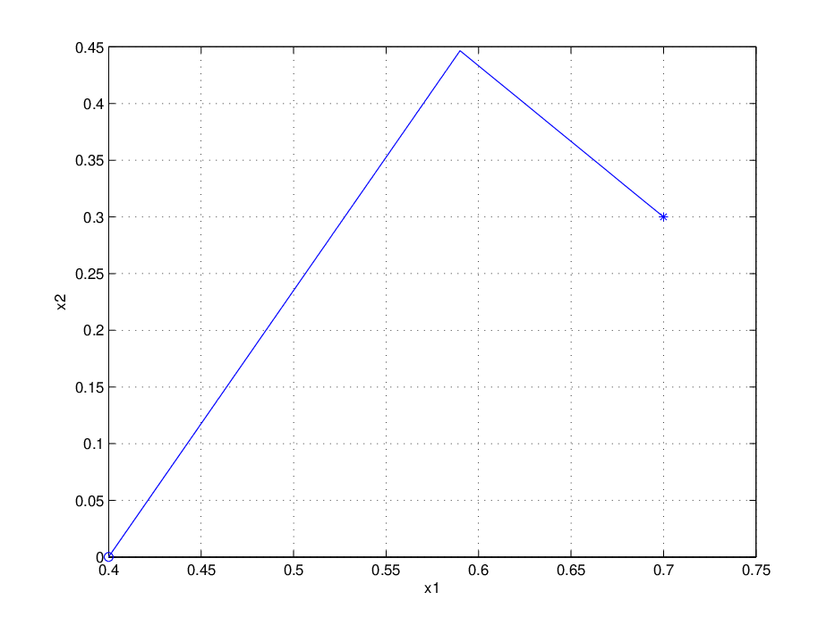
Figure 7 illustrates that, when θ1+h1<k1γ1<θ1max\theta_{1}+h_{1}<\frac{k_{1}}{\gamma_{1}}<\theta_{1}^{\max}, 0<k2γ2<θ2+h20<\frac{k_{2}}{\gamma_{2}}<\theta_{2}+h_{2}, the solution converges to z1∗=[k1γ1,k2γ2,1,0]⊤z^{*}_{1}=[\frac{k_{1}}{\gamma_{1}},\frac{k_{2}}{\gamma_{2}},1,0]^{\top}. Initially, the concentration of protein A (x1)(x_{1}) is low, which inhibits the expression of gene ​b{\emph{b}}, hence the concentration of protein B (x2)(x_{2}) decreases and activates the expression of gene a. However, after finite time, while the concentration of protein A is above the level θ1+h1\theta_{1}+h_{1}, which can permit the expression of gene b, the concentration of protein B increases. Finally, the concentrations of protein A and B come to the equilibrium (k1γ1,k2γ2).(\frac{k_{1}}{\gamma_{1}},\frac{k_{2}}{\gamma_{2}}). This confirms the result in Proposition 3.5.
Refer to caption
(a) xx components.
Refer to caption
(b) qq components.
Figure 7: The xx and qq components of a solution to ℋ\cal H in (8) converging to z1∗.z^{*}_{1}. The initial condition is given by q1​(0,0)=0q_{1}(0,0)=0, q2​(0,0)=0q_{2}(0,0)=0, x1​(0,0)=0.4x_{1}(0,0)=0.4, x2​(0,0)=0.4x_{2}(0,0)=0.4. The parameters are as follows: θ1=0.6\theta_{1}=0.6, θ2=0.5\theta_{2}=0.5, k1=0.7k_{1}=0.7, k2=0.4k_{2}=0.4, γ1=1\gamma_{1}=1, γ2=1\gamma_{2}=1, h1=0.01h_{1}=0.01, h2=0.01h_{2}=0.01. The symbol ∗* denotes the initial point and ∘\circ the point that the solution converges to (i.e., z1∗z^{*}_{1}).

4.1.2 Case 2 of Table 1

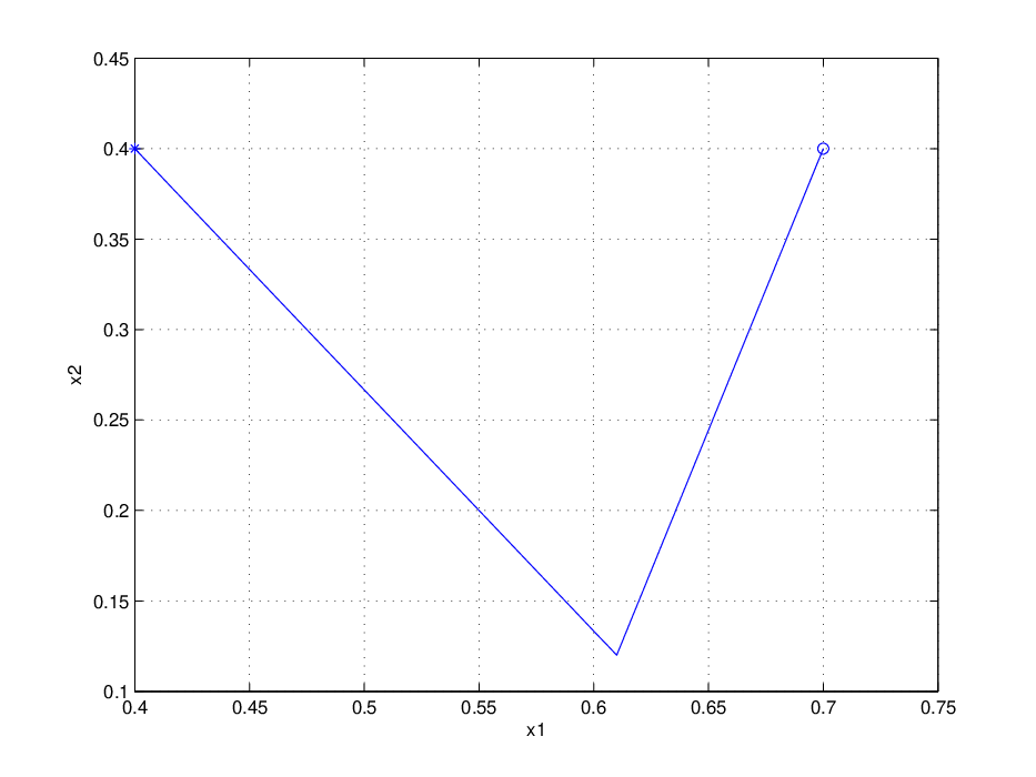
Figure 8 shows a solution to the equilibrium point z2∗=[k1γ1,0,0,0]⊤z^{*}_{2}=[\frac{k_{1}}{\gamma_{1}},0,0,0]^{\top} with 0<k1γ1<θ1−h10<\frac{k_{1}}{\gamma_{1}}<\theta_{1}-h_{1}. While both gene a and gene b are expressed at rate kik_{i}, for gene a, its degradation is faster than synthesis. When the concentration of protein A (x1)(x_{1}) is below some level, gene b is inhibited. This confirms the result in Proposition  3.5.

Refer to caption
(a) xx components.
Refer to caption
(b) qq components.
Figure 8: The xx and qq components of a solution to ℋ\cal H in (8) converging to z2∗.z^{*}_{2}. The initial condition is given by q1​(0,0)=1q_{1}(0,0)=1, q2​(0,0)=0q_{2}(0,0)=0, x1​(0,0)=0.7x_{1}(0,0)=0.7, x2​(0,0)=0.3x_{2}(0,0)=0.3. The parameters are as follows: θ1=0.6\theta_{1}=0.6, θ2=0.5\theta_{2}=0.5, k1=0.4k_{1}=0.4, k2=0.7k_{2}=0.7, γ1=1\gamma_{1}=1, γ2=1\gamma_{2}=1, h1=0.01h_{1}=0.01, h1=0.01h_{1}=0.01. The symbol ∗* denotes the initial point and ∘\circ is the point that the solution converges to (i.e., z2∗z_{2}^{*}).

4.1.3 Case 3 of Table 1

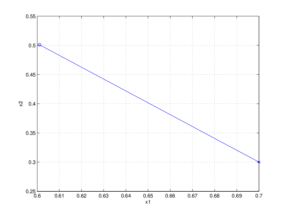
Figure 9 indicates that, when θ1−h1<k1γ1<θ1+h1\theta_{1}-h_{1}<\frac{k_{1}}{\gamma_{1}}<\theta_{1}+h_{1}, 0<k2γ2<θ2+h20<\frac{k_{2}}{\gamma_{2}}<\theta_{2}+h_{2} with the initial value z⁡(0,0)∈C2:={q1=1,q2=0,x1≥θ1−h1,x2≤θ2+h2}z(0,0)\in C_{2}:=\{q_{1}=1,q_{2}=0,x_{1}\geq\theta_{1}-h_{1},x_{2}\leq\theta_{2}+h_{2}\}. The solution flows towards z1∗=[k1γ1,k2γ2,1,0]⊤z^{*}_{1}=[\frac{k_{1}}{\gamma_{1}},\frac{k_{2}}{\gamma_{2}},1,0]^{\top}. Under these conditions, gene a and gene b are expressed at rate kik_{i}, i=1,2i=1,2, respectively. However, for gene a, its degradation is faster than its synthesis. This confirms the result in Proposition 3.6.
Refer to caption
(a) xx components.
Refer to caption
(b) qq components.
Figure 9: The xx and qq components of a solution to ℋ\cal H in (8) converging to z1∗.z^{*}_{1}. The initial conditions are given by q1​(0,0)=1q_{1}(0,0)=1, q2​(0,0)=0q_{2}(0,0)=0, x1​(0,0)=0.7x_{1}(0,0)=0.7, x2​(0,0)=0.3x_{2}(0,0)=0.3. The parameters are as follows: θ1=0.6\theta_{1}=0.6, θ2=0.5\theta_{2}=0.5, k1=0.601k_{1}=0.601, k2=0.501k_{2}=0.501, γ1=1\gamma_{1}=1, γ2=1\gamma_{2}=1, h1=0.02h_{1}=0.02, h1=0.02h_{1}=0.02. The symbol ∗* denotes the initial point and ∘\circ is the point that the solution converges to (i.e., z1∗z_{1}^{*}).
Refer to caption
(a) xx components.
Refer to caption
(b) qq components.
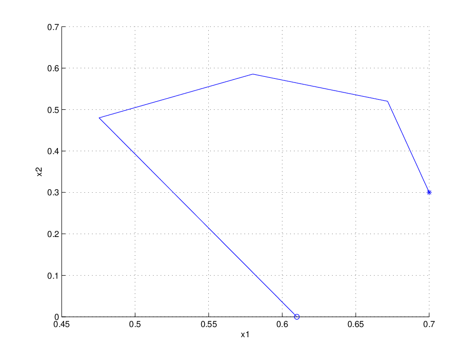
Figure 10: The xx and qq components of a solution to ℋ\cal H in (8) converging to z1∗.z^{*}_{1}. The initial conditions are given by q1​(0,0)=1q_{1}(0,0)=1, q2​(0,0)=1q_{2}(0,0)=1, x1​(0,0)=0.7x_{1}(0,0)=0.7, x2​(0,0)=0.7x_{2}(0,0)=0.7. The parameters are as follows: θ1=0.6\theta_{1}=0.6, θ2=0.5\theta_{2}=0.5, k1=0.601k_{1}=0.601, k2=0.501k_{2}=0.501, γ1=1\gamma_{1}=1, γ2=1\gamma_{2}=1, h1=0.02h_{1}=0.02, h1=0.02h_{1}=0.02. The symbol ∗* is the initial point and ∘\circ is the point that the solution converges to (i.e., z2∗z_{2}^{*}).

Figure 10 illustrates the case when θ1−h1≤k1γ1≤θ1+h1\theta_{1}-h_{1}\leq\frac{k_{1}}{\gamma_{1}}\leq\theta_{1}+h_{1}, k2γ2≤θ2+h2.\frac{k_{2}}{\gamma_{2}}\leq\theta_{2}+h_{2}. With the initial value z⁡(0,0)∉C2z(0,0)\notin C_{2}, the solution converges to z2∗=[k1γ1,0,0,0]⊤z^{*}_{2}=[\frac{k_{1}}{\gamma_{1}},0,0,0]^{\top}. With these conditions, initially, gene b is expressed at k2k_{2} and gene a is inhibited. After finite time, as the concentration of protein A (x1)(x_{1}) is lower than θ1−h1\theta_{1}-h_{1}, gene b becomes inhibited. Gene a is expressed at k1k_{1} while the concentration of protein B (x2)(x_{2}) is below a certain level. This confirms the result in Proposition 3.6.

4.1.4 Case 4 of Table 1

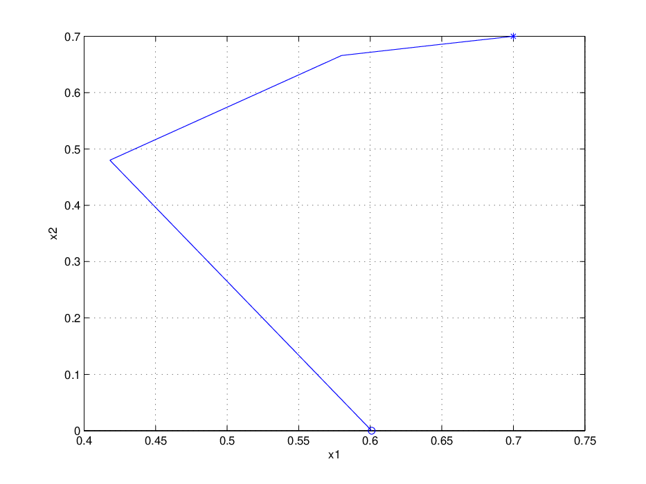
Figure 11 indicates that, when θ1−h1<k1γ1<θ1+h1\theta_{1}-h_{1}<\frac{k_{1}}{\gamma_{1}}<\theta_{1}+h_{1}, θ2+h2<k2γ2<θ2m​a​x\theta_{2}+h_{2}<\frac{k_{2}}{\gamma_{2}}<\theta_{2}^{max} with the initial value z⁡(0,0)∈C2:={q1=1,q2=0,x1≥θ1−h1,x2≤θ2+h2}z(0,0)\in C_{2}:=\{q_{1}=1,q_{2}=0,x_{1}\geq\theta_{1}-h_{1},x_{2}\leq\theta_{2}+h_{2}\}. The solution flows towards z2∗=[k1γ1,0,0,0]⊤z^{*}_{2}=[\frac{k_{1}}{\gamma_{1}},0,0,0]^{\top}. Under these conditions, gene a and gene b are expressed at rate kik_{i}, i=1,2i=1,2 initially. After some time, the concentration of protein B exceeds a centain level, which triggers a jump, after which the expression of gene a is inhibited. When the concentraion of protein A decreases enough, another jump occurs, after which the expression of gene b is inhibited as well. Eventually, the concentration of protein B reaches a low enough value to trigger another jump, after which the expression of gene a is activated, and the concentrations approach a steady-state value. This simulation confirms the result in Proposition 3.6.
Refer to caption
(a) xx components.
Refer to caption
(b) qq components.
Figure 11: The xx and qq components of a solution to ℋ\cal H in (8) converging to z2∗.z^{*}_{2}. The initial conditions are given by q1​(0,0)=1q_{1}(0,0)=1, q2​(0,0)=0q_{2}(0,0)=0, x1​(0,0)=0.7x_{1}(0,0)=0.7, x2​(0,0)=0.3x_{2}(0,0)=0.3. The parameters are as follows: θ1=0.6\theta_{1}=0.6, θ2=0.5\theta_{2}=0.5, k1=0.61k_{1}=0.61, k2=1k_{2}=1, γ1=1\gamma_{1}=1, γ2=1\gamma_{2}=1, h1=0.02h_{1}=0.02, h1=0.02h_{1}=0.02. The symbol ∗* denotes the initial point and ∘\circ is the point that the solution converges to (i.e., z2∗z_{2}^{*}).

4.2 Equilibrium set SS

When the parameters are in the region θ1+h1<k1γ1<θ1max,θ2+h2<k2γ2<θ2max\theta_{1}+h_{1}<\frac{k_{1}}{\gamma_{1}}<\theta_{1}^{\max},\theta_{2}+h_{2}<\frac{k_{2}}{\gamma_{2}}<\theta_{2}^{\max}, the set of points SS in (9) defines the equilibria. First, we compute this set of points for particular values of k1,k2,h1,h2,γ1=γ2=γ,θ1,θ2.k_{1},k_{2},h_{1},h_{2},\gamma_{1}=\gamma_{2}=\gamma,\theta_{1},\theta_{2}. Let k1=1k_{1}=1, k2=1k_{2}=1, γ1=γ2=γ=1\gamma_{1}=\gamma_{2}=\gamma=1, θ1=0.6\theta_{1}=0.6, θ2=0.5\theta_{2}=0.5, h1=0.01h_{1}=0.01, h2=0.01h_{2}=0.01. Then, using Corollary 3.4, the point p0p_{0} is given by p0​(1)=0.4966p_{0}(1)=0.4966. Then, from (3.3)-(3.3), we obtain p0=[0.49660.49],p1=[0.610.3796],p2=[0.6920.51],p3=[0.590.5822].p_{0}=\left[\begin{array}[]{c}0.4966\\ 0.49\end{array}\right],\ p_{1}=\left[\begin{array}[]{c}0.61\\ 0.3796\end{array}\right],\ p_{2}=\left[\begin{array}[]{c}0.692\\ 0.51\end{array}\right],\ p_{3}=\left[\begin{array}[]{c}0.59\\ 0.5822\end{array}\right]. With the values of p0,p1,p2,p3p_{0},p_{1},p_{2},p_{3}, the set SS in (9) is given by

S1\displaystyle S_{1} =\displaystyle= {x:x2=−0.973381x1+0.973381,\displaystyle\{x:x_{2}=-0.973381x_{1}+0.973381,
0.4966≤x1≤0.61,0.3796≤x2≤0.49}×{(0,0)},\displaystyle\hskip 14.45377pt0.4966\leq x_{1}\leq 0.61,0.3796\leq x_{2}\leq 0.49\}\times\{(0,0)\},
S2\displaystyle S_{2} =\displaystyle= {x:x2=1.590722x1−0.590722,\displaystyle\{x:x_{2}=1.590722x_{1}-0.590722,
0.61≤x1≤0.692,0.3796≤x2≤0.51}×{(1,0)},\displaystyle\hskip 14.45377pt0.61\leq x_{1}\leq 0.692,0.3796\leq x_{2}\leq 0.51\}\times\{(1,0)\},
S3\displaystyle S_{3} =\displaystyle= {x:x2=−0.7081296x1+1,\displaystyle\{x:x_{2}=-0.7081296x_{1}+1,
0.59≤x1≤0.692,0.51≤x2≤0.5822}×{(1,1)},\displaystyle\hskip 14.45377pt0.59\leq x_{1}\leq 0.692,0.51\leq x_{2}\leq 0.5822\}\times\{(1,1)\},
S4\displaystyle S_{4} =\displaystyle= {x:x2=0.9871896x1−0.000238,\displaystyle\{x:x_{2}=0.9871896x_{1}-0.000238,
0.4966≤x1≤0.59,0.49≤x2≤0.5822}×{(0,1)}.\displaystyle\hskip 14.45377pt0.4966\leq x_{1}\leq 0.59,0.49\leq x_{2}\leq 0.5822\}\times\{(0,1)\}.
Refer to caption
(a) SS
Refer to caption
(b) x1x_{1} component
Figure 12: Set SS for parameters k1=1k_{1}=1, k2=1k_{2}=1, γ1=1\gamma_{1}=1, γ2=1\gamma_{2}=1, θ1=0.6\theta_{1}=0.6, θ2=0.5\theta_{2}=0.5, h1=0.01h_{1}=0.01, h2=0.01.h_{2}=0.01.

Figure 12(a) shows the set of points SS projected to ℝ2\mathbb{R}^{2} for these parameters. For the same parameter values, the period of the limit cycle obtained from Corollary 3.4 is T=0.8230​ sec,T=0.8230\mbox{ sec}, where t1′=0.2552​ sect_{1}^{\prime}=0.2552\mbox{ sec}, t2′=0.2359​ sect_{2}^{\prime}=0.2359\mbox{ sec}, t3′=0.1594​ sect_{3}^{\prime}=0.1594\mbox{ sec}, t4′=0.1724​ sec.t_{4}^{\prime}=0.1724\mbox{ sec}. Figure 12(b) confirms this result.

Refer to caption
(a) h1=0.015h_{1}=0.015, h2=0.015h_{2}=0.015
Refer to caption
(b) h1=0.01h_{1}=0.01, h2=0.01h_{2}=0.01
Refer to caption
(c) h1=0.006h_{1}=0.006, h2=0.006h_{2}=0.006
Refer to caption
(d) h1=0h_{1}=0, h2=0h_{2}=0
Figure 13: Solutions approaching the set SS with different initial conditions of zz and fixed parameters θ1=0.6\theta_{1}=0.6, θ2=0.5\theta_{2}=0.5, γ1=1\gamma_{1}=1, γ2=1\gamma_{2}=1, k1=1k_{1}=1, k2=1k_{2}=1.

Figure 13 shows simulations with several initial conditions and common parameters θ1=0.6,θ2=0.5,γ1=1,γ2=1,k1=1,k2=1\theta_{1}=0.6,\theta_{2}=0.5,\gamma_{1}=1,\gamma_{2}=1,k_{1}=1,k_{2}=1, but decreasing h1,h2h_{1},h_{2}. Each solution converges to the limit cycle SS. The size of the limit cycle is reduced as h1,h2h_{1},h_{2} gets smaller. From our results we know that the size of the limit cycle depends on the value of hysteresis parameters. When the magnitude of hysteresis tends to zero, the set SS approaches a point, which is given by (θ1\theta_{1}, θ2\theta_{2}) (see similar case shown in Figure 13(d).)

Figure 14 shows simulations with several initial conditions and common parameters θ1=0.6,θ2=0.5,γ1=1,γ2=1,h1=0.01,h2=0.01\theta_{1}=0.6,\theta_{2}=0.5,\gamma_{1}=1,\gamma_{2}=1,h_{1}=0.01,h_{2}=0.01, but changing k1,k2k_{1},k_{2}. Each solution converges to the limit cycle SS (in cyan). The blue set of points defines the limit cycle SS generated when k1=k2=1.k_{1}=k_{2}=1. The variations of k1k_{1} and k2k_{2} can be considered to be perturbations as in Theorem 3.8. The simulations show that the smaller the perturbation on these constants, the closer the limit cycle becomes to the nominal one. Figure 15 shows simulations with several initial conditions and common parameters θ1=0.6,θ2=0.5,k1=1,k2=1,h1=0.01,h2=0.01\theta_{1}=0.6,\theta_{2}=0.5,k_{1}=1,k_{2}=1,h_{1}=0.01,h_{2}=0.01, but now with γ1\gamma_{1} and γ2\gamma_{2} varying.

Refer to caption
(a) k1=0.8k_{1}=0.8, k2=0.8k_{2}=0.8
Refer to caption
(b) k1=0.9k_{1}=0.9, k2=0.9k_{2}=0.9
Refer to caption
(c) k1=1.1k_{1}=1.1, k2=1.1k_{2}=1.1
Refer to caption
(d) k1=1.2k_{1}=1.2, k2=1.2k_{2}=1.2
Figure 14: Solutions approaching the set SS with different initial conditions of zz and fixed parameters θ1=0.6\theta_{1}=0.6, θ2=0.5\theta_{2}=0.5, γ1=1\gamma_{1}=1, γ2=1\gamma_{2}=1, h1=0.01h_{1}=0.01, h2=0.01h_{2}=0.01.
Refer to caption
(a) k1=0.8k_{1}=0.8, k2=0.8k_{2}=0.8
Refer to caption
(b) γ1=0.9\gamma_{1}=0.9, γ2=0.9\gamma_{2}=0.9
Refer to caption
(c) γ1=1.1\gamma_{1}=1.1, γ2=1.1\gamma_{2}=1.1
Refer to caption
(d) γ1=1.2\gamma_{1}=1.2, γ2=1.2\gamma_{2}=1.2
Figure 15: Solutions approaching the set SS with different initial conditions of zz and fixed parameters θ1=0.6\theta_{1}=0.6, θ2=0.5\theta_{2}=0.5, k1=1k_{1}=1, k2=1k_{2}=1, h1=0.01h_{1}=0.01, h2=0.01h_{2}=0.01.

Finally, Figure 16 shows the case when γ1≠γ2\gamma_{1}\neq\gamma_{2}. In this case, the trajectories approach the limit cycle given in (9).

Refer to caption
Figure 16: Solutions approaching the set SS with different initial conditions of xix_{i} and fixed parameters. Values of parameters: θ1=0.6,θ2=0.5,γ1=5,γ2=1,k1=5,k2=1,h1=0.01,h1=0.01\theta_{1}=0.6,\theta_{2}=0.5,\gamma_{1}=5,\gamma_{2}=1,k_{1}=5,k_{2}=1,h_{1}=0.01,h_{1}=0.01. The blue line is the set SS. The symbol ∗* denotes the initial point.

5 Conclusion

In this paper, a mathematical model of a genetic regulatory network has been developed under the formalism of hybrid dynamical systems. The model presented in this paper permits a quantitative analysis of the cellular protein dynamics under the influence of protein concentration thresholds and initial conditions. The analysis of the hybrid model with two genes determines conditions guaranteeing the existence of solutions, the equilibria of the system, stability properties of the equilibria and its robustness. In particular, we have revealed conditions on the parameters that, when hysteresis is present, the interaction between the concentrations of two proteins leads to oscillatory behavior. Such a behavior is impossible in a two-gene network without hysteresis. The obtained results are an important initial step in the analysis of genetic regulatory networks using hybrid systems theory, which we believe has great potential for the understanding of the complex mechanisms in such networks, in particular, when treated as (larger than two) interconnections of hybrid systems.

References

  • [1] H. de Jong, Modeling and simulation of genetic regulatory systems: a literature review, Journal of Computational Biology 9 (1) (2002) 67–103.
  • [2] M. Chaves, E. D. Sontag, R. Albert, Methods of robustness analysis for boolean models of gene control networks, Journal of Theoretical Biology 235 (2005) 431–449.
  • [3] L. Glass, L. Kauffman, The logical analysis of continuous, non-linear biochemical control networks, J. Theor. Biol. 39 (1) (1973) 103–129.
  • [4] E. H. Snoussi, Qualitative dynamics of piecewise-linear differential equations: a discrete mapping approach, Dynamics and Stability of Systems 4 (3–4) (1989) 565–583.
  • [5] J. L. Gouze´\acute{e}, T. Sari, A class of piecewise linear differential equations arising in biological models, Dynam. Syst. 17 (4) (2002) 299–316.
  • [6] H. de Jong, J. L. Gouze´\acute{e}, C. Hernandez, M. Page, T. Sari, J. Geiselmann, Hybrid modeling and simulation of genetic regulatory networks: A qualitative approach, Hybrid Systems: Computation and Control (2003) 267–282.
  • [7] P. Lincoln, A. Tiwari, Symbolic systems biology: Hybrid modeling and analysis of biological networks, Hybrid Systems: Computation and Control 2293 (2004) 660–672.
  • [8] R. Ghosh, C. J. Tomlin, Lateral inhibition through delta-notch signaling: A piecewise-affine hybrid model, Hybrid Systems: Computation and Control 2034 (2001) 232–246.
  • [9] V. Noel, D. Grigoriev, S. Vakulenko, O. Radulescu, Hybrid models of the cell cycle molecular machinery, First International Workshop on Hybrid Systems and Biology 23 (2012) 88–105.
  • [10] S. Huang, Gene expression profiling, genetic networks, and cellular states: an integrating concept for tumorigenesis and drug discovery, Journal of Molecular Medicine 77 (1999) 469–480.
  • [11] J. Das, M. Ho, J. Zikherman, C. Govern, M. Yang, A. Weiss, A. K. Chakraborty, J. P. Roose, Digital signaling and hysteresis characterize ras activation in lymphoid cells, Cells 136 (2009) 337–351.
  • [12] B. P. Kramer, M. Fussenegger, Hysteresis in a synthetic mammalian gene network, Proceedings of the National Academy of Sciences (USA) 102 (2005) 9517–9522.
  • [13] J. Hu, K. R. Qin, C. Xiang, T. H. Lee, Modeling of hysteresis in a mammalian gene regulatory network, 9th Annual International Conference on Computational Systems Bioinformatics 9 (2010) 50–55.
  • [14] L. Qiao, R. B. Nachbar, I. G, Bistability and oscillations in the huang-ferrell model of mapk signalling, PLoS Computational Biology 3 (9) (2007) 1819–1826.
  • [15] A. Kuznetsov, M. Kaern, N. Kopell, Synchrony in a population of hysteresis-based genetic oscillators, SIAM Journal of Applied Mathematics 65 (2) (2004) 392–425.
  • [16] Z. Han, L. Yang, W. R. Maclellan, J. N. Weiss, Z. Qu, Hysteresis and cell cycle transitions: How crucial is it?, Biophysical Journal 88 (2005) 1626–1634.
  • [17] J. Kim, T. G. Kim, S. H. Jung, J. R. Kim, T. Park, P. H. Harrison, K. H. Cho, Evolutionary design principles of modules that control cellular differentiation: consequences for hysteresis and multistationarity, Bioinformatics 24 (13) (2008) 1516–1522.
  • [18] R. Goebel, R. G. Sanfelice, A. R. Teel, Hybrid dynamical systems, IEEE Control Systems Magazine (2009) 28–93.
  • [19] T. Mestl, E. Plahte, S. W. Omholt, A mathematical framework for describing and analysing gene regulatory networks, Journal of Theoretical Biology 176 (1995) 291–300.
  • [20] R. Goebel, R. G. Sanfelice, A. R. Teel, Hybrid Dynamical Systems: Modeling, Stability, and Robustness, Princeton University Press, 2012.
  • [21] R. G. Sanfelice, R. Goebel, A. R. Teel, Invariance principles for hybrid systems with connections to detectability and asymptotic stability, IEEE Transactions on Automatic Control 52 (12) (2007) 2282–2297.
  • [22] R. G. Sanfelice, D. A. Copp, P. Nanez, A toolbox for simulation of hybrid systems in Matlab/Simulink: Hybrid Equations (HyEQ) Toolbox, 2013, pp. 101–106.

Appendix A

A.1 Proof of Proposition 3.3

We consider the first three cases in Table 1. Since for every point in DD, the jump map GG changes the value of at least one of the logic variables, we just need to consider the case when z∗∈Cz^{*}\in C to determine isolated equilibrium points z∗z^{*}. The continuous state xx of the system satisfies

x˙=[k1​(1−q2)−γ1​x1k2​q1−γ2​x2].\dot{x}=\left[\begin{array}[]{cc}k_{1}(1-q_{2})-\gamma_{1}x_{1}\\ k_{2}q_{1}-\gamma_{2}x_{2}\\ \end{array}\right].

To compute equilibrium points, let F⁡(z∗)=0F(z^{*})=0. Then,

[k1​(1−q2∗)−γ1​x1∗k2​q1∗−γ2​x2∗]=0\left[\begin{array}[]{ll}k_{1}(1-q_{2}^{*})-\gamma_{1}x_{1}^{*}\\ k_{2}q_{1}^{*}-\gamma_{2}x_{2}^{*}\\ \end{array}\right]=0

and solving for x∗x^{*} leads to

x∗=[k1​(1−q2∗)γ1k2​q1∗γ2].x^{*}=\left[\begin{array}[]{cc}\frac{k_{1}(1-q_{2}^{*})}{\gamma_{1}}\\ \frac{k_{2}q_{1}^{*}}{\gamma_{2}}\end{array}\right].

According to the possible values of q∗q^{*}, all the possibilities of x∗x^{*} are listed in Table 2. These define vectors za∗z_{a}^{*}, zb∗z_{b}^{*}, zc∗z_{c}^{*}, and zd∗z_{d}^{*}, which are to be checked if they satisfy z∗∈Cz^{*}\in C.

Table 2: Values of x∗x^{*} based on different combinations of the values of q∗q^{*}.
x∗x^{*} q∗q^{*}
za∗z_{a}^{*} (k1γ1,k2γ2)(\frac{k_{1}}{\gamma_{1}},\frac{k_{2}}{\gamma_{2}}) q1∗=1q_{1}^{*}=1, q2∗=0q_{2}^{*}=0
zb∗z_{b}^{*} (0,0)(0,0) q1∗=0q_{1}^{*}=0, q2∗=1q_{2}^{*}=1
zc∗z_{c}^{*} (0,k2γ2)(0,\frac{k_{2}}{\gamma_{2}}) q1∗=1q_{1}^{*}=1, q2∗=1q_{2}^{*}=1
zd∗z_{d}^{*} (k1γ1,0)(\frac{k_{1}}{\gamma_{1}},0) q1∗=0q_{1}^{*}=0, q2∗=0q_{2}^{*}=0

Similar to CC, the jump set DD can also be written as D=⋃i=14DiD=\bigcup^{4}_{i=1}D_{i}, where D1:={z∈𝒵:q1=0,q2=0,x1=θ1+h1,x2≤θ2+h2}∪{z∈𝒵:q1=1,q2=0,x1=θ1−h1,x2≤θ2+h2}D_{1}:=\{z\in{\cal{Z}}:q_{1}=0,q_{2}=0,x_{1}=\theta_{1}+h_{1},x_{2}\leq\theta_{2}+h_{2}\}\cup\{z\in{\cal{Z}}:q_{1}=1,q_{2}=0,x_{1}=\theta_{1}-h_{1},x_{2}\leq\theta_{2}+h_{2}\}, D2:={z∈𝒵:q1=1,q2=1,x1=θ1−h1,x2≥θ2−h2}∪{z∈𝒵:q1=0,q2=1,x1=θ1+h1,x2≥θ2−h2}D_{2}:=\{z\in{\cal{Z}}:q_{1}=1,q_{2}=1,x_{1}=\theta_{1}-h_{1},x_{2}\geq\theta_{2}-h_{2}\}\cup\{z\in{\cal{Z}}:q_{1}=0,q_{2}=1,x_{1}=\theta_{1}+h_{1},x_{2}\geq\theta_{2}-h_{2}\}, D3:={z∈𝒵:q1=1,q2=0,x1≥θ1−h1,x2=θ2+h2}∪{z∈𝒵:q1=1,q2=1,x1≥θ1−h1,x2=θ2−h2}D_{3}:=\{z\in{\cal{Z}}:q_{1}=1,q_{2}=0,x_{1}\geq\theta_{1}-h_{1},x_{2}=\theta_{2}+h_{2}\}\cup\{z\in{\cal{Z}}:q_{1}=1,q_{2}=1,x_{1}\geq\theta_{1}-h_{1},x_{2}=\theta_{2}-h_{2}\}, D4:={z∈𝒵:q1=0,q2=1,x1≤θ1+h1,x2=θ2−h2}∪{z∈𝒵:q1=0,q2=0,x1≤θ1+h1,x2=θ2+h2}D_{4}:=\{z\in{\cal{Z}}:q_{1}=0,q_{2}=1,x_{1}\leq\theta_{1}+h_{1},x_{2}=\theta_{2}-h_{2}\}\cup\{z\in{\cal{Z}}:q_{1}=0,q_{2}=0,x_{1}\leq\theta_{1}+h_{1},x_{2}=\theta_{2}+h_{2}\}. Now, we find the value of x1∗,x2∗x_{1}^{*},x_{2}^{*}, q1∗,q2∗q_{1}^{*},q_{2}^{*} such that z∗∈C.z^{*}\in C.

  • •

    Case ii: Consider parameters such that θ1+h1<k1γ1<θ1max\theta_{1}+h_{1}<\frac{k_{1}}{\gamma_{1}}<\theta_{1}^{\max}, 0<k2γ2<θ2+h2.0<\frac{k_{2}}{\gamma_{2}}<\theta_{2}+h_{2}. Then, it can be checked that

    za∗∈C,zb∗∉C,zc∗∉C,zd∗∉C.z_{a}^{*}\in C,z_{b}^{*}\notin C,z_{c}^{*}\notin C,z_{d}^{*}\notin C.

    Then, za∗z^{*}_{a} is an equilibrium point.

  • •

    Case i​iii: Consider parameters such that 0<k1γ1<θ1−h10<\frac{k_{1}}{\gamma_{1}}<\theta_{1}-h_{1}, 0<k2γ2<θ2+h2.0<\frac{k_{2}}{\gamma_{2}}<\theta_{2}+h_{2}. Then, it can be checked that

    za∗∉C,zb∗∉C,zc∗∉C,zd∗∈C.z_{a}^{*}\notin C,z_{b}^{*}\notin C,z_{c}^{*}\notin C,z_{d}^{*}\in C.

    Then, zd∗z_{d}^{*} is an equilibrium point.

  • •

    Case i​i​iiii: Consider parameters such that θ1+h1<k1γ1<θ1max\theta_{1}+h_{1}<\frac{k_{1}}{\gamma_{1}}<\theta_{1}^{\max}, θ2+h2<k2γ2<θ2max.\theta_{2}+h_{2}<\frac{k_{2}}{\gamma_{2}}<\theta_{2}^{\max}. Then, it can be checked that

    za∗∉C,zb∗∉C,zc∗∉C,zd∗∉C.z_{a}^{*}\notin C,z_{b}^{*}\notin C,z_{c}^{*}\notin C,z_{d}^{*}\notin C.
  • •

    Case i​viv: Consider parameters such that 0<k1γ1<θ1−h10<\frac{k_{1}}{\gamma_{1}}<\theta_{1}-h_{1}, θ2+h2<k2γ2<θ2max.\theta_{2}+h_{2}<\frac{k_{2}}{\gamma_{2}}<\theta_{2}^{\max}. Then, it can be checked that

    za∗∉C,zb∗∉C,zc∗∉C,zd∗∈C.z_{a}^{*}\notin C,z_{b}^{*}\notin C,z_{c}^{*}\notin C,z_{d}^{*}\in C.

    Then, zd∗z_{d}^{*} is an equilibrium point.

  • •

    Case vv: Consider parameters such that θ1−h1<k1γ1<θ1+h1\theta_{1}-h_{1}<\frac{k_{1}}{\gamma_{1}}<\theta_{1}+h_{1}, 0<k2γ2<θ2+h2.0<\frac{k_{2}}{\gamma_{2}}<\theta_{2}+h_{2}. Then, it can be checked that

    za∗∈C,zb∗∉C,zc∗∉C,zd∗∈Cz_{a}^{*}\in C,z_{b}^{*}\notin C,z_{c}^{*}\notin C,z_{d}^{*}\in C

    Then, za∗z_{a}^{*} and zd∗z_{d}^{*} are equilibrium points.

  • •

    Case v​ivi: Consider parameters such that θ1−h1<k1γ1<θ1+h1\theta_{1}-h_{1}<\frac{k_{1}}{\gamma_{1}}<\theta_{1}+h_{1}, θ2+h2<k2γ2<θ2m​a​x.\theta_{2}+h_{2}<\frac{k_{2}}{\gamma_{2}}<\theta_{2}^{max}. Then, it can be checked that

    za∗∉C,zb∗∉C,zc∗∉C,zd∗∈Cz_{a}^{*}\notin C,z_{b}^{*}\notin C,z_{c}^{*}\notin C,z_{d}^{*}\in C

    Then, zd∗z_{d}^{*} is an equilibrium point.

From the properties above, only za∗z_{a}^{*} and zd∗z_{d}^{*} are candidate isolate equilibrium points. We show that the first four cases in Table 1 are equilibrium points of the entire system with z1∗=za∗z_{1}^{*}=z_{a}^{*} and z2∗=zd∗z_{2}^{*}=z_{d}^{*}. For case 1, which is when θ1+h1<k1γ1<θ1max,0<k2γ2<θ2+h2\theta_{1}+h_{1}<\frac{k_{1}}{\gamma_{1}}<\theta_{1}^{\max},0<\frac{k_{2}}{\gamma_{2}}<\theta_{2}+h_{2}, we pick any other z′≠z1∗z^{\prime}\neq z_{1}^{*}. We have that if z′∈Cz^{\prime}\in C then F⁡(z′)≠0F(z^{\prime})\neq 0, so z1∗z_{1}^{*} is the isolated equilibrium point of the system. For case 2, when 0<k1γ1<θ1−h10<\frac{k_{1}}{\gamma_{1}}<\theta_{1}-h_{1}, we pick any other z′≠z2∗z^{\prime}\neq z^{*}_{2}. If z′∈Cz^{\prime}\in C, then F⁡(z′)≠0F(z^{\prime})\neq 0, so z2∗z^{*}_{2} is the isolated equilibrium point of the system. For case 3, when θ1−h1<k1γ1<θ1+h1\theta_{1}-h_{1}<\frac{k_{1}}{\gamma_{1}}<\theta_{1}+h_{1}, 0<k2γ2<θ2+h20<\frac{k_{2}}{\gamma_{2}}<\theta_{2}+h_{2}, we pick any other z′≠zi∗z^{\prime}\neq z^{*}_{i} for each i∈{1,2}i\in\{1,2\}. If z′∈Cz^{\prime}\in C, then F⁡(z′)≠0F(z^{\prime})\neq 0, so z1∗z^{*}_{1} or z2∗z^{*}_{2} are the equilibrium points of the entire system. For case 4, when θ1−h1<k1γ1<θ1+h1\theta_{1}-h_{1}<\frac{k_{1}}{\gamma_{1}}<\theta_{1}+h_{1}, θ2+h2<k2γ2<θ2m​a​x\theta_{2}+h_{2}<\frac{k_{2}}{\gamma_{2}}<\theta_{2}^{max} we pick any other z′≠z2∗z^{\prime}\neq z^{*}_{2}. If z′∈Cz^{\prime}\in C, then F⁡(z′)≠0F(z^{\prime})\neq 0, so z2∗z^{*}_{2} is the isolated equilibrium point of the system.

We now show that SS in (9) is an equilibrium set for case 5 of the parameters in Table 1, namely k1γ1∈(θ1+h1,θ1max)\frac{k_{1}}{\gamma_{1}}\in(\theta_{1}+h_{1},\theta_{1}^{\max}), k2γ2∈(θ2+h2,θ2max)\frac{k_{2}}{\gamma_{2}}\in(\theta_{2}+h_{2},\theta_{2}^{\max}). To this end, we establish that for parameters in such range, the logic variables evolve according to the state transition graph in Figure 18. This is due to the system not having an isolated equilibrium point in the flow set CC; see Case iii in the proof of Proposition 3.3. Let Q:={(0,0),(0,1),(1,0),(1,1)}Q:=\{(0,0),(0,1),(1,0),(1,1)\}. The xx component of the vector field FF satisfies the following properties on the boundary of CC.

Refer to caption
Figure 17: Vector fields on the boundaries of CC to case 5 of Table 1.
  1. 1.

    Points on the boundary of C1C_{1}:

    • •

      When x∈{x:x1=0,0≤x2≤θ2+h2},x\in\{x:x_{1}=0,0\leq x_{2}\leq\theta_{2}+h_{2}\}, the first two components of FF define the vector f1​(x):=[k1−γ2​x2]f_{1}(x):=\left[\begin{array}[]{cc}k_{1}\\ -\gamma_{2}x_{2}\end{array}\right]. Since k1>0k_{1}>0, γ2>0\gamma_{2}>0, then f1​(x)f_{1}(x) points inside of C1.C_{1}.

    • •

      When x∈{x:0≤x1≤θ1+h1,x2=0},x\in\{x:0\leq x_{1}\leq\theta_{1}+h_{1},x_{2}=0\}, f1​(x):=[k1−γ1​x10]f_{1}(x):=\left[\begin{array}[]{cc}k_{1}-\gamma_{1}x_{1}\\ 0\end{array}\right]. Since θ1+h1<k1γ1<θ1max\theta_{1}+h_{1}<\frac{k_{1}}{\gamma_{1}}<\theta^{\max}_{1}, then f1​(x)f_{1}(x) is tangent to the boundary of C1.C_{1}.

    • •

      When x∈{x:0≤x1≤θ1+h1,x2=θ2+h2},x\in\{x:0\leq x_{1}\leq\theta_{1}+h_{1},x_{2}=\theta_{2}+h_{2}\}, f1​(x):=[k1−γ1​x1−γ2​(θ2+h2)]f_{1}(x):=\left[\begin{array}[]{cc}k_{1}-\gamma_{1}x_{1}\\ -\gamma_{2}(\theta_{2}+h_{2})\end{array}\right]. Since θ1+h1<k1γ1<θmax\theta_{1}+h_{1}<\frac{k_{1}}{\gamma_{1}}<\theta^{\max},γ2>0\gamma_{2}>0, then f1​(x)f_{1}(x) points inside of C1.C_{1}.

    • •

      When x∈{x:x1=θ1+h1,0≤x2≤θ2+h2},x\in\{x:x_{1}=\theta_{1}+h_{1},0\leq x_{2}\leq\theta_{2}+h_{2}\}, f1​(x):=[k1−γ1​(θ1+h1)−γ2​x2]f_{1}(x):=\left[\begin{array}[]{cc}k_{1}-\gamma_{1}(\theta_{1}+h_{1})\\ -\gamma_{2}x_{2}\end{array}\right]. Since θ1+h1<k1γ1<θmax\theta_{1}+h_{1}<\frac{k_{1}}{\gamma_{1}}<\theta^{\max},γ2>0\gamma_{2}>0, then f1​(x)f_{1}(x) points outside of C1.C_{1}.

    Then, since there is no isolated equilibrium point in C1C_{1}, trajectories starting in C1C_{1} are such that the xx component flow towards {x1=θ1+h1,0≤x2≤θ2+h2}\{x_{1}=\theta_{1}+h_{1},0\leq x_{2}\leq\theta_{2}+h_{2}\}.

  2. 2.

    Points on the boundary of C2C_{2}:

    • •

      When x∈{x:x1=θ1−h1,0≤x2≤θ2+h2},x\in\{x:x_{1}=\theta_{1}-h_{1},0\leq x_{2}\leq\theta_{2}+h_{2}\}, f2​(x):=[k1−γ1​(θ1−h1)k2−γ2​x2]f_{2}(x):=\left[\begin{array}[]{cc}k_{1}-\gamma_{1}(\theta_{1}-h_{1})\\ k_{2}-\gamma_{2}x_{2}\end{array}\right]. Since θ1+h1<k1γ1<θ1max\theta_{1}+h_{1}<\frac{k_{1}}{\gamma_{1}}<\theta^{\max}_{1}, θ2+h2<k2γ2<θ2max\theta_{2}+h_{2}<\frac{k_{2}}{\gamma_{2}}<\theta^{\max}_{2}, then f2​(x)f_{2}(x) points inside of C2.C_{2}.

    • •

      When x∈{x:x1≥θ1−h1,x2=0},x\in\{x:x_{1}\geq\theta_{1}-h_{1},x_{2}=0\}, f2​(x):=[k1−γ1​x1k2]f_{2}(x):=\left[\begin{array}[]{cc}k_{1}-\gamma_{1}x_{1}\\ k_{2}\end{array}\right]. Since θ1+h1<k1γ1<θmax\theta_{1}+h_{1}<\frac{k_{1}}{\gamma_{1}}<\theta^{\max},θ2+h2<k2γ2<θ2max\theta_{2}+h_{2}<\frac{k_{2}}{\gamma_{2}}<\theta_{2}^{\max}, then f2​(x)f_{2}(x) points inside of C2.C_{2}.

    • •

      When x∈{x:x1≥θ1−h1,x2=θ2+h2},x\in\{x:x_{1}\geq\theta_{1}-h_{1},x_{2}=\theta_{2}+h_{2}\}, f2​(x):=[k1−γ1​x1k2−γ2​(θ2+h2)]f_{2}(x):=\left[\begin{array}[]{cc}k_{1}-\gamma_{1}x_{1}\\ k_{2}-\gamma_{2}(\theta_{2}+h_{2})\end{array}\right]. Since θ1+h1<k1γ1<θ1max\theta_{1}+h_{1}<\frac{k_{1}}{\gamma_{1}}<\theta^{\max}_{1}, θ2+h2<k2γ2<θ2max\theta_{2}+h_{2}<\frac{k_{2}}{\gamma_{2}}<\theta_{2}^{\max}, then f2​(x)f_{2}(x) points outside of C2.C_{2}.

    Then, since there is no isolated equilibrium point in C2C_{2}, trajectories starting in C2C_{2} are such that the xx component flow towards {x1≥θ1−h1,x2=θ2+h2}\{x_{1}\geq\theta_{1}-h_{1},x_{2}=\theta_{2}+h_{2}\}.

  3. 3.

    Points on the boundary of C3C_{3}:

    • •

      When x∈{x:x1≥θ1−h1,x2=θ2−h2},x\in\{x:x_{1}\geq\theta_{1}-h_{1},x_{2}=\theta_{2}-h_{2}\}, f3​(x):=[−γ1​x1k2−γ2​(θ2−h2)]f_{3}(x):=\left[\begin{array}[]{cc}-\gamma_{1}x_{1}\\ k_{2}-\gamma_{2}(\theta_{2}-h_{2})\end{array}\right]. Since θ1+h1<k1γ1<θ1max\theta_{1}+h_{1}<\frac{k_{1}}{\gamma_{1}}<\theta^{\max}_{1}, θ2+h2<k2γ2<θ2max\theta_{2}+h_{2}<\frac{k_{2}}{\gamma_{2}}<\theta_{2}^{\max}, then f3​(x)f_{3}(x) points inside of C3C_{3}.

    • •

      When x∈{x:x1=θ1−h1,x2≥θ2−h2},x\in\{x:x_{1}=\theta_{1}-h_{1},x_{2}\geq\theta_{2}-h_{2}\}, f3​(x):=[−γ1​(θ1−h1)k2−γ2​x2]f_{3}(x):=\left[\begin{array}[]{cc}-\gamma_{1}(\theta_{1}-h_{1})\\ k_{2}-\gamma_{2}x_{2}\end{array}\right]. Since θ1+h1<k1γ1<θ1max\theta_{1}+h_{1}<\frac{k_{1}}{\gamma_{1}}<\theta^{\max}_{1}, θ2+h2<k2γ2<θ2max\theta_{2}+h_{2}<\frac{k_{2}}{\gamma_{2}}<\theta_{2}^{\max}, then f3​(x)f_{3}(x) points outside of C3C_{3}.

    Then, since there is no isolated equilibrium point in C3C_{3}, the trajectories starting in C3C_{3} have xx component that flow towards {x1=θ1−h1,x2≥θ2−h2}\{x_{1}=\theta_{1}-h_{1},x_{2}\geq\theta_{2}-h_{2}\}.

  4. 4.

    Points on the boundary of C4C_{4}:

    • •

      When x∈{x:x1=θ1+h1,x2≥θ2−h2},x\in\{x:x_{1}=\theta_{1}+h_{1},x_{2}\geq\theta_{2}-h_{2}\}, f4​(x):=[−γ1​(θ1+h1)−γ2​x2]f_{4}(x):=\left[\begin{array}[]{cc}-\gamma_{1}(\theta_{1}+h_{1})\\ -\gamma_{2}x_{2}\end{array}\right]. Since γ1>0\gamma_{1}>0, γ2>0\gamma_{2}>0, then f4​(x)f_{4}(x) points inside of C4.C_{4}.

    • •

      When x∈{x:x1=0,x2≥θ2−h2},x\in\{x:x_{1}=0,x_{2}\geq\theta_{2}-h_{2}\}, f4​(x):=[0−γ2​x2]f_{4}(x):=\left[\begin{array}[]{cc}0\\ -\gamma_{2}x_{2}\end{array}\right]. Since γ2>0\gamma_{2}>0, then f4​(x)f_{4}(x) is tangent to the boundary of C4.C_{4}.

    • •

      When x∈{x:0≤x1≤θ1+h1,x2=θ2−h2},x\in\{x:0\leq x_{1}\leq\theta_{1}+h_{1},x_{2}=\theta_{2}-h_{2}\}, f4​(x):=[−γ1​x1−γ2​(θ2−h2)]f_{4}(x):=\left[\begin{array}[]{cc}-\gamma_{1}x_{1}\\ -\gamma_{2}(\theta_{2}-h_{2})\end{array}\right]. Since γ1>0,\gamma_{1}>0,γ2>0\gamma_{2}>0, then f4​(x)f_{4}(x) points outside of the C4.C_{4}.

    Then, since there is no isolated equilibrium point in C4C_{4}, the trajectories starting in C4C_{4} have xx component that flow towards {0≤x1≤θ1+h1,x2=θ2−h2}\{0\leq x_{1}\leq\theta_{1}+h_{1},x_{2}=\theta_{2}-h_{2}\}.

Combining the above arguments, Figure 18 shows the transition sequence of q∈Qq\in Q for case 5 in Table 1.

Now, we compute the value of the trajectories as they transition according to the said sequence.

The differential equation for the xx components of the continuous dynamics of ℋ\cal H can be evaluated for each possible value of qq and written as

x˙=K⁡(q)−Γ​x,\dot{x}=K(q)-\Gamma x, (42)

where Γ=[γ100γ2]\Gamma=\left[\begin{array}[]{cc}\gamma_{1}&0\\ 0&\gamma_{2}\end{array}\right] and K:Q→ℝ2×1K:Q\rightarrow\mathbb{R}^{2\times 1} is given by

K⁡(q)={[k10] ifq=(0,0),[00] ifq=(0,1),[k1k2] ifq=(1,0),[0k2] ifq=(1,1).K(q)=\left\{\begin{array}[]{cccc}\left[\begin{array}[]{cc}k_{1}\\ 0\end{array}\right]\quad\mbox{ if}\quad q=(0,0),\\ \left[\begin{array}[]{cc}0\\ 0\end{array}\right]\quad\mbox{ if}\quad q=(0,1),\\ \left[\begin{array}[]{cc}k_{1}\\ k_{2}\end{array}\right]\quad\mbox{ if}\quad q=(1,0),\\ \left[\begin{array}[]{cc}0\\ k_{2}\end{array}\right]\quad\mbox{ if}\quad q=(1,1).\end{array}\right.

Restricted to CC, (42) is a linear time-invariant system. For any initial condition z⁡(0,0)=[x​(0,0)⊤​q​(0,0)⊤]⊤∈Cz(0,0)=[x(0,0)^{\top}\ q(0,0)^{\top}]^{\top}\in C, the unique solution to (42) for each t≥0t\geq 0, up to the first jump, is given by

x⁡(t,0)=u⁡(q⁡(0,0))+exp⁡(−Γ​t)​(x⁡(0,0)−u⁡(q⁡(0,0))),x(t,0)=u(q(0,0))+\exp(-\Gamma t)(x(0,0)-u(q(0,0))), (43)

where u⁡(q)=Γ−1​K​(q)u(q)=\Gamma^{-1}K(q) for each q∈Qq\in Q.

Refer to caption
Figure 18: Transition graph of q∈Qq\in Q.

For the initial value of qq given by q0=[00]q^{0}=\left[\begin{array}[]{c}0\\ 0\end{array}\right] and the initial value of xx given by

x⁡(0,0)=p0=[p0​(1)θ2−h2],x(0,0)=p_{0}=\left[\begin{array}[]{cc}p_{0}(1)\\ \theta_{2}-h_{2}\end{array}\right],

the solution to (42) is given by

x⁡(t,0)=[u1−(u1−x1​(0,0))​exp⁡(−γ1​t)x2​(0,0)​exp⁡(−γ2​t)]x(t,0)=\left[\begin{array}[]{ll}u_{1}-\left(u_{1}-x_{1}(0,0)\right)\exp(-\gamma_{1}t)\\ x_{2}(0,0)\exp(-\gamma_{2}t)\end{array}\right]

where u1=k1γ1.u_{1}=\frac{k_{1}}{\gamma_{1}}. Since K⁡((,,,))=[k10]K((0,0))=\left[\begin{array}[]{cc}k_{1}\\ 0\end{array}\right] implies that u⁡(q)=[k1γ10].u(q)=\left[\begin{array}[]{cc}\frac{k_{1}}{\gamma_{1}}\\ 0\end{array}\right]. Note that x2​(t,0)x_{2}(t,0) decreases to zero in C1C_{1} and that x1​(t,0)x_{1}(t,0) is increasing in C1,C_{1}, reaching the threshold value x1=θ1+h1x_{1}=\theta_{1}+h_{1} at t1′=ln⁡[u1−x1​(0,0)u1−(θ1+h1)]1γ1t_{1}^{\prime}=\ln\left[{\frac{u_{1}-x_{1}(0,0)}{u_{1}-(\theta_{1}+h_{1})}}\right]^{\frac{1}{\gamma_{1}}}. A jump of qq to [10]\left[\begin{array}[]{cc}1\\ 0\end{array}\right] occurs at t=t1,j=0.t=t_{1},j=0.

After the jump, the initial value of xx is p1p_{1}, where

p1=[θ1+h1p0​(2)​(u1−(θ1+h1)u1−p0​(1))γ2γ1].p_{1}=\left[\begin{array}[]{cc}\theta_{1}+h_{1}\\ p_{0}(2)\left(\frac{u_{1}-(\theta_{1}+h_{1})}{u_{1}-p_{0}(1)}\right)^{\frac{\gamma_{2}}{\gamma_{1}}}\end{array}\right]. (44)

Proceeding similarly as when the initial state was p0,p_{0}, we obtain the following expressions for p2p_{2}, p3p_{3}, and p4:p_{4}:

p2=[u1−(u1−p1​(1))​(u2−p2​(2)u2−p1​(2))γ1γ2θ2+h2],p3=[θ1−h1u2−(u2−p2​(2))​(p3​(1)p2​(1))γ2γ1],p4=[p3​(1)​(p4​(2)p3​(2))γ1γ2θ2−h2],\begin{array}[]{lll}p_{2}=\left[\begin{array}[]{cc}u_{1}-(u_{1}-p_{1}(1))\left(\frac{u_{2}-p_{2}(2)}{u_{2}-p_{1}(2)}\right)^{\frac{\gamma_{1}}{\gamma_{2}}}\\ \theta_{2}+h_{2}\end{array}\right],\\ p_{3}=\left[\begin{array}[]{cc}\theta_{1}-h_{1}\\ u_{2}-(u_{2}-p_{2}(2))\left(\frac{p_{3}(1)}{p_{2}(1)}\right)^{\frac{\gamma_{2}}{\gamma_{1}}}\end{array}\right],\ \ p_{4}=\left[\begin{array}[]{cc}p_{3}(1)\left(\frac{p_{4}(2)}{p_{3}(2)}\right)^{\frac{\gamma_{1}}{\gamma_{2}}}\\ \theta_{2}-h_{2}\end{array}\right],\end{array} (45)

where u2=k2γ2.u_{2}=\frac{k_{2}}{\gamma_{2}}. Also, similarly, we have the expression for t2′,t3′,t4′:t_{2}^{\prime},t_{3}^{\prime},t_{4}^{\prime}:

t2′=ln[u2−p1​(2)u2−(θ2+h2)]1γ2,t3′=ln[p2​(1)θ1−h1]1γ1,t4′=ln[p3​(2)θ2−h2]1γ2.\begin{array}[]{lll}t_{2}^{\prime}=\ln\left[{\frac{u_{2}-p_{1}(2)}{u_{2}-(\theta_{2}+h_{2})}}\right]^{\frac{1}{\gamma_{2}}},\quad t_{3}^{\prime}=\ln\left[{\frac{p_{2}(1)}{\theta_{1}-h_{1}}}\right]^{\frac{1}{\gamma_{1}}},\quad t_{4}^{\prime}=\ln\left[{\frac{p_{3}(2)}{\theta_{2}-h_{2}}}\right]^{\frac{1}{\gamma_{2}}}.\end{array}

Then, the period of the limit cycle is given by T=t1′+t2′+t3′+t4′.T=t_{1}^{\prime}+t_{2}^{\prime}+t_{3}^{\prime}+t_{4}^{\prime}. Note that t1=t1′,t_{1}=t_{1}^{\prime}, t2=t1′+t2′,t_{2}=t_{1}^{\prime}+t_{2}^{\prime}, t3=t1′+t2′+t3′t_{3}=t_{1}^{\prime}+t_{2}^{\prime}+t_{3}^{\prime} and t4=t1′+t2′+t3′+t4′,t_{4}=t_{1}^{\prime}+t_{2}^{\prime}+t_{3}^{\prime}+t_{4}^{\prime}, where t1,t2,t3t_{1},t_{2},t_{3} and t4t_{4} define the jump times (t1,0),(t_{1},0), (t2,1),(t_{2},1), (t3,2),(t_{3},2), and (t4,3).(t_{4},3).

Now, we define the map ρ:[0,θ1max]→ℝ\rho:[0,\theta_{1}^{\max}]\rightarrow\mathbb{R} as

ρ⁡(r)=ρ4∘ρ3∘ρ2∘ρ1​(r),\rho(r)=\rho_{4}\circ\rho_{3}\circ\rho_{2}\circ\rho_{1}(r),

where

ρ1​(r)=(θ2−h2)​(u1−(θ1+h1)u1−r)γ2γ1,ρ2​(r)=u1−(u1−(θ1+h1))​(u2−(θ2+h2)u2−r)γ1γ2,ρ3​(r)=u2−(u2−(θ2+h2))​(θ1−h1r)γ2γ1,ρ4​(r)=(θ1−h1)​(θ2−h2r)γ1γ2.\begin{array}[]{llll}\rho_{1}(r)=(\theta_{2}-h_{2})\left(\frac{u_{1}-(\theta_{1}+h_{1})}{u_{1}-r}\right)^{\frac{\gamma_{2}}{\gamma_{1}}},\\ \rho_{2}(r)=u_{1}-(u_{1}-(\theta_{1}+h_{1}))\left(\frac{u_{2}-(\theta_{2}+h_{2})}{u_{2}-r}\right)^{\frac{\gamma_{1}}{\gamma_{2}}},\\ \rho_{3}(r)=u_{2}-(u_{2}-(\theta_{2}+h_{2}))\left(\frac{\theta_{1}-h_{1}}{r}\right)^{\frac{\gamma_{2}}{\gamma_{1}}},\\ \rho_{4}(r)=(\theta_{1}-h_{1})\left(\frac{\theta_{2}-h_{2}}{r}\right)^{\frac{\gamma_{1}}{\gamma_{2}}}.\end{array}

Then, rr such that

ρ⁡(r)=r\rho(r)=r

defines p0​(1)p_{0}(1).

Then, combining the above expressions, we obtain (3.3)-(3.3). Finally, using (43), the set SS is constructed by combining the xx components of the (unique) solutions between these points. Since each piece of the xx component corresponding to a constant value of qq is a solution to a linear system, this set of points has the property that, from every point in it, the only existing solution from that point stays in the set, i.e., the set is strongly forward invariant.

A.2 Proof of Proposition 3.1

To verify the sufficient conditions for the existence of nontrivial solutions from an initial point in C∪D,C\cup D, it is enough to show that F​(z)∈TC​(z)F(z)\in T_{C}(z) for every z∈C∖Dz\in C\setminus D in the boundary of CC (the (VC) condition holds for every point in the interior of CC.)

Next, we consider each possible case.

  1. 1.

    Let z∈C1∖D1={z:q1=0,q2=0,0≤x1<θ1+h1,0≤x2≤θ2+h2}.z\in C_{1}\setminus D_{1}=\{z:q_{1}=0,q_{2}=0,0\leq x_{1}<\theta_{1}+h_{1},0\leq x_{2}\leq\theta_{2}+h_{2}\}. Let

    TC11​(z)\displaystyle T^{1}_{C_{1}}(z) =\displaystyle= {w∈ℝ2:w1≥0,w2≤0},\displaystyle\{w\in\mathbb{R}^{2}:w_{1}\geq 0,w_{2}\leq 0\},
    TC12​(z)\displaystyle T^{2}_{C_{1}}(z) =\displaystyle= {w∈ℝ2:w1≥0},\displaystyle\{w\in\mathbb{R}^{2}:w_{1}\geq 0\},
    TC13​(z)\displaystyle T^{3}_{C_{1}}(z) =\displaystyle= {w∈ℝ2:w1≥0,w2≥0},\displaystyle\{w\in\mathbb{R}^{2}:w_{1}\geq 0,w_{2}\geq 0\},
    TC14​(z)\displaystyle T^{4}_{C_{1}}(z) =\displaystyle= {w∈ℝ2:w2≥0},\displaystyle\{w\in\mathbb{R}^{2}:w_{2}\geq 0\},
    TC15​(z)\displaystyle T^{5}_{C_{1}}(z) =\displaystyle= {w∈ℝ2:w1≤0,w2≥0},\displaystyle\{w\in\mathbb{R}^{2}:w_{1}\leq 0,w_{2}\geq 0\},
    TC16​(z)\displaystyle T^{6}_{C_{1}}(z) =\displaystyle= {w∈ℝ2:w1≤0},\displaystyle\{w\in\mathbb{R}^{2}:w_{1}\leq 0\},
    TC17​(z)\displaystyle T^{7}_{C_{1}}(z) =\displaystyle= {w∈ℝ2:w1≤0,w2≤0},\displaystyle\{w\in\mathbb{R}^{2}:w_{1}\leq 0,w_{2}\leq 0\},
    TC18​(z)\displaystyle T^{8}_{C_{1}}(z) =\displaystyle= {w∈ℝ2:w2≤0}.\displaystyle\{w\in\mathbb{R}^{2}:w_{2}\leq 0\}.

    Then, the tangent cone of C1C_{1} at points z=(x,q)z=(x,q) is given as follows:

    • •

      For x∈{x:x1=0,x2=θ2+h2},x\in\{x:x_{1}=0,x_{2}=\theta_{2}+h_{2}\}, TC1​(z)=TC11​(z)T_{C_{1}}(z)=T^{1}_{C_{1}}(z),

    • •

      For x∈{x:x1=0,0<x2<θ2+h2},x\in\{x:x_{1}=0,0<x_{2}<\theta_{2}+h_{2}\}, TC1​(z)=TC12​(z)T_{C_{1}}(z)=T^{2}_{C_{1}}(z).

    • •

      For x∈{x:x1=0,x2=0},x\in\{x:x_{1}=0,x_{2}=0\}, TC1​(z)=TC13​(z)T_{C_{1}}(z)=T^{3}_{C_{1}}(z).

    • •

      For x∈{0<x1<θ1+h1,x2=0},x\in\{0<x_{1}<\theta_{1}+h_{1},x_{2}=0\}, TC1​(z)=TC14​(z)T_{C_{1}}(z)=T^{4}_{C_{1}}(z),

    • •

      For x∈{x:x1=θ1+h1,x2=0},x\in\{x:x_{1}=\theta_{1}+h_{1},x_{2}=0\}, TC1​(z)=TC15​(z)T_{C_{1}}(z)=T^{5}_{C_{1}}(z).

    • •

      For x∈{x1=θ1+h1,0<x2<θ2+h2},x\in\{x_{1}=\theta_{1}+h_{1},0<x_{2}<\theta_{2}+h_{2}\}, TC1​(z)=TC16​(z)T_{C_{1}}(z)=T^{6}_{C_{1}}(z),

    • •

      For x∈{x1=θ1+h1,x2=θ2+h2},x\in\{x_{1}=\theta_{1}+h_{1},x_{2}=\theta_{2}+h_{2}\}, TC1​(z)=TC17​(z)T_{C_{1}}(z)=T^{7}_{C_{1}}(z),

    • •

      For x∈{0<x1<θ1+h1,x2=θ2+h2},x\in\{0<x_{1}<\theta_{1}+h_{1},x_{2}=\theta_{2}+h_{2}\}, TC1​(z)=TC18​(z)T_{C_{1}}(z)=T^{8}_{C_{1}}(z).

    Refer to caption
    Figure 19: Tangent cones on the boundaries of C1C_{1}.

    Now, we check the vector field FF on the boundary of C1C_{1} away from D1D_{1}.

    • •

      When x∈{x:x1=0,0≤x2≤θ2+h2},x\in\{x:x_{1}=0,0\leq x_{2}\leq\theta_{2}+h_{2}\}, f1​(x):=[k1−γ2​x2]f_{1}(x):=\left[\begin{array}[]{cc}k_{1}\\ -\gamma_{2}x_{2}\end{array}\right]. Since k1>0k_{1}>0, f1​(x)f_{1}(x) points inside of C1C_{1}.

    • •

      When x∈{x:0≤x1≤θ1+h1,x2=0},x\in\{x:0\leq x_{1}\leq\theta_{1}+h_{1},x_{2}=0\}, f1​(x):=[k1−γ1​x10]f_{1}(x):=\left[\begin{array}[]{cc}k_{1}-\gamma_{1}x_{1}\\ 0\end{array}\right]. Then, f1​(x)f_{1}(x) is tangent to the boundary of C1.C_{1}.

    Then, F⁡(z)∈TC1F(z)\in T_{C_{1}} holds, implying that (VC) holds at each point z∈C1∖D1z\in C_{1}\setminus D_{1}.

  2. 2.

    Let z∈C2∖D2={z:q1=1,q2=0,x1≥θ1−h1,0≤x2<θ2+h2}.z\in C_{2}\setminus D_{2}=\{z:q_{1}=1,q_{2}=0,x_{1}\geq\theta_{1}-h_{1},0\leq x_{2}<\theta_{2}+h_{2}\}. Let

    TC21​(z)\displaystyle T^{1}_{C_{2}}(z) =\displaystyle= {w∈ℝ2:w2≥0},\displaystyle\{w\in\mathbb{R}^{2}:w_{2}\geq 0\},
    TC22​(z)\displaystyle T^{2}_{C_{2}}(z) =\displaystyle= {w∈ℝ2:w1≥0,w2≥0},\displaystyle\{w\in\mathbb{R}^{2}:w_{1}\geq 0,w_{2}\geq 0\},
    TC23​(z)\displaystyle T^{3}_{C_{2}}(z) =\displaystyle= {w∈ℝ2:w1≥0},\displaystyle\{w\in\mathbb{R}^{2}:w_{1}\geq 0\},
    TC24​(z)\displaystyle T^{4}_{C_{2}}(z) =\displaystyle= {w∈ℝ2:w1≤0,w2≥0},\displaystyle\{w\in\mathbb{R}^{2}:w_{1}\leq 0,w_{2}\geq 0\},
    TC25​(z)\displaystyle T^{5}_{C_{2}}(z) =\displaystyle= {w∈ℝ2:w2≤0}.\displaystyle\{w\in\mathbb{R}^{2}:w_{2}\leq 0\}.

    Then, the tangent cone of C2C_{2} is given by as follows:

    • •

      For x∈{x:x1>θ1−h1,x2=0},x\in\{x:x_{1}>\theta_{1}-h_{1},x_{2}=0\}, TC2​(z)=TC21​(z)T_{C_{2}}(z)=T^{1}_{C_{2}}(z),

    • •

      For x∈{x:x1=θ1−h1,x2=0},x\in\{x:x_{1}=\theta_{1}-h_{1},x_{2}=0\}, TC2​(z)=TC22​(z)T_{C_{2}}(z)=T^{2}_{C_{2}}(z).

    • •

      For x∈{x:x1=θ1−h1,0≤x2≤θ2+h2},x\in\{x:x_{1}=\theta_{1}-h_{1},0\leq x_{2}\leq\theta_{2}+h_{2}\}, TC2​(z)=TC23​(z)T_{C_{2}}(z)=T^{3}_{C_{2}}(z).

    • •

      For x∈{x1=θ1−h1,x2=θ2+h2},x\in\{x_{1}=\theta_{1}-h_{1},x_{2}=\theta_{2}+h_{2}\}, TC2​(z)=TC24​(z)T_{C_{2}}(z)=T^{4}_{C_{2}}(z),

    • •

      For x∈{x:x1>θ1−h1,x2=θ2+h2},x\in\{x:x_{1}>\theta_{1}-h_{1},x_{2}=\theta_{2}+h_{2}\}, TC2​(z)=TC25​(z)T_{C_{2}}(z)=T^{5}_{C_{2}}(z).

    Figure 20 depicts the tangent cones on the boundaries of C2C_{2}.

    Refer to caption
    Figure 20: The tangent cone of C2C_{2} when θ1+h1<k1γ1<θ1max\theta_{1}+h_{1}<\frac{k_{1}}{\gamma_{1}}<\theta^{\max}_{1},0<k2γ2<θ2+h20<\frac{k_{2}}{\gamma_{2}}<\theta_{2}+h_{2}.

    Now, we check the vector field FF on the boundary of C2C_{2} away from D2D_{2}.

    • •

      When x∈{x:x1≥θ1−h1,x2=0},x\in\{x:x_{1}\geq\theta_{1}-h_{1},x_{2}=0\}, f2​(x):=[k1−γ1​x1k2]f_{2}(x):=\left[\begin{array}[]{cc}k_{1}-\gamma_{1}x_{1}\\ k_{2}\end{array}\right]. Since k2>0k_{2}>0, we have that f2​(x)f_{2}(x) points inside of C2C_{2}.

    Then, F​(z)∈TC2​(z)F(z)\in T_{C_{2}}(z) holds, implying that (VC) holds at each point z∈C2∖D2z\in C_{2}\setminus D_{2}.

  3. 3.

    Let z∈C3∖D3={z:q1=1,q2=1,x1>θ1−h1,x2>θ2−h2}z\in C_{3}\setminus D_{3}=\{z:q_{1}=1,q_{2}=1,x_{1}>\theta_{1}-h_{1},x_{2}>\theta_{2}-h_{2}\}.

    Since there are no points in the boundary of C3C_{3} that are not in D3D_{3}, (VC) holds for free.

  4. 4.

    Let z∈C4∖D4={z:q1=0,q2=1,0≤x1≤θ1+h1,x2>θ2−h2}.z\in C_{4}\setminus D_{4}=\{z:q_{1}=0,q_{2}=1,0\leq x_{1}\leq\theta_{1}+h_{1},x_{2}>\theta_{2}-h_{2}\}. Let

    TC41​(z)\displaystyle T^{1}_{C_{4}}(z) =\displaystyle= {w∈ℝ2:w1≤0},\displaystyle\{w\in\mathbb{R}^{2}:w_{1}\leq 0\},
    TC42​(z)\displaystyle T^{2}_{C_{4}}(z) =\displaystyle= {w∈ℝ2:w1≤0,w2≥0},\displaystyle\{w\in\mathbb{R}^{2}:w_{1}\leq 0,w_{2}\geq 0\},
    TC43​(z)\displaystyle T^{3}_{C_{4}}(z) =\displaystyle= {w∈ℝ2:w2≥0},\displaystyle\{w\in\mathbb{R}^{2}:w_{2}\geq 0\},
    TC44​(z)\displaystyle T^{4}_{C_{4}}(z) =\displaystyle= {w∈ℝ2:w1≥0,w2≥0},\displaystyle\{w\in\mathbb{R}^{2}:w_{1}\geq 0,w_{2}\geq 0\},
    TC45​(z)\displaystyle T^{5}_{C_{4}}(z) =\displaystyle= {w∈ℝ2:w1≥0}.\displaystyle\{w\in\mathbb{R}^{2}:w_{1}\geq 0\}.

    Then, the tangent cone of C4C_{4} is given by as follows:

    • •

      For x∈{x:x1=θ1+h1,x2>θ2−h2},x\in\{x:x_{1}=\theta_{1}+h_{1},x_{2}>\theta_{2}-h_{2}\}, TC4​(z)=TC41​(z)T_{C_{4}}(z)=T^{1}_{C_{4}}(z),

    • •

      For x∈{x:x1=θ1+h1,x2=θ2−h2},x\in\{x:x_{1}=\theta_{1}+h_{1},x_{2}=\theta_{2}-h_{2}\}, TC4​(z)=TC42​(z)T_{C_{4}}(z)=T^{2}_{C_{4}}(z).

    • •

      For x∈{x:0<x1<θ1+h1,x2=θ2−h2},x\in\{x:0<x_{1}<\theta_{1}+h_{1},x_{2}=\theta_{2}-h_{2}\}, TC4​(z)=TC43​(z)T_{C_{4}}(z)=T^{3}_{C_{4}}(z).

    • •

      For x∈{x1=0,x2=θ2−h2},x\in\{x_{1}=0,x_{2}=\theta_{2}-h_{2}\}, TC4​(z)=TC44​(z)T_{C_{4}}(z)=T^{4}_{C_{4}}(z),

    • •

      For x∈{x:x1=0,x2>θ2−h2},x\in\{x:x_{1}=0,x_{2}>\theta_{2}-h_{2}\}, TC4​(z)=TC45​(z)T_{C_{4}}(z)=T^{5}_{C_{4}}(z).

    Refer to caption
    Figure 21: Tangent cones on the boundaries of C4C_{4}.

    Now, we check the vector field FF on the boundary of C4C_{4} away from D4D_{4}.

    • •

      When x∈{x:x1=0,x2≥θ2−h2},x\in\{x:x_{1}=0,x_{2}\geq\theta_{2}-h_{2}\}, f4​(x):=[0−γ2​x2]f_{4}(x):=\left[\begin{array}[]{cc}0\\ -\gamma_{2}x_{2}\end{array}\right], and f4​(x)f_{4}(x) is tangent to the boundary of C4.C_{4}. Then, F​(z)∈TC4​(z)F(z)\in T_{C_{4}}(z) holds at each point z∈C4∖D4z\in C_{4}\setminus D_{4}.

Combining the above arguments, for each case in Table 1, (VC) holds and nontrivial solutions to ℋ\cal H in (8) exist.

Since fif_{i} is linear, every solution to z˙=F⁡(z)\dot{z}=F(z) subject to z∈Cz\in C does not escape to infinity by flowing. Then, condition 2) below (VC) does not hold. Since G⁡(D)⊂C∪DG(D)\subset C\cup D, then condition 3) therein does not hold either.

Finally, every solution is not Zeno, since at most after the second jump, every solution needs to flow (linearly) from the value after the jump, which is given by GG, for at least 2​min⁡{h1,h2}2\min\{h_{1},h_{2}\} in the x1x_{1} or in the x2x_{2} direction (for certain initial conditions, e.g., z⁡(0,0)=[θ1−h1,θ2−h2,1,1]z(0,0)=[\theta_{1}-h_{1},\theta_{2}-h_{2},1,1], solutions jump twice consecutively, and after that, flow for the said amount).

A.3 Proof of Proposition 3.5

Note that when θ1+h1<k1γ1<θ1m​a​x\theta_{1}+h_{1}<\frac{k_{1}}{\gamma_{1}}<\theta_{1}^{max},0<k2γ2<θ2+h20<\frac{k_{2}}{\gamma_{2}}<\theta_{2}+h_{2}, q1=1q_{1}=1, q2=0,q_{2}=0,

0=x˙1=k1−γ1​x1⇒k1−γ1​x1=0⇒x1∗=k1γ10=x˙2=k2−γ2​x2⇒k2−γ2​x2=0⇒x2∗=k2γ2,\begin{array}[]{lll}0=\dot{x}_{1}=k_{1}-\gamma_{1}x_{1}\quad\Rightarrow\quad k_{1}-\gamma_{1}x_{1}=0\quad\Rightarrow\quad x_{1}^{*}=\frac{k_{1}}{\gamma_{1}}\\ 0=\dot{x}_{2}=k_{2}-\gamma_{2}x_{2}\quad\Rightarrow\quad k_{2}-\gamma_{2}x_{2}=0\quad\Rightarrow\quad x_{2}^{*}=\frac{k_{2}}{\gamma_{2}},\end{array}

from where we have z1∗=[x∗⊤​ 1 0]⊤∈C2z^{*}_{1}=[{x^{*}}^{\top}\ 1\ 0]^{\top}\in C_{2}. Now, change to ee coordinates given by

e1=x1−x1∗,e2=x2−x2∗.e_{1}=x_{1}-x_{1}^{*},\quad e_{2}=x_{2}-x_{2}^{*}.

We have that

e˙1\displaystyle\dot{e}_{1} =\displaystyle= x˙1−x˙1∗=k1−γ1​x1−0=k1−γ1​(e1+x1∗)\displaystyle\dot{x}_{1}-\dot{x}_{1}^{*}=k_{1}-\gamma_{1}x_{1}-0=k_{1}-\gamma_{1}(e_{1}+x_{1}^{*})
=\displaystyle= k1−γ1​e1−k1=−γ1​e1,\displaystyle k_{1}-\gamma_{1}e_{1}-k_{1}=-\gamma_{1}e_{1},
e˙2\displaystyle\dot{e}_{2} =\displaystyle= x˙2−x˙2∗=k2−γ2​x2−0=k2−γ2​(e2+x2∗)\displaystyle\dot{x}_{2}-\dot{x}_{2}^{*}=k_{2}-\gamma_{2}x_{2}-0=k_{2}-\gamma_{2}(e_{2}+x_{2}^{*})
=\displaystyle= k2−γ2​e2−k2=−γ2​e2.\displaystyle k_{2}-\gamma_{2}e_{2}-k_{2}=-\gamma_{2}e_{2}.

Then, the xx component of z˙=F⁡(z)\dot{z}=F(z) leads to

e˙=[−γ100−γ2.]​e.\dot{e}=\left[\begin{array}[]{cccc}-\gamma_{1}&0\\ 0&-\gamma_{2}.\end{array}\right]e.

Then, since γ1\gamma_{1} and γ2\gamma_{2} are positive, we have that z1∗z^{*}_{1} is (exponentially) stable – this property can be easily certified with the Lyapunov function V⁡(e)=e⊤​eV(e)=e^{\top}e.

Now we check the vector fields of boundaries of C2C_{2} (see Figure 22).

Refer to caption
Figure 22: The vector fields on the boundaries of C2C_{2} when θ1+h1<k1γ1<θ1m​a​x\theta_{1}+h_{1}<\frac{k_{1}}{\gamma_{1}}<\theta_{1}^{max}, 0<k2γ2<θ2+h20<\frac{k_{2}}{\gamma_{2}}<\theta_{2}+h_{2}.
  • •

    When x∈{x:x1=θ1−h1,0≤x2≤θ2+h2}x\in\{x:x_{1}=\theta_{1}-h_{1},0\leq x_{2}\leq\theta_{2}+h_{2}\}, f2​(x)=[k1−γ1​(θ1−h1)k2−γ2​x2]f_{2}(x)=\left[\begin{array}[]{cc}k_{1}-\gamma_{1}(\theta_{1}-h_{1})\\ k_{2}-\gamma_{2}x_{2}\end{array}\right]. Since θ1+h1<k1γ1<θ1m​a​x\theta_{1}+h_{1}<\frac{k_{1}}{\gamma_{1}}<\theta_{1}^{max}, 0<k2γ2<θ2+h20<\frac{k_{2}}{\gamma_{2}}<\theta_{2}+h_{2}, we have that f2​(x)f_{2}(x) points inside of C2C_{2}.

  • •

    When x∈{x:x1≥θ1−h1,x2=θ2+h2}x\in\{x:x_{1}\geq\theta_{1}-h_{1},x_{2}=\theta_{2}+h_{2}\}, f2​(x)=[k1−γ1​x1k2−γ2​(θ2+h2)]f_{2}(x)=\left[\begin{array}[]{cc}k_{1}-\gamma_{1}x_{1}\\ k_{2}-\gamma_{2}(\theta_{2}+h_{2})\end{array}\right]. Since θ1+h1<k1γ1<θ1m​a​x\theta_{1}+h_{1}<\frac{k_{1}}{\gamma_{1}}<\theta_{1}^{max}, 0<k2γ2<θ2+h20<\frac{k_{2}}{\gamma_{2}}<\theta_{2}+h_{2}, we have that f2​(x)f_{2}(x) points inside of C2C_{2}.

  • •

    When x∈{x:x1≥θ1−h1,x2=0}x\in\{x:x_{1}\geq\theta_{1}-h_{1},x_{2}=0\}, f2​(x)=[k1−γ1​x1k2]f_{2}(x)=\left[\begin{array}[]{cc}k_{1}-\gamma_{1}x_{1}\\ k_{2}\end{array}\right]. Since θ1+h1<k1γ1<θ1m​a​x\theta_{1}+h_{1}<\frac{k_{1}}{\gamma_{1}}<\theta_{1}^{max}, k2>0k_{2}>0, we have that f2​(x)f_{2}(x) points inside of C2C_{2}.

Then, once a trajectory enters or starts in C2,C_{2}, it will stay and never leave C2C_{2}, i.e., the set C2C_{2} is forward invariant. As a consequence, since the equilibrium point z1∗z_{1}^{*} belongs to C2C_{2}, every trajectory starting from or reaching C2C_{2} converges to z1∗z_{1}^{*}.

Global asymptotic stability follows since for every initial condition z⁡(0,0)∈(C∪D)\C2z(0,0)\in(C\cup D)\backslash C_{2}, solutions reach C2C_{2} in finite time. To establish this property, we check the vector field of the system on the boundary of each set CiC_{i}, for each i∈{1,3,4}.i\in\{1,3,4\}.

Refer to caption
Figure 23: Vector fields at the boundaries of C1C_{1}, C4C_{4}, when θ1+h1<k1γ1<θ1m​a​x\theta_{1}+h_{1}<\frac{k_{1}}{\gamma_{1}}<\theta_{1}^{max},0<k2γ2<θ2+h2.0<\frac{k_{2}}{\gamma_{2}}<\theta_{2}+h_{2}. (a) The vector field at the boundaries of C1,C_{1}, (b) The vector field of the boundaries of C4.C_{4}.
Refer to caption
Figure 24: The vector field at the boundaries of C3C_{3}, when θ1+h1<k1γ1<θ1m​a​x\theta_{1}+h_{1}<\frac{k_{1}}{\gamma_{1}}<\theta_{1}^{max},k2γ2<θ2+h2.\frac{k_{2}}{\gamma_{2}}<\theta_{2}+h_{2}. (a) Case k2γ2<θ2−h2\frac{k_{2}}{\gamma_{2}}<\theta_{2}-h_{2}, (b) Case θ2−h2<k2γ2<θ2+h2\theta_{2}-h_{2}<\frac{k_{2}}{\gamma_{2}}<\theta_{2}+h_{2}
  • •

    For initial points z⁡(0,0)∈C1z(0,0)\in C_{1} (see Figure 23(a)), when x∈{x:0≤x1<θ1+h1,x2=θ2+h2}x\in\{x:0\leq x_{1}<\theta_{1}+h_{1},x_{2}=\theta_{2}+h_{2}\}, f1​(x)=[k1−γ1​x1−γ2​(θ2+h2)]f_{1}(x)=\left[\begin{array}[]{cc}k_{1}-\gamma_{1}x_{1}\\ -\gamma_{2}(\theta_{2}+h_{2})\end{array}\right]. Since θ1+h1<k1γ1<θ1m​a​x\theta_{1}+h_{1}<\frac{k_{1}}{\gamma_{1}}<\theta_{1}^{max}, 0<k2γ1<θ2+h20<\frac{k_{2}}{\gamma_{1}}<\theta_{2}+h_{2} we have that f1​(x)f_{1}(x) points inside C1C_{1}. When x∈{x:x1=θ1+h1,0≤x2≤θ2+h2}x\in\{x:x_{1}=\theta_{1}+h_{1},0\leq x_{2}\leq\theta_{2}+h_{2}\}, f1​(x)=[k1−γ1​(θ1+h1)−γ2​x2]f_{1}(x)=\left[\begin{array}[]{cc}k_{1}-\gamma_{1}(\theta_{1}+h_{1})\\ -\gamma_{2}x_{2}\end{array}\right]. Since k1γ1>θ1+h1\frac{k_{1}}{\gamma_{1}}>\theta_{1}+h_{1}, we have that f1​(x)f_{1}(x) points outside C1C_{1}. Thus, for every point z∈C1z\in C_{1}, x1x_{1} reaches θ1+h1\theta_{1}+h_{1} since there is no equilibrium point in C1C_{1} for this range of parameters. Then, a jump occurs. After the jump, the solution belongs to C2C_{2}.

  • •

    For each initial point z⁡(0,0)∈C4z(0,0)\in C_{4} (see Figure 23(b)), when x∈{x:0≤x1<θ1+h1,x2=θ2−h2}x\in\{x:0\leq x_{1}<\theta_{1}+h_{1},x_{2}=\theta_{2}-h_{2}\}, f4​(x)=[−γ1​x1−γ2​(θ2−h2)]f_{4}(x)=\left[\begin{array}[]{cc}-\gamma_{1}x_{1}\\ -\gamma_{2}(\theta_{2}-h_{2})\end{array}\right]. Then, we have that f4​(x)f_{4}(x) points outside C4C_{4} and every solution leaves C4C_{4} by jumping into C1C_{1} when x1x_{1} reaches θ1−h1\theta_{1}-h_{1}, from where it will enter C2C_{2} in finite time. When x∈{x:x1=θ1+h1,x2>θ2−h2}x\in\{x:x_{1}=\theta_{1}+h_{1},x_{2}>\theta_{2}-h_{2}\}, f4​(x)=[−γ1​(θ1+h1)−γ2​x2]f_{4}(x)=\left[\begin{array}[]{cc}-\gamma_{1}(\theta_{1}+h_{1})\\ -\gamma_{2}x_{2}\end{array}\right]. Then, we have that f4​(x)f_{4}(x) points inside C4C_{4}. Then, for every initial condition z⁡(0,0)∈C4z(0,0)\in C_{4}, solutions will reach C2C_{2} in finite time.

  • •

    For every initial point z⁡(0,0)∈C3z(0,0)\in C_{3} (see Figure 24(a)), if 0<k2γ2<θ2−h2,0<\frac{k_{2}}{\gamma_{2}}<\theta_{2}-h_{2}, when x∈{x:x1≥θ1−h1,x2=θ2−h2},x\in\{x:x_{1}\geq\theta_{1}-h_{1},x_{2}=\theta_{2}-h_{2}\}, f3​(x)=[−γ1​x1k2−γ2​(θ2−h2)]f_{3}(x)=\left[\begin{array}[]{cc}-\gamma_{1}x_{1}\\ k_{2}-\gamma_{2}(\theta_{2}-h_{2})\end{array}\right]. We have that f3​(x)f_{3}(x) points outside of C3C_{3}. When x∈{x1=θ1−h1,x2≥θ2−h2},x\in\{x_{1}=\theta_{1}-h_{1},x_{2}\geq\theta_{2}-h_{2}\}, we have f3​(x)=[−γ1​(θ1−h1)k2−γ2​x2],f_{3}(x)=\left[\begin{array}[]{cc}-\gamma_{1}(\theta_{1}-h_{1})\\ k_{2}-\gamma_{2}x_{2}\end{array}\right], which points outside C3.C_{3}. If θ2−h2<k2γ2<θ2+h2\theta_{2}-h_{2}<\frac{k_{2}}{\gamma_{2}}<\theta_{2}+h_{2} (see Figure 24(b)), when x∈{x:θ1−h1<x1<θ1m​a​x,x2=θ2−h2},x\in\{x:\theta_{1}-h_{1}<x_{1}<\theta_{1}^{max},x_{2}=\theta_{2}-h_{2}\}, f3​(x)=[−γ1​x1k2−γ2​(θ2−h2)]f_{3}(x)=\left[\begin{array}[]{cc}-\gamma_{1}x_{1}\\ k_{2}-\gamma_{2}(\theta_{2}-h_{2})\end{array}\right] points inside C3C_{3}. When x∈{x:x1=θ1−h1,x2≥θ2−h2},x\in\{x:x_{1}=\theta_{1}-h_{1},x_{2}\geq\theta_{2}-h_{2}\}, f3​(x)=[−γ1​(θ1−h1)k2−γ2​x2]f_{3}(x)=\left[\begin{array}[]{cc}-\gamma_{1}(\theta_{1}-h_{1})\\ k_{2}-\gamma_{2}x_{2}\end{array}\right] points outside C3C_{3}. Then, from z⁡(0,0)∈C3,z(0,0)\in C_{3}, solutions will leave C3C_{3} and jump into C4C_{4}or C2C_{2}. Using the arguments above, solutions will enter inside of C2C_{2} in finite time.

From the arguments above, when θ1+h1<k1γ1<θ1m​a​x\theta_{1}+h_{1}<\frac{k_{1}}{\gamma_{1}}<\theta_{1}^{max}, 0<k2γ2<θ2+h20<\frac{k_{2}}{\gamma_{2}}<\theta_{2}+h_{2}, the equilibrium point z1∗z^{*}_{1} is globally asymptotically stable.

Refer to caption
Figure 25: The vector field at the boundaries of C2C_{2}, when 0<k1γ1<θ1+h10<\frac{k_{1}}{\gamma_{1}}<\theta_{1}+h_{1}. (a) Case k2γ2<θ2+h2\frac{k_{2}}{\gamma_{2}}<\theta_{2}+h_{2}, (b) Case k2γ2>θ2+h2\frac{k_{2}}{\gamma_{2}}>\theta_{2}+h_{2}.

For case 2 in Table 1, it can be proven that z2∗z^{*}_{2} is globally asymptotically stable.

Note that when q1=0q_{1}=0, q2=0q_{2}=0, 0<k1γ1<θ1−h10<\frac{k_{1}}{\gamma_{1}}<\theta_{1}-h_{1},

0=x˙1=k1−γ1​x1⇒k1−γ1​x1=0⇒x1∗=k1γ10=x˙2=γ2​x2⇒−γ2​x2=0⇒x2∗=0,\begin{array}[]{lll}0=\dot{x}_{1}=k_{1}-\gamma_{1}x_{1}\quad\Rightarrow\quad k_{1}-\gamma_{1}x_{1}=0\quad\Rightarrow\quad x_{1}^{*}=\frac{k_{1}}{\gamma_{1}}\\ 0=\dot{x}_{2}=\gamma_{2}x_{2}\quad\Rightarrow\quad-\gamma_{2}x_{2}=0\quad\Rightarrow\quad x_{2}^{*}=0,\end{array}

from where we have z2∗=[x∗⊤​ 0 0]⊤∈C1.z^{*}_{2}=[{x^{*}}^{\top}\ 0\ 0]^{\top}\in C_{1}. Now, change to ee coordinates given by

e1=x1−x1∗,e2=x2−x2∗.e_{1}=x_{1}-x_{1}^{*},\quad e_{2}=x_{2}-x_{2}^{*}.

We have that

e˙1\displaystyle\dot{e}_{1} =\displaystyle= x˙1−x˙1∗=k1−γ1​x1−0=k1−γ1​(e1+x1∗)\displaystyle\dot{x}_{1}-\dot{x}_{1}^{*}=k_{1}-\gamma_{1}x_{1}-0=k_{1}-\gamma_{1}(e_{1}+x_{1}^{*})
=\displaystyle= k1−γ1​e1−k1=−γ1​e1,\displaystyle k_{1}-\gamma_{1}e_{1}-k_{1}=-\gamma_{1}e_{1},
e˙2\displaystyle\dot{e}_{2} =\displaystyle= x˙2=k2−γ2​x2=k2−γ2​(e2+x2∗)\displaystyle\dot{x}_{2}=k_{2}-\gamma_{2}x_{2}=k_{2}-\gamma_{2}(e_{2}+x_{2}^{*})
=\displaystyle= k2−γ2​e2−k2=−γ2​e2.\displaystyle k_{2}-\gamma_{2}e_{2}-k_{2}=-\gamma_{2}e_{2}.

Then, the xx component of z˙=F⁡(z)\dot{z}=F(z) becomes

e˙=[−γ100−γ2.]​e.\dot{e}=\left[\begin{array}[]{cccc}-\gamma_{1}&0\\ 0&-\gamma_{2}.\end{array}\right]e.

Then, since γ1\gamma_{1} and γ2\gamma_{2} are positive, we have that z2∗z^{*}_{2} is stable (this property can be certified with the Lyapunov function V⁡(e)=e⊤​eV(e)=e^{\top}e).

Now we check the vector fields on the boundaries of C1C_{1} (see Figure 26).

Refer to caption
Figure 26: The vector field at the boundaries of C1C_{1}, when 0<k1γ1<θ1−h10<\frac{k_{1}}{\gamma_{1}}<\theta_{1}-h_{1}.
  • •

    When x∈{x:x1=θ1+h1,0≤x2≤θ2+h2}x\in\{x:x_{1}=\theta_{1}+h_{1},0\leq x_{2}\leq\theta_{2}+h_{2}\}, f1​(x)=[k1−γ1​(θ1+h1)−γ2​x2]f_{1}(x)=\left[\begin{array}[]{cc}k_{1}-\gamma_{1}(\theta_{1}+h_{1})\\ -\gamma_{2}x_{2}\end{array}\right]. Since 0<k1γ1<θ1−h10<\frac{k_{1}}{\gamma_{1}}<\theta_{1}-h_{1}, we have that f1​(x)f_{1}(x) points inside C1C_{1}.

  • •

    When x∈{x:0≤x1≤θ1+h1,x2=θ2+h2}x\in\{x:0\leq x_{1}\leq\theta_{1}+h_{1},x_{2}=\theta_{2}+h_{2}\}, f1​(x)=[k1−γ1​x1−γ2​(θ2+h2)]f_{1}(x)=\left[\begin{array}[]{cc}k_{1}-\gamma_{1}x_{1}\\ -\gamma_{2}(\theta_{2}+h_{2})\end{array}\right]. Since 0<k1γ1<θ1−h10<\frac{k_{1}}{\gamma_{1}}<\theta_{1}-h_{1}, we have that f1​(x)f_{1}(x) points inside C1C_{1}.

  • •

    When x∈{x:0≤x1≤θ1+h1,x2=0}x\in\{x:0\leq x_{1}\leq\theta_{1}+h_{1},x_{2}=0\}, f1​(x)=[k1−γ1​x10]f_{1}(x)=\left[\begin{array}[]{cc}k_{1}-\gamma_{1}x_{1}\\ 0\end{array}\right]. f1​(x)f_{1}(x) is tangent to the boundary of C1C_{1}.

  • •

    When x∈{x:x1=0,0≤x2≤θ2+h2}x\in\{x:x_{1}=0,0\leq x_{2}\leq\theta_{2}+h_{2}\}, f1​(x)=[k1−γ2​x2]f_{1}(x)=\left[\begin{array}[]{cc}k_{1}\\ -\gamma_{2}x_{2}\end{array}\right]. Since k1>0k_{1}>0, we have that f1​(x)f_{1}(x) points inside C1C_{1}.

Then, every trajectory that enters or starts from C1C_{1} will stay or never leave C1C_{1}. Then, the set C1C_{1} is forward invariant.

Since the equilibrium point z2∗z_{2}^{*} belongs to C1C_{1}, every trajectory that reaches or starts from C1C_{1} converges to z2∗z_{2}^{*}.

Global asymptotic stability follows since for every initial condition z⁡(0,0)∈(C∪D)\C1z(0,0)\in(C\cup D)\backslash C_{1}, solutions reach C1C_{1} in finite time. To establish this property, we check the vector field of the system on the boundary of each set CiC_{i}, for each i∈{2,3,4}.i\in\{2,3,4\}.

  • •

    For initial points z⁡(0,0)∈C2z(0,0)\in C_{2}:

    • –

      if k2γ2<θ2+h2\frac{k_{2}}{\gamma_{2}}<\theta_{2}+h_{2} (see Figure 25(a)), when x∈{x:x1=θ1−h1,0≤x2≤θ2+h2}x\in\{x:x_{1}=\theta_{1}-h_{1},0\leq x_{2}\leq\theta_{2}+h_{2}\}, f2​(x)=[k1−γ1​(θ1−h1)k2−γ2​x2]f_{2}(x)=\left[\begin{array}[]{cc}k_{1}-\gamma_{1}(\theta_{1}-h_{1})\\ k_{2}-\gamma_{2}x_{2}\end{array}\right]. Since 0<k1γ1<θ1−h10<\frac{k_{1}}{\gamma_{1}}<\theta_{1}-h_{1}, we have that f2​(x)f_{2}(x) points outside of C2C_{2}. When x∈{x:x1>θ1−h1,x2=θ2+h2}x\in\{x:x_{1}>\theta_{1}-h_{1},x_{2}=\theta_{2}+h_{2}\}, f2​(x)=[k1−γ1​x1k2−γ2​(θ2+h2)]f_{2}(x)=\left[\begin{array}[]{cc}k_{1}-\gamma_{1}x_{1}\\ k_{2}-\gamma_{2}(\theta_{2}+h_{2})\end{array}\right]. Since 0<k1γ1<θ1−h10<\frac{k_{1}}{\gamma_{1}}<\theta_{1}-h_{1}, we have that f2​(x)f_{2}(x) points inside of C2C_{2}.

      Since there is no equilibrium point in C2C_{2} for this range of parameters and the dynamics of xx are linear, x1x_{1} reaches θ1−h1\theta_{1}-h_{1} for every point z∈C2z\in C_{2}. Then, a jump occurs. After the jump, the solution belongs to C1C_{1}.

    • –

      If k2γ2>θ2+h2\frac{k_{2}}{\gamma_{2}}>\theta_{2}+h_{2} (see Figure 25(b)), when x∈{x:x1=θ1−h1,0≤x2≤θ2+h2}x\in\{x:x_{1}=\theta_{1}-h_{1},0\leq x_{2}\leq\theta_{2}+h_{2}\}, f2​(x)=[k1−γ1​(θ1−h1)k2−γ2​x2]f_{2}(x)=\left[\begin{array}[]{cc}k_{1}-\gamma_{1}(\theta_{1}-h_{1})\\ k_{2}-\gamma_{2}x_{2}\end{array}\right]. Since 0<k1γ1<θ1−h10<\frac{k_{1}}{\gamma_{1}}<\theta_{1}-h_{1}, we have that f2​(x)f_{2}(x) points outside of C2C_{2}. When x∈{x:x1≥θ1−h1,x2=θ2+h2}x\in\{x:x_{1}\geq\theta_{1}-h_{1},x_{2}=\theta_{2}+h_{2}\}, f1​(x)=[k1−γ1​x1k2−γ2​(θ2+h2)]f_{1}(x)=\left[\begin{array}[]{cc}k_{1}-\gamma_{1}x_{1}\\ k_{2}-\gamma_{2}(\theta_{2}+h_{2})\end{array}\right]. Since 0<k1γ1<θ1−h10<\frac{k_{1}}{\gamma_{1}}<\theta_{1}-h_{1}, we have that f2​(x)f_{2}(x) points outside C2C_{2}.

    Then, from z⁡(0,0)∈C2,z(0,0)\in C_{2}, solutions will leave C2C_{2} and jump into C1C_{1} or C3C_{3}.

  • •

    For every initial point z⁡(0,0)∈C3z(0,0)\in C_{3}:

    • –

      if k2γ2<θ2−h2,\frac{k_{2}}{\gamma_{2}}<\theta_{2}-h_{2}, when x∈{x:x1≥θ1−h1,x2=θ2−h2}x\in\{x:x_{1}\geq\theta_{1}-h_{1},x_{2}=\theta_{2}-h_{2}\} (see similar case shown in Figure 24(a)), f3​(x)=[−γ1​x1k2−γ2​(θ2−h2)]f_{3}(x)=\left[\begin{array}[]{cc}-\gamma_{1}x_{1}\\ k_{2}-\gamma_{2}(\theta_{2}-h_{2})\end{array}\right]. We have that f3​(x)f_{3}(x) points outside of C3C_{3}. When x∈{x:x1=θ1−h1,x2≥θ2−h2},x\in\{x:x_{1}=\theta_{1}-h_{1},x_{2}\geq\theta_{2}-h_{2}\}, we have f3​(x)=[−γ1​(θ1−h1)k2−γ2​x2],f_{3}(x)=\left[\begin{array}[]{cc}-\gamma_{1}(\theta_{1}-h_{1})\\ k_{2}-\gamma_{2}x_{2}\end{array}\right], which points outside of C3.C_{3}.

    • –

      If θ2−h2<k2γ2<θ2+h2\theta_{2}-h_{2}<\frac{k_{2}}{\gamma_{2}}<\theta_{2}+h_{2} (see similar case shown in Figure 24(b)), when x∈{x:x1=θ1−h1,x2≥θ2−h2},x\in\{x:x_{1}=\theta_{1}-h_{1},x_{2}\geq\theta_{2}-h_{2}\}, f3​(x)=[−γ1​(θ1−h1)k2−γ2​x2]f_{3}(x)=\left[\begin{array}[]{cc}-\gamma_{1}(\theta_{1}-h_{1})\\ k_{2}-\gamma_{2}x_{2}\end{array}\right] points outside of C3C_{3}. When x∈{x:x1>θ1−h1,x2=θ2−h2}x\in\{x:x_{1}>\theta_{1}-h_{1},x_{2}=\theta_{2}-h_{2}\}, f3​(x)=[−γ1​x1k2−γ2​(θ2−h2)]f_{3}(x)=\left[\begin{array}[]{cc}-\gamma_{1}x_{1}\\ k_{2}-\gamma_{2}(\theta_{2}-h_{2})\end{array}\right]. We have that f3​(x)f_{3}(x) points inside of C3C_{3}.

    Then, from z⁡(0,0)∈C3,z(0,0)\in C_{3}, solutions will leave C3C_{3} and jump into C4C_{4} or C2C_{2}.

  • •

    For each initial point z⁡(0,0)∈C4z(0,0)\in C_{4} (see similar case shown in Figure 23(b)), when x∈{x:0≤x1<θ1+h1,x2=θ2−h2}x\in\{x:0\leq x_{1}<\theta_{1}+h_{1},x_{2}=\theta_{2}-h_{2}\}, f4​(x)=[−γ1​x1−γ2​(θ2−h2)]f_{4}(x)=\left[\begin{array}[]{cc}-\gamma_{1}x_{1}\\ -\gamma_{2}(\theta_{2}-h_{2})\end{array}\right]. Then, we have that f4​(x)f_{4}(x) points outside C4C_{4} and every solution leaves C4C_{4} by jumping into C1C_{1}. When x∈{x:x1=θ1+h1,x2>θ2−h2}x\in\{x:x_{1}=\theta_{1}+h_{1},x_{2}>\theta_{2}-h_{2}\}, f4​(x)=[−γ1​(θ1+h1)−γ2​x2]f_{4}(x)=\left[\begin{array}[]{cc}-\gamma_{1}(\theta_{1}+h_{1})\\ -\gamma_{2}x_{2}\end{array}\right]. Then, we have that f4​(x)f_{4}(x) points inside C4C_{4}. Then, for every initial condition z⁡(0,0)∈C4z(0,0)\in C_{4}, solutions will reach C1C_{1} in finite time.

From the above analysis, we have that: 1) from C2C_{2} trajectories go to either C1C_{1} or C3C_{3}; 2) from C3C_{3} trajectories go to either C1C_{1} or C4C_{4}; 3) from C4C_{4} trajectories go to C1C_{1}.

Then, trajectories eventually enter C1C_{1}, which, using the arguments above, implies that the equilibrium point z2∗z^{*}_{2} is globally asymptotically stable.

Similarly, for case 4 in Table 1, it can be proven that z2∗z^{*}_{2} is globally asymptotically stable. Since stability of z2∗z^{*}_{2} was proven in the proof of case 2 in Table 1, now we check the vector fields on the boundaries of C1C_{1} when θ1−h1<k1γ1<θ1+h1\theta_{1}-h_{1}<\frac{k_{1}}{\gamma_{1}}<\theta_{1}+h_{1}, θ2+h2<k2γ2<θ2m​a​x\theta_{2}+h_{2}<\frac{k_{2}}{\gamma_{2}}<\theta_{2}^{max} (see Figure 27).

Refer to caption
Figure 27: The vector field at the boundaries of C1C_{1}, when θ1−h1<k1γ1<θ1+h1\theta_{1}-h_{1}<\frac{k_{1}}{\gamma_{1}}<\theta_{1}+h_{1}, θ2+h2<k2γ2<θ2m​a​x\theta_{2}+h_{2}<\frac{k_{2}}{\gamma_{2}}<\theta_{2}^{max}.
  • •

    When x∈{x:x1=θ1+h1,0≤x2≤θ2+h2}x\in\{x:x_{1}=\theta_{1}+h_{1},0\leq x_{2}\leq\theta_{2}+h_{2}\}, f1​(x)=[k1−γ1​(θ1+h1)−γ2​x2]f_{1}(x)=\left[\begin{array}[]{cc}k_{1}-\gamma_{1}(\theta_{1}+h_{1})\\ -\gamma_{2}x_{2}\end{array}\right]. Since θ1−h1<k1γ1<θ1+h1\theta_{1}-h_{1}<\frac{k_{1}}{\gamma_{1}}<\theta_{1}+h_{1}, we have that f1​(x)f_{1}(x) points inside C1C_{1}.

  • •

    When x∈{x:0≤x1≤θ1+h1,x2=θ2+h2}x\in\{x:0\leq x_{1}\leq\theta_{1}+h_{1},x_{2}=\theta_{2}+h_{2}\}, f1​(x)=[k1−γ1​x1−γ2​(θ2+h2)]f_{1}(x)=\left[\begin{array}[]{cc}k_{1}-\gamma_{1}x_{1}\\ -\gamma_{2}(\theta_{2}+h_{2})\end{array}\right]. Since θ1−h1<k1γ1<θ1+h1\theta_{1}-h_{1}<\frac{k_{1}}{\gamma_{1}}<\theta_{1}+h_{1}, θ2+h2<k2γ2<θ2m​a​x\theta_{2}+h_{2}<\frac{k_{2}}{\gamma_{2}}<\theta_{2}^{max}, we have that f1​(x)f_{1}(x) points inside C1C_{1}.

  • •

    When x∈{x:0≤x1≤θ1+h1,x2=0}x\in\{x:0\leq x_{1}\leq\theta_{1}+h_{1},x_{2}=0\}, f1​(x)=[k1−γ1​x10]f_{1}(x)=\left[\begin{array}[]{cc}k_{1}-\gamma_{1}x_{1}\\ 0\end{array}\right]. f1​(x)f_{1}(x) is tangent to the boundary of C1C_{1}.

  • •

    When x∈{x:x1=0,0≤x2≤θ2+h2}x\in\{x:x_{1}=0,0\leq x_{2}\leq\theta_{2}+h_{2}\}, f1​(x)=[k1−γ2​x2]f_{1}(x)=\left[\begin{array}[]{cc}k_{1}\\ -\gamma_{2}x_{2}\end{array}\right]. Since k1>0k_{1}>0, we have that f1​(x)f_{1}(x) points inside C1C_{1}.

Then, every trajectory that enters or starts from C1C_{1} will stay or never leave C1C_{1}. Then, the set C1C_{1} is forward invariant.

Since the equilibrium point z2∗z_{2}^{*} belongs to C1C_{1}, every trajectory that reaches or starts from C1C_{1} converges to z2∗z_{2}^{*}.

Refer to caption
Figure 28: The vector field at the boundaries of C2C_{2}, when θ1−h1<k1γ1<θ1+h1\theta_{1}-h_{1}<\frac{k_{1}}{\gamma_{1}}<\theta_{1}+h_{1}, θ2+h2<k2γ2<θ2m​a​x\theta_{2}+h_{2}<\frac{k_{2}}{\gamma_{2}}<\theta_{2}^{max}.
Refer to caption
Figure 29: The vector field at the boundaries of C3C_{3}, when θ1−h1<k1γ1<θ1+h1\theta_{1}-h_{1}<\frac{k_{1}}{\gamma_{1}}<\theta_{1}+h_{1}, θ2+h2<k2γ2<θ2m​a​x\theta_{2}+h_{2}<\frac{k_{2}}{\gamma_{2}}<\theta_{2}^{max}.

Global asymptotic stability follows since for every initial condition z⁡(0,0)∈(C∪D)\C1z(0,0)\in(C\cup D)\backslash C_{1}, solutions reach C1C_{1} in finite time. To establish this property, we check the vector field of the system on the boundary of each set CiC_{i}, for each i∈{2,3,4}.i\in\{2,3,4\}.

  • •

    For initial points z⁡(0,0)∈C2z(0,0)\in C_{2}: When x∈{x:x1=θ1−h1,0≤x2<θ2+h2}x\in\{x:x_{1}=\theta_{1}-h_{1},0\leq x_{2}<\theta_{2}+h_{2}\}(see Figure 28), f2​(x)=[k1−γ1​(θ1−h1)k2−γ2​x2]f_{2}(x)=\left[\begin{array}[]{cc}k_{1}-\gamma_{1}(\theta_{1}-h_{1})\\ k_{2}-\gamma_{2}x_{2}\end{array}\right]. Since θ1−h1<k1γ1<θ1+h1\theta_{1}-h_{1}<\frac{k_{1}}{\gamma_{1}}<\theta_{1}+h_{1}, we have that f2​(x)f_{2}(x) points inside of C2C_{2}. When x∈{x:x1≥θ1−h1,x2=θ2+h2}x\in\{x:x_{1}\geq\theta_{1}-h_{1},x_{2}=\theta_{2}+h_{2}\}, f2​(x)=[k1−γ1​x1k2−γ2​(θ2+h2)]f_{2}(x)=\left[\begin{array}[]{cc}k_{1}-\gamma_{1}x_{1}\\ k_{2}-\gamma_{2}(\theta_{2}+h_{2})\end{array}\right]. Since θ1−h1<k1γ1<θ1+h1\theta_{1}-h_{1}<\frac{k_{1}}{\gamma_{1}}<\theta_{1}+h_{1}, θ2+h2<k2γ2<θ2m​a​x\theta_{2}+h_{2}<\frac{k_{2}}{\gamma_{2}}<\theta_{2}^{max}, we have that f2​(x)f_{2}(x) points outside of C2C_{2}.

    Since there is no equilibrium point in C2C_{2} for this range of parameters and the dynamics of xx are linear, x2x_{2} reaches θ2+h2\theta_{2}+h_{2} for every point z∈C2z\in C_{2}.

    Then, from z⁡(0,0)∈C2,z(0,0)\in C_{2}, solutions will leave C2C_{2} and jump into C3C_{3}.

  • •

    For every initial point z⁡(0,0)∈C3:z(0,0)\in C_{3}: (see Figure 29) when x∈{x:x1=θ1−h1,x2≥θ2−h2},x\in\{x:x_{1}=\theta_{1}-h_{1},x_{2}\geq\theta_{2}-h_{2}\}, since θ1−h1<k1γ1<θ1+h1\theta_{1}-h_{1}<\frac{k_{1}}{\gamma_{1}}<\theta_{1}+h_{1}, f3​(x)=[−γ1​(θ1−h1)k2−γ2​x2]f_{3}(x)=\left[\begin{array}[]{cc}-\gamma_{1}(\theta_{1}-h_{1})\\ k_{2}-\gamma_{2}x_{2}\end{array}\right] points outside of C3C_{3}. When x∈{x:x1>θ1−h1,x2=θ2−h2}x\in\{x:x_{1}>\theta_{1}-h_{1},x_{2}=\theta_{2}-h_{2}\}, f3​(x)=[−γ1​x1k2−γ2​(θ2−h2)]f_{3}(x)=\left[\begin{array}[]{cc}-\gamma_{1}x_{1}\\ k_{2}-\gamma_{2}(\theta_{2}-h_{2})\end{array}\right]. Since θ1−h1<k1γ1<θ1+h1\theta_{1}-h_{1}<\frac{k_{1}}{\gamma_{1}}<\theta_{1}+h_{1}, we have that f3​(x)f_{3}(x) points inside of C3C_{3}. Then, from z⁡(0,0)∈C3,z(0,0)\in C_{3}, solutions will leave C3C_{3} and jump into C4C_{4}.

  • •

    For each initial point z⁡(0,0)∈C4:z(0,0)\in C_{4}: (see similar case shown in Figure 23(b)) when x∈{x:0≤x1<θ1+h1,x2=θ2−h2}x\in\{x:0\leq x_{1}<\theta_{1}+h_{1},x_{2}=\theta_{2}-h_{2}\}, since θ1−h1<k1γ1<θ1+h1\theta_{1}-h_{1}<\frac{k_{1}}{\gamma_{1}}<\theta_{1}+h_{1}, f4​(x)=[−γ1​x1−γ2​(θ2−h2)]f_{4}(x)=\left[\begin{array}[]{cc}-\gamma_{1}x_{1}\\ -\gamma_{2}(\theta_{2}-h_{2})\end{array}\right]. Then, we have that f4​(x)f_{4}(x) points outside C4C_{4} and every solution leaves C4C_{4} by jumping into C1C_{1}. When x∈{x:x1=θ1+h1,x2>θ2−h2}x\in\{x:x_{1}=\theta_{1}+h_{1},x_{2}>\theta_{2}-h_{2}\}, f4​(x)=[−γ1​(θ1+h1)−γ2​x2]f_{4}(x)=\left[\begin{array}[]{cc}-\gamma_{1}(\theta_{1}+h_{1})\\ -\gamma_{2}x_{2}\end{array}\right]. Then, we have that f4​(x)f_{4}(x) points inside C4C_{4}. Then, for every initial condition z⁡(0,0)∈C4z(0,0)\in C_{4}, solutions will reach C1C_{1} in finite time.

From the above analysis, we have that: 1) from C2C_{2} trajectories go to C3C_{3}; 2) from C3C_{3} trajectories go to C4C_{4}; 3) from C4C_{4} trajectories go to C1C_{1}.

Then, trajectories eventually enter C1C_{1}, which, using the arguments above, implies that the equilibrium point z2∗z^{*}_{2} is globally asymptotically stable.

A.4 Proof of Proposition 3.6

For case 3, when θ1−h1<k1γ1<θ1+h1\theta_{1}-h_{1}<\frac{k_{1}}{\gamma_{1}}<\theta_{1}+h_{1}, k2γ2<θ2+h2\frac{k_{2}}{\gamma_{2}}<\theta_{2}+h_{2}, z1∗z^{*}_{1} and z2∗z^{*}_{2} are located in the region noted as C′C^{\prime} in Figure 30.

Refer to caption
Figure 30: Region C′C^{\prime} given by the overlap between C1C_{1} and C2C_{2} when projected onto the xx component.
Refer to caption
Figure 31: when θ1−h1<k1γ1<θ1+h1\theta_{1}-h_{1}<\frac{k_{1}}{\gamma_{1}}<\theta_{1}+h_{1},0<k2γ2<θ2+h20<\frac{k_{2}}{\gamma_{2}}<\theta_{2}+h_{2}: (a) the vector field at the boundaries of C2C_{2}, (b) the vector field at the boundaries of C1C_{1}.

For an initial point z⁡(0,0)∈C2z(0,0)\in C_{2}, we check the vector fields on the boundaries of C2C_{2} (see Figure 31(a)).

  • •

    When x∈{x:x1=θ1−h1,0≤x2≤θ2+h2}x\in\{x:x_{1}=\theta_{1}-h_{1},0\leq x_{2}\leq\theta_{2}+h_{2}\}, f2​(x)=[k1−γ1​(θ1−h1)k2−γ2​x2]f_{2}(x)=\left[\begin{array}[]{cc}k_{1}-\gamma_{1}(\theta_{1}-h_{1})\\ k_{2}-\gamma_{2}x_{2}\end{array}\right]. Since θ1−h1<k1γ1<θ1+h1\theta_{1}-h_{1}<\frac{k_{1}}{\gamma_{1}}<\theta_{1}+h_{1},0<k2γ2<θ2+h20<\frac{k_{2}}{\gamma_{2}}<\theta_{2}+h_{2}, we have that f2​(x)f_{2}(x) points inside of C2C_{2}.

  • •

    When x∈{x:x1≥θ1−h1,x2=θ2+h2}x\in\{x:x_{1}\geq\theta_{1}-h_{1},x_{2}=\theta_{2}+h_{2}\}, f2​(x)=[k1−γ1​x1k2−γ2​(θ2+h2)]f_{2}(x)=\left[\begin{array}[]{cc}k_{1}-\gamma_{1}x_{1}\\ k_{2}-\gamma_{2}(\theta_{2}+h_{2})\end{array}\right]. Since θ1−h1<k1γ1<θ1+h1\theta_{1}-h_{1}<\frac{k_{1}}{\gamma_{1}}<\theta_{1}+h_{1}, 0<k2γ2<θ2+h20<\frac{k_{2}}{\gamma_{2}}<\theta_{2}+h_{2}, we have that f2​(x)f_{2}(x) points inside of C2C_{2}.

  • •

    When x∈{x:x1≥θ1−h1,x2=0}x\in\{x:x_{1}\geq\theta_{1}-h_{1},x_{2}=0\}, f2​(x)=[k1−γ1​x1k2]f_{2}(x)=\left[\begin{array}[]{cc}k_{1}-\gamma_{1}x_{1}\\ k_{2}\end{array}\right]. Since θ1−h1<k1γ1<θ1+h1\theta_{1}-h_{1}<\frac{k_{1}}{\gamma_{1}}<\theta_{1}+h_{1},k2>0k_{2}>0, we have that f2​(x)f_{2}(x) points inside of C2C_{2}.

Then, once a trajectory enters or starts from C2,C_{2}, it will stay or never leave C2C_{2} Then, the set C2C_{2} is forward invariant. Since the equilibrium point z1∗z_{1}^{*} belongs to C2C_{2}, every trajectory reaching or starting from C2C_{2} converges to z1∗z_{1}^{*}.

For z⁡(0,0)∈C1z(0,0)\in C_{1}, we check the vector fields on the boundaries of C1C_{1} (see Figure 31(b)).

  • •

    When x∈{x:x1=θ1+h1,0≤x2≤θ2+h2}x\in\{x:x_{1}=\theta_{1}+h_{1},0\leq x_{2}\leq\theta_{2}+h_{2}\}, f1​(x)=[k1−γ1​(θ1+h1)−γ2​x2]f_{1}(x)=\left[\begin{array}[]{cc}k_{1}-\gamma_{1}(\theta_{1}+h_{1})\\ -\gamma_{2}x_{2}\end{array}\right]. Since θ1−h1<k1γ1<θ1+h1\theta_{1}-h_{1}<\frac{k_{1}}{\gamma_{1}}<\theta_{1}+h_{1}, we have that f1​(x)f_{1}(x) points inside C1C_{1}.

  • •

    When x∈{x:0≤x1≤θ1+h1,x2=θ2+h2}x\in\{x:0\leq x_{1}\leq\theta_{1}+h_{1},x_{2}=\theta_{2}+h_{2}\}, f1​(x)=[k1−γ1​x1−γ2​(θ2+h2)]f_{1}(x)=\left[\begin{array}[]{cc}k_{1}-\gamma_{1}x_{1}\\ -\gamma_{2}(\theta_{2}+h_{2})\end{array}\right]. Since θ1−h1<k1γ1<θ1+h1\theta_{1}-h_{1}<\frac{k_{1}}{\gamma_{1}}<\theta_{1}+h_{1}, we have that f1​(x)f_{1}(x) points inside C1C_{1}.

  • •

    When x∈{x:0≤x1≤θ1+h1,x2=0}x\in\{x:0\leq x_{1}\leq\theta_{1}+h_{1},x_{2}=0\}, f1​(x)=[k1−γ1​(θ1+h1)0]f_{1}(x)=\left[\begin{array}[]{cc}k_{1}-\gamma_{1}(\theta_{1}+h_{1})\\ 0\end{array}\right]. f1​(x)f_{1}(x) is tangent to the boundary of C1C_{1}.

  • •

    When x∈{x:x1=0,0≤x2≤θ2+h2}x\in\{x:x_{1}=0,0\leq x_{2}\leq\theta_{2}+h_{2}\}, f1​(x)=[k1−γ2​x2]f_{1}(x)=\left[\begin{array}[]{cc}k_{1}\\ -\gamma_{2}x_{2}\end{array}\right]. Since k1>0k_{1}>0, we have that f1​(x)f_{1}(x) points inside C1C_{1}.

Then, once a trajectory enters or starts from C1,C_{1}, it will stay or never leave C1.C_{1}. Then, the set C1C_{1} is forward invariant. Since the equilibrium point z2∗z_{2}^{*} belongs to C1C_{1}, every trajectory reaching or starting from C1C_{1} converges to z2∗z_{2}^{*}.

For initial points in C4C_{4}, the vector field of the boundary at C4C_{4} is shown in Figure 23 (b). When x∈{x:0<x1<θ1+h1,x2=θ2−h2}x\in\{x:0<x_{1}<\theta_{1}+h_{1},x_{2}=\theta_{2}-h_{2}\}, f4​(x)=[−γ1​x1−γ2​(θ2−h2)]f_{4}(x)=\left[\begin{array}[]{cc}-\gamma_{1}x_{1}\\ -\gamma_{2}(\theta_{2}-h_{2})\end{array}\right]. Then, we have that f4​(x)f_{4}(x) points outside C4C_{4} and every solution leaves C4C_{4} by jumping into C1C_{1}. Then, for every initial condition z⁡(0,0)∈C4z(0,0)\in C_{4}, solutions will reach C1C_{1} in finite time. As z2∗∈C1z^{*}_{2}\in C_{1}, so the trajectory will stay in C1C_{1} and converge to z2∗z_{2}^{*}.

If z⁡(0,0)∈C3z(0,0)\in C_{3}, the vector field at the boundary of C3C_{3} is similar as that shown in Figure 24.

  1. 1.

    If the parameters are in the range of θ1−h1<k1γ1<θ1+h1,0<k2γ2<θ2−h2\theta_{1}-h_{1}<\frac{k_{1}}{\gamma_{1}}<\theta_{1}+h_{1},0<\frac{k_{2}}{\gamma_{2}}<\theta_{2}-h_{2} (see similar case shown in Figure 24(a)), when x∈{x:θ1−h1<x1<θ1m​a​x,x2=θ2−h2},x\in\{x:\theta_{1}-h_{1}<x_{1}<\theta_{1}^{max},x_{2}=\theta_{2}-h_{2}\}, f3​(x)=[−γ1​x1k2−γ2​(θ2−h2)]f_{3}(x)=\left[\begin{array}[]{cc}-\gamma_{1}x_{1}\\ k_{2}-\gamma_{2}(\theta_{2}-h_{2})\end{array}\right]. We have that f3​(x)f_{3}(x) points outside of C3C_{3}. When x∈{x:x1=θ1−h1,x2≥θ2−h2},x\in\{x:x_{1}=\theta_{1}-h_{1},x_{2}\geq\theta_{2}-h_{2}\}, we have f3​(x)=[−γ1​(θ1−h1)k2−γ2​x2],f_{3}(x)=\left[\begin{array}[]{cc}-\gamma_{1}(\theta_{1}-h_{1})\\ k_{2}-\gamma_{2}x_{2}\end{array}\right], which points outside C3.C_{3}. Depending on which jump set the solution hits, two possibilities of the equilibrium points exist.

    • •

      If the trajectory hits the set x∈{x:x1=θ1−h1,x2>θ2−h2}x\in\{x:x_{1}=\theta_{1}-h_{1},x_{2}>\theta_{2}-h_{2}\}, which leads to an update of q1,q_{1}, the solution will jump into C4.C_{4}. For this case, the trajectory will reach C1C_{1} in finite time and converge to z2∗.z^{*}_{2}.

    • •

      If the trajectory hits the set x∈{x:x1>θ1−h1,x2=θ2−h2},x\in\{x:x_{1}>\theta_{1}-h_{1},x_{2}=\theta_{2}-h_{2}\}, q2q_{2} is updated to 0 from 1, the trajectory will enter C2,C_{2}, and converge to the equilibrium point z1∗z^{*}_{1}, which is inside of C2.C_{2}.

  2. 2.

    If the parameters are in the range of θ1−h1<k1γ1<θ1+h1,θ2−h2<k2γ2<θ2+h2\theta_{1}-h_{1}<\frac{k_{1}}{\gamma_{1}}<\theta_{1}+h_{1},\theta_{2}-h_{2}<\frac{k_{2}}{\gamma_{2}}<\theta_{2}+h_{2} (see similar case shown in Figure 24(b)), when x∈{x:x1>θ1+h1,x2=θ2−h2},x\in\{x:x_{1}>\theta_{1}+h_{1},x_{2}=\theta_{2}-h_{2}\}, f3​(x)=[−γ1​x1k2−γ2​(θ2−h2)]f_{3}(x)=\left[\begin{array}[]{cc}-\gamma_{1}x_{1}\\ k_{2}-\gamma_{2}(\theta_{2}-h_{2})\end{array}\right]. We have that f3​(x)f_{3}(x) points inside of C3C_{3}. When x∈{x:x1=θ1−h1,x2≥θ2−h2},x\in\{x:x_{1}=\theta_{1}-h_{1},x_{2}\geq\theta_{2}-h_{2}\}, we have f3​(x)=[−γ1​(θ1−h1)k2−γ2​x2],f_{3}(x)=\left[\begin{array}[]{cc}-\gamma_{1}(\theta_{1}-h_{1})\\ k_{2}-\gamma_{2}x_{2}\end{array}\right], which points outside of C3.C_{3}. Thus, when the trajectory hits the set {x:x1=θ1−h1,x2>θ2−h2}\{x:x_{1}=\theta_{1}-h_{1},x_{2}>\theta_{2}-h_{2}\}, a jump will occur, the solution will jump into C4C_{4} and finally enter C1C_{1} and converge to z2∗.z^{*}_{2}.