跳到论文正文
W Papers独立论文阅读器 arXiv:1401.8249 论文正文 计算阅读时间 · 0%
引用这篇论文根据当前论文元数据生成,正式投稿前建议核对。


License: arXiv.org perpetual non-exclusive license
arXiv:1401.8249v3 [math.AG] 13 Jul 2016

Compactifications of character varieties
and skein relations on conformal blocks

Christopher Manon
Abstract.

Let MC​(G)M_{C}(G) be the moduli space of semistable principal G−G-bundles over a smooth curve CC. We show that a flat degeneration of this space MCΓ​(G)M_{C_{\Gamma}}(G) associated to a singular stable curve CΓC_{\Gamma} contains the free group character variety 𝒳⁡(Fg,G)\mathcal{X}(F_{g},G) as a dense, open subset, where g=g​e​n​u​s​(C).g=genus(C). In the case G=S​L2​(ℂ)G=SL_{2}(\mathbb{C}) we describe the resulting compactification explicitly, and in turn we conclude that the coordinate ring of MCΓ​(S​L2​(ℂ))M_{C_{\Gamma}}(SL_{2}(\mathbb{C})) is presented by homogeneous skein relations. Along the way, we prove the parabolic version of these results over stable, marked curves (CΓ,p→Γ)(C_{\Gamma},\vec{p}_{\Gamma}).

1. Introduction

We explore a relationship between the moduli space MC​(G)M_{C}(G) of semistable principal GG-bundles on a stable projective curve CC, and the character variety 𝒳⁡(Fg,G)\mathcal{X}(F_{g},G) of the free group on g=g​e​n​u​s​(C)g=genus(C) generators. As the curve CC varies in the moduli of smooth curves ℳg,\mathcal{M}_{g}, the spaces MC​(G)M_{C}(G) form a flat family of projective schemes, and this family can be extended ([M4]) to a flat family on the Deligne-Mumford compactification ℳ¯g.\bar{\mathcal{M}}_{g}. We show that the fiber MCΓ​(G)M_{C_{\Gamma}}(G) over a maximally singular stable curve CΓC_{\Gamma} contains 𝒳⁡(Fg,G)\mathcal{X}(F_{g},G) as a dense open subspace. Our methods are algebraic and combinatorial, and have as their centerpiece a relationship between the coordinate ring ℂ⁡[𝒳⁡(Fg,G)]\mathbb{C}[\mathcal{X}(F_{g},G)] and a degenerated algebra of non-Abelian theta functions VCΓ​(G),V_{C_{\Gamma}}(G), which serves as the projective coordinate ring of MCΓ​(G).M_{C_{\Gamma}}(G).

Theorem 1.1.

For GG a simple, simply connected complex group, the algebra VCΓ​(G)V_{C_{\Gamma}}(G) is a Rees algebra of ℂ⁡[𝒳⁡(Fg,G)].\mathbb{C}[\mathcal{X}(F_{g},G)]. The character variety 𝒳⁡(Fg,G)\mathcal{X}(F_{g},G) is a dense, open subspace of MCΓ​(G)M_{C_{\Gamma}}(G).

Narasimhan and Seshadri introduced character varieties into the study of semistable principal bundles in [NS], where they show that MC​(G)M_{C}(G) is homeomorphic to 𝒳​(π1​(C),K)\mathcal{X}(\pi_{1}(C),K) for K⊂GK\subset G a maximal compact subgroup. In contrast, we work with a free group character variety for the complex group GG, similar to Florentino’s work [F] on Schottky uniformization. Florentino defines a natural map between 𝒳⁡(Fg,G)\mathcal{X}(F_{g},G) and MC​(G)M_{C}(G) for CC smooth G=G​Ln​(ℂ)G=GL_{n}(\mathbb{C}), and studies where this map is a submersion. Theorem 1.1 is an analogue of this result for singular curves, and echoes the principle that structures in the moduli of principal bundles on curves simplify when degenerated to the stable boundary of ℳg\mathcal{M}_{g}. Degeneration techniques have been used in the study of vector bundles and principal bundles at least since the work of Gieseker [Gi], in particular Abe [A] and the author [M4], [M10] have used these methods to establish structural properties of the coordinate ring of MC​(G)M_{C}(G).

We begin with a description of our results in the case G=S​L2​(ℂ).G=SL_{2}(\mathbb{C}). The coordinate ring of 𝒳⁡(Fg,S​L2​(ℂ))\mathcal{X}(F_{g},SL_{2}(\mathbb{C})) has two interesting combinatorial structures: it is presented by skein relations on a trivalent ribbon graph Γ\Gamma with β1​(Γ)=g\beta_{1}(\Gamma)=g, and it has a basis of spin diagram functions, represented by integer labellings of the edges of Γ.\Gamma. We focus for now on skein relations, and direct the reader to Section 8 for their construction.

Refer to caption
Figure 1. Left: Paths on a ribbon graph. Right: A spin diagram on the underlying graph.

A ribbon structure on a graph Γ\Gamma is an assignment of a cyclic ordering to the edges in the link of each vertex, this is sufficient combinatorial data to build an orientable surface from Γ\Gamma, see Figure 1. Roughly, the skein algebra associated to Γ\Gamma is a vector space spanned by arrangements of paths inside the thickened graph up to isotopy equivalence. Multiplication in the skein algebra is computed by taking unions of these arrangements in general position, and resolving crossings with the skein relations.

Refer to caption
Figure 2. the skein relation t​r​(M)​t​r​(N)=t​r​(M​N)+t​r​(M​N−1).tr(M)tr(N)=tr(MN)+tr(MN^{-1}).

Skein relations are appealing in part because they present equations from linear algebra in a graphical way, for example Figure 2 represents a relation on traces of two 2×22\times 2 matrices. We let FΓ​(L)⊂ℂ⁡[𝒳⁡(Fg,S​L2​(ℂ))]F_{\Gamma}(L)\subset\mathbb{C}[\mathcal{X}(F_{g},SL_{2}(\mathbb{C}))] be the subspace spanned by elements with ≤L\leq L paths through each vertex v∈V⁡(Γ).v\in V(\Gamma). Each of these spaces is finite dimensional, and they form an increasing filtration on the algebra ℂ⁡[𝒳⁡(Fg,S​L2​(ℂ))]\mathbb{C}[\mathcal{X}(F_{g},SL_{2}(\mathbb{C}))] with an associated Rees algebra RΓ​(ℂ⁡[𝒳⁡(Fg,S​L2​(ℂ))])R_{\Gamma}(\mathbb{C}[\mathcal{X}(F_{g},SL_{2}(\mathbb{C}))]) =⨁L≥0FΓ​(L)=\bigoplus_{L\geq 0}F_{\Gamma}(L).

Recall that the stack ℳ¯g\bar{\mathcal{M}}_{g} of semistable curves of genus gg is stratified by combinatorial types of arrangements of nodal singularities, and that the lowest strata are isolated points CΓC_{\Gamma} indexed by connected trivalent graphs Γ\Gamma with no leaves and β1​(Γ)=g.\beta_{1}(\Gamma)=g. The following theorem is a consequence of Theorem 1.1, and places the Rees algebra RΓ​(ℂ⁡[𝒳⁡(Fg,S​L2​(ℂ))])R_{\Gamma}(\mathbb{C}[\mathcal{X}(F_{g},SL_{2}(\mathbb{C}))]) in the theory of semistable S​L2​(ℂ)SL_{2}(\mathbb{C}) principal bundles.

Refer to caption
Figure 3. A stable curve with graph
Theorem 1.2.

The Rees algebra RΓ​(ℂ⁡[𝒳⁡(Fg,S​L2​(ℂ))])R_{\Gamma}(\mathbb{C}[\mathcal{X}(F_{g},SL_{2}(\mathbb{C}))]) is isomorphic to the projective coordinate ring VCΓ​(S​L2​(ℂ))V_{C_{\Gamma}}(SL_{2}(\mathbb{C})) of MCΓ​(S​L2​(ℂ))M_{C_{\Gamma}}(SL_{2}(\mathbb{C})). As a consequence, each MCΓ​(S​L2​(ℂ))M_{C_{\Gamma}}(SL_{2}(\mathbb{C})) is a compactification of 𝒳⁡(Fg,S​L2​(ℂ)).\mathcal{X}(F_{g},SL_{2}(\mathbb{C})).

Corollary 1.3.

The algebra VCΓ​(S​L2​(ℂ))V_{C_{\Gamma}}(SL_{2}(\mathbb{C})) is presented by homogeneous skein relations.

Our approach to Theorem 1.1 is to construct 𝒳⁡(Fg,G)\mathcal{X}(F_{g},G) and MCΓ​(G)M_{C_{\Gamma}}(G) in a parallel way using G​I​TGIT and a recipe derived from the graph Γ\Gamma, taking advantage of representation theoretic structures in the coordinate rings of both 𝒳⁡(Fg,G)\mathcal{X}(F_{g},G) and MCΓ​(G)M_{C_{\Gamma}}(G). The graded components VC​(L)V_{C}(L) of the projective coordinate ring VC​(G)V_{C}(G) of MC​(G)M_{C}(G) are called non-Abelian theta functions, and they are known to coincide with the spaces of conformal blocks associated to the Wess-Zumino-Novikov-Witten (WZNW) model of conformal field theory on CC with respect to the Lie algebra 𝔤=L​i​e​(G)\mathfrak{g}=Lie(G). The WZNW theory assigns a finite dimensional vector space VC,p→​(λ→,L)V_{C,\vec{p}}(\vec{\lambda},L) to each stable, marked curve (C,p→)(C,\vec{p}) in the Deligne-Mumford stack of stable curves ℳ¯g,n\bar{\mathcal{M}}_{g,n} for every non-negative integer LL and tuple (λ1,…,λn)=λ→(\lambda_{1},\ldots,\lambda_{n})=\vec{\lambda} of integral dominant weights chosen from the level LL alcove ΔL⊂Δ\Delta_{L}\subset\Delta (see Section 5 below) in a Weyl chamber of 𝔤.\mathfrak{g}. Results of Kumar, Narasimhan, and Ramanathan [KNR], Faltings [Fal], Beauville and Laszlo [BL], and Pauly [P] ( in the parabolic case) identify these spaces with the spaces of global sections of line bundles on moduli spaces of parabolic principal GG-bundles on the curves (C,p→)(C,\vec{p}). Conformal blocks come with the following properties, proved by Tsuchiya, Ueno, and Yamada in [TUY].

  1. (1)

    (Flatness) The spaces VC,p→​(λ→,L)V_{C,\vec{p}}(\vec{\lambda},L) form a vector bundle V⁡(λ→,L)V(\vec{\lambda},L) over ℳ¯g,n.\bar{\mathcal{M}}_{g,n}.

  2. (2)

    (Correlation) The space Vℙ1,p→​(λ→,L)V_{\mathbb{P}^{1},\vec{p}}(\vec{\lambda},L) can be realized as a subspace of the space of invariants in the n−n-fold tensor product of irreducible representations (V⁡(λ1)⊗…⊗V⁡(λn))𝔤.(V(\lambda_{1})\otimes\ldots\otimes V(\lambda_{n}))^{\mathfrak{g}}.

  3. (3)

    (Factorization) For a stable curve CC with nodal singularity q∈Cq\in C and partial normalization (C~,q1,q2)(\tilde{C},q_{1},q_{2}) with induced marked points q1,q2,q_{1},q_{2},

    VC,p→​(λ→,L)=⨁α∈ΔLVC~,p→,q1,q2​(λ→,α,α∗,L)V_{C,\vec{p}}(\vec{\lambda},L)=\bigoplus_{\alpha\in\Delta_{L}}V_{\tilde{C},\vec{p},q_{1},q_{2}}(\vec{\lambda},\alpha,\alpha^{*},L)

    .

Refer to caption
Figure 4. Normalization of a stable curve

Mimicking the factorization property (3) above, we try to build the spaces MCΓ​(G)M_{C_{\Gamma}}(G) out of the moduli spaces MC,p→​(λ→,L)M_{C,\vec{p}}(\vec{\lambda},L) of parabolic semistable principal bundles on (C,p→)∈ℳ¯g,n(C,\vec{p})\in\bar{\mathcal{M}}_{g,n} following ideas of Hurtubise, Jeffrey, Sjamaar, [HJS], and Jeffrey, Weitsman [JW]. By decomposing a stable curve CC into its marked irreducible components (Ci,q→i)(C_{i},\vec{q}_{i}), one attempts to reconstruct a point in MCΓ​(G)M_{C_{\Gamma}}(G) as a collection of points on parabolic moduli over the component curves with compatible parabolic data at the induced marked points. However, the parabolic data appearing at a gluing point for general bundles in MCΓ​(G)M_{C_{\Gamma}}(G) is certainly not limited to a single choice of 𝔤−\mathfrak{g}-weight. Indeed, in the factorization statement (3)(3) above, one requires the sum over α∈ΔL\alpha\in\Delta_{L}, as opposed to a single α\alpha to do the job. For this reason, we require a space associated to each Ci,q→iC_{i},\vec{q}_{i} which makes all possible parabolic data available. A space which ”sees” all of this data is studied in [M4], the spectrum K¯Ci,q→i​(G)\bar{K}_{C_{i},\vec{q}_{i}}(G) of the total coordinate ring VCi,q→i​(G)V_{C_{i},\vec{q}_{i}}(G) of the moduli stack ℳCi,q→i​(G)\mathcal{M}_{C_{i},\vec{q}_{i}}(G) of quasi-parabolic principal bundles on Ci,q→iC_{i},\vec{q}_{i}. This space is more flexible in two ways, first any of the parabolic moduli can be obtained as a Tn×ℂ∗T^{n}\times\mathbb{C}^{*} G​I​TGIT quotient from K¯C,p→​(G),\bar{K}_{C,\vec{p}}(G), where T⊂GT\subset G is a maximal torus.

(1) K¯C,p→​(G)/λ→,LTn×ℂ∗=MC,p→​(λ→,L)\bar{K}_{C,\vec{p}}(G)/_{\vec{\lambda},L}T^{n}\times\mathbb{C}^{*}=M_{C,\vec{p}}(\vec{\lambda},L)\\

Second, in sympathy with the factorization property, for a stable curve (C,p→)(C,\vec{p}), with normalization ∐(Ci,p→i,q→i)\coprod(C_{i},\vec{p}_{i},\vec{q}_{i}) the scheme K¯C,p→​(G)\bar{K}_{C,\vec{p}}(G) is a​l​m​o​s​talmost a torus G​I​TGIT quotient of the product ∏K¯Ci,p→i,q→i​(G),\prod\bar{K}_{C_{i},\vec{p}_{i},\vec{q}_{i}}(G), as shown in [M4], these two spaces are related by a flat degeneration. Here mm is the number of pairs of points q1,q2q_{1},q_{2} introduced by the normalization.

(2) K¯C,p→​(G)⇒[∏K¯Ci,p→i,q→i​(G)]/(T×ℂ∗)m\bar{K}_{C,\vec{p}}(G)\Rightarrow[\prod\bar{K}_{C_{i},\vec{p}_{i},\vec{q}_{i}}(G)]/(T\times\mathbb{C}^{*})^{m}\\

While this degeneration statement is an approximation of the property we need, it is too weak for our purposes. We pass to another ”universal” space BC,p→​(G)B_{C,\vec{p}}(G), and its affine cone B¯C,p→​(G)\bar{B}_{C,\vec{p}}(G), constructed in Section 6. Mirroring K¯C,p→​(G)\bar{K}_{C,\vec{p}}(G), any moduli space of parabolic bundles can be obtained from B¯C,p→​(G)\bar{B}_{C,\vec{p}}(G) by an extended Gn×ℂ∗G^{n}\times\mathbb{C}^{*} GIT quotient. Below 𝒪⁡(λ)\mathcal{O}(\lambda) denotes the flag variety of GG obtained as the orbit through the highest weight vector [vλ∗]∈ℙ⁡(V⁡(λ∗))[v_{\lambda^{*}}]\in\mathbb{P}(V(\lambda^{*})).

(3) B¯C,p→(G)×𝒪(λ1)×…×𝒪(λn)/ℒ⁡(λ→)Gn×ℂ∗=MC,p→(λ→,L)\bar{B}_{C,\vec{p}}(G)\times\mathcal{O}(\lambda_{1})\times\ldots\times\mathcal{O}(\lambda_{n})/_{\mathcal{L}(\vec{\lambda})}G^{n}\times\mathbb{C}^{*}=M_{C,\vec{p}}(\vec{\lambda},L)\\

This quotient is taken with respect to the linearization ℒ⁡(λ→)\mathcal{L}(\vec{\lambda}) defined by the trivial bundle on B¯C,p→​(G)\bar{B}_{C,\vec{p}}(G) and the G−G-linearized line bundles ℒ⁡(λi)\mathcal{L}(\lambda_{i}) on the 𝒪⁡(λi)\mathcal{O}(\lambda_{i}), obtained as the pullbacks of 𝒪⁡(1)\mathcal{O}(1) on ℙ⁡(V⁡(λi∗)).\mathbb{P}(V(\lambda_{i}^{*})). The spaces BC,p→​(G)B_{C,\vec{p}}(G) still fit into a flat family over ℳ¯g,n\bar{\mathcal{M}}_{g,n}, and the second property above becomes equality on the nose (Section 7, Proposition 7.1).

Theorem 1.4.

The following holds for a stable curve (C,p→)(C,\vec{p}) with normalization ∐(Ci,p→i,q→i)\coprod(C_{i},\vec{p}_{i},\vec{q}_{i}).

(4) B¯C,p→​(G)=[∏B¯Ci,p→i,q→i​(G)]/(G×ℂ∗)m\bar{B}_{C,\vec{p}}(G)=[\prod\bar{B}_{C_{i},\vec{p}_{i},\vec{q}_{i}}(G)]/(G\times\mathbb{C}^{*})^{m}\\

When p→=∅\vec{p}=\emptyset, BC​(G)=MC​(G)B_{C}(G)=M_{C}(G) so we obtain a construction of MCΓ​(G)M_{C_{\Gamma}}(G) based around the combinatorics of the graph Γ.\Gamma. In order to give the parallel construction of 𝒳⁡(Fg,G)\mathcal{X}(F_{g},G), we bring in spaces Mg,n​(G)M_{g,n}(G) (Section 4). For g,ng,n with 2​g+n≥32g+n\geq 3, the space Mg,n​(G)M_{g,n}(G) can be assembled from copies of M0,3​(G)M_{0,3}(G) by G​I​TGIT quotient, in sympathy with the construction defined for Theorem 1.4, and when n=0n=0 we obtain the character variety, Mg,0​(G)=𝒳⁡(Fg,G).M_{g,0}(G)=\mathcal{X}(F_{g},G). We also enrich the picture for the scheme K¯C,p→​(G)\bar{K}_{C,\vec{p}}(G) and its projectivization KC,p→​(G)=P​r​o​j​(VC,p→​(G))K_{C,\vec{p}}(G)=Proj(V_{C,\vec{p}}(G)) (the grading is defined by the level LL of the conformal blocks) by bringing in the affine G​I​TGIT quotients Pg,n​(G)=Mg,n​(G)/UnP_{g,n}(G)=M_{g,n}(G)/U^{n}, where U⊂GU\subset G is a maximal unipotent subgroup. The following theorem is proved by first verifying the 0,30,3 case, and then following parallel G​I​TGIT constructions of Mg,n​(G)M_{g,n}(G) and B¯CΓ,p→Γ​(G)\bar{B}_{C_{\Gamma},\vec{p}_{\Gamma}}(G) out of the 0,30,3 spaces.

Theorem 1.5.

The coordinate ring of B¯CΓ,p→Γ​(G)\bar{B}_{C_{\Gamma},\vec{p}_{\Gamma}}(G) is a Rees algebra of ℂ​[Mg,n​(G)]\mathbb{C}[M_{g,n}(G)], and Mg,n​(G)M_{g,n}(G) is a dense, open subscheme of BCΓ,p→Γ​(G).B_{C_{\Gamma},\vec{p}_{\Gamma}}(G). The coordinate ring of K¯CΓ,p→Γ​(G)\bar{K}_{C_{\Gamma},\vec{p}_{\Gamma}}(G) is a Rees algebra of ℂ​[Pg,n​(G)]\mathbb{C}[P_{g,n}(G)], and Pg,n​(G)P_{g,n}(G) is a dense, open subscheme of KCΓ,p→Γ​(G).K_{C_{\Gamma},\vec{p}_{\Gamma}}(G).

When n>0,n>0, Mg,n​(G)=Gg+n−1M_{g,n}(G)=G^{g+n-1}, so as a consequence BCΓ,p→Γ​(G)B_{C_{\Gamma},\vec{p}_{\Gamma}}(G) is rational when n>0.n>0. When n=0n=0 we have KCΓ​(G)=BCΓ​(G)=MCΓ​(G)K_{C_{\Gamma}}(G)=B_{C_{\Gamma}}(G)=M_{C_{\Gamma}}(G) and Mg,0​(G)=𝒳⁡(Fg,G)M_{g,0}(G)=\mathcal{X}(F_{g},G), proving Theorem 1.1.

The proof of Theorem 1.5 in Section 7 uses a description of conformal blocks of level LL as regular functions f∈ℂ​[Mg,n​(G)]f\in\mathbb{C}[M_{g,n}(G)] which satisfy vi​(f)≤Lv_{i}(f)\leq L for a collection of discrete valuations vi:ℂ⁡[Mg,n​(G)]→ℤ∪{−∞},v_{i}:\mathbb{C}[M_{g,n}(G)]\to\mathbb{Z}\cup\{-\infty\}, which are in bijection with the vertices of Γ\Gamma. In the S​L2​(ℂ)SL_{2}(\mathbb{C}) case we use these valuations to give a combinatorial description of conformal blocks and a stratification of BCΓ,p→Γ​(S​L2​(ℂ))B_{C_{\Gamma},\vec{p}_{\Gamma}}(SL_{2}(\mathbb{C})) and KCΓ,p→Γ​(S​L2​(ℂ)).K_{C_{\Gamma},\vec{p}_{\Gamma}}(SL_{2}(\mathbb{C})).

In Section 8 we show that the valuations viv_{i} can be computed in a straightforward way on the class of regular functions ℂ⁡[Mg,n​(S​L2​(ℂ))]\mathbb{C}[M_{g,n}(SL_{2}(\mathbb{C}))] associated to isotopy classes of paths in Γ\Gamma mentioned above. For one of these functions τ∈ℂ⁡[Mg,n​(S​L2​(ℂ))]\tau\in\mathbb{C}[M_{g,n}(SL_{2}(\mathbb{C}))], vi​(τ)v_{i}(\tau) is the number of paths passing through the i−i-th vertex of Γ\Gamma, so we obtain the filtration from Theorem 1.2. In particular the set of monomials in isotopy classes which are planar with respect to the ribbon structure on Γ\Gamma form a basis of VCΓ,p→​(L)V_{C_{\Gamma},\vec{p}}(L). In the case n=0n=0 this gives an interesting interpretation of the dimension of VCΓ​(L)V_{C_{\Gamma}}(L) as the set of monomials in cyclic equivalence classes of words in the free group FgF_{g} which satisfy certain length conditions.

Closed stratifications of BCΓ,p→Γ​(S​L2​(ℂ))B_{C_{\Gamma},\vec{p}_{\Gamma}}(SL_{2}(\mathbb{C})) and KCΓ,p→Γ​(S​L2​(ℂ))K_{C_{\Gamma},\vec{p}_{\Gamma}}(SL_{2}(\mathbb{C})) are obtained by intersecting the irreducible components of their boundary divisors DΓ=BCΓ,p→Γ​(S​L2​(ℂ))D_{\Gamma}=B_{C_{\Gamma},\vec{p}_{\Gamma}}(SL_{2}(\mathbb{C})) ∖Mg,n​(S​L2​(ℂ))\setminus M_{g,n}(SL_{2}(\mathbb{C})), EΓ=KCΓ,p→Γ​(S​L2​(ℂ))E_{\Gamma}=K_{C_{\Gamma},\vec{p}_{\Gamma}}(SL_{2}(\mathbb{C})) ∖Pg,n​(S​L2​(ℂ))\setminus P_{g,n}(SL_{2}(\mathbb{C})).

Theorem 1.6.

The following hold for DΓD_{\Gamma} and EΓE_{\Gamma}.

  1. (1)

    The intersection of all the irreducible components in DΓD_{\Gamma} (respectively EΓE_{\Gamma}) is a connected projective toric variety DV⁡(Γ)D_{V(\Gamma)} (respectively EV⁡(Γ)E_{V(\Gamma)}).

  2. (2)

    If Γ\Gamma has a leaf, or is not bipartite, the stratification poset is a Boolean lattice on the set of vertices V⁡(Γ)V(\Gamma), and the codimension of a stratum obtained by intersecting a set of components SS is |S|.|S|.

  3. (3)

    If Γ\Gamma has no leaves and is bipartite, the stratification poset is the Boolean lattice on V⁡(Γ)V(\Gamma) modulo the lattice ideal composed of those sets TT with V⁡(Γ)∖TV(\Gamma)\setminus T contained in one of the sets of the partition defined by the bipartite structure. The codimension of a stratum obtained by intersecting a set of irreducible components SS which is not in this ideal is |S||S|.

Theorem 1.6 is proved by showing that the toric degeneration of KCΓ,p→Γ​(S​L2​(ℂ))K_{C_{\Gamma},\vec{p}_{\Gamma}}(SL_{2}(\mathbb{C})) constructed in [M4] extends to BCΓ,p→Γ​(S​L2​(ℂ))B_{C_{\Gamma},\vec{p}_{\Gamma}}(SL_{2}(\mathbb{C})), and that the stratification on these spaces by components of their boundary divisors degenerates componentwise to part of a stratification of the toric degenerations by torus orbits. In particular, toric degenerations of the spaces Mg,n​(S​L2​(ℂ))M_{g,n}(SL_{2}(\mathbb{C})) and Pg,n​(S​L2​(ℂ))P_{g,n}(SL_{2}(\mathbb{C})) are constructed, and the associated convex bodies are shown to be dense open sets in the polytopes assigned to KCΓ,p→Γ​(S​L2​(ℂ))K_{C_{\Gamma},\vec{p}_{\Gamma}}(SL_{2}(\mathbb{C})) and BCΓ,p→Γ​(S​L2​(ℂ)).B_{C_{\Gamma},\vec{p}_{\Gamma}}(SL_{2}(\mathbb{C})). The integral points in these convex bodies are precisely the S​L2​(ℂ)SL_{2}(\mathbb{C}) spin diagrams with topology Γ\Gamma, so Theorem 1.6 may be seen as an illustration of how the spin diagram combinatorics determines geometric structures.

Lifts of the generators and relations for the coordinate rings of toric degenerations of KCΓ,p→Γ​(S​L2​(ℂ))K_{C_{\Gamma},\vec{p}_{\Gamma}}(SL_{2}(\mathbb{C})) and BCΓ,p→Γ​(S​L2​(ℂ))B_{C_{\Gamma},\vec{p}_{\Gamma}}(SL_{2}(\mathbb{C})) give presentations of the coordinate rings of these spaces, and Theorem 1.2 provides these lifts: homogeneous skein relations on isotopy classes of paths. The fact that the spaces BCΓ,p→Γ​(S​L2​(ℂ))B_{C_{\Gamma},\vec{p}_{\Gamma}}(SL_{2}(\mathbb{C})) and KCΓ,p→Γ​(S​L2​(ℂ))K_{C_{\Gamma},\vec{p}_{\Gamma}}(SL_{2}(\mathbb{C})) sit in a flat family with the corresponding spaces over smooth curves (C,p→)(C,\vec{p}) then implies that the equations which cut out BC,p→​(S​L2​(ℂ))B_{C,\vec{p}}(SL_{2}(\mathbb{C})) and KC,p→​(S​L2​(ℂ))K_{C,\vec{p}}(SL_{2}(\mathbb{C})) are generically (in (C,p→)(C,\vec{p})) deformations of skein ideals. This should be compared to the conjectural presentation in the g=0g=0 case in [StV]. Similar degenerations are also studied in [StXu] in the g=0g=0 case and [A] in the n=0n=0 case.

1.1. Remarks, Questions, and Conjectures

The construction in Section 4 implies a procedure for compactifying the character variety 𝒳⁡(Fg,G)\mathcal{X}(F_{g},G).

Proposition 1.7.

For every G3G^{3}-equivariant compactification of the space M0,3​(G)=G2M_{0,3}(G)=G^{2} (where the actions are the left diagonal action and the two right actions, see Section 4), there is a compactification of 𝒳⁡(Fg,G)\mathcal{X}(F_{g},G) for any trivalent graph Γ\Gamma with β1​(Γ)=g.\beta_{1}(\Gamma)=g.

Roughly, one looks for G3−G^{3}-stable filtrations on ℂ​[M0,3​(G)]\mathbb{C}[M_{0,3}(G)], these translate to combinatorial features of structures on a ribbon graph related to the representation theory of GG. It would be interesting to characterize which of these compactifications lead to Γ−\Gamma-compactifications of Mg,n​(G)M_{g,n}(G) which are all flat deformations of each other. Our construction arrises from G3G^{3}-stable valuations which stem from the theory of conformal blocks, extrapolating from our results for S​L2​(ℂ)SL_{2}(\mathbb{C}) in Section 9, we conjecture that these always have a simple description in type A,A, see Section 6 for the relevant definitions.

Conjecture 1.8.

The algebra W0,3​(S​Lm​(ℂ))W_{0,3}(SL_{m}(\mathbb{C})) is generated by the extended conformal blocks of level 1.1.

We note that results in [M10] imply this conjecture in the case G=S​L3​(ℂ).G=SL_{3}(\mathbb{C}). A resolution could come from developing a standard monomial theory on the coordinate ring of M0,3​(S​Lm​(ℂ))=S​Lm​(ℂ)×S​Lm​(ℂ)M_{0,3}(SL_{m}(\mathbb{C}))=SL_{m}(\mathbb{C})\times SL_{m}(\mathbb{C}) which is compatible with the filtration defined by the conformal blocks. It would be interesting to relate such a structure to the cluster algebra structure on (dense open subschemes of) the spaces Mg,n​(G)M_{g,n}(G) and Pg,n​(G)P_{g,n}(G) given in [FG] (see also [MSW]).

A relationship between 𝒳⁡(Fg,G)\mathcal{X}(F_{g},G) and MC​(G)M_{C}(G) for CC a smooth curve is studied by Florentino in [F], in relation to Schottky normalization of vector bundles on curves. We do not know if our realization of 𝒳⁡(Fg,G)\mathcal{X}(F_{g},G) as a dense open subset of MCΓ​(G)M_{C_{\Gamma}}(G) for singular curves is in any sense a degeneration of Florentino’s map, but it would be interesting to determine if a relationship between these constructions exists. It also remains to relate the spaces BC,p→​(G)B_{C,\vec{p}}(G) to other ”universal” spaces of principal bundles, for example the space constructed by Bhosle, Biswas, and Hurtubise, [BBH] in the type AA case.

The proof of Theorem 1.6 constitutes part of an analysis of the face poset of the phylogenetic statistical polytopes (or rather the ”spin diagram polytope”) studied in [BBKM], [BW], and [Bu]. Each of these polytopes provides a combinatorial model for the spaces we study, so a full description of this poset would be interesting for phylogenetics, the character varieties, and the combinatorics of spin diagrams. These polytopes also have generalizations for other groups, see [KM], [M10].

1.2. Acknowledgements

We thank Sean Lawton for many useful conversations about free group character varieties, Neil Epstein for his helpful remarks on Rees algebras, Geir Agnarsson for sharing his knowledge of graph theory, and Steven Sam for a helpful discussion on the material in Subsection 9.4. We also thank Kaie Kubjas and Nick Early for useful remarks on an earlier version of this manuscript.

1.3. Outline of the paper

In Section 2 we give the background on the graphs Γ\Gamma which stratify ℳ¯g,n.\bar{\mathcal{M}}_{g,n}. In Section 4 we give a construction of the spaces Mg,n​(G).M_{g,n}(G). In Sections 5,6,7\ref{factorcor},\ref{algebra},\ref{stablecurvesection} we bring in the theory of conformal blocks, and prove the Rees algebra statement Theorem 1.5. In Section 8 we specialize to the S​L2​(ℂ)SL_{2}(\mathbb{C}) case and describe the skein algebra structure on Mg,n​(S​L2​(ℂ))M_{g,n}(SL_{2}(\mathbb{C})). In Section 9 we explore the Skein relations in the setting of conformal blocks, and in Section 10 we describe the boundary stratifications and prove Theorem 1.6.

2. Graphs and curves

In what follows Γ\Gamma denotes a graph with non-leaf vertices V⁡(Γ)V(\Gamma) and edges E⁡(Γ)E(\Gamma). We let L⁡(Γ)⊂E⁡(Γ)L(\Gamma)\subset E(\Gamma) denote the set of edges which contain a leaf. For a vertex v∈V⁡(Γ),v\in V(\Gamma), η⁡(v)\eta(v) is the set of edges which contain vv and n⁡(v)=|η⁡(v)|n(v)=|\eta(v)| is the valence of v.v. The Deligne-Mumford stack ℳ¯g,n\bar{\mathcal{M}}_{g,n} of stable projective curves comes with a stratification ∪ℳg,n​(Γ,γ)\cup\mathcal{M}_{g,n}(\Gamma,\gamma) by stability type. This data is captured in a graph Γ\Gamma with a labelling γ:V⁡(Γ)→ℤ≥0\gamma:V(\Gamma)\to\mathbb{Z}_{\geq 0} called the internal genus, this satisies the following conditions.

Definition 2.1 (semistable graph).

A labelled graph [Γ,γ][\Gamma,\gamma] is said to be semistable of genus gg if 2​γ​(v)+η⁡(v)≥32\gamma(v)+\eta(v)\geq 3 for each vertex v∈V⁡(Γ)v\in V(\Gamma) and ∑γ⁡(v)+β1​(Γ)=g.\sum\gamma(v)+\beta_{1}(\Gamma)=g.

We let [Γ^,γ][\hat{\Gamma},\gamma] be the labelled forest obtained from [Γ,γ][\Gamma,\gamma] by splitting each internal edge of Γ.\Gamma. Notice that the non-leaf vertices of Γ^\hat{\Gamma} can be canonically identified with those of Γ,\Gamma, and for each vertex vv there is a connected component Γv⊂Γ^\Gamma_{v}\subset\hat{\Gamma} isomorphic to its link in Γ.\Gamma.

Refer to caption
Figure 5. A graph Γ\Gamma with forest Γ^\hat{\Gamma}

There is a natural quotient graph Γ/e\Gamma/e obtained by deleting an interior edge e,e, and bringing its endpoints v,wv,w together to form a vertex uu with label γ⁡(v)+γ⁡(w)\gamma(v)+\gamma(w). We call a composition of these maps an admissable map. Admissable maps define a partial ordering on the genus gg semistable graphs with nn leaves, where [Γ′,γ′]≤[Γ,γ][\Gamma^{\prime},\gamma^{\prime}]\leq[\Gamma,\gamma] if Γ\Gamma can be obtained from Γ′\Gamma^{\prime} by a collapsing a subset S⊂E⁡(Γ).S\subset E(\Gamma). A stratum ℳg,n​(Γ′,γ′)\mathcal{M}_{g,n}(\Gamma^{\prime},\gamma^{\prime}) appears in the boundary of ℳg,n​(Γ,γ)\mathcal{M}_{g,n}(\Gamma,\gamma) precisely when [Γ′,γ′]≤[Γ,γ].[\Gamma^{\prime},\gamma^{\prime}]\leq[\Gamma,\gamma]. A point (C,p→)∈ℳg,n​(Γ,γ)(C,\vec{p})\in\mathcal{M}_{g,n}(\Gamma,\gamma) can be viewed as a union of smooth marked curves (Cv,q→v)(C_{v},\vec{q}_{v}) with a bijection between q→v\vec{q}_{v} and the edges in η⁡(v)=E⁡(Γv)\eta(v)=E(\Gamma_{v}), and g​e​n​u​s​(Cv)=γ⁡(v).genus(C_{v})=\gamma(v). This decomposition is canonical, and gives an isomorphism ℳg,n​(Γ,γ)≅∏v∈V⁡(Γ)ℳγ⁡(v),n⁡(v).\mathcal{M}_{g,n}(\Gamma,\gamma)\cong\prod_{v\in V(\Gamma)}\mathcal{M}_{\gamma(v),n(v)}.

We will focus on trivalent graphs [Γ,γ][\Gamma,\gamma] with γ⁡(v)=0\gamma(v)=0 for all v∈V⁡(Γ),v\in V(\Gamma), when it is clear that we are using this flavor of semistable graph, we will drop the γ.\gamma. The following proposition establishes that these graphs are all connected by a series of local operations, for a proof see [Bu], Section 3.

Definition 2.2.

We say two trivalent graphs Γ,Γ′\Gamma,\Gamma^{\prime} are mutation equivalent if there is a sequence of graphs Γ=Γ1,…,Γk=Γ′\Gamma=\Gamma_{1},\ldots,\Gamma_{k}=\Gamma^{\prime} such that Γi/ei=Γi+1/ei+1\Gamma_{i}/e_{i}=\Gamma_{i+1}/e_{i+1} for some edges ei∈E⁡(Γi)e_{i}\in E(\Gamma_{i}).

Refer to caption
Figure 6. Mutation of two genus 22 graphs.
Proposition 2.3.

Any two trivalent graphs with the same genus gg and number of leaves nn are mutation equivalent.

The stratum ℳg,n​(Γ)\mathcal{M}_{g,n}(\Gamma) corresponding to a trivalent graph is a product of copies of ℳ0,3={p​t}\mathcal{M}_{0,3}=\{pt\} by the remarks above, and is therefore a single point (CΓ,p→Γ).(C_{\Gamma},\vec{p}_{\Gamma}).

We define Γg,n\Gamma_{g,n} to be the unique graph with one vertex, nn leaves, and β1​(Γg,n)=g.\beta_{1}(\Gamma_{g,n})=g. For any graph Γ\Gamma with β1​(Γ)=g,\beta_{1}(\Gamma)=g, and nn leaves we can find an admissable map π𝒯:Γ→Γg,n\pi_{\mathcal{T}}:\Gamma\to\Gamma_{g,n} by collapsing a spanning tree 𝒯⊂Γ\mathcal{T}\subset\Gamma to a single vertex. We note that this map places the loop edges of Γg,n\Gamma_{g,n} in bijection with the complement of E⁡(𝒯)E(\mathcal{T}) in E⁡(Γ).E(\Gamma).

3. Valuations, filtrations, and Rees algebras

In this section we review properties of valuations and filtrations on a commutative domain. We describe a situation which allows two valuations to be added with non-negative coefficients to obtain another valuation, this provides technical details we will need in Section 8. Then we review the Rees algebra construction associated to a filtration, this will be used to prove Theorems 1.5 and 1.6.

3.1. Valuations and filtrations

In what follows, a rank 11 valuation v:A→ℝ∪{−∞}v:A\to\mathbb{R}\cup\{-\infty\} on a commutative ℂ\mathbb{C}-domain is a function which satisfies the following properties.

  1. (1)

    v⁡(a​b)=v⁡(a)+v⁡(b)v(ab)=v(a)+v(b)

  2. (2)

    v⁡(a+b)≤m​a​x​{v⁡(a),v⁡(b)}v(a+b)\leq max\{v(a),v(b)\}

  3. (3)

    v⁡(C)=0v(C)=0 for all C∈ℂ∗.C\in\mathbb{C}^{*}.

  4. (4)

    v⁡(0)=−∞v(0)=-\infty

In particular we deal exclusively with valuations which induce the trivial valuation on ℂ⊂A.\mathbb{C}\subset A. A valuation defines an increasing filtration by the subspaces v≤k​(A)⊂Av_{\leq k}(A)\subset A, along with an associated graded algebra ⨁k∈v⁡(A)v≤k​(A)/v<k​(A)\bigoplus_{k\in v(A)}v_{\leq k}(A)/v_{<k}(A). An increasing filtration FF by real numbers on a domain AA comes from a valuation precisely when ℂ∗⊂F≤0∖F<0\mathbb{C}^{*}\subset F_{\leq 0}\setminus F_{<0} and its associated graded algebra g​rF​(A)gr_{F}(A) is also a domain. From now on we use vv to denote both the valuation and the induced filtration.

Let vv and ww be valuations on domains AA and BB respectively, these functions can be used to define filtrations on the tensor product (always taken over ℂ\mathbb{C}) A⊗BA\otimes B. It is easy to check that both of these filtrations come from valuations.

(5) v≤k​(A⊗B)=v≤k​(A)⊗Bw≤k​(A⊗B)=A⊗w≤k​(B)v_{\leq k}(A\otimes B)=v_{\leq k}(A)\otimes B\ \ \ \ w_{\leq k}(A\otimes B)=A\otimes w_{\leq k}(B)\\

The sum of two filtrations v,wv,w is defined by the subspaces,

(6) (v⊕w)≤m=∑i+j≤mv≤i∩w≤j.(v\oplus w)_{\leq m}=\sum_{i+j\leq m}v_{\leq i}\cap w_{\leq j}.\\

Similarly, the multiple R​vRv , R∈ℝ≥0R\in\mathbb{R}_{\geq 0} of a filtration is defined by setting (R​v)≤m=∑k≤mRvk​(A)⊂A(Rv)_{\leq m}=\sum_{k\leq\frac{m}{R}}v_{k}(A)\subset A, in particular R​v⊕S​v=(R+S)​vRv\oplus Sv=(R+S)v.

Lemma 3.1.

Let v,w:A⊗B→ℝ∪{−∞}v,w:A\otimes B\to\mathbb{R}\cup\{-\infty\} be as above. Any linear combination S​v⊕T​wSv\oplus Tw, S,T∈ℝ≥0S,T\in\mathbb{R}_{\geq 0} defines a valuation on A⊗B.A\otimes B.

Proof.

The associated graded algebra of vv as a valuation on A⊗BA\otimes B is g​rv​(A)⊗Bgr_{v}(A)\otimes B, which is manifestly a domain. This implies that vv and ww define valuations on A⊗B.A\otimes B. Now we consider the sum valuation S​v⊕T​wSv\oplus Tw. By the first part, without loss of generality, we may take S,T=1S,T=1. We must prove that the associated graded algebra is a domain, we claim that it is in fact isomorphic to g​rv​(A)⊗g​rw​(B)gr_{v}(A)\otimes gr_{w}(B). We compute the quotient (v⊕w)≤m/(v⊕w)<m(v\oplus w)_{\leq m}/(v\oplus w)_{<m}.

(7) (v⊕w)≤m/(v⊕w)<m=∑i+j≤mv≤i∩w≤j/∑i+j<mv≤i∩w≤j(v\oplus w)_{\leq m}/(v\oplus w)_{<m}=\sum_{i+j\leq m}v_{\leq i}\cap w_{\leq j}\ /\sum_{i+j<m}v_{\leq i}\cap w_{\leq j}\\ \\

The space v≤i∩w≤jv_{\leq i}\cap w_{\leq j} is equal to v≤i⊗w≤j,v_{\leq i}\otimes w_{\leq j}, and v≤i⊗w≤j⊂v≤i′⊗w≤j′v_{\leq i}\otimes w_{\leq j}\subset v_{\leq i^{\prime}}\otimes w_{\leq j^{\prime}} if and only if i≤i′i\leq i^{\prime} and j≤j′j\leq j^{\prime}. The space (v⊕w)≤m/(v⊕w)<m(v\oplus w)_{\leq m}/(v\oplus w)_{<m} is spanned by the images of the spaces v≤i⊗w≤jv_{\leq i}\otimes w_{\leq j} with i+j=mi+j=m, and the intersection of two of these spaces v≤i⊗w≤j∩v≤i′⊗w≤j′v_{\leq i}\otimes w_{\leq j}\cap v_{\leq i^{\prime}}\otimes w_{\leq j^{\prime}} is v≤m​i​n​{i,i′}⊗w≤m​i​n​{j,j′}v_{\leq min\{i,i^{\prime}\}}\otimes w_{\leq min\{j,j^{\prime}\}}, which is contained in (v⊕w)<m(v\oplus w)_{<m}. It follows that the above quotient simplifies to the direct sum of the spaces v≤i⊗w≤j/v<i⊗w≤j+v≤i⊗w<j=v≤i/v<i⊗w≤j/w<j,v_{\leq i}\otimes w_{\leq j}/v_{<i}\otimes w_{\leq j}+v_{\leq i}\otimes w_{<j}=v_{\leq i}/v_{<i}\otimes w_{\leq j}/w_{<j}, this proves the claim. ∎

Lemma 3.1 can be applied to two valuations v,w:C→ℝ∪{−∞}v,w:C\to\mathbb{R}\cup\{-\infty\} induced from an inclusion of algebras C⊂A⊗BC\subset A\otimes B, this is how we use it in Section 8.

3.2. Rees algebras

Let AA be a domain over ℂ\mathbb{C} with an increasing ℤ≥0−\mathbb{Z}_{\geq 0}-filtration FF, the Rees algebra of AA with respect to FF is defined to be the following graded subring of A⁡[t].A[t].

(8) R=⨁m≥0Fm⊂⨁m≥0A=A⁡[t]R=\bigoplus_{m\geq 0}F_{m}\subset\bigoplus_{m\geq 0}A=A[t]\\

The following are standard results on Rees algebras, see e.g. [AB], Section 2. We let t∈Rt\in R be the copy of the identity in F1.F_{1}.

  1. (1)

    RR is flat over the polynomial ring ℂ⁡[t]⊂R,\mathbb{C}[t]\subset R,

  2. (2)

    1t​R≅A⁡[t,1t],\frac{1}{t}R\cong A[t,\frac{1}{t}],

  3. (3)

    R/t≅g​rF​(A).R/t\cong gr_{F}(A).

Suppose that F0=ℂ,F_{0}=\mathbb{C}, we consider X¯=P​r​o​j​(R).\bar{X}=Proj(R). This scheme is covered by the open neighborhoods D⁡(f)={[p]⊂R|f∉p}D(f)=\{[p]\subset R|f\notin p\} for f∈Rf\in R homogenous, with X¯∖D⁡(f)=P​r​o​j​(R/f).\bar{X}\setminus D(f)=Proj(R/f). Here D⁡(f)D(f) is the affine scheme obtained by taking the spectrum of the degree 00 subalgebra [1fR)]0⊂1fR.[\frac{1}{f}R)]_{0}\subset\frac{1}{f}R. Points (2)(2) and (3)(3) above imply that X¯\bar{X} is a disjoint union of the open set X=D⁡(t)=S​p​e​c​(A)X=D(t)=Spec(A) and the hypersurface P​r​o​j​(g​r​(A))=X¯∖X.Proj(gr(A))=\bar{X}\setminus X. Finite generation of the algebra g​r​(A)gr(A) is equivalent to finite generation of RR (see e.g. [AB], Proposition 2.2), and implies finite generation of A.A. If this is the case, X¯\bar{X} embeds as a closed subscheme in a weighted projective space, and is therefore projective.

3.3. Valuation from a nilpotent operator

Let e:A→Ae:A\to A be a ℂ\mathbb{C}-linear nilpotent derivation on a domain A.A. Let (ve)≤L​(A)(v_{e})_{\leq L}(A) be the space of elements a∈Aa\in A such that eL+1​(a)=0.e^{L+1}(a)=0. If eK​(a)≠0,eL​(b)≠0,e^{K}(a)\neq 0,e^{L}(b)\neq 0, eK+1​(a)=eL+1​(b)=0,e^{K+1}(a)=e^{L+1}(b)=0, then eL+K​(a​b)=∑(K+Lm)​eK+L−m​(a)​em​(b)e^{L+K}(ab)=\sum\binom{K+L}{m}e^{K+L-m}(a)e^{m}(b) =(K+LK)​eK​(a)​eL​(b)≠0=\binom{K+L}{K}e^{K}(a)e^{L}(b)\neq 0 , and eK+L+1​(a​b)=0.e^{K+L+1}(ab)=0. It follows that the associated graded ring g​rve​(A)gr_{v_{e}}(A) is a domain, and vev_{e} defines a valuation by the formula ve​(a)=m​i​n​{L|eL+1​(a)=0}v_{e}(a)=min\{L|e^{L+1}(a)=0\}.

3.4. G−G-stable filtrations

We will also need the following lemma, which relates the associated graded algebra of a filtration by representations of a reductive group GG to the associated graded algebra of the invariant ring. We say a filtration FF is G−G-stable if each space F≤m⊂AF_{\leq m}\subset A is a G−G-representation.

Lemma 3.2.

Let AA be a ℂ\mathbb{C} algebra with a rational action by a reductive group GG, and let vv be a G−G-stable valuation, then the following holds.

(9) g​rv​(AG)≅(g​rv​(A))Ggr_{v}(A^{G})\cong(gr_{v}(A))^{G}\\
Proof.

This is a consequence of the exactness formulation of reductivity of GG, as applied to the short exact sequence 0→v<m→v≤m→v≤m/v<m→0.0\to v_{<m}\to v_{\leq m}\to v_{\leq m}/v_{<m}\to 0. ∎

4. The scheme Mg,n​(G)M_{g,n}(G)

In this section define an affine scheme MΓ​(G)M_{\Gamma}(G) for every semistable graph Γ\Gamma with γ⁡(v)=0\gamma(v)=0 for every v∈V⁡(Γ).v\in V(\Gamma). We show that the isomorphism type of MΓ​(G)M_{\Gamma}(G) depends only on the number of leaves the first Betti number. We also give a related construction which depends on the choice of an orientation on Γ.\Gamma. First we review important structural features of the coordinate ring of a reductive group GG which will be used in Sections 4 and 6. In what follows we use the shorthand λ→\vec{\lambda} to mean a tuple of dominant weights (λ1,…,λn)(\lambda_{1},\ldots,\lambda_{n}) and V⁡(λ→)V(\vec{\lambda}) to mean a tensor product of irreducible representations V⁡(λ1)⊗…⊗V⁡(λn).V(\lambda_{1})\otimes\ldots\otimes V(\lambda_{n}).

4.1. The ring ℂ⁡[G]\mathbb{C}[G]

We review some G−G-linear algebra which plays a part in defining the multiplication operation in the coordinate ring ℂ⁡[G]\mathbb{C}[G], this is needed in Section 6 . Recall that the Peter-Weyl theorem gives a decomposition of the coordinate ring ℂ⁡[G]\mathbb{C}[G] as the sum of the endomorphism spaces of the irreducible representations of G.G.

(10) ℂ⁡[G]=⨁λ∈ΔGE​n​d​(V⁡(λ))\mathbb{C}[G]=\bigoplus_{\lambda\in\Delta_{G}}End(V(\lambda))\\

We let vλ,v−λ∗∈V⁡(λ)v_{\lambda},v_{-\lambda^{*}}\in V(\lambda) be highest, respectively lowest weight vectors, and pλ:V⁡(λ,λ∗)→ℂp_{\lambda}:V(\lambda,\lambda^{*})\to\mathbb{C} be the unique G−G-invariant map which sends vλ⊗v−λv_{\lambda}\otimes v_{-\lambda} to 1.1. This choice determines G−G-invariant isomorphisms V​(λ)∗≅V⁡(λ∗)V(\lambda)^{*}\cong V(\lambda^{*}), V⁡(λ,λ∗)≅E​n​d​(V⁡(λ)).V(\lambda,\lambda^{*})\cong End(V(\lambda)). The function pλp_{\lambda} is identified with the trace map T​rλ:E​n​d​(V⁡(λ))→ℂTr_{\lambda}:End(V(\lambda))\to\mathbb{C} under this second isomorphism, similarly we let Oλ∈V⁡(λ,λ∗)O_{\lambda}\in V(\lambda,\lambda^{*}) be the tensor which maps to the identity Iλ∈E​n​d​(V⁡(λ))I_{\lambda}\in End(V(\lambda)). Considered as an endomorphism, an element v⊗f∈V⁡(λ,λ∗)v\otimes f\in V(\lambda,\lambda^{*}) acts on V⁡(λ)V(\lambda) by sending w∈V⁡(λ)w\in V(\lambda) to v⊗pλ​(w,f)v\otimes p_{\lambda}(w,f), the pair v⊗f∈V⁡(λ,λ∗)v\otimes f\in V(\lambda,\lambda^{*}) defines a regular function on the group GG as follows.

(11) g→pλ​(g−1​v,f)g\to p_{\lambda}(g^{-1}v,f)\\

Note that pλp_{\lambda} and Oλ∗O_{\lambda^{*}} are dual to each other under the identification E​n​d​(V⁡(λ))∗≅E​n​d​(V⁡(λ∗)),End(V(\lambda))^{*}\cong End(V(\lambda^{*})), and pλ​(Oλ)=d​i​m​(V⁡(λ)).p_{\lambda}(O_{\lambda})=dim(V(\lambda)). For any pair α,β\alpha,\beta of dominant weights, the representations V⁡(α)⊗V⁡(β)V(\alpha)\otimes V(\beta) and V⁡(α∗)⊗V⁡(β∗)V(\alpha^{*})\otimes V(\beta^{*}) have G−G-linear decompositions,

(12) V⁡(α)⊗V⁡(β)=⨁ηH​o​m​(V⁡(η),V⁡(α)⊗V⁡(β))⊗V⁡(η),V(\alpha)\otimes V(\beta)=\bigoplus_{\eta}Hom(V(\eta),V(\alpha)\otimes V(\beta))\otimes V(\eta),\\
(13) V⁡(α∗)⊗V⁡(β∗)=⨁ηH​o​m​(V⁡(η∗),V⁡(α∗)⊗V⁡(β∗))⊗V⁡(η∗).V(\alpha^{*})\otimes V(\beta^{*})=\bigoplus_{\eta}Hom(V(\eta^{*}),V(\alpha^{*})\otimes V(\beta^{*}))\otimes V(\eta^{*}).\\

For two intertwiners f∈f\in H​o​m​(V⁡(η),V⁡(α)⊗V⁡(β))Hom(V(\eta),V(\alpha)\otimes V(\beta)) and g∈H​o​m​(V⁡(η∗),V⁡(α∗)⊗V⁡(β∗))g\in Hom(V(\eta^{*}),V(\alpha^{*})\otimes V(\beta^{*})), the map pα⊗pβ∘(f⊗g):V⁡(η,η∗)→ℂp_{\alpha}\otimes p_{\beta}\circ(f\otimes g):V(\eta,\eta^{*})\to\mathbb{C} is G−G-invariant, this implies that it is a multiple Tηβ,α​(f,g)T_{\eta}^{\beta,\alpha}(f,g) of pηp_{\eta}. The following are consequences of elementary linear algebra.

Lemma 4.1.

The map Tηβ,α:Hom(V(η),V(α)⊗V(β)⊗Hom(V(η∗),V(α∗)⊗V(β∗)→ℂT_{\eta}^{\beta,\alpha}:Hom(V(\eta),V(\alpha)\otimes V(\beta)\otimes Hom(V(\eta^{*}),V(\alpha^{*})\otimes V(\beta^{*})\to\mathbb{C} is non-degenerate, and gives an isomorphism H​o​m​(V⁡(η),V⁡(α)⊗V⁡(β))∗≅H​o​m​(V⁡(η∗),V⁡(α∗)⊗V⁡(β∗)).Hom(V(\eta),V(\alpha)\otimes V(\beta))^{*}\cong Hom(V(\eta^{*}),V(\alpha^{*})\otimes V(\beta^{*})). Furthermore,

(14) pα⊗pβ=∑Tηβ,α⊗pη,p_{\alpha}\otimes p_{\beta}=\sum T_{\eta}^{\beta,\alpha}\otimes p_{\eta},\\

holds in [V⁡(α)⊗V⁡(α∗)⊗V⁡(β)⊗V⁡(β∗)]∗.[V(\alpha)\otimes V(\alpha^{*})\otimes V(\beta)\otimes V(\beta^{*})]^{*}.

For (v⊗f)⊗(w⊗h)∈V⁡(α,α∗)⊗V⁡(β,β∗),(v\otimes f)\otimes(w\otimes h)\in V(\alpha,\alpha^{*})\otimes V(\beta,\beta^{*}), we can decompose v⊗w=∑Fη⊗Xη,v\otimes w=\sum F_{\eta}\otimes X_{\eta}, and f⊗h=∑Kη∗⊗Yη∗f\otimes h=\sum K_{\eta^{*}}\otimes Y_{\eta^{*}}. The product is then the function which takes g∈Gg\in G to the following complex number.

(15) pα​(g−1​v,f)​pβ​(g−1​w,h)=∑Tηα,β​(Fη,Kη∗)​pη​(g−1​Xη,Yη∗).p_{\alpha}(g^{-1}v,f)p_{\beta}(g^{-1}w,h)=\sum T_{\eta}^{\alpha,\beta}(F_{\eta},K_{\eta^{*}})p_{\eta}(g^{-1}X_{\eta},Y_{\eta^{*}}).\\

The linear extension of this map to non-simple tensors is then the multiplication map m:V⁡(α,α∗)⊗V⁡(β,β∗)→⨁ηV⁡(η,η∗)m:V(\alpha,\alpha^{*})\otimes V(\beta,\beta^{*})\to\bigoplus_{\eta}V(\eta,\eta^{*}) in C⁡[G].C[G]. We let Iηβ,αI_{\eta}^{\beta,\alpha} ∈H​o​m​(V⁡(η),V⁡(α)⊗V⁡(β))⊗H​o​m​(V⁡(η∗),V⁡(α∗)⊗V⁡(β∗))\in Hom(V(\eta),V(\alpha)\otimes V(\beta))\otimes Hom(V(\eta^{*}),V(\alpha^{*})\otimes V(\beta^{*})) be the element which represents the identity on the vector space H​o​m​(V⁡(η),V⁡(α)⊗V⁡(β))⊗V⁡(η)Hom(V(\eta),V(\alpha)\otimes V(\beta))\otimes V(\eta), by dualizing Equation 14 we get Oα⊗Oβ=O_{\alpha}\otimes O_{\beta}= ∑Iηα,β⊗Oη.\sum I_{\eta}^{\alpha,\beta}\otimes O_{\eta}. Let qηα,β:V⁡(η,η∗)→V⁡(α,α∗)⊗V⁡(β,β∗)q_{\eta}^{\alpha,\beta}:V(\eta,\eta^{*})\to V(\alpha,\alpha^{*})\otimes V(\beta,\beta^{*}) be the map which sends Φ∈V⁡(η,η∗)\Phi\in V(\eta,\eta^{*}) to Iηβ,α⊗Φ.I_{\eta}^{\beta,\alpha}\otimes\Phi. The following is a consequence of this discussion.

Lemma 4.2.

The dual of the multiplication map m:V⁡(α,α∗)⊗V⁡(β,β∗)→⨁ηV⁡(η,η∗)m:V(\alpha,\alpha^{*})\otimes V(\beta,\beta^{*})\to\bigoplus_{\eta}V(\eta,\eta^{*}) is the following G×GG\times G intertwiner, where ≤\leq is the dominant weight ordering.

(16) q=∑qη∗α∗,β∗:⨁η≤α+βV⁡(η∗,η)→V⁡(α∗,α)⊗V⁡(β∗,β)q=\sum q_{\eta^{*}}^{\alpha^{*},\beta^{*}}:\bigoplus_{\eta\leq\alpha+\beta}V(\eta^{*},\eta)\to V(\alpha^{*},\alpha)\otimes V(\beta^{*},\beta)\\

We also make use of the isomorphism G=[G×G]/GG=[G\times G]/G, and the corresponding isomorphism of coordinate rings, ℂ⁡[G]≅ℂ​[G×G]G.\mathbb{C}[G]\cong\mathbb{C}[G\times G]^{G}. On the level of spaces, this isomorphism is given by the map ϕ:G×G→G\phi:G\times G\to G, ϕ⁡(g,h)=g​h−1.\phi(g,h)=gh^{-1}. A section ψ:G→G×G\psi:G\to G\times G is given by ψ⁡(g)=(g,1)\psi(g)=(g,1). This is a special case of the isomorphism [X×G]/G≅X[X\times G]/G\cong X for any G−G-space, given by (x,h)→h​x(x,h)\to hx with inverse x→(x,1).x\to(x,1).

(17) ℂ⁡[G×G]=⨁λ,ηV⁡(λ,λ∗)⊗V⁡(η,η∗)\mathbb{C}[G\times G]=\bigoplus_{\lambda,\eta}V(\lambda,\lambda^{*})\otimes V(\eta,\eta^{*})\\
(18) ℂ​[G×G]G=⨁ηV⁡(η∗)⊗V⁡(η)⊗ℂ​Oη⊂⨁η[V⁡(η∗)⊗V⁡(η)]⊗[V⁡(η)⊗V⁡(η∗)]\mathbb{C}[G\times G]^{G}=\bigoplus_{\eta}V(\eta^{*})\otimes V(\eta)\otimes\mathbb{C}O_{\eta}\subset\bigoplus_{\eta}[V(\eta^{*})\otimes V(\eta)]\otimes[V(\eta)\otimes V(\eta^{*})]\\

In the equation above, OηO_{\eta} is supported on the second and fourth indices. The map ψ∗:ℂ​[G×G]G→ℂ⁡[G]\psi^{*}:\mathbb{C}[G\times G]^{G}\to\mathbb{C}[G] takes f⊗v⊗Oη∈V⁡(η,η∗)⊗ℂ​Oηf\otimes v\otimes O_{\eta}\in V(\eta,\eta^{*})\otimes\mathbb{C}O_{\eta} to the function [g→dim(V(η))f(g−1v)]∈ℂ[G][g\to dim(V(\eta))f(g^{-1}v)]\in\mathbb{C}[G], so ψ∗​(V⁡(η)⊗V⁡(η∗)⊗ℂ​Oη)=V⁡(η,η∗)\psi^{*}(V(\eta)\otimes V(\eta^{*})\otimes\mathbb{C}O_{\eta})=V(\eta,\eta^{*}). We let ψ∗\psi_{*} be the linear dual of ψ∗\psi^{*}, the following lemma is a consequence of the fact that ψ∗\psi^{*} is a ring homomorphism.

Lemma 4.3.

Let α=α1=α2∗\alpha=\alpha_{1}=\alpha_{2}^{*}, β=β1=β2∗,\beta=\beta_{1}=\beta_{2}^{*}, and η=η1=η2∗\eta=\eta_{1}=\eta_{2}^{*} for ease of notation. The following diagram commutes.

V⁡(α,α∗)⊗V⁡(β,β∗)→ψ∗⊗ψ∗V⁡(α1,α1∗)⊗V⁡(α2,α2∗)⊗V⁡(β1,β1∗)⊗V⁡(β2,β2∗)∑qηα,β↑∑qη1α1,β1⊗qη2α2,β2↑⨁ηV⁡(η,η∗)→ψ∗⨁η1,η2V⁡(η1,η1∗)⊗V⁡(η2,η2∗)\begin{CD}V(\alpha,\alpha^{*})\otimes V(\beta,\beta^{*})@>{\psi_{*}\otimes\psi_{*}}>{}>V(\alpha_{1},\alpha_{1}^{*})\otimes V(\alpha_{2},\alpha_{2}^{*})\otimes V(\beta_{1},\beta_{1}^{*})\otimes V(\beta_{2},\beta_{2}^{*})\\ @A{\sum q_{\eta}^{\alpha,\beta}}A{}A@A{\sum q_{\eta_{1}}^{\alpha_{1},\beta_{1}}\otimes q_{\eta_{2}}^{\alpha_{2},\beta_{2}}}A{}A\\ \ \bigoplus_{\eta}V(\eta,\eta^{*})@>{\psi_{*}}>{}>\bigoplus_{\eta_{1},\eta_{2}}V(\eta_{1},\eta_{1}^{*})\otimes V(\eta_{2},\eta_{2}^{*})\\ \end{CD}

In particular qηα,β:V⁡(η,η∗)→V⁡(α,α∗)⊗V⁡(β,β∗)q_{\eta}^{\alpha,\beta}:V(\eta,\eta^{*})\to V(\alpha,\alpha^{*})\otimes V(\beta,\beta^{*}) is identified with qηα,β⊗qη∗α∗,β∗:q_{\eta}^{\alpha,\beta}\otimes q_{\eta^{*}}^{\alpha^{*},\beta^{*}}: [V⁡(η,η∗)⊗V⁡(η∗,η)]G→[V(\eta,\eta^{*})\otimes V(\eta^{*},\eta)]^{G}\to [V⁡(α,α∗)⊗V⁡(α∗,α)]G⊗[V⁡(β,β∗)⊗V⁡(β∗,β)]G[V(\alpha,\alpha^{*})\otimes V(\alpha^{*},\alpha)]^{G}\otimes[V(\beta,\beta^{*})\otimes V(\beta^{*},\beta)]^{G}.

4.2. The affine scheme Mg,n​(G)M_{g,n}(G)

Now we define an affine scheme MΓ​(G)M_{\Gamma}(G) for every finite graph Γ\Gamma. We show that if Γ\Gamma and Γ′\Gamma^{\prime} have the same number of leaves nn and first Betti number gg, then MΓ​(G)≅MΓ′​(G)M_{\Gamma}(G)\cong M_{\Gamma^{\prime}}(G). Accordingly, we define Mg,n​(G)M_{g,n}(G) to be MΓ​(G)M_{\Gamma}(G) for any Γ\Gamma with compatible data. We also show that Mg,0​(G)=𝒳⁡(Fg,G)M_{g,0}(G)=\mathcal{X}(F_{g},G) and Mg,n​(G)=Gg+n−1M_{g,n}(G)=G^{g+n-1} for n>0.n>0.

Definition 4.4.

The space M0,n​(G)M_{0,n}(G) is defined to be the following left G​I​TGIT quotient.

(19) M0,n​(G)=G\GnM_{0,n}(G)=G\backslash G^{n}\\

We assign a copy of M0,n⁡(v)​(G)M_{0,n(v)}(G) to each connected component Γv⊂Γ^,\Gamma_{v}\subset\hat{\Gamma}, each edge in Γv\Gamma_{v} has a corresponding action of GG on M0,n⁡(v)​(G),M_{0,n(v)}(G), acting on the right. Each non-leaf edge e∈E⁡(Γ)e\in E(\Gamma) therefore has an associated action of G×GG\times G on the product MΓ^​(G)=∏v∈V⁡(Γ)M0,n⁡(v)​(G)M_{\hat{\Gamma}}(G)=\prod_{v\in V(\Gamma)}M_{0,n(v)}(G) defined by right actions corresponding to the two edges in Γ^\hat{\Gamma} which map to ee under π.\pi. We let GE⁡(Γ)G^{E(\Gamma)} be the product of the diagonal subgroups G⊂G×GG\subset G\times G over the non-leaf edges in Γ,\Gamma, and define MΓ​(G)M_{\Gamma}(G) as follows.

(20) MΓ​(G)=MΓ^​(G)/GE⁡(Γ)M_{\Gamma}(G)=M_{\hat{\Gamma}}(G)/G^{E(\Gamma)}\\
Proposition 4.5.

MΓ​(G)M_{\Gamma}(G) depends only on the number of leaves nn and β1​(Γ)=g.\beta_{1}(\Gamma)=g.

Proof.

We show that MΓ​(G)=MΓ′​(G)M_{\Gamma}(G)=M_{\Gamma^{\prime}}(G) for any two graphs connected by an admissable map π:Γ→Γ′\pi:\Gamma\to\Gamma^{\prime}, this proves the Proposition by Lemma 2.3. We first treat the case of a tree 𝒯\mathcal{T} with exactly two internal vertices v,v′∈V⁡(𝒯)v,v^{\prime}\in V(\mathcal{T}) with valences k,mk,m, and the admissable map π:𝒯→𝒯w\pi:\mathcal{T}\to\mathcal{T}_{w} which takes v,v′v,v^{\prime} to a single vertex ww. This forces 𝒯w\mathcal{T}_{w} to be a claw tree with n=k+m−2n=k+m-2 leaves.

(21) M𝒯​(G)=[M0,k​(G)×M0,m​(G)]/G=[G\Gk]×[G\Gm]/GM_{\mathcal{T}}(G)=[M_{0,k}(G)\times M_{0,m}(G)]/G=[G\backslash G^{k}]\times[G\backslash G^{m}]/G\\

The right hand action above is on the k−k-th and k+1−k+1-st components. We identify [G×G]/G[G\times G]/G with GG as G×GG\times G varieties using the isomorphisms defined by (g,h)→g​h−1(g,h)\to gh^{-1} and g→(g,I​d)g\to(g,Id). This implies that M𝒯​(G)M_{\mathcal{T}}(G) is G2\Gk+m−1,G^{2}\backslash G^{k+m-1}, where the first component acts on the first kk indices on the left, and the second acts on the last m−1m-1 indices on the left and the k−t​hk-th index on the right. The variety G\GkG\backslash G^{k} is likewise isomorphic to Gk−1G^{k-1} by the maps (g1,…,gk)→(gk−1​g1,…,gk−1​gk−1)(g_{1},\ldots,g_{k})\to(g_{k}^{-1}g_{1},\ldots,g_{k}^{-1}g_{k-1}) and (g1,…,gk−1)→(g1,…,gk−1,I​d)(g_{1},\ldots,g_{k-1})\to(g_{1},\ldots,g_{k-1},Id). This takes the right GkG^{k} action to the right Gk−1G^{k-1} action crossed with the left diagonal GG action, forming an isomorphism of M𝒯​(G)M_{\mathcal{T}}(G) with G\Gk+m−2G\backslash G^{k+m-2}, where the action is diagonal on the left. This construction preserves the residual right Gk+m−2G^{k+m-2} action. It follows that if ϕ:Γ→Γ′\phi:\Gamma\to\Gamma^{\prime} is an admissable map which collapses a single edge in E⁡(Γ),E(\Gamma), we can appeal to the tree construction at this collapsed edge. The proposition then follows by induction. ∎

Corollary 4.6.

For an isomorphism derived from an admissable map MΓ​(G)≅MΓ′​(G)M_{\Gamma}(G)\cong M_{\Gamma^{\prime}(G)}, π:Γ→Γ′\pi:\Gamma\to\Gamma^{\prime}, the pullback of a regular function f∈ℂ​[MΓ​(G)]f\in\mathbb{C}[M_{\Gamma}(G)] to MΓ′​(G)M_{\Gamma^{\prime}}(G) is computed by plugging the identity I​d∈GId\in G in for the components associated to the edges collapsed by π\pi.

Proof.

This follows by the proof of Proposition 4.5, and the general fact that the isomorphism X≅[X×G]/GX\cong[X\times G]/G is computed by the maps x→(x,1),(x,h)→h​x.x\to(x,1),(x,h)\to hx. ∎

The graph Γg,n\Gamma_{g,n} has a single vertex, making Γ^g,n\hat{\Gamma}_{g,n} a claw tree with 2​g+n2g+n leaves, and MΓ^g,n​(G)=G\G2​g+n.M_{\hat{\Gamma}_{g,n}}(G)=G\backslash G^{2g+n}. In order to pass from MΓ^g,n​(G)M_{\hat{\Gamma}_{g,n}}(G) to MΓg,n​(G)M_{\Gamma_{g,n}}(G) we quotient by GgG^{g} on the right hand side, where the i−i-th factor acts on the i−i-th and g+i−g+i-th components of G2​g+n.G^{2g+n}. Once again, by the identification G2/G=G,G^{2}/G=G, the resulting space is G\Gg+nG\backslash G^{g+n}, where the first gg components have the adjoint action and the last nn components have the left action. Formally, we define Mg,n​(G)M_{g,n}(G) to be MΓg,n​(G)M_{\Gamma_{g,n}}(G).

The coordinate ring ℂ​[M0,n​(G)]\mathbb{C}[M_{0,n}(G)] has a direct sum decomposition into the following spaces.

(22) ℂ⁡[M0,n​(G)]=⨁λ→∈Δn(V⁡(λ1)⊗…⊗V⁡(λn))G⊗V⁡(λ1∗)⊗…⊗V⁡(λn∗)\mathbb{C}[M_{0,n}(G)]=\bigoplus_{\vec{\lambda}\in\Delta^{n}}(V(\lambda_{1})\otimes\ldots\otimes V(\lambda_{n}))^{G}\otimes V(\lambda_{1}^{*})\otimes\ldots\otimes V(\lambda_{n}^{*})\\

The coordinate ring ℂ​[MΓ^​(G)]\mathbb{C}[M_{\hat{\Gamma}}(G)] is the tensor product ⨂v∈V⁡(Γ)ℂ⁡[M0,n⁡(v)​(G)]\bigotimes_{v\in V(\Gamma)}\mathbb{C}[M_{0,n(v)}(G)], this is a direct sum of the spaces below, where λ:E⁡(Γ^)→Δ\lambda:E(\hat{\Gamma})\to\Delta is an assignment of dominant weights. We let e⁡(v,k)e(v,k) be the k−k-th edge incident on vv, for some ordering.

(23) ⨂v∈V⁡(Γ)(V(λ(e(v,1))⊗…⊗V(λ(e(v,n(v)))G⊗V(λ(e(v,1))∗)⊗…⊗V(λ(e(v,n(v)))∗)\bigotimes_{v\in V(\Gamma)}(V(\lambda(e(v,1))\otimes\ldots\otimes V(\lambda(e(v,n(v)))^{G}\otimes V(\lambda(e(v,1))^{*})\otimes\ldots\otimes V(\lambda(e(v,n(v)))^{*})\\

The coordinate ring ℂ⁡[MΓ​(G)]⊂⨂v∈V⁡(Γ)ℂ⁡[M0,n⁡(v)​(G)]\mathbb{C}[M_{\Gamma}(G)]\subset\bigotimes_{v\in V(\Gamma)}\mathbb{C}[M_{0,n(v)}(G)] is obtained by taking right GE⁡(Γ)G^{E(\Gamma)} invariants. One of the components in Equation 23 contains GE⁡(Γ)G^{E(\Gamma)} invariants if and only if λ⁡(e⁡(v,i))=λ​(e⁡(w,j))∗\lambda(e(v,i))=\lambda(e(w,j))^{*} for any two edges e⁡(v,i)e(v,i), e⁡(w,j)e(w,j) which cover the same edge in Γ\Gamma. In this case the invariant space is the following tensor product.

(24) [⨂v∈V⁡(Γ)(V(λ(e(v,1))⊗…⊗V(λ(e(v,n(v)))G]⊗V(λ(ℓ1))⊗…⊗V(λ(ℓn))[\bigotimes_{v\in V(\Gamma)}(V(\lambda(e(v,1))\otimes\ldots\otimes V(\lambda(e(v,n(v)))^{G}]\otimes V(\lambda(\ell_{1}))\otimes\ldots\otimes V(\lambda(\ell_{n}))\\

The space MΓ​(G)M_{\Gamma}(G) retains a GL⁡(Γ)G^{L(\Gamma)} action, this is represented by ℓi\ell_{i} components above. The weight λ⁡(ℓi)\lambda(\ell_{i}) is dual to the weight λ⁡(e⁡(v,i))\lambda(e(v,i)) in the tensor product invariant space when the edge e⁡(v,i)e(v,i) contains ℓi\ell_{i}.

4.3. An alternative construction of Mg,n​(G)M_{g,n}(G) and the character variety 𝒳⁡(Fg,G)\mathcal{X}(F_{g},G)

We will make use of another construction of Mg,n​(G)M_{g,n}(G) in Sections 8 and 9. In what follows Γ\Gamma is a graph with an orientation, namely edge e∈E⁡(Γ)e\in E(\Gamma) is given a preferred direction which orders its endpoints δ⁡(e)=(u,v).\delta(e)=(u,v). We consider the product GE⁡(Γ)G^{E(\Gamma)} with an action of GV⁡(Γ)G^{V(\Gamma)} defined as follows. For g→=(…,ge,…)∈GE⁡(Γ)\vec{g}=(\ldots,g_{e},\ldots)\in G^{E(\Gamma)} and h→=(…,hu,…,hv,…)∈GV⁡(Γ)\vec{h}=(\ldots,h_{u},\ldots,h_{v},\ldots)\in G^{V(\Gamma)}, the element h→\vec{h} acts on g→\vec{g} by the rule h→∘g→=(…​hu​ge​hv−1,…).\vec{h}\circ\vec{g}=(\ldots h_{u}g_{e}h_{v}^{-1},\ldots).

Lemma 4.7.

The G​I​TGIT quotient GV⁡(Γ)\GE⁡(Γ)G^{V(\Gamma)}\backslash G^{E(\Gamma)} is isomorphic to MΓ​(G).M_{\Gamma}(G).

Proof.

Recall that MΓ​(G)=[∏v∈V⁡(Γ)M0,n⁡(v)​(G)]/GE⁡(Γ)M_{\Gamma}(G)=[\prod_{v\in V(\Gamma)}M_{0,n(v)}(G)]/G^{E(\Gamma)}. Using the definition of M0,n​(G)M_{0,n}(G), we may rewrite this product as GV⁡(Γ)\[∏v∈V⁡(Γ)Gn⁡(v)]/GE⁡(Γ)G^{V(\Gamma)}\backslash[\prod_{v\in V(\Gamma)}G^{n(v)}]/G^{E(\Gamma)} =GV⁡(Γ)\∏e∈E⁡(Γ)[G×G]/G.=G^{V(\Gamma)}\backslash\prod_{e\in E(\Gamma)}[G\times G]/G. Now we use the fact that the isomorphism [G×G]/G≅G[G\times G]/G\cong G identifies the residual G×GG\times G action on [G×G]/G[G\times G]/G with the standard G×GG\times G action on G.G. Each pair G×GG\times G in the product above is unordered, in choosing an ordering, we determine an orientation on Γ\Gamma, and an isomorphism with the G​I​TGIT quotient GV⁡(Γ)\GE⁡(Γ).G^{V(\Gamma)}\backslash G^{E(\Gamma)}. ∎

When n>0n>0, the space Mg,n​(G)M_{g,n}(G) is isomorphic to Gg+n−1G^{g+n-1} by the general principal X×G/G=XX\times G/G=X for any G−G-space X,X, where the GG component has the left or right action. In the case n=0,n=0, we take any orientation on the graph Γg,0\Gamma_{g,0}, since E⁡(Γg,0)E(\Gamma_{g,0}) contains gg edges, and V⁡(Γg,0)V(\Gamma_{g,0}) has one element, MΓg,0​(G)M_{\Gamma_{g,0}}(G) is the G​I​TGIT quotient of GgG^{g} by the conjugation action of GG, this is the definition of the complex character variety 𝒳⁡(Fg,G).\mathcal{X}(F_{g},G).

(25) MΓg,0​(G)=𝒳⁡(Fg,G)M_{\Gamma_{g,0}}(G)=\mathcal{X}(F_{g},G)\\
Remark 4.8.

In [FL], Florentino and Lawton define a similar construction of the space MΓ​(G)M_{\Gamma}(G), which they call a non-commutative quiver variety. In addition to our ”admissable maps”, they also study the behavior of these spaces under a number of other operations on quivers, and they explore a similar construction for the character variety 𝒳⁡(J,G)\mathcal{X}(J,G) of a general discrete group J.J.

4.4. Pg,n​(G)P_{g,n}(G) and the universal configuration space P0,n​(G)P_{0,n}(G)

The space Mg,n​(G)M_{g,n}(G) carries a GnG^{n} action, with one copy of GG acting for each leaf of Γg,n.\Gamma_{g,n}. For a maximal unipotent subgroup U⊂GU\subset G we have a UnU^{n} action on Mg,n​(G)M_{g,n}(G) as well.

Definition 4.9.

The space Pg,n​(G)P_{g,n}(G) is defined to be the following non-reductive G​I​TGIT quotient.

(26) Pg,n​(G)=Mg,n​(G)/UnP_{g,n}(G)=M_{g,n}(G)/U^{n}

The action of UnU^{n} extends to the action of a reductive group GnG^{n} on Mg,n​(G)M_{g,n}(G), so the quotient Pg,n​(G)P_{g,n}(G) by this group is affine with a finitely generated coordinate ring, see [Kir]. We use the notation PΓ​(G)P_{\Gamma}(G) when it is important to emphasize the graph Γ.\Gamma.

The space P0,n​(G)=G\[G/U]nP_{0,n}(G)=G\backslash[G/U]^{n} plays a special role in the algebraic geometry of the group G.G. Any flag variety 𝒪⁡(λ)=G​vλ∗⊂ℙ⁡(V⁡(λ∗))\mathcal{O}(\lambda)=Gv_{\lambda^{*}}\subset\mathbb{P}(V(\lambda^{*})) of GG can be constructed from G/UG/U by taking the G​I​TGIT quotient of this space by a maximal torus T⊂GT\subset G with respect to the character defined by λ\lambda.

(27) [G/U]/λT=𝒪⁡(λ)[G/U]/_{\lambda}T=\mathcal{O}(\lambda)\\

The line bundle induced on 𝒪⁡(λ)\mathcal{O}(\lambda) by this quotient is the canonical line bundle ℒλ\mathcal{L}_{\lambda}, also obtained by pulling back 𝒪⁡(1)\mathcal{O}(1) on ℙ⁡(V⁡(λ∗))\mathbb{P}(V(\lambda^{*})). It follows that a diagonal G​I​TGIT quotient Pλ→​(G)=G\∏λ→⁡𝒪⁡(λi)P_{\vec{\lambda}}(G)=G\backslash_{\vec{\lambda}}\prod\mathcal{O}(\lambda_{i}) can be obtained as a TnT^{n} G​I​TGIT quotient of P0,n​(G)P_{0,n}(G) with respect to the character λ→.\vec{\lambda}. The spaces Pλ→​(G)P_{\vec{\lambda}}(G) are called configuration spaces of G−G-flags, we refer to P0,n​(G)P_{0,n}(G) as the universal configuration space accordingly. The coordinate ring of P0,n​(G)P_{0,n}(G) is a graded direct sum of the invariant spaces (V⁡(λ1)⊗…⊗V⁡(λn))G.(V(\lambda_{1})\otimes\ldots\otimes V(\lambda_{n}))^{G}.

(28) ℂ⁡[P0,n​(G)]=⨁λ→∈ΔnV​(λ→)G\mathbb{C}[P_{0,n}(G)]=\bigoplus_{\vec{\lambda}\in\Delta^{n}}V(\vec{\lambda})^{G}\\

5. Correlation and factorization on conformal blocks

In this section we review the factorization and correlation constructions on conformal blocks. For a more complete account see [TUY], the book of Ueno, [U], Chapters 3 and 4, and the papers of Beauville, [B1] Part I, and Looijenga [L] Section 4.

5.1. Construction of conformal blocks

Let 𝔤\mathfrak{g} be the affine Kac-Moody algebra associated to 𝔤\mathfrak{g}, and let H⁡(0,L)H(0,L) be the integrable highest weight module of level LL, weight 00, and highest weight vector v0,L.v_{0,L}. For ω\omega the longest root of 𝔤\mathfrak{g}, ΔL={λ∈Δ|λ⁡(Hω)≤L}\Delta_{L}=\{\lambda\in\Delta|\lambda(H_{\omega})\leq L\} denotes the level LL alcove of a Weyl chamber Δ\Delta of 𝔤.\mathfrak{g}. For a collection of dominant weights λ→={λ1,…,λn}⊂ΔL\vec{\lambda}=\{\lambda_{1},\ldots,\lambda_{n}\}\subset\Delta_{L}, we let H⁡(λ→∗,L)=H⁡(0,L)⊗V⁡(λ→∗)H(\vec{\lambda}^{*},L)=H(0,L)\otimes V(\vec{\lambda}^{*}). Following a construction of Beauville [B1] Part I, (see also 10.110.1 of [LS]) the space of conformal blocks VC,p→​(λ→,L)V_{C,\vec{p}}(\vec{\lambda},L) is the space of invariants in the full vector space dual H​(λ→∗,L)∗H(\vec{\lambda}^{*},L)^{*}, with respect to an action of the Lie algebra ℂ⁡[C∖q]⊗𝔤,\mathbb{C}[C\setminus q]\otimes\mathfrak{g}, for q∈Cq\in C some point ≠pi\neq p_{i}.

(29) VC,p→​(λ→,L)=[H​(λ→∗,L)∗]ℂ⁡[C∖p→]⊗𝔤V_{C,\vec{p}}(\vec{\lambda},L)=[H(\vec{\lambda}^{*},L)^{*}]^{\mathbb{C}[C\setminus\vec{p}]\otimes\mathfrak{g}}\\
Definition 5.1.

We define spaces of extended conformal blocks as follows.

(30) WC,p→​(λ→,λ→∗,L)=VC,p→​(λ→,L)⊗V⁡(λ→∗)W_{C,\vec{p}}(\vec{\lambda},\vec{\lambda}^{*},L)=V_{C,\vec{p}}(\vec{\lambda},L)\otimes V(\vec{\lambda}^{*})\\

5.2. Correlation

The Lie algebra 𝔤\mathfrak{g} is naturally realized as the subalgebra ℂ​1⊗𝔤⊂ℂ⁡[C∖q]⊗𝔤,\mathbb{C}1\otimes\mathfrak{g}\subset\mathbb{C}[C\setminus q]\otimes\mathfrak{g}, and the action of 𝔤\mathfrak{g} on H⁡(λ→∗,L)H(\vec{\lambda}^{*},L) restricts to the expected action on V⁡(λ→∗)=V⁡(λ1∗)⊗…⊗V⁡(λn∗)V(\vec{\lambda}^{*})=V(\lambda_{1}^{*})\otimes\ldots\otimes V(\lambda_{n}^{*}). As a result we have the correlation map.

(31) κλ→,L:VC,p→​(λ→,L)→[V⁡(λ→)]𝔤\kappa_{\vec{\lambda},L}:V_{C,\vec{p}}(\vec{\lambda},L)\to[V(\vec{\lambda})]^{\mathfrak{g}}\\

When the genus of CC is 00, the image of κλ→,L\kappa_{\vec{\lambda},L} is constructed in [B1] Part I, Section 4, as the set of invariant tensors in V⁡(λ→)V(\vec{\lambda}) which are annhilated by the L+1L+1st power ep→L+1e_{\vec{p}}^{L+1} of a nilpotent operator, ep→e_{\vec{p}}. When n=3n=3 the space ℳ0,3\mathcal{M}_{0,3} is the single point (ℙ1,0,1,∞),(\mathbb{P}^{1},0,1,\infty), in this case the space of conformal blocks V0,3​(λ,η,μ,L)V_{0,3}(\lambda,\eta,\mu,L) can be described explicitly. Each 𝔤\mathfrak{g} representation V⁡(λ)V(\lambda) can be decomposed into isotypical components along the action of the copy of s​l2​(ℂ)sl_{2}(\mathbb{C}) in 𝔤\mathfrak{g} corresponding the longest root ω.\omega.

(32) V⁡(λ)=⨁i≥0V⁡(λ,i)V(\lambda)=\bigoplus_{i\geq 0}V(\lambda,i)\\

We decompose V⁡(λ)⊗V⁡(η)⊗V⁡(μ)V(\lambda)\otimes V(\eta)\otimes V(\mu) in each component accordingly, and define the subspace VLV_{L} as the sum of the components V⁡(λ,i)⊗V⁡(η,j)⊗V⁡(μ,k)V(\lambda,i)\otimes V(\eta,j)\otimes V(\mu,k) with i+j+k≤2​L.i+j+k\leq 2L.

Proposition 5.2.

([U], Corollary 3.5.2)

(33) V0,3​(λ,η,μ,L)=[V⁡(λ)⊗V⁡(η)⊗V⁡(μ)]𝔤∩VLV_{0,3}(\lambda,\eta,\mu,L)=[V(\lambda)\otimes V(\eta)\otimes V(\mu)]^{\mathfrak{g}}\cap V_{L}\\

We will make use of the map obtained from κλ→,L\kappa_{\vec{\lambda},L} by tensoring both sides of the above expression with V⁡(λ→∗),V(\vec{\lambda}^{*}), which we also call κλ→,L\kappa_{\vec{\lambda},L} when no confusion results. The action by 𝔤\mathfrak{g} is on the left hand side of V⁡(λ→,λ→∗)V(\vec{\lambda},\vec{\lambda}^{*}).

(34) κλ→,L:WC,p→​(λ→,λ→∗,L)→[V⁡(λ→,λ→∗)]𝔤\kappa_{\vec{\lambda},L}:W_{C,\vec{p}}(\vec{\lambda},\vec{\lambda}^{*},L)\to[V(\vec{\lambda},\vec{\lambda}^{*})]^{\mathfrak{g}}\\

5.3. Factorization

For any singularity q∈Cq\in C, one can form the partial normalization (C~,q1,q2),(\tilde{C},q_{1},q_{2}), where q1,q2q_{1},q_{2} are the two new points introduced by splitting q.q. Factorization expresses how the spaces of conformal blocks behave under this operation.

Theorem 5.3 ([TUY]).
(35) VC,p→​(λ→,L)≅⨁α∈ΔLVC~,p→,q1,q2​(λ→,α,α∗,L)V_{C,\vec{p}}(\vec{\lambda},L)\cong\bigoplus_{\alpha\in\Delta_{L}}V_{\tilde{C},\vec{p},q_{1},q_{2}}(\vec{\lambda},\alpha,\alpha^{*},L)\\

We mention now that if a curve is not connected, (C,p→)=(C1,p1→)∪(C2,p→2),(C,\vec{p})=(C_{1},\vec{p_{1}})\cup(C_{2},\vec{p}_{2}), the space of conformal blocks is a tensor product.

(36) VC1∪C2,p→1,p→2​(λ→1,λ2→,L)=VC1,p→1​(λ→1,L)⊗VC2,p→2​(λ→2,L)V_{C_{1}\cup C_{2},\vec{p}_{1},\vec{p}_{2}}(\vec{\lambda}_{1},\vec{\lambda_{2}},L)=V_{C_{1},\vec{p}_{1}}(\vec{\lambda}_{1},L)\otimes V_{C_{2},\vec{p}_{2}}(\vec{\lambda}_{2},L)\\

The map in Theorem 5.3 is constructed from the following map, recall the vector Oα∈V⁡(α,α∗)O_{\alpha}\in V(\alpha,\alpha^{*}).

(37) Fα:H⁡(λ→∗,L)→H⁡(λ→∗,α∗,α,L)F_{\alpha}:H(\vec{\lambda}^{*},L)\to H(\vec{\lambda}^{*},\alpha^{*},\alpha,L)\\
(38) Fα​(v)=v⊗Oα∗F_{\alpha}(v)=v\otimes O_{\alpha^{*}}\\

After dualizing, invariants are taken by the respective algebras to produce the factorization map.

5.4. Factorization for the spaces WC,p→​(λ→,λ→∗,L)W_{C,\vec{p}}(\vec{\lambda},\vec{\lambda}^{*},L)

In order to boost factorization to the spaces WC,p→​(λ→,λ→∗,L)W_{C,\vec{p}}(\vec{\lambda},\vec{\lambda}^{*},L) we use the following map.

(39) Fα:H⁡(λ→∗,λ→,L)→H⁡(λ→∗,λ→,L)⊗V⁡(α∗,α)⊗V⁡(α,α∗)F_{\alpha}:H(\vec{\lambda}^{*},\vec{\lambda},L)\to H(\vec{\lambda}^{*},\vec{\lambda},L)\otimes V(\alpha^{*},\alpha)\otimes V(\alpha,\alpha^{*})\\
(40) Fα​(v)=v⊗Oα∗⊗OαF_{\alpha}(v)=v\otimes O_{\alpha^{*}}\otimes O_{\alpha}\\

Here Oα∗⊗OαO_{\alpha^{*}}\otimes O_{\alpha} are tensors on the first and third, and second and fourth indices of V⁡(α∗,α)⊗V⁡(α,α∗)V(\alpha^{*},\alpha)\otimes V(\alpha,\alpha^{*}).

Lemma 5.4.

For a curve CC with singularity q∈Cq\in C, and normalization (C~,q1,q2)(\tilde{C},q_{1},q_{2}),

(41) WC,p→​(λ→,λ→∗,L)=⨁α∈ΔLWC~,p→,q1,q2​(λ→,λ→∗,α,α∗,L)G.W_{C,\vec{p}}(\vec{\lambda},\vec{\lambda}^{*},L)=\bigoplus_{\alpha\in\Delta_{L}}W_{\tilde{C},\vec{p},q_{1},q_{2}}(\vec{\lambda},\vec{\lambda}^{*},\alpha,\alpha^{*},L)^{G}.\\
Proof.

We use the maps FαF_{\alpha} and pass to GG invariants, where GG acts on the second and fourth indices of H⁡(λ→∗,λ→,L)⊗V⁡(α∗,α)⊗V⁡(α,α∗)H(\vec{\lambda}^{*},\vec{\lambda},L)\otimes V(\alpha^{*},\alpha)\otimes V(\alpha,\alpha^{*}), we can do this because OαO_{\alpha} is an invariant. We then dualize the map FαF_{\alpha} to obtain Fα∗:[H⁡(λ→∗,λ→,L)⊗V⁡(α∗,α)⊗V​(α,α∗)G]∗→H​(λ→∗,λ→,L)∗F_{\alpha}^{*}:[H(\vec{\lambda}^{*},\vec{\lambda},L)\otimes V(\alpha^{*},\alpha)\otimes V(\alpha,\alpha^{*})^{G}]^{*}\to H(\vec{\lambda}^{*},\vec{\lambda},L)^{*}. Theorem 5.3 then implies that this map gives an injection Fα∗:WC~,p→,q1,q2​(λ→,λ→∗,α,α∗,L)G=F_{\alpha}^{*}:W_{\tilde{C},\vec{p},q_{1},q_{2}}(\vec{\lambda},\vec{\lambda}^{*},\alpha,\alpha^{*},L)^{G}= VC~,p→,q1,q2​(λ→,α,α∗​L)⊗V⁡(λ→∗)→V_{\tilde{C},\vec{p},q_{1},q_{2}}(\vec{\lambda},\alpha,\alpha^{*}L)\otimes V(\vec{\lambda}^{*})\to VC,p→​(λ→,L)⊗V⁡(λ→∗)=V_{C,\vec{p}}(\vec{\lambda},L)\otimes V(\vec{\lambda}^{*})= WC,p→​(λ→,λ→∗,L)W_{C,\vec{p}}(\vec{\lambda},\vec{\lambda}^{*},L) and that the sum of these maps gives an isomorphism. ∎

6. The coordinate ring of B¯C,p→​(G)\bar{B}_{C,\vec{p}}(G)

In this section we construct a commutative ℂ\mathbb{C} algebra WC,p→​(G)W_{C,\vec{p}}(G) for every curve (C,p→)∈ℳ¯g,n.(C,\vec{p})\in\bar{\mathcal{M}}_{g,n}. As a vector space, WC,p→​(G)W_{C,\vec{p}}(G) is a direct sum of the spaces of extended conformal blocks WC,p→​(λ→,λ→∗,L)W_{C,\vec{p}}(\vec{\lambda},\vec{\lambda}^{*},L) constructed in Section 5. The multiplication operation on WC,p→​(G)W_{C,\vec{p}}(G) is graded with respect to the level LL, this gives us the necessary information to define the spaces BC,p→​(G)B_{C,\vec{p}}(G) and B¯C,p→​(G)\bar{B}_{C,\vec{p}}(G) as follows.

Definition 6.1.
(42) B¯C,p→​(G)=S​p​e​c​(WC,p→​(G))\bar{B}_{C,\vec{p}}(G)=Spec(W_{C,\vec{p}}(G))\\
(43) BC,p→​(G)=P​r​o​j​(WC,p→​(G))B_{C,\vec{p}}(G)=Proj(W_{C,\vec{p}}(G))\\

We finish this section by showing that Wℙ1,p→​(G)W_{\mathbb{P}^{1},\vec{p}}(G) is a Rees algebra of ℂ​[M0,n​(G)]\mathbb{C}[M_{0,n}(G)]. This implies that Bℙ1,p→​(G)B_{\mathbb{P}^{1},\vec{p}}(G) has M0,n​(G)M_{0,n}(G) as a dense, open subspace.

6.1. The multiplication map

The map qηα,β:V⁡(η,η∗)→V⁡(α,α∗)⊗V⁡(β,β∗)q_{\eta}^{\alpha,\beta}:V(\eta,\eta^{*})\to V(\alpha,\alpha^{*})\otimes V(\beta,\beta^{*}) from Subsection 4.1 lifts to a map [μηα,β]∗:H⁡(η,η∗,L+K)→H⁡(α,α∗,L)⊗H⁡(β,β∗,K)[\mu_{\eta}^{\alpha,\beta}]^{*}:H(\eta,\eta^{*},L+K)\to H(\alpha,\alpha^{*},L)\otimes H(\beta,\beta^{*},K) by pairing the unique 𝔤^\hat{\mathfrak{g}} map H⁡(0,L+K)→H⁡(0,L)⊗H⁡(0,K)H(0,L+K)\to H(0,L)\otimes H(0,K) which sends v0,L+K→v0,L⊗v0,Kv_{0,L+K}\to v_{0,L}\otimes v_{0,K} with qηα,β.q_{\eta}^{\alpha,\beta}. This map is generalized as expected to the n−n-marked case.

(44) μ∗:⨁η→≤α→+β→H⁡(η→,η→∗,L+K)→H⁡(α→,α→∗,L)⊗H⁡(β→,β→∗,K)\mu^{*}:\bigoplus_{\vec{\eta}\leq\vec{\alpha}+\vec{\beta}}H(\vec{\eta},\vec{\eta}^{*},L+K)\to H(\vec{\alpha},\vec{\alpha}^{*},L)\otimes H(\vec{\beta},\vec{\beta}^{*},K)\\

Here ≤\leq is the dominant weight ordering. Dualizing and taking invariants by the Lie algebra ℂ⁡[C∖q]⊗𝔤\mathbb{C}[C\setminus q]\otimes\mathfrak{g} then yields the following multiplication map.

(45) μ:WC,p→​(α→,α→∗,L)⊗WC,p→​(β→,β→∗,L)→⨁η→≤α→+β→WC,p→​(η→,η→∗,L)\mu:W_{C,\vec{p}}(\vec{\alpha},\vec{\alpha}^{*},L)\otimes W_{C,\vec{p}}(\vec{\beta},\vec{\beta}^{*},L)\to\bigoplus_{\vec{\eta}\leq\vec{\alpha}+\vec{\beta}}W_{C,\vec{p}}(\vec{\eta},\vec{\eta}^{*},L)\\

Next we place the spaces WC,p→​(λ→,λ→∗,L)W_{C,\vec{p}}(\vec{\lambda},\vec{\lambda}^{*},L) in the context of the algebraic geometry of principal bundles. We consider the scheme Q×GnQ\times G^{n}, where QQ is the affine Grassmannian variety for the group G,G, see [LS], Section 10. For the definition of this space and a description of its place in the theory of principal bundles. The total coordinate ring of Q×GnQ\times G^{n} is the vector space ⨁λ→,LH​(0,L)∗⊗V⁡(λ→,λ→∗).\bigoplus_{\vec{\lambda},L}H(0,L)^{*}\otimes V(\vec{\lambda},\vec{\lambda}^{*}). The multiplication map on this algebra is given by dualizing the maps qηα,βq_{\eta}^{\alpha,\beta} on each GG component of the product, and by dualizing the map of 𝔤^\hat{\mathfrak{g}} representations given by sending the highest weight vector v0,L+Kv_{0,L+K} to v0,L⊗v0,Kv_{0,L}\otimes v_{0,K}, see [Ku], Section 1. The space of conformal blocks VC,p→​(λ→,L)V_{C,\vec{p}}(\vec{\lambda},L) is a subspace of H​(0,L)∗⊗V⁡(λ→),H(0,L)^{*}\otimes V(\vec{\lambda}), following [LS], Section 10. An identical argument to their proof of 1.2.11.2.1 shows that WC,p→​(λ→,λ→∗,L)W_{C,\vec{p}}(\vec{\lambda},\vec{\lambda}^{*},L) is a space of ℂ⁡[C∖q]⊗𝔤\mathbb{C}[C\setminus q]\otimes\mathfrak{g} invariants in the coordinate ring of Q×GnQ\times G^{n}. This shows that the bilinear operation we’ve constructed above agrees with the multiplication operation in the ℂ⁡[C∖q]⊗𝔤\mathbb{C}[C\setminus q]\otimes\mathfrak{g} -invariant subring of the total coordinate ring of Q×Gn.Q\times G^{n}. The vector space WC,p→​(G)=⨁λ→,LWC,p→​(λ→,λ→∗,L)W_{C,\vec{p}}(G)=\bigoplus_{\vec{\lambda},L}W_{C,\vec{p}}(\vec{\lambda},\vec{\lambda}^{*},L), along with the multiplication map μ\mu give our ring. From this point of view, WC,p→​(G)W_{C,\vec{p}}(G) is the total coordinate ring of the quotient stack ℬC,p→​(G)=LC​(G)\[Q×Gn]\mathcal{B}_{C,\vec{p}}(G)=L_{C}(G)\backslash[Q\times G^{n}], where LC​(G)L_{C}(G) is the ind-group used in [LS], Section 10.

6.2. Extending correlation

Next, we extend the correlation map on the spaces WC,p→​(λ→,λ→∗,L)W_{C,\vec{p}}(\vec{\lambda},\vec{\lambda}^{*},L) to a map of commutative algebras. We apply the construction in Subsection 3.3 to the operator ep→e_{\vec{p}} defined by Beauville in [B1] Part I, Section 4. As defined, ep→e_{\vec{p}} acts on the spaces V​(λ→)𝔤V(\vec{\lambda})^{\mathfrak{g}}, by tensoring with V⁡(λ→∗)V(\vec{\lambda}^{*}), we can define a left hand side action of ep→e_{\vec{p}} on the components of the coordinate ring ℂ​[M0,n​(G)].\mathbb{C}[M_{0,n}(G)]. We let vp→v_{\vec{p}} be the valuation defined by the operator ep→.e_{\vec{p}}.

Proposition 6.2.

The algebra Wℙ1,p→​(G)W_{\mathbb{P}^{1},\vec{p}}(G) is the Rees algebra of ℂ​[M0,n​(G)]\mathbb{C}[M_{0,n}(G)] given by the valuation vp→.v_{\vec{p}}.

Proof.

The operator ep→e_{\vec{p}} defined in [B1] is a ℂ−\mathbb{C}-linear derivation as constructed. Furthermore, the space annhilated by ep→L+1e_{\vec{p}}^{L+1} is canonically identified with WC,p→​(L)=⨁λ→Wℙ1,p→​(λ→,λ→∗,L)W_{C,\vec{p}}(L)=\bigoplus_{\vec{\lambda}}W_{\mathbb{P}^{1},\vec{p}}(\vec{\lambda},\vec{\lambda}^{*},L). By definition of μ,q,\mu,q, and mm the following diagram commutes.

H⁡(α→,α→∗,L)⊗H⁡(β→,β→∗,L)←μ∗⨁η→≤α→+β→H⁡(η→,η→∗,L)↑↑V⁡(α→∗,α→)⊗V⁡(β→∗,β→)←q⨁η→≤α→+β→V⁡(η→∗,η→)\begin{CD}H(\vec{\alpha},\vec{\alpha}^{*},L)\otimes H(\vec{\beta},\vec{\beta}^{*},L)@<{\mu^{*}}<{}<\bigoplus_{\vec{\eta}\leq\vec{\alpha}+\vec{\beta}}H(\vec{\eta},\vec{\eta}^{*},L)\\ @A{}A{}A@A{}A{}A\\ V(\vec{\alpha}^{*},\vec{\alpha})\otimes V(\vec{\beta}^{*},\vec{\beta})@<{q}<{}<\bigoplus_{\vec{\eta}\leq\vec{\alpha}+\vec{\beta}}V(\vec{\eta}^{*},\vec{\eta})\\ \end{CD}

By dualizing and taking invariants we obtain the following commutative diagram.

WC,p→​(α→,α→∗,L)⊗WC,p→​(β→,β→∗,K)→μ⨁η→≤α→+β→WC,p→​(η→,η→∗,L+K)κα→,L⊗κβ→,K↓κη→,L+K↓V⁡(α→∗,α→)⊗V⁡(β→∗,β→)→m⨁η→≤α→+β→V⁡(η→∗,η→)\begin{CD}W_{C,\vec{p}}(\vec{\alpha},\vec{\alpha}^{*},L)\otimes W_{C,\vec{p}}(\vec{\beta},\vec{\beta}^{*},K)@>{\mu}>{}>\bigoplus_{\vec{\eta}\leq\vec{\alpha}+\vec{\beta}}W_{C,\vec{p}}(\vec{\eta},\vec{\eta}^{*},L+K)\\ @V{\kappa_{\vec{\alpha},L}\otimes\kappa_{\vec{\beta},K}}V{}V@V{\kappa_{\vec{\eta},L+K}}V{}V\\ V(\vec{\alpha}^{*},\vec{\alpha})\otimes V(\vec{\beta}^{*},\vec{\beta})@>{m}>{}>\bigoplus_{\vec{\eta}\leq\vec{\alpha}+\vec{\beta}}V(\vec{\eta}^{*},\vec{\eta})\\ \end{CD}

This shows that the multiplication operation induced on these spaces from ℂ​[M0,n​(G)]\mathbb{C}[M_{0,n}(G)] agrees with multiplication in Wℙ1,p→​(G)W_{\mathbb{P}^{1},\vec{p}}(G). Note that the diagram commutes for arbitrary curves. When C=ℙ1C=\mathbb{P}^{1}, this defines a 1−11-1 map of algebras, κℙ1,p→:Wℙ1,p→​(G)→ℂ⁡[M0,n​(G)]⊗ℂ⁡[t].\kappa_{\mathbb{P}^{1},\vec{p}}:W_{\mathbb{P}^{1},\vec{p}}(G)\to\mathbb{C}[M_{0,n}(G)]\otimes\mathbb{C}[t]. ∎

7. Factorization and the fiber over a stable curve

We prove Theorem 7.1, and extend Proposition 6.2 to show that WC,p→​(G)W_{C,\vec{p}}(G) and VC,p→​(G)V_{C,\vec{p}}(G) are Rees algebras of ℂ​[Mg,n​(G)]\mathbb{C}[M_{g,n}(G)] and ℂ​[Pg,n​(G)]\mathbb{C}[P_{g,n}(G)] respectively, when (C,p→)(C,\vec{p}) is a stable union of projective lines.

7.1. Factorization for the algebra WC,p→​(G)W_{C,\vec{p}}(G)

The purpose of this subsection is to prove the following proposition.

Proposition 7.1.

Let (C~,p→,q1,q2)(\tilde{C},\vec{p},q_{1},q_{2}) be the partial normalization of a stable curve (C,p→)(C,\vec{p}) at a double point q∈Cq\in C, then the following equation holds.

(46) WC,p→​(G)=WC~,p→,q1,q2​(G)G×ℂ∗W_{C,\vec{p}}(G)=W_{\tilde{C},\vec{p},q_{1},q_{2}}(G)^{G\times\mathbb{C}^{*}}\\

Here the action of GG on WC~,p→,q1,q2​(G)W_{\tilde{C},\vec{p},q_{1},q_{2}}(G) is on the right hand side of the factors associated to q1q_{1} and q2,q_{2}, and the action of ℂ∗\mathbb{C}^{*} has character equal to the difference of the levels on on the algebras corresponding to the connected components of C~\tilde{C}.

Proof.

In this proof we will use the maps μ∗\mu^{*} for several different spaces at the same time, we will differentiate between these maps with a subscript μn∗.\mu^{*}_{n}. First we consider the following map.

⨁γ→≤λ→+μ→,η≤α+β[H⁡(γ→,γ→∗,η,η∗,η∗,η,L+K)]→μn+2∗[H⁡(λ→,λ→∗,α,α∗,α∗,α,L)]⊗[H⁡(μ→,μ→∗,β,β∗,β∗,β,K)]\begin{CD}\bigoplus_{\vec{\gamma}\leq\vec{\lambda}+\vec{\mu},\eta\leq\alpha+\beta}[H(\vec{\gamma},\vec{\gamma}^{*},\eta,\eta^{*},\eta^{*},\eta,L+K)]@>{\mu_{n+2}^{*}}>{}>[H(\vec{\lambda},\vec{\lambda}^{*},\alpha,\alpha^{*},\alpha^{*},\alpha,L)]\otimes[H(\vec{\mu},\vec{\mu}^{*},\beta,\beta^{*},\beta^{*},\beta,K)]\\ \end{CD}

Taking dual spaces and invariants by ℂ⁡[C~∖q]⊗𝔤\mathbb{C}[\tilde{C}\setminus q]\otimes\mathfrak{g} and the action by GG given in Subsection 5.4 gives the multiplication operaton in the ring WC~,p→,q1,q2​(G)G×ℂ∗.W_{\tilde{C},\vec{p},q_{1},q_{2}}(G)^{G\times\mathbb{C}^{*}}. Here the fact that we are also taking ℂ∗\mathbb{C}^{*} invariants is hidden in our insistence that the levels L,K,L+KL,K,L+K be the same across different connected components of C~.\tilde{C}.

However, by Lemma 4.3, in passing to the GG invariant spaces [H⁡(γ→,γ→∗,η,η∗,η∗,η,L+K)]G[H(\vec{\gamma},\vec{\gamma}^{*},\eta,\eta^{*},\eta^{*},\eta,L+K)]^{G} ≅[H⁡(γ→,γ→∗,η,η∗,L+K)]\cong[H(\vec{\gamma},\vec{\gamma}^{*},\eta,\eta^{*},L+K)] the map induced by μn+2∗\mu_{n+2}^{*} agrees with μn+1∗.\mu_{n+1}^{*}. Furthermore, [H⁡(γ→,γ→∗,η,η∗,η∗,η,L+K)]G[H(\vec{\gamma},\vec{\gamma}^{*},\eta,\eta^{*},\eta^{*},\eta,L+K)]^{G} is the subspace of those vectors with OηO_{\eta} in the second and fourth indices. Therefore, the following diagram commutes.

[H⁡(λ→,λ→∗,L)⊗H⁡(μ→,μ→∗,K)]→Fα⊗Fβ[H⁡(λ→,λ→∗,α,α∗,α∗,α,L)]G⊗[H⁡(μ→,μ→∗,β,β∗,β∗,β,K)]Gμn∗↑μn+2∗↑⨁γ→≤λ→+μ→[H⁡(γ→,γ→∗,L+K)]→∑Fη⨁γ→≤λ→+μ→,η≤α+β[H⁡(γ→,γ→∗,η,η∗,η∗,η,L+K)]G\begin{CD}[H(\vec{\lambda},\vec{\lambda}^{*},L)\otimes H(\vec{\mu},\vec{\mu}^{*},K)]@>{F_{\alpha}\otimes F_{\beta}}>{}>[H(\vec{\lambda},\vec{\lambda}^{*},\alpha,\alpha^{*},\alpha^{*},\alpha,L)]^{G}\otimes[H(\vec{\mu},\vec{\mu}^{*},\beta,\beta^{*},\beta^{*},\beta,K)]^{G}\\ @A{\mu_{n}^{*}}A{}A@A{\mu_{n+2}^{*}}A{}A\\ \bigoplus_{\vec{\gamma}\leq\vec{\lambda}+\vec{\mu}}[H(\vec{\gamma},\vec{\gamma}^{*},L+K)]@>{\sum F_{\eta}}>{}>\bigoplus_{\vec{\gamma}\leq\vec{\lambda}+\vec{\mu},\eta\leq\alpha+\beta}[H(\vec{\gamma},\vec{\gamma}^{*},\eta,\eta^{*},\eta^{*},\eta,L+K)]^{G}\\ \end{CD}

Dualizing this diagram, and taking invariants by ℂ⁡[C∖q]⊗𝔤\mathbb{C}[C\setminus q]\otimes\mathfrak{g} on the left and ℂ⁡[C~∖q]⊗𝔤\mathbb{C}[\tilde{C}\setminus q]\otimes\mathfrak{g} on the right then produces the following commutative diagram.

WC,p→​(λ→,λ→∗,L)⊗WC,p→​(μ→,μ→∗,K)←WC~,p→,q1,q2​(λ→,λ→∗,α,α∗,L)G⊗WC~,p→,q1,q2​(μ→,μ→∗,β,β∗,K)Gμ↓μ↓⨁γ→≤λ→+μ→WC,p→​(γ→,γ→∗,L+K)←⨁γ→≤λ→+μ→,η≤α+βWC~,p→,q1,q2​(γ→,γ→∗,η,η∗,L+K)G\begin{CD}W_{C,\vec{p}}(\vec{\lambda},\vec{\lambda}^{*},L)\otimes W_{C,\vec{p}}(\vec{\mu},\vec{\mu}^{*},K)@<{}<{}<W_{\tilde{C},\vec{p},q_{1},q_{2}}(\vec{\lambda},\vec{\lambda}^{*},\alpha,\alpha^{*},L)^{G}\otimes W_{\tilde{C},\vec{p},q_{1},q_{2}}(\vec{\mu},\vec{\mu}^{*},\beta,\beta^{*},K)^{G}\\ @V{\mu}V{}V@V{\mu}V{}V\\ \bigoplus_{\vec{\gamma}\leq\vec{\lambda}+\vec{\mu}}W_{C,\vec{p}}(\vec{\gamma},\vec{\gamma}^{*},L+K)@<{}<{}<\bigoplus_{\vec{\gamma}\leq\vec{\lambda}+\vec{\mu},\eta\leq\alpha+\beta}W_{\tilde{C},\vec{p},q_{1},q_{2}}(\vec{\gamma},\vec{\gamma}^{*},\eta,\eta^{*},L+K)^{G}\\ \end{CD}

The vertical arrows are multiplication in WC,p→​(G)W_{C,\vec{p}}(G) and WC~,p→,q1,q2​(G)G×ℂ∗W_{\tilde{C},\vec{p},q_{1},q_{2}}(G)^{G\times\mathbb{C}^{*}}, respectively. This shows that the factorization map defined in Subsection 5.4 gives a map of algebras when we sum over all possible dominant weight and level assignments. ∎

7.2. Relationship with the algebra VC,p→​(G)V_{C,\vec{p}}(G)

Now we explain the relationship between WC,p→​(G)W_{C,\vec{p}}(G) and the algebra of conformal blocks VC,p→​(G)V_{C,\vec{p}}(G), studied in [M4]. By working through definitions, we have WC​(G)=VC​(G)W_{C}(G)=V_{C}(G) in the n=0n=0 case, the following addresses n>0.n>0.

Proposition 7.2.

The algebra VC,p→​(G)V_{C,\vec{p}}(G) is the UnU^{n} invariant subring of WC,p→​(G).W_{C,\vec{p}}(G). Equivalently, the space K¯C,p→​(G)\bar{K}_{C,\vec{p}}(G) is obtained from B¯C,p→​(G)\bar{B}_{C,\vec{p}}(G) by a right hand side Un⊂GnU^{n}\subset G^{n} quotient.

Proof.

We can identify WC,p→​(G)W_{C,\vec{p}}(G) with the ℂ⁡[C∖q]⊗𝔤\mathbb{C}[C\setminus q]\otimes\mathfrak{g} invariants in the projective coordinate ring of Q×Gn.Q\times G^{n}. Since the ℂ⁡[C∖q]⊗𝔤\mathbb{C}[C\setminus q]\otimes\mathfrak{g} action commutes with the Un⊂GnU^{n}\subset G^{n} action on the right, we may take the UnU^{n} invariants first. This yields the coordinate ring of Q×(G/U)nQ\times(G/U)^{n}, which is known to contain VC,p→​(G)V_{C,\vec{p}}(G) as its ℂ⁡[C∖q]⊗𝔤\mathbb{C}[C\setminus q]\otimes\mathfrak{g} invariant subring, [M4]. ∎

The pair 𝒪⁡(λ),ℒ⁡(λ)\mathcal{O}(\lambda),\mathcal{L}(\lambda) denotes the flag variety of parabolic weight λ,\lambda, with its canonical line bundle. We consider the product B¯C,p→​(G)×𝒪​(λ→)\bar{B}_{C,\vec{p}}(G)\times\mathcal{O}(\vec{\lambda}), with the linearization λ→=ℒ⁡(λ1)⊗…⊗ℒ⁡(λn)\mathcal{\vec{\lambda}}=\mathcal{L}(\lambda_{1})\otimes\ldots\otimes\mathcal{L}(\lambda_{n}). This space has an action of GnG^{n}, where the i−t​hi-th component acts on the i−i-th index of B¯C,p→​(G)\bar{B}_{C,\vec{p}}(G) and 𝒪⁡(λ→)\mathcal{O}(\vec{\lambda}), this is linearized by the trivial line bundle with the ℒ⁡(λi)\mathcal{L}(\lambda_{i}). The projective coordinate ring of the GIT quotient of this scheme with respect to GnG^{n} is the following invariant subring.

(47) [WC,p→​(G)⊗⨁m≥0V⁡(m​λ)]Gn=⨁m≥VC,p→​(m​λ→,m​L)=RC,p→​(λ→,L)[W_{C,\vec{p}}(G)\otimes\bigoplus_{m\geq 0}V(m\lambda)]^{G^{n}}=\bigoplus_{m\geq}V_{C,\vec{p}}(m\vec{\lambda},mL)=R_{C,\vec{p}}(\vec{\lambda},L)\\

The G​I​TGIT quotient [G/U]/λT[G/U]/_{\lambda}T is equal to 𝒪⁡(λ)\mathcal{O}(\lambda), therefore the above ring can also be identified with the TnT^{n}-invariants in VC,p→​(G)V_{C,\vec{p}}(G) with respect to the character defined by λ→.\vec{\lambda}. The algebra VC,p→​(G)V_{C,\vec{p}}(G) is the total coordinate ring of the moduli stack ℳC,p→​(G)\mathcal{M}_{C,\vec{p}}(G) of quasi-parabolic principal bundles, and RC,p→​(λ→,L)R_{C,\vec{p}}(\vec{\lambda},L) is the projective coordinate ring of the line bundle on this stack associated to (λ→,L).(\vec{\lambda},L). The P​r​o​jProj of the corresponding ring is then the coarse moduli MC,p→​(λ→,L)M_{C,\vec{p}}(\vec{\lambda},L).

7.3. The space Mg,n​(G)M_{g,n}(G) as a subspace of BCΓ,p→Γ​(G)B_{C_{\Gamma},\vec{p}_{\Gamma}}(G)

Let WC,p→​(L)W_{C,\vec{p}}(L) be the sum ⨁λ→∈ΔLnWC,p→​(λ→,λ→∗,L)\bigoplus_{\vec{\lambda}\in\Delta_{L}^{n}}W_{C,\vec{p}}(\vec{\lambda},\vec{\lambda}^{*},L), this is the space of all extended conformal blocks of level ≤L.\leq L.

Proposition 7.3.

If CC is a union of projective lines, then WC,p→​(G)W_{C,\vec{p}}(G) is a Rees algebra of ℂ​[Mg,n​(G)].\mathbb{C}[M_{g,n}(G)].

Proof.

We let Γ\Gamma be the dual graph to the arrangment of projective lines defined by CC. We get the following from Theorem 7.1.

(48) WC,p→​(G)=[⨂v∈V⁡(Γ)Wℙ1,p→i​(G)][G×ℂ∗]E⁡(Γ)W_{C,\vec{p}}(G)=[\bigotimes_{v\in V(\Gamma)}W_{\mathbb{P}^{1},\vec{p}_{i}}(G)]^{[G\times\mathbb{C}^{*}]^{E(\Gamma)}}\\

The algebra Wℙ1,p→i​(G)W_{\mathbb{P}^{1},\vec{p}_{i}}(G) for each of these components comes with the correlation morphism from Subsection 6.2.

(49) κv:Wℙ1,p→v​(G)→ℂ⁡[M0,n⁡(v)​(G)]⊗ℂ⁡[tv]\kappa_{v}:W_{\mathbb{P}^{1},\vec{p}_{v}}(G)\to\mathbb{C}[M_{0,n(v)}(G)]\otimes\mathbb{C}[t_{v}]\\

We may define a ℂ∗\mathbb{C}^{*} action associated to an edge e∈E⁡(Γ)e\in E(\Gamma) on ⨂v∈V⁡(Γ)ℂ⁡[M0,n⁡(v)​(G)]⊗ℂ⁡[tv]\bigotimes_{v\in V(\Gamma)}\mathbb{C}[M_{0,n(v)}(G)]\otimes\mathbb{C}[t_{v}] by declaring that its character on a graded component to be the difference between the tv,twt_{v},t_{w} powers, where v,wv,w are the endpoints of e.e. By definition, the map ⨂v∈V⁡(Γ)κv\bigotimes_{v\in V(\Gamma)}\kappa_{v} intertwines this action with the (ℂ∗)E⁡(Γ)(\mathbb{C}^{*})^{E(\Gamma)} action on ⨂v∈V⁡(Γ)Wℙ1,p→v​(G)\bigotimes_{v\in V(\Gamma)}W_{\mathbb{P}^{1},\vec{p}_{v}}(G). The only monomials in the tvt_{v} invariant under this action are powers of t=∏v∈V⁡(Γ)tvt=\prod_{v\in V(\Gamma)}t_{v}. Likewise, the gluing actions of GG on ⨂v∈V⁡(Γ)ℂ⁡[M0,n⁡(v)]\bigotimes_{v\in V(\Gamma)}\mathbb{C}[M_{0,n(v)}] associated to each edge e∈E⁡(Γ)e\in E(\Gamma) intertwine with the corresponding actions on ⨂v∈V⁡(Γ)Wℙ1,p→v​(G)\bigotimes_{v\in V(\Gamma)}W_{\mathbb{P}^{1},\vec{p}_{v}}(G). The result is a 1−11-1 correlation morphism on the (G×ℂ∗)E⁡(Γ)(G\times\mathbb{C}^{*})^{E(\Gamma)} invariants.

(50) κΓ:WC,p→​(G)→ℂ⁡[Mg,n​(G)]⊗ℂ⁡[t],\kappa_{\Gamma}:W_{C,\vec{p}}(G)\to\mathbb{C}[M_{g,n}(G)]\otimes\mathbb{C}[t],\\

By Proposition 6.2, the image of WC,p→​(L)W_{C,\vec{p}}(L) under κΓ\kappa_{\Gamma} is the set of f∈ℂ​[Mg,n​(G)]f\in\mathbb{C}[M_{g,n}(G)] such that each vp→w​(f)≤Lv_{\vec{p}_{w}}(f)\leq L for p→w\vec{p}_{w} the arrangement of points on the copy of ℙ1\mathbb{P}^{1} dual to w∈V⁡(Γ).w\in V(\Gamma). ∎

By taking UnU^{n} invariants of WC,p→​(G)W_{C,\vec{p}}(G) and ℂ​[Mg,n​(G)]\mathbb{C}[M_{g,n}(G)], we obtain an identical description of VC,p→​(G)V_{C,\vec{p}}(G) as a Rees algebra of ℂ​[Pg,n​(G)]\mathbb{C}[P_{g,n}(G)], this proves Theorem 1.5. In the case that CC is itself a genus 00 curve, all of the spaces KC,p→​(G)K_{C,\vec{p}}(G) have the universal configuration space P0,n​(G)P_{0,n}(G) as a dense open subscheme. The ring theoretic version of this latter fact was observed in [M4].

8. The scheme Mg,n​(S​L2​(ℂ))M_{g,n}(SL_{2}(\mathbb{C}))

The remainder of the paper is devoted to G=S​L2​(ℂ)G=SL_{2}(\mathbb{C}), where we can give a more complete account of the spaces BC,p→​(S​L2​(ℂ))B_{C,\vec{p}}(SL_{2}(\mathbb{C})) and KC,p→​(S​L2​(ℂ)).K_{C,\vec{p}}(SL_{2}(\mathbb{C})). Elements of the representation theory of S​L2​(ℂ)SL_{2}(\mathbb{C}) provide combinatorial tools for describing these spaces concretely, in particular the Clebsch-Gordon rules for tensor product decomposition, and the Plücker equations play an important role.

We describe two spanning sets of ℂ⁡[Mg,n​(S​L2​(ℂ))]\mathbb{C}[M_{g,n}(SL_{2}(\mathbb{C}))] attached to a trivalent graph Γ,\Gamma, the set of spin diagram elements ℛ⁡(Γ)\mathcal{R}(\Gamma), and the set 𝒮⁡(Γ)\mathcal{S}(\Gamma) of Γ−\Gamma-tensors. The set 𝒮⁡(Γ)\mathcal{S}(\Gamma) is used to show that the algebras WCΓ,p→Γ​(S​L2​(ℂ))W_{C_{\Gamma},\vec{p}_{\Gamma}}(SL_{2}(\mathbb{C})), VCΓ,p→Γ​(S​L2​(ℂ))V_{C_{\Gamma},\vec{p}_{\Gamma}}(SL_{2}(\mathbb{C})) are presented by skein relations, and ℛ⁡(Γ)\mathcal{R}(\Gamma) is used to build a flat degeneration of WCΓ,p→Γ​(S​L2​(ℂ))W_{C_{\Gamma},\vec{p}_{\Gamma}}(SL_{2}(\mathbb{C})) to an affine semigroup algebra ℂ⁡[HΓ∗]\mathbb{C}[H_{\Gamma}^{*}] associated to a convex polyhedral cone ℋΓ∗\mathcal{H}_{\Gamma}^{*}. In Section 10 we show that the structure of the boundary divisor DΓD_{\Gamma} of the compactification of Mg,n​(S​L2​(ℂ))M_{g,n}(SL_{2}(\mathbb{C})) defined by BCΓ,p→Γ​(S​L2​(ℂ))B_{C_{\Gamma},\vec{p}_{\Gamma}}(SL_{2}(\mathbb{C})) is determined by the face structure of ℋΓ∗.\mathcal{H}_{\Gamma}^{*}.

8.1. The coordinate ring ℂ⁡[S​L2​(ℂ)].\mathbb{C}[SL_{2}(\mathbb{C})].

As an algebraic variety, the group S​L2​(ℂ)SL_{2}(\mathbb{C}) is the locus of the equation A​D−B​C=1AD-BC=1 in the space of 2×22\times 2 matrices M2×2​(ℂ).M_{2\times 2}(\mathbb{C}).

(51) SL2(ℂ)={A,B,C,D|det[ABCD]=1}⊂M2×2(ℂ)SL_{2}(\mathbb{C})=\{A,B,C,D|\ det\left[\begin{array}[]{cc}A&B\\ C&D\\ \end{array}\right]=1\}\subset M_{2\times 2}(\mathbb{C})\\

This description is connected with the S​L2​(ℂ)×S​L2​(ℂ)SL_{2}(\mathbb{C})\times SL_{2}(\mathbb{C}) isotypical decomposition given by the Peter-Weyl theorem ( Subsection 4.1) by identifying the generators A,B,C,DA,B,C,D above with matrix elements in E​n​d​(V⁡(1))=M2×2​(ℂ)∗.End(V(1))=M_{2\times 2}(\mathbb{C})^{*}. Let Xi​j∈M2×2​(ℂ)X_{ij}\in M_{2\times 2}(\mathbb{C}) be the matrix which has i​jij entry equal to 11 and all other entries 00, the generators of ℂ⁡[S​L2​(ℂ)]\mathbb{C}[SL_{2}(\mathbb{C})] are computed on an element M∈S​L2​(ℂ)M\in SL_{2}(\mathbb{C}) as follows.

(52) A⁡(M)=T​r​(M−1​X11)B⁡(M)=T​r​(M−1​X01)C⁡(M)=T​r​(M−1​X10)T​r​(M−1​X00)A(M)=Tr(M^{-1}X_{11})\ \ \ \ B(M)=Tr(M^{-1}X_{01})\ \ \ \ C(M)=Tr(M^{-1}X_{10})\ \ \ \ Tr(M^{-1}X_{00})\\

Let U−,U+⊂S​L2​(ℂ)U_{-},U_{+}\subset SL_{2}(\mathbb{C}) be the groups of upper, respectively lower triangular matrices in S​L2​(ℂ).SL_{2}(\mathbb{C}). It will be necessary to use the coordinate ring of the G​I​TGIT quotients S​L2​(ℂ)/U−,U+\S​L2​(ℂ)SL_{2}(\mathbb{C})/U_{-},U_{+}\backslash SL_{2}(\mathbb{C}), both of which are identified with ℂ2.\mathbb{C}^{2}. The algebras ℂ​[S​L2​(ℂ)]U−,ℂ​[S​L2​(ℂ)]U+\mathbb{C}[SL_{2}(\mathbb{C})]^{U_{-}},\mathbb{C}[SL_{2}(\mathbb{C})]^{U_{+}} are the subspaces of right highest, respectively left lowest weight vectors in the representation ⨁i∈ℤ≥0V⁡(i,i)\bigoplus_{i\in\mathbb{Z}_{\geq 0}}V(i,i)

(53) ℂ​[S​L2​(ℂ)]U−=ℂ​[S​L2​(ℂ)]U+=⨁i∈ℤ≥0V⁡(i)\mathbb{C}[SL_{2}(\mathbb{C})]^{U_{-}}=\mathbb{C}[SL_{2}(\mathbb{C})]^{U_{+}}=\bigoplus_{i\in\mathbb{Z}_{\geq 0}}V(i)\\

With actions taken on the right hand side, the algebra ℂ​[S​L2​(ℂ)]U−⊂ℂ⁡[S​L2​(ℂ)]\mathbb{C}[SL_{2}(\mathbb{C})]^{U_{-}}\subset\mathbb{C}[SL_{2}(\mathbb{C})] is a polynomial ring, generated by A,CA,C, whereas ℂ​[S​L2​(ℂ)]U+⊂ℂ⁡[S​L2​(ℂ)]\mathbb{C}[SL_{2}(\mathbb{C})]^{U_{+}}\subset\mathbb{C}[SL_{2}(\mathbb{C})] is generated by B,DB,D. Under the automorphism (−)−1:S​L2​(ℂ)→S​L2​(ℂ)(-)^{-1}:SL_{2}(\mathbb{C})\to SL_{2}(\mathbb{C}), ℂ⁡[U−\S​L2​(ℂ)]\mathbb{C}[U_{-}\backslash SL_{2}(\mathbb{C})] is likewise identified with a polynomial ring in two variables.

The isotypical decomposition of ℂ⁡[S​L2​(ℂ)]\mathbb{C}[SL_{2}(\mathbb{C})] suggests a natural S​L2​(ℂ)×S​L2​(ℂ)SL_{2}(\mathbb{C})\times SL_{2}(\mathbb{C})-stable filtration defined by the spaces F≤k=⨁i≤kV⁡(i,i)⊂ℂ⁡[S​L2​(ℂ)]F_{\leq k}=\bigoplus_{i\leq k}V(i,i)\subset\mathbb{C}[SL_{2}(\mathbb{C})]. Following Subsection 4.1 (see also [Gr], Chapter 7), this is indeed an algebra filtration, in particular one can verify that the image of a product E​n​d​(V⁡(i))​E​n​d​(V⁡(j))End(V(i))End(V(j)) lies in the space ⨁k≤i+jE​n​d​(V⁡(k)).\bigoplus_{k\leq i+j}End(V(k)). The associated graded algebra of this filtration is the algebra [ℂ​[S​L2​(ℂ)]U−⊗ℂ​[S​L2​(ℂ)]U+]ℂ∗[\mathbb{C}[SL_{2}(\mathbb{C})]^{U_{-}}\otimes\mathbb{C}[SL_{2}(\mathbb{C})]^{U_{+}}]^{\mathbb{C}^{*}}. Here the the action by ℂ∗\mathbb{C}^{*} picks out the invariant subalgebra one would expect from the isotypical decomposition, ⨁i∈ℤ≥0V⁡(i)⊗V⁡(i)⊂ℂ​[S​L2​(ℂ)]U−⊗ℂ​[S​L2​(ℂ)]U+\bigoplus_{i\in\mathbb{Z}_{\geq 0}}V(i)\otimes V(i)\subset\mathbb{C}[SL_{2}(\mathbb{C})]^{U_{-}}\otimes\mathbb{C}[SL_{2}(\mathbb{C})]^{U_{+}}. Hidden in this statement is the important fact that for any non-zero f∈E​n​d​(V⁡(i)),g∈E​n​d​(V⁡(j))f\in End(V(i)),g\in End(V(j)), the component (f​g)i+j∈E​n​d​(V⁡(i+j))(fg)_{i+j}\in End(V(i+j)) is always non-zero. This is a consequence of the fact that [ℂ​[S​L2​(ℂ)]U−⊗ℂ​[S​L2​(ℂ)]U+]ℂ∗[\mathbb{C}[SL_{2}(\mathbb{C})]^{U_{-}}\otimes\mathbb{C}[SL_{2}(\mathbb{C})]^{U_{+}}]^{\mathbb{C}^{*}} is a domain. We let v:ℂ⁡[S​L2​(ℂ)]→ℤ∪{−∞}v:\mathbb{C}[SL_{2}(\mathbb{C})]\to\mathbb{Z}\cup\{-\infty\} be the valuation associated to this filtration.

From now on we let S​L2​(ℂ)cSL_{2}(\mathbb{C})^{c} be the G​I​TGIT quotient [S​L2​(ℂ)/U−×U+\S​L2​(ℂ)]/ℂ∗.[SL_{2}(\mathbb{C})/U_{-}\times U_{+}\backslash SL_{2}(\mathbb{C})]/\mathbb{C}^{*}. Multiplication in ℂ⁡[S​L2​(ℂ)c]\mathbb{C}[SL_{2}(\mathbb{C})^{c}] is S​L2​(ℂ)×S​L2​(ℂ)SL_{2}(\mathbb{C})\times SL_{2}(\mathbb{C})-equivariant, and the isotypical components are irreducible representations of this group, it follows that each product map [V⁡(i)⊗V⁡(i)]⊗[V⁡(j)⊗V⁡(j)]→[V⁡(i+j)⊗V⁡(i+j)][V(i)\otimes V(i)]\otimes[V(j)\otimes V(j)]\to[V(i+j)\otimes V(i+j)] is surjective, and this algebra is generated by the subspace V⁡(1)⊗V⁡(1)V(1)\otimes V(1). The associated graded algebra can be presented by ℂ⁡[A,B,C,D]\mathbb{C}[A,B,C,D] modulo the initial ideal of <A​D−B​C−1><AD-BC-1> with respect to the filtration F.F. Let X,YX,Y be generating monomials of the coordinate ring ℂ⁡[ℂ2]\mathbb{C}[\mathbb{C}^{2}]. With this notation, the algebra ℂ⁡[S​L2​(ℂ)c]\mathbb{C}[SL_{2}(\mathbb{C})^{c}] is isomorphic to ℂ⁡[ℂ2×ℂ2/ℂ∗]\mathbb{C}[\mathbb{C}^{2}\times\mathbb{C}^{2}/\mathbb{C}^{*}] by the map A→X⊗X,B→X⊗Y,C→Y⊗X,D→Y⊗Y.A\to X\otimes X,B\to X\otimes Y,C\to Y\otimes X,D\to Y\otimes Y.

(54) ℂ[SL2(ℂ)c]=ℂ[A,B,C,D]/<AD−BC>\mathbb{C}[SL_{2}(\mathbb{C})^{c}]=\mathbb{C}[A,B,C,D]/<AD-BC>\\

Let 𝒫\mathcal{P} be the pointed, polyhedral cone in ℝ3\mathbb{R}^{3} defined by the origin (0,0,0)(0,0,0) and the rays through the points {(0,0,1),(1,0,1),(0,1,1),(1,1,1)}\{(0,0,1),(1,0,1),(0,1,1),(1,1,1)\}, and let PP be the affine semigroup 𝒫∩ℤ3.\mathcal{P}\cap\mathbb{Z}^{3}. We have the following isomorphism of ℂ\mathbb{C} algebras.

(55) ℂ⁡[S​L2​(ℂ)c]≅ℂ⁡[P]\mathbb{C}[SL_{2}(\mathbb{C})^{c}]\cong\mathbb{C}[P]\\

8.2. The spin diagram basis ℛ⁡(Γ)\mathcal{R}(\Gamma)

Observe that the coordinate ring of the space S​L2​(ℂ)E⁡(Γ)SL_{2}(\mathbb{C})^{E(\Gamma)} has the following isotypical decomposition under the action of S​L2​(ℂ)E⁡(Γ)×S​L2​(ℂ)E⁡(Γ)SL_{2}(\mathbb{C})^{E(\Gamma)}\times SL_{2}(\mathbb{C})^{E(\Gamma)}.

(56) ℂ[SL2(ℂ)E⁡(Γ)]=⨁a:E⁡(Γ)→ℤ≥0⨂e∈E⁡(Γ)V(a(e))⊗V(a(e))\mathbb{C}[SL_{2}(\mathbb{C})^{E(\Gamma)}]=\bigoplus_{a:E(\Gamma)\to\mathbb{Z}_{\geq 0}}\bigotimes_{e\in E(\Gamma)}V(a(e))\otimes V(a(e))\\

By passing to S​L2​(ℂ)V⁡(Γ)SL_{2}(\mathbb{C})^{V(\Gamma)} invariants we obtain a direct sum decomposition of the coordinate ring of MΓ​(S​L2​(ℂ))M_{\Gamma}(SL_{2}(\mathbb{C})) using its alternative description from Subsection 4.3.

(57) ℂ[MΓ(SL2(ℂ))]=⨁a:E⁡(Γ)→ℤ≥0[⨂e∈E⁡(Γ)V(a(e))⊗V(a(e))]S​L2​(ℂ)V⁡(Γ)\mathbb{C}[M_{\Gamma}(SL_{2}(\mathbb{C}))]=\bigoplus_{a:E(\Gamma)\to\mathbb{Z}_{\geq 0}}[\bigotimes_{e\in E(\Gamma)}V(a(e))\otimes V(a(e))]^{SL_{2}(\mathbb{C})^{V(\Gamma)}}\\
Definition 8.1.

Let ve:ℂ⁡[MΓ​(S​L2​(ℂ))]→ℤ∪{−∞}v_{e}:\mathbb{C}[M_{\Gamma}(SL_{2}(\mathbb{C}))]\to\mathbb{Z}\cup\{-\infty\} be the valuation on the coordinate ring of MΓ​(S​L2​(ℂ))M_{\Gamma}(SL_{2}(\mathbb{C})) defined by the valuation vv on the e−e-copy of S​L2​(ℂ)SL_{2}(\mathbb{C}) in S​L2​(ℂ)E⁡(Γ)SL_{2}(\mathbb{C})^{E(\Gamma)} and the inclusion ℂ⁡[MΓ​(S​L2​(ℂ))]⊂ℂ⁡[S​L2​(ℂ)E⁡(Γ)]\mathbb{C}[M_{\Gamma}(SL_{2}(\mathbb{C}))]\subset\mathbb{C}[SL_{2}(\mathbb{C})^{E(\Gamma)}].

Definition 8.2.

Let 𝒞Γ=ℝ≥0E⁡(Γ)\mathcal{C}_{\Gamma}=\mathbb{R}_{\geq 0}^{E(\Gamma)}. For a point x∈𝒞Γx\in\mathcal{C}_{\Gamma}, let vxv_{x} be the filtration ⊕e∈E⁡(Γ)x(e)ve\oplus_{e\in E(\Gamma)}x(e)v_{e} on ℂ⁡[MΓ​(S​L2​(ℂ))]\mathbb{C}[M_{\Gamma}(SL_{2}(\mathbb{C}))].

Lemma 8.3.

For every point x∈𝒞Γx\in\mathcal{C}_{\Gamma}, vxv_{x} is a valuation on the coordinate ring ℂ⁡[MΓ​(S​L2​(ℂ))]\mathbb{C}[M_{\Gamma}(SL_{2}(\mathbb{C}))]. Furthermore, for vxv_{x} with x⁡(e)≠0x(e)\neq 0 for all e∈E⁡(Γ)e\in E(\Gamma), the associated graded algebra of ℂ⁡[MΓ​(S​L2​(ℂ))]\mathbb{C}[M_{\Gamma}(SL_{2}(\mathbb{C}))] is the coordinate ring of the scheme MΓ​(S​L2​(ℂ)c).M_{\Gamma}(SL_{2}(\mathbb{C})^{c}).

Proof.

This is a direct consequence of Lemmas 3.2 and 3.1 and our computations in Subsection 8.1. ∎

Corollary 8.4.

The associated graded algebra of ℂ⁡[PΓ​(S​L2​(ℂ))]\mathbb{C}[P_{\Gamma}(SL_{2}(\mathbb{C}))] is the coordinate ring of the scheme ℂ⁡[MΓ​(S​L2​(ℂ)c)/U−n]\mathbb{C}[M_{\Gamma}(SL_{2}(\mathbb{C})^{c})/U_{-}^{n}].

Proof.

Since the action of the unipotent group U−nU_{-}^{n} extends to an action of the reductive group S​L2​(ℂ)nSL_{2}(\mathbb{C})^{n}, Lemma 3.2 can be applied. ∎

In the construction of MΓ​(S​L2​(ℂ))M_{\Gamma}(SL_{2}(\mathbb{C})) given in Subsection 4.3, there is a copy of S​L2​(ℂ)SL_{2}(\mathbb{C}) for each vertex v∈V⁡(Γ)v\in V(\Gamma) acting on the tensor product V⁡(a⁡(e))⊗V⁡(a⁡(f))⊗V⁡(a⁡(g))V(a(e))\otimes V(a(f))\otimes V(a(g)), where v∈δ⁡(e),δ⁡(f),δ⁡(g).v\in\delta(e),\delta(f),\delta(g). The Clebsch-Gordon rule implies that the invariant subspace of such a tensor product is at most one dimensional, and this space is nontrivial if and only if the numbers a⁡(e),a⁡(f),a⁡(g)a(e),a(f),a(g) satisfy two conditions.

  1. (1)

    a⁡(e)+a⁡(f)+a⁡(g)∈2​ℤa(e)+a(f)+a(g)\in 2\mathbb{Z}

  2. (2)

    a⁡(e),a⁡(f),a⁡(g)a(e),a(f),a(g) are the sides of a triangle: |a⁡(e)−a⁡(g)|≤a⁡(f)≤a⁡(e)+a⁡(g)|a(e)-a(g)|\leq a(f)\leq a(e)+a(g).

We let 𝒰Γ\mathcal{U}_{\Gamma} be the real cone of a:E⁡(Γ)→ℝ≥0a:E(\Gamma)\to\mathbb{R}_{\geq 0} which satisfy condition 22 above, LΓ⊂ℝE⁡(Γ)L_{\Gamma}\subset\mathbb{R}^{E(\Gamma)} be the lattice of integers which satisfy condition 1,1, and UΓ=𝒰Γ∩LΓU_{\Gamma}=\mathcal{U}_{\Gamma}\cap L_{\Gamma} be the associated affine semigroup. As [V⁡(a⁡(e))⊗V⁡(a⁡(f))⊗V⁡(a⁡(g))]S​L2​(ℂ)[V(a(e))\otimes V(a(f))\otimes V(a(g))]^{SL_{2}(\mathbb{C})} is multiplicity-free, each space [⨂e∈E⁡(Γ)V⁡(a⁡(e))⊗V⁡(a⁡(e))]S​L2​(ℂ)V⁡(Γ)[\bigotimes_{e\in E(\Gamma)}V(a(e))\otimes V(a(e))]^{SL_{2}(\mathbb{C})^{V(\Gamma)}} is isomorphic to ⊗ℓ∈L⁡(Γ)V(a(ℓ))\otimes_{\ell\in L(\Gamma)}V(a(\ell)) or the 00 vector space. In particular, this space is non-zero precisely when a∈UΓa\in U_{\Gamma}.

Following Subsection 8.1 the representation V⁡(a⁡(ℓ))V(a(\ell)) is the subspace of the degree a⁡(ℓ)a(\ell) homogeneous polynomials in the polynomial ring with two variables, in particular it has a basis of monomials xi​yjx^{i}y^{j}, i+j=a⁡(ℓ)i+j=a(\ell). These monomials are weight vectors for the maximal diagonal torus ℂ∗⊂S​L2​(ℂ)\mathbb{C}^{*}\subset SL_{2}(\mathbb{C}), and xa⁡(ℓ)x^{a(\ell)} is the highest weight vector. By selecting this highest weight vector at each leaf, we pick out the 1−1-dimensional subspace [[⨂e∈E⁡(Γ)V⁡(a⁡(e))⊗V⁡(a⁡(e))]S​L2​(ℂ)V⁡(Γ)]U−n⊂ℂ⁡[MΓ​(S​L2​(ℂ))][[\bigotimes_{e\in E(\Gamma)}V(a(e))\otimes V(a(e))]^{SL_{2}(\mathbb{C})^{V(\Gamma)}}]^{U_{-}^{n}}\subset\mathbb{C}[M_{\Gamma}(SL_{2}(\mathbb{C}))] of unipotent invariant vectors. We fix once and for all an element Φa\Phi_{a} in this space, this gives the following direct sum decomposition.

(58) ℂ⁡[PΓ​(S​L2​(ℂ))]=ℂ​[MΓ​(S​L2​(ℂ))]U−n=⨁a∈PΓℂ​Φa\mathbb{C}[P_{\Gamma}(SL_{2}(\mathbb{C}))]=\mathbb{C}[M_{\Gamma}(SL_{2}(\mathbb{C}))]^{U_{-}^{n}}=\bigoplus_{a\in P_{\Gamma}}\mathbb{C}\Phi_{a}\\

We let ℛ⁡(Γ)⊂ℂ⁡[PΓ​(S​L2​(ℂ))]\mathcal{R}(\Gamma)\subset\mathbb{C}[P_{\Gamma}(SL_{2}(\mathbb{C}))] be the collection of these elements, called spin diagrams from now on. The algebraic properties of these diagrams are explored extensively in [LP].

Proposition 8.5.

The associated graded algebra ℂ⁡[MΓ​(S​L2​(ℂ)c)/U−n]\mathbb{C}[M_{\Gamma}(SL_{2}(\mathbb{C})^{c})/U_{-}^{n}] from Corollary 8.4 is the affine semigroup algebra associated to UΓU_{\Gamma}.

Proof.

The follows from Lemmas 3.2, 3.1, and the fact that the graded components of the associated graded algebra are multiplicity free and labelled by a∈UΓ.a\in U_{\Gamma}. ∎

Since S​L2​(ℂ)cSL_{2}(\mathbb{C})^{c} is itself the G​I​TGIT quotient [SL2​(ℂ)/U−×U+\S​L2​(ℂ)]/ℂ∗[\mathrm{SL}_{2}(\mathbb{C})/U_{-}\times U_{+}\backslash SL_{2}(\mathbb{C})]/\mathbb{C}^{*}, we can use Proposition 8.5 to obtain a similar result for MΓ​(S​L2​(ℂ)c),M_{\Gamma}(SL_{2}(\mathbb{C})^{c}), the degeneration of MΓ​(S​L2​(ℂ)).M_{\Gamma}(SL_{2}(\mathbb{C})). With this in mind we define ℋΓ⊂ℝE⁡(Γ)+2​L​(Γ)\mathcal{H}_{\Gamma}\subset\mathbb{R}^{E(\Gamma)+2L(\Gamma)} to be the cone defined by the triangle inequalities, with the addition of two entries xi,yix_{i},y_{i} at each leaf ℓi\ell_{i}, such that a⁡(xi)+a⁡(yi)=a⁡(ℓi)a(x_{i})+a(y_{i})=a(\ell_{i}) for each a∈ℋΓ.a\in\mathcal{H}_{\Gamma}. We define the lattice LΓ⊂ℝE⁡(Γ)+2​L​(Γ)L_{\Gamma}\subset\mathbb{R}^{E(\Gamma)+2L(\Gamma)} in the same way as above, and HΓ=ℋΓ∩LΓ.H_{\Gamma}=\mathcal{H}_{\Gamma}\cap L_{\Gamma}.

Proposition 8.6.

The associate graded algebra ℂ⁡[MΓ​(S​L2​(ℂ)c)]\mathbb{C}[M_{\Gamma}(SL_{2}(\mathbb{C})^{c})] from Lemma 8.3 above is the affine semigroup algebra associated to HΓ.H_{\Gamma}.

Proof.

It follows from the definition of MΓ​(S​L2​(ℂ)c)M_{\Gamma}(SL_{2}(\mathbb{C})^{c}) that this scheme is isomorphic to the G​I​TGIT quotient [MΓ​(S​L2​(ℂ)c)/U−n×[U+\S​L2​(ℂ)]n]/(ℂ∗)n[M_{\Gamma}(SL_{2}(\mathbb{C})^{c})/U_{-}^{n}\times[U_{+}\backslash SL_{2}(\mathbb{C})]^{n}]/(\mathbb{C}^{*})^{n}. The coordinate ring of MΓ​(S​L2​(ℂ)c)/U−n×[U+\S​L2​(ℂ)]nM_{\Gamma}(SL_{2}(\mathbb{C})^{c})/U_{-}^{n}\times[U_{+}\backslash SL_{2}(\mathbb{C})]^{n} is the 2​n2n polynomial ring over the affine semigroup algebra ℂ⁡[UΓ]\mathbb{C}[U_{\Gamma}], with two variables Xi,YiX_{i},Y_{i} for each leaf ℓi\ell_{i}. The action of (ℂ∗)n(\mathbb{C}^{*})^{n} decomposes this algebra into isotypical spaces spanned by Φa⊗∏Xisi​Yiti\Phi_{a}\otimes\prod X_{i}^{s_{i}}Y_{i}^{t_{i}}. One of these vectors is invariant if and only if si+ti−a⁡(ℓi)=0.s_{i}+t_{i}-a(\ell_{i})=0. ∎

In the special case n=0n=0, ℂ⁡[MΓ​(S​L2​(ℂ))]=ℂ⁡[PΓ​(S​L2​(ℂ))]\mathbb{C}[M_{\Gamma}(SL_{2}(\mathbb{C}))]=\mathbb{C}[P_{\Gamma}(SL_{2}(\mathbb{C}))] and UΓ=HΓ.U_{\Gamma}=H_{\Gamma}. From now on we let Φa\Phi_{a} denote the basis member of ℂ⁡[MΓ​(S​L2​(ℂ)c)]\mathbb{C}[M_{\Gamma}(SL_{2}(\mathbb{C})^{c})] associated to a∈HΓ.a\in H_{\Gamma}. For a∈UΓa\in U_{\Gamma} or HΓH_{\Gamma} and x∈𝒞Γx\in\mathcal{C}_{\Gamma}, the following holds by definition for both ℂ⁡[MΓ​(S​L2​(ℂ))]\mathbb{C}[M_{\Gamma}(SL_{2}(\mathbb{C}))] and ℂ⁡[PΓ​(S​L2​(ℂ))]\mathbb{C}[P_{\Gamma}(SL_{2}(\mathbb{C}))].

(59) vx​(Φa)=∑e∈E⁡(Γ)x⁡(e)​a​(e)v_{x}(\Phi_{a})=\sum_{e\in E(\Gamma)}x(e)a(e)\\

We place a partial order on a∈UΓa\in U_{\Gamma} or HΓH_{\Gamma}, where b≺ab\prec a when a⁡(e)−b⁡(e)≥0a(e)-b(e)\geq 0 for any edge e∈E⁡(Γ).e\in E(\Gamma). We call this the Γ−\Gamma-spin diagram filtration, this should be distinguished from the Γ−\Gamma-level filtration defined in the introduction.

Proposition 8.7.

For Φa,Φb\Phi_{a},\Phi_{b} both members of ℂ⁡[MΓ​(S​L2​(ℂ))]\mathbb{C}[M_{\Gamma}(SL_{2}(\mathbb{C}))] or ℂ⁡[PΓ​(S​L2​(ℂ))]\mathbb{C}[P_{\Gamma}(SL_{2}(\mathbb{C}))], Φa​Φb\Phi_{a}\Phi_{b} is a sum ∑t≺a+bCt​Φt\sum_{t\prec a+b}C_{t}\Phi_{t}. Furthermore, the coefficient Ca+bC_{a+b} is always non-zero in this sum.

Proof.

The first property holds because it also holds in the coordinate ring ℂ⁡[S​L2​(ℂ)E⁡(Γ)]\mathbb{C}[SL_{2}(\mathbb{C})^{E(\Gamma)}]. For the second property, note that vxv_{x} would not be a valuation for generic xx if this were not the case. ∎

8.3. The space M0,3​(S​L2​(ℂ))M_{0,3}(SL_{2}(\mathbb{C}))

The cone ℋ0,3\mathcal{H}_{0,3} is the set of labellings of the diagram in Figure 7 by non-negative real numbers which satisfy x1+y1=a,x2+y2=b,x3+y3=cx_{1}+y_{1}=a,x_{2}+y_{2}=b,x_{3}+y_{3}=c, such that a,b,ca,b,c form the sides of a triangle, |a−c|≤b≤a+c.|a-c|\leq b\leq a+c. The lattice L3L_{3} is the set of integer labellings of this diagram with a+b+c∈2​ℤa+b+c\in 2\mathbb{Z}.

Refer to caption
Figure 7. Defining diagram of ℋ0,3\mathcal{H}_{0,3}.

The affine semigroup H0,3H_{0,3} is generated by the 3×4=123\times 4=12 weightings with one of a,b,ca,b,c equal to 00 and the other two entries equal to 1.1. We label these generators X(i,a),(j,b)X_{(i,a),(j,b)}, indicating a path from ii to jj with orientation markings on the a,ba,b ends of these paths, respectively. The algebra ℂ⁡[M0,3​(S​L2​(ℂ)c)]\mathbb{C}[M_{0,3}(SL_{2}(\mathbb{C})^{c})] is the (ℂ∗)3(\mathbb{C}^{*})^{3} invariant subalgebra of ℂ​[ℂ2×ℂ2×ℂ2]S​L2​(ℂ)⊗(ℂ2)3\mathbb{C}[\mathbb{C}^{2}\times\mathbb{C}^{2}\times\mathbb{C}^{2}]^{SL_{2}(\mathbb{C})}\otimes(\mathbb{C}^{2})^{3} following Proposition 8.6. The element X(i,a)​(j,b)X_{(i,a)(j,b)} is the Plücker generator pi​j∈ℂ​[ℂ2×ℂ2×ℂ2]S​L2​(ℂ)p_{ij}\in\mathbb{C}[\mathbb{C}^{2}\times\mathbb{C}^{2}\times\mathbb{C}^{2}]^{SL_{2}(\mathbb{C})} tensored with the appropriate monomial Xi​Xj,X_{i}X_{j}, Xi​Yj,X_{i}Y_{j}, Yi​Xj,Y_{i}X_{j}, Yi​YjY_{i}Y_{j} as indicated by the data a,ba,b. From now on we refer to the latter as orientation data, an XX is considered ”[UP]” and a YY is considered ”[DOWN]”.

In order to describe ℂ⁡[M0,3​(S​L2​(ℂ))],\mathbb{C}[M_{0,3}(SL_{2}(\mathbb{C}))], we view S​L2​(ℂ)3SL_{2}(\mathbb{C})^{3} as the space of 2×62\times 6 matrices satisfying three determinant equations.

[a1b1a2b2a3b3c1d1c2d2c3d3],d​e​t​[aibicidi]=1.\left[\begin{array}[]{cc|cc|cc}a_{1}&b_{1}&a_{2}&b_{2}&a_{3}&b_{3}\\ c_{1}&d_{1}&c_{2}&d_{2}&c_{3}&d_{3}\\ \end{array}\right],\ \ det\left[\begin{array}[]{cc}a_{i}&b_{i}\\ c_{i}&d_{i}\\ \end{array}\right]=1.

Each of the 2×22\times 2 determinants of the matrix above is invariant with respect to the left S​L2​(ℂ)SL_{2}(\mathbb{C}) action, as are the Plücker relations which hold between them. It follows that we may view M0,3​(S​L2​(ℂ))M_{0,3}(SL_{2}(\mathbb{C})) as the space of 2×62\times 6 matrices [C1,1​C1,2​C2,1,C2,2,C3,1​C3,2][C_{1,1}C_{1,2}C_{2,1},C_{2,2},C_{3,1}C_{3,2}] which satisfy d​e​t​(Ci,1​Ci,2)=1,det(C_{i,1}C_{i,2})=1, modulo the left action of S​L2​(ℂ).SL_{2}(\mathbb{C}). We let p(i,a),(j,b)p_{(i,a),(j,b)} be the function d​e​t​(Ci,a​Cj,b)det(C_{i,a}C_{j,b}). Note that the orientation data [U​P][UP] refers to the first column of a matrix, whereas [D​O​W​N][DOWN] refers to the second column. For example, p(1,U​P)​(2,U​P)p_{(1,UP)(2,UP)} means ”take the determinant of the first columns of the first and second matrices.”

Proposition 8.8.

The initial terms i​n​(p(i,a),(j,b))in(p_{(i,a),(j,b)}) give a generating set of H0,3.H_{0,3}.

Proof.

Recall that the algebra ℂ⁡[S​L2​(ℂ)c]\mathbb{C}[SL_{2}(\mathbb{C})^{c}] is isomorphic to ℂ​[ℂ2×ℂ2]ℂ∗\mathbb{C}[\mathbb{C}^{2}\times\mathbb{C}^{2}]^{\mathbb{C}^{*}}, and the isomorphism does the following to generators: A→X⊗XA\to X\otimes X, B→X⊗YB\to X\otimes Y, C→Y⊗XC\to Y\otimes X, D→Y⊗Y.D\to Y\otimes Y. We consider the image of the tensor p(1,U​P),(2,U​P)∈ℂ[M0,3(SL2(ℂ)c],p_{(1,UP),(2,UP)}\in\mathbb{C}[M_{0,3}(SL_{2}(\mathbb{C})^{c}], given by the determinant A1​C2−A2​C1=A_{1}C_{2}-A_{2}C_{1}= (X1⊗X1)​(Y2⊗X2)−(X_{1}\otimes X_{1})(Y_{2}\otimes X_{2})- (X2⊗X2)​(Y1⊗X1)=(X_{2}\otimes X_{2})(Y_{1}\otimes X_{1})= (X1​Y2−X2​Y1)⊗X1​X2.(X_{1}Y_{2}-X_{2}Y_{1})\otimes X_{1}X_{2}. We obtain the Plücker invariant X1​Y2−X2​Y1∈ℂ​[ℂ2×ℂ2×ℂ2]S​L2​(ℂ)X_{1}Y_{2}-X_{2}Y_{1}\in\mathbb{C}[\mathbb{C}^{2}\times\mathbb{C}^{2}\times\mathbb{C}^{2}]^{SL_{2}(\mathbb{C})} =ℂ[M0,3(SL2(ℂ)/U−3]=\mathbb{C}[M_{0,3}(SL_{2}(\mathbb{C})/U_{-}^{3}] tensored with the leaf data X1​X2X_{1}X_{2}, this is precisely the element X(1,U​P),(2,U​P)∈H0,3X_{(1,UP),(2,UP)}\in H_{0,3}. This computation works for all generators X(i,a)​(j,b).X_{(i,a)(j,b)}. ∎

Relations among the generators of ℂ⁡[M0,3​(S​L2​(ℂ))]\mathbb{C}[M_{0,3}(SL_{2}(\mathbb{C}))] can be represented graphically as below.

(60) [Uncaptioned image][Uncaptioned image]−[Uncaptioned image][Uncaptioned image]+[Uncaptioned image]=0\includegraphics[bb={0 17.5 40 0},scale={.65}]{Pccn.eps}\includegraphics[bb={0 17.5 40 0},scale={.65}]{Pnkk.eps}-\includegraphics[bb={0 17.5 40 0},scale={.65}]{Pckn.eps}\includegraphics[bb={0 17.5 40 0},scale={.65}]{Pnck.eps}+\includegraphics[bb={0 17.5 40 0},scale={.65}]{Pcnk.eps}=0\\
(61) 1−[Uncaptioned image][Uncaptioned image]+[Uncaptioned image][Uncaptioned image]=01-\includegraphics[bb={0 17.5 40 0},scale={.65}]{Pccn.eps}\includegraphics[bb={0 17.5 40 0},scale={.65}]{Pkkn.eps}+\includegraphics[bb={0 17.5 40 0},scale={.65}]{Pckn.eps}\includegraphics[bb={0 17.5 40 0},scale={.65}]{Pkcn.eps}=0\\

The coordinate ring of M0,n​(S​L2​(ℂ))M_{0,n}(SL_{2}(\mathbb{C})) is likewise generated by Plücker elements p(i,a),(j,b)p_{(i,a),(j,b)}, subject to Pl”ucker relations. To describe the latter, we fix a lexicogrphic ordering on the indices (i,a)(i,a), where D​O​W​NDOWN << U​PUP. Notice that this choice ascribes a cyclic ordering to the edges of the claw tree with nn leaves. For (i1,a1)<(i2,a2)<(i3,a3)<(i4,a4)(i_{1},a_{1})<(i_{2},a_{2})<(i_{3},a_{3})<(i_{4},a_{4}), we have the following Plücker relation, these give a presentation of ℂ⁡[M0,n​(S​L2​(ℂ))]\mathbb{C}[M_{0,n}(SL_{2}(\mathbb{C}))] when coupled with p(i,U​P),(i,D​O​W​N)=1p_{(i,UP),(i,DOWN)}=1. .

(62) p(i1,a1),(i2,a2)​p(i3,a3),(i4,a4)−p(i1,a1),(i3,a3)​p(i2,a2),(i4,a4)+p(i1,a1),(i4,a4)​p(i2,a2),(i3,a3)=0p_{(i_{1},a_{1}),(i_{2},a_{2})}p_{(i_{3},a_{3}),(i_{4},a_{4})}-p_{(i_{1},a_{1}),(i_{3},a_{3})}p_{(i_{2},a_{2}),(i_{4},a_{4})}+p_{(i_{1},a_{1}),(i_{4},a_{4})}p_{(i_{2},a_{2}),(i_{3},a_{3})}=0\\

8.4. Γ\Gamma-tensors

We define a distinguished set of elements 𝒮⁡(Γ)⊂ℂ⁡[MΓ​(S​L2​(ℂ))]\mathcal{S}(\Gamma)\subset\mathbb{C}[M_{\Gamma}(SL_{2}(\mathbb{C}))] built from the Plücker generators in ℂ⁡[M0,3​(S​L2​(ℂ))]\mathbb{C}[M_{0,3}(SL_{2}(\mathbb{C}))], with Γ\Gamma serving as a combinatorial guide. First we define an abstract Γ\Gamma-form, which contains the necessary combinatorial information to define a member of S⁡(Γ)S(\Gamma).

Definition 8.9.

An abstract Γ\Gamma-form 𝒱⁡(P,ϕ,A)\mathcal{V}(P,\phi,A) is the following information.

  1. (1)

    For v∈V⁡(Γ),v\in V(\Gamma), a collection PvP_{v} of directed paths with endpoints in the leaves of Γv⊂Γ\Gamma_{v}\subset\Gamma.

  2. (2)

    For e∈E⁡(Γ)e\in E(\Gamma) which connects vertices v,wv,w, an isomorphism of sets ϕe\phi_{e} which identifies paths leaving vv with those going into ww, and vice-versa.

  3. (3)

    A choice of orientation data aℓ∈{U​P,D​O​W​N}a_{\ell}\in\{UP,DOWN\} for each end point of a path which terminates at a leaf ℓ\ell of Γ\Gamma.

Refer to caption
Figure 8. A Γ−\Gamma-tensor.

For an abstract Γ\Gamma-form 𝒱⁡(P,ϕ,A)\mathcal{V}(P,\phi,A), we say that an assignment BB of orientation data to the non-leaf endpoints of paths in PP is c​o​h​e​r​a​n​tcoherant if paths identified by a ϕe\phi_{e} are given opposite orientations. We place a copy of M0,3​(S​L2​(ℂ))M_{0,3}(SL_{2}(\mathbb{C})) at each vertex v∈V⁡(Γ)v\in V(\Gamma), with each leaf of Γv\Gamma_{v} assigned to one of the 33 S​L2​(ℂ)SL_{2}(\mathbb{C}) actions. The data 𝒱⁡(P,ϕ,A),\mathcal{V}(P,\phi,A), BB then allows us to assign a Plücker generator in ℂ⁡[M0,3​(S​L2​(ℂ))]\mathbb{C}[M_{0,3}(SL_{2}(\mathbb{C}))] to each path, defining a tensor V⁡(P,ϕ,B,A)∈ℂ⁡[M0,3​(S​L2​(ℂ))V⁡(Γ)]V(P,\phi,B,A)\in\mathbb{C}[M_{0,3}(SL_{2}(\mathbb{C}))^{V(\Gamma)}]. We let the signature (−1)σ⁡(P,ϕ,B,A)∈{1,−1}(-1)^{\sigma(P,\phi,B,A)}\in\{1,-1\} be −1-1 to the number times an outgoing path at a connecting edge ee is given the [DOWN] orientation. We now define the concrete Γ\Gamma-tensor V⁡(P,ϕ,A)V(P,\phi,A) as the following sum in ℂ⁡[M0,3​(S​L2​(ℂ))V⁡(Γ)]\mathbb{C}[M_{0,3}(SL_{2}(\mathbb{C}))^{V(\Gamma)}].

(63) V⁡(P,ϕ,A)=∑B(−1)σ⁡(P,ϕ,B,A)​V​(P,ϕ,B,A)V(P,\phi,A)=\sum_{B}(-1)^{\sigma(P,\phi,B,A)}V(P,\phi,B,A)\\

We have already established M0,4​(S​L2​(ℂ))=M_{0,4}(SL_{2}(\mathbb{C}))= S​L2​(ℂ)\[M0,3​(S​L2​(ℂ))×M0,3​(S​L2​(ℂ))]SL_{2}(\mathbb{C})\backslash[M_{0,3}(SL_{2}(\mathbb{C}))\times M_{0,3}(SL_{2}(\mathbb{C}))], we will now use this to construct 𝒮⁡(𝒯)⊂ℂ⁡[M𝒯​(S​L2​(ℂ))]=ℂ⁡[M0,4​(S​L2​(ℂ))]\mathcal{S}(\mathcal{T})\subset\mathbb{C}[M_{\mathcal{T}}(SL_{2}(\mathbb{C}))]=\mathbb{C}[M_{0,4}(SL_{2}(\mathbb{C}))] for 𝒯\mathcal{T} a trivalent tree with 44 leaves.

Lemma 8.10.

The Plücker generator p(i,a),(j,b)p_{(i,a),(j,b)} of ℂ⁡[M0,4​(S​L2​(ℂ))]\mathbb{C}[M_{0,4}(SL_{2}(\mathbb{C}))] is a member of 𝒮⁡(𝒯)\mathcal{S}(\mathcal{T}) for any 4−4-tree 𝒯\mathcal{T}.

Proof.

We depict two trinodes meeting at a common edge in Figure 9, let A1,A2A_{1},A_{2} be the 2×22\times 2 matrices on the inside edges.

∙\textstyle{\bullet}∙\textstyle{\bullet}∙\textstyle{\bullet}∙\textstyle{\bullet}∙\textstyle{\bullet}∙\textstyle{\bullet}∙\textstyle{\bullet}∙\textstyle{\bullet}[xy]\textstyle{\left[\begin{array}[]{c}x\\ y\\ \end{array}\right]}[a1b1c1d1]\textstyle{\left[\begin{array}[]{cc}a_{1}&b_{1}\\ c_{1}&d_{1}\\ \end{array}\right]}[a2b2c2d2]\textstyle{\left[\begin{array}[]{cc}a_{2}&b_{2}\\ c_{2}&d_{2}\\ \end{array}\right]}[uv]\textstyle{\left[\begin{array}[]{c}u\\ v\\ \end{array}\right]}

Figure 9. A Plücker generator as a 𝒯−\mathcal{T}-tensor.

The Γ\Gamma tensor formed by taking some choice of columns [x,y],[u,v][x,y],[u,v] is computed as follows.

(64) d​e​t​[xb1yd1]​d​e​t​[a2uc2v]−d​e​t​[xa1yc1]​d​e​t​[b2ud2v]det\left[\begin{array}[]{cc}x&b_{1}\\ y&d_{1}\\ \end{array}\right]det\left[\begin{array}[]{cc}a_{2}&u\\ c_{2}&v\\ \end{array}\right]-det\left[\begin{array}[]{cc}x&a_{1}\\ y&c_{1}\\ \end{array}\right]det\left[\begin{array}[]{cc}b_{2}&u\\ d_{2}&v\\ \end{array}\right]\\
(65) x​u​(c1​d2−d1​c2)−x​v​(c1​b2−d1​a2)+y​v​(a1​b2−b1​a2)−y​u​(a1​d2−b1​c2)xu(c_{1}d_{2}-d_{1}c_{2})-xv(c_{1}b_{2}-d_{1}a_{2})+yv(a_{1}b_{2}-b_{1}a_{2})-yu(a_{1}d_{2}-b_{1}c_{2})\\

Each of the forms in parentheses are minors in the rows of A1,A2,A_{1},A_{2}, and are therefore invariant with respect to the right hand side action of S​L2​(ℂ)SL_{2}(\mathbb{C}). It follows that this tensor is in the subalgebra ℂ[M0,3(SL2(ℂ))2/SL2(ℂ))]⊂ℂ[M0,3(SL2(ℂ))2]\mathbb{C}[M_{0,3}(SL_{2}(\mathbb{C}))^{2}/SL_{2}(\mathbb{C}))]\subset\mathbb{C}[M_{0,3}(SL_{2}(\mathbb{C}))^{2}]. Recall (Section 4) that this subalgebra is isomorphic to ℂ⁡[M0,4​(S​L2​(ℂ))]\mathbb{C}[M_{0,4}(SL_{2}(\mathbb{C}))], and the isomorphism is computed by evaluating A1,A2A_{1},A_{2} at the identity, this produces the Plücker element x​v−y​uxv-yu. ∎

The previous lemma gives an inductive proof of the following proposition.

Proposition 8.11.

The Plücker generator p(i,a),(j,b)p_{(i,a),(j,b)} of ℂ⁡[M0,n​(S​L2​(ℂ))]\mathbb{C}[M_{0,n}(SL_{2}(\mathbb{C}))] is a 𝒯\mathcal{T}-tensor for any tree 𝒯\mathcal{T} with nn leaves.

As a consequence we obtain the following.

Proposition 8.12.

The set of Plücker monomials in ℂ⁡[M0,n​(S​L2​(ℂ))]\mathbb{C}[M_{0,n}(SL_{2}(\mathbb{C}))] agrees with the set of 𝒯\mathcal{T}-tensors 𝒮⁡(Γ)⊂ℂ⁡[M0,3​(S​L2​(ℂ))V⁡(𝒯)]\mathcal{S}(\Gamma)\subset\mathbb{C}[M_{0,3}(SL_{2}(\mathbb{C}))^{V(\mathcal{T})}] for any tree 𝒯\mathcal{T} with nn leaves.

Proof.

The set of 𝒯\mathcal{T}-tensors is closed under multiplication in ℂ⁡[M0,3​(S​L2​(ℂ))V⁡(𝒯)]\mathbb{C}[M_{0,3}(SL_{2}(\mathbb{C}))^{V(\mathcal{T})}], so all Plücker monomials must be in the set of 𝒯−\mathcal{T}-tensors by Proposition 8.11. Furthermore, for any 𝒯\mathcal{T} tensor, we can follow the bijections ϕ\phi at pairs of joined edge elements to pick out a path in 𝒯.\mathcal{T}. It is easily verified that the 𝒯\mathcal{T} tensor defined by this path is a Plücker generator. Since all 𝒯\mathcal{T}-tensors are monomial products of paths, it follows that any 𝒯\mathcal{T}-tensor can be identified with a monomial product of Plücker generators. ∎

We can now prove the main result of this subsection.

Proposition 8.13.

The sets of Γ\Gamma-tensors, 𝒮⁡(Γ)⊂ℂ⁡[M0,3​(S​L2​(ℂ))V⁡(Γ)]\mathcal{S}(\Gamma)\subset\mathbb{C}[M_{0,3}(SL_{2}(\mathbb{C}))^{V(\Gamma)}] are all in the invariant subalgebra ℂ⁡[MΓ​(S​L2​(ℂ))]⊂ℂ⁡[M0,3​(S​L2​(ℂ))V⁡(Γ)]\mathbb{C}[M_{\Gamma}(SL_{2}(\mathbb{C}))]\subset\mathbb{C}[M_{0,3}(SL_{2}(\mathbb{C}))^{V(\Gamma)}]. Furthermore, these sets all coincide 𝒮⁡(Γ′)=𝒮⁡(Γ)\mathcal{S}(\Gamma^{\prime})=\mathcal{S}(\Gamma) under the isomorphisms MΓ′​(S​L2​(ℂ))≅MΓ​(S​L2​(ℂ))M_{\Gamma^{\prime}}(SL_{2}(\mathbb{C}))\cong M_{\Gamma}(SL_{2}(\mathbb{C})) defined by admissable maps of graphs.

Proof.

We take an edge ee which connects two distinct vertices v,u∈V⁡(Γ),v,u\in V(\Gamma), and we let 𝒯e⊂Γ\mathcal{T}_{e}\subset\Gamma be the link of these endpoints. Fixing a Γ−\Gamma-tensor V⁡(P,ϕ,A)V(P,\phi,A), we consider a linear decomposition into multiplies of 𝒯e\mathcal{T}_{e}-tensors given by summing over fixed orientations BeB_{e} on the leaves of 𝒯e\mathcal{T}_{e}.

(66) V⁡(P,ϕ,A)=∑Be(−1)σBe​V​(P𝒯e,ϕe,Be)⊗V⁡(PΓ∖{e},ϕΓ∖{e},BΓ∖{e})V(P,\phi,A)=\sum_{B_{e}}(-1)^{\sigma_{B_{e}}}V(P_{\mathcal{T}_{e}},\phi_{e},B_{e})\otimes V(P_{\Gamma\setminus\{e\}},\phi_{\Gamma\setminus\{e\}},B_{\Gamma\setminus\{e\}})\\

Here V⁡(PΓ∖{e},ϕΓ∖{e},BΓ∖{e})V(P_{\Gamma\setminus\{e\}},\phi_{\Gamma\setminus\{e\}},B_{\Gamma\setminus\{e\}}) is a tensor on the graph Γ∖{e}\Gamma\setminus\{e\} which depends on dual orientation data, and (−1)σBe(-1)^{\sigma_{B_{e}}} is some sign. Notice that if V⁡(P𝒯e,ϕe​Be)V(P_{\mathcal{T}_{e}},\phi_{e}B_{e}) is an S​L2​(ℂ)SL_{2}(\mathbb{C}) invariant for each Be,B_{e}, then V⁡(P,ϕ,A)V(P,\phi,A) is as well. But as each of these forms is a 𝒯e\mathcal{T}_{e} tensor, this follows from Theorem 8.12.

Each V⁡(P𝒯e,ϕe,Ae)V(P_{\mathcal{T}_{e}},\phi_{e},A_{e}) is a product of Plücker generators independent of 𝒯e\mathcal{T}_{e}. This implies that each V⁡(P𝒯e,ϕe​Ae)V(P_{\mathcal{T}_{e}},\phi_{e}A_{e}) can be replaced with 𝒯\mathcal{T}-tensor for any fixed tree 𝒯\mathcal{T} with k+mk+m leaves, and so 𝒮⁡(Γ)=𝒮⁡(Γ′)\mathcal{S}(\Gamma)=\mathcal{S}(\Gamma^{\prime}) for any mutation equivalent graph.

It remains to establish S​L2​(ℂ)SL_{2}(\mathbb{C}) invariance when ee connects a vertex vv to itself. If Γ\Gamma is not a single trinode with a loop, we may use admissable map equivalence on another edge to reduce to the previous case. To treat the remaining case, we consider M0,3​(S​L2​(ℂ))/S​L2​(ℂ)M_{0,3}(SL_{2}(\mathbb{C}))/SL_{2}(\mathbb{C}), where S​L2​(ℂ)SL_{2}(\mathbb{C}) acts diagonally through the actions on two leaves. The proof of Lemma 8.10 can be used to handle this case, we leave this to the reader. ∎

For any Γ\Gamma-tensor V⁡(P,ϕ,A)V(P,\phi,A), we can produce a new Γ\Gamma-tensor V⁡(Pγ,ϕ,A)V(P_{\gamma},\phi,A) by reversing the Plücker monomials pi​j→pj​ip_{ij}\to p_{ji} along a (possibly non-simple) path γ\gamma. The following are easily verified by hand.

Proposition 8.14.

If γ\gamma is a closed, V⁡(Pγ,ϕ,A)=V⁡(P,ϕ,A),V(P_{\gamma},\phi,A)=V(P,\phi,A), if γ\gamma is open, V⁡(Pγ,ϕ,A)=−V⁡(P,ϕ,A).V(P_{\gamma},\phi,A)=-V(P,\phi,A).

8.5. Initial forms of Γ\Gamma-tensors

There is a spin diagram Φa⁡(P,ϕ,A)\Phi_{a(P,\phi,A)} associated to any Γ\Gamma tensor V⁡(P,ϕ,A)V(P,\phi,A). For an edge e∈E⁡(Γ)e\in E(\Gamma), a​(P,ϕ,A)​(e)a(P,\phi,A)(e) is the number of paths crossing ee, and for any leaf ℓi\ell_{i}, the quantities a⁡(P,ϕ,A)​(xi),a⁡(P,ϕ,A)​(yi)a(P,\phi,A)(x_{i}),a(P,\phi,A)(y_{i}) are the number of U​PUP, respectively D​O​W​NDOWN orientations.

Proposition 8.15.

Let Γ\Gamma be trivalent, then Φa⁡(P,ϕ,A)\Phi_{a(P,\phi,A)} is the leading term of V⁡(P,ϕ,A)V(P,\phi,A) in the spin diagram filtration of ℂ⁡[MΓ​(S​L2​(ℂ))]\mathbb{C}[M_{\Gamma}(SL_{2}(\mathbb{C}))].

Proof.

We observe that the initial term i​n​(V⁡(P,ϕ,A))∈ℂ⁡[MΓ​(S​L2​(ℂ))]in(V(P,\phi,A))\in\mathbb{C}[M_{\Gamma}(SL_{2}(\mathbb{C}))] can be computed in the algebra ℂ⁡[M0,3​(S​L2​(ℂ))V⁡(Γ)]\mathbb{C}[M_{0,3}(SL_{2}(\mathbb{C}))^{V(\Gamma)}], as the S​L2​(ℂ)E⁡(Γ)SL_{2}(\mathbb{C})^{E(\Gamma)} invariance of the spin diagram filtration guarantees that the initial term of an invariant in ℂ⁡[M0,3​(S​L2​(ℂ))V⁡(Γ)]\mathbb{C}[M_{0,3}(SL_{2}(\mathbb{C}))^{V(\Gamma)}] is also invariant. For any choice BB of orientations on the internal edges of Γ\Gamma, the initial term in(V(P,ϕ,B,A))∈ℂ[M0,3(SL2(ℂ))V⁡(Γ)in(V(P,\phi,B,A))\in\mathbb{C}[M_{0,3}(SL_{2}(\mathbb{C}))^{V(\Gamma)} is a tensor product (over v∈V⁡(Γ)v\in V(\Gamma)) of initial terms of the monomials defined by the PvP_{v} in ℂ⁡[M0,3​(S​L2​(ℂ))]\mathbb{C}[M_{0,3}(SL_{2}(\mathbb{C}))]. Each of the i​n​(V⁡(P,ϕ,B,A))in(V(P,\phi,B,A)) lies in the a⁡(P,ϕ,A)a(P,\phi,A) isotypical component of ℂ⁡[M0,3​(S​L2​(ℂ))V⁡(Γ)]\mathbb{C}[M_{0,3}(SL_{2}(\mathbb{C}))^{V(\Gamma)}], so it follows that i​n​(V⁡(P,ϕ,A))in(V(P,\phi,A)) equals the sum of these terms. Initial terms with different quantities of the two possible orientations {U​P,D​O​W​N}\{UP,DOWN\} at an edge are linearly independent, as this is the case for the associated elements of ℂ⁡[H0,3V⁡(Γ)]\mathbb{C}[H_{0,3}^{V(\Gamma)}]. Since 𝒱⁡(P,ϕ,A)\mathcal{V}(P,\phi,A) always has exactly one term with all outgoing assignments U​PUP, this sum cannot vanish. ∎

Corollary 8.16.

A valuation vxv_{x},x∈CΓ,x\in C_{\Gamma}, is computed on 𝒱⁡(P,ϕ,A)∈𝒮⁡(Γ)⊂ℂ⁡[MΓ​(S​L2​(ℂ))]\mathcal{V}(P,\phi,A)\in\mathcal{S}(\Gamma)\subset\mathbb{C}[M_{\Gamma}(SL_{2}(\mathbb{C}))] as follows.

(67) vx​(𝒱⁡(P,ϕ,A))=∑e∈E⁡(Γ)x⁡(e)​a​(P,ϕ,A)​(e)v_{x}(\mathcal{V}(P,\phi,A))=\sum_{e\in E(\Gamma)}x(e)a(P,\phi,A)(e)\\

We have stated this corollary for trivalent Γ\Gamma, but the general case can be recovered by considering a weighting on Γ\Gamma as a weighting with 00 entries on a trivalent cover Γ~→Γ.\tilde{\Gamma}\to\Gamma.

8.6. Planar Γ\Gamma-tensors

Now we use a ribbon structure on Γ\Gamma to find a way to lift spin diagrams a∈HΓa\in H_{\Gamma} back to ℂ⁡[MΓ​(S​L2​(ℂ))]\mathbb{C}[M_{\Gamma}(SL_{2}(\mathbb{C}))]. The elements which result from this construction are called planar Γ\Gamma-tensors. For a vertex v∈V⁡(Γ),v\in V(\Gamma), with edges e,f,ge,f,g, we consider the weightings a⁡(e),a⁡(f),a⁡(g)a(e),a(f),a(g) defined by a∈HΓ.a\in H_{\Gamma}. We place linear orders on the endpoints of these paths which are consistent with the cyclic ordering. The arrangement of paths is declared to be planar if for every ordering of edges e→fe\to f, and pair of paths p1,p2p_{1},p_{2} if the endpoint of p1p_{1} comes before the endpoint of p2p_{2} in ee, then the endpoint of p2p_{2} comes before the endpoint of p1p_{1} in f.f. There is a unique planar way to arrange xi​jx_{ij} paths inside this object such that the number paths passing through a given edge ii is w⁡(i),w(i), this is given by the equations xe​f=12​(w⁡(e)+w⁡(f)−w⁡(g))x_{ef}=\frac{1}{2}(w(e)+w(f)-w(g)), xf​g=12​(w⁡(f)+w⁡(g)−w⁡(e))x_{fg}=\frac{1}{2}(w(f)+w(g)-w(e)), xg​e=12​(w⁡(g)+w⁡(e)−w⁡(f))x_{ge}=\frac{1}{2}(w(g)+w(e)-w(f)).

Refer to caption
Figure 10. A planar Γ−\Gamma-tensor.

If some edge of vv is a leaf ℓi\ell_{i}, we must decide how to lift the data a⁡(xi),a⁡(yi).a(x_{i}),a(y_{i}). In our description of ℂ⁡[M0,3​(S​L2​(ℂ))]\mathbb{C}[M_{0,3}(SL_{2}(\mathbb{C}))], these numbers count the number of orientations of each type, we place these on the linearly ordered ends of the paths, with all of the a⁡(xi)a(x_{i}) [UP] orientations coming first. If two trinodes w,vw,v share a common edge ee, the chosen linear orders of the paths meeting along this edge define a unique identification map ϕ\phi by sending first path endpoint to last. Figure 10 depicts an example of this lift. Finally, following Proposition 8.14, we assign directions on the paths which have endpoints, going from smallest index to largest. In this way, aa, along with the chosen ribbon structure on Γ\Gamma define an abstract Γ\Gamma-tensor V⁡(Pa,ϕa,Aa)V(P_{a},\phi_{a},A_{a}). The Γ\Gamma-tensors obtained in this way must satisfy the following properties by construction.

Proposition 8.17.

The V⁡(Pa,ϕa,Aa)V(P_{a},\phi_{a},A_{a}) are a basis of ℂ⁡[MΓ​(S​L2​(ℂ))],\mathbb{C}[M_{\Gamma}(SL_{2}(\mathbb{C}))], and i​n​(V⁡(Pa,ϕa,Aa))=Φa.in(V(P_{a},\phi_{a},A_{a}))=\Phi_{a}.

8.7. Relations

We conclude our S​L2​(ℂ)SL_{2}(\mathbb{C}) analysis with the skein relations, see also [FG] page 186, and [PS], for discussions of these relations. First we introduce the notion of a cap on a Γ−\Gamma-tensor, this is meant to represent a backtrack in the corresponding arrangement of paths. We fix two paths in a trinode, both with endpoints in an edge ee, one terminating in this edge, the other terminating elsewhere. A cap on these two paths is the form p(i,a)​(e,D​O​W​N)​p(e,U​P),(j,b)−p(i,a)​(e,U​P)​p(e,D​O​W​N),(j,b)p_{(i,a)(e,DOWN)}p_{(e,UP),(j,b)}-p_{(i,a)(e,UP)}p_{(e,DOWN),(j,b)}, for (i,a),(j,b)(i,a),(j,b) other indices in the trinode at the begining and end of these paths. The following are verified by calculation.

  1. (1)

    If {i,j}\{i,j\} are different edges, the cap yields p(i,a)​(j,b).p_{(i,a)(j,b)}.

  2. (2)

    If i=ji=j a common leaf edge, and a,ba,b above are the leaf orientation data on these paths, then the cap is 00 if a=ba=b and ±1\pm 1 if a≠ba\neq b.

  3. (3)

    If i=ji=j, a common non-leaf edge, and the paths p(i,−)​(e,−)p_{(i,-)(e,-)} and p(e,−),(j,−)p_{(e,-),(j,-)} connect to paths p(k,−)​(s,−)p_{(k,-)(s,-)} and p(s,−)​(ℓ,−)p_{(s,-)(\ell,-)} respectively, then the resulting tensor simplifies to a cap on p(k,−)​(s,−)p_{(k,-)(s,-)} and p(s,−)​(ℓ,−)p_{(s,-)(\ell,-)} in the ss indices.

  4. (4)

    If a caps are applied to the ends of a pair of paths on the same set of edges, the resulting loops contracts to give a multiple of 2.2.

Refer to caption
Figure 11. Retracting caps.

We suppose a linear order has been introduced along the endpoints in each edge of two paths in a trinode. In the definition of planar Γ−\Gamma-tensor, the paths in a trinode are in a planar arrangement if they are connected along these orders, first to last. If this is not the case, the paths ”cross”, next we see how to address this situation.

Lemma 8.18.

Given two paths which cross inside of a trinode, we can perform a Plücker relation which yields a sum of elements, each with the same ordering of endpoint indices, but with no crossings.

Proof.

We make a general calculation, fix four endpoints (fi,yi)(f_{i},y_{i}), and a pair of edges e1,e2e_{1},e_{2} where paths are glued. Then a product of paths:

(p(f1,y1),(e1,x1)​p(e2,y2),(f4,y4)−p(f1,y1),(e1,y1)​p(e2,x2),(f4,y4))(p_{(f_{1},y_{1}),(e_{1},x_{1})}p_{(e_{2},y_{2}),(f_{4},y_{4})}-p_{(f_{1},y_{1}),(e_{1},y_{1})}p_{(e_{2},x_{2}),(f_{4},y_{4})})
×\times
(p(f2,y2),(e1,x1)​p(e2,y2),(f3,y3)−p(f2,y2),(e1,y1)​p(e2,x2),(f3,y3))(p_{(f_{2},y_{2}),(e_{1},x_{1})}p_{(e_{2},y_{2}),(f_{3},y_{3})}-p_{(f_{2},y_{2}),(e_{1},y_{1})}p_{(e_{2},x_{2}),(f_{3},y_{3})})

minus its ”uncrossing”

(p(f1,y1),(e1,x1)​p(e2,y2),(f3,y3)−p(f1,y1),(e1,y1)​p(e2,x2),(f3,y3))(p_{(f_{1},y_{1}),(e_{1},x_{1})}p_{(e_{2},y_{2}),(f_{3},y_{3})}-p_{(f_{1},y_{1}),(e_{1},y_{1})}p_{(e_{2},x_{2}),(f_{3},y_{3})})
×\times
(p(f2,y2),(e1,x1)​p(e2,y2),(f4,y4)−p(f2,y2),(e1,y1)​p(e2,x2),(f4,y4))(p_{(f_{2},y_{2}),(e_{1},x_{1})}p_{(e_{2},y_{2}),(f_{4},y_{4})}-p_{(f_{2},y_{2}),(e_{1},y_{1})}p_{(e_{2},x_{2}),(f_{4},y_{4})})

is the product of two caps on e1e_{1} and e2e_{2} respectively.

(p(f1,y1),(e1,x1)​p(e1,y1),(f4,y4)−p(f1,y1),(e1,y1)​p(e1,x1),(f4,y4))(p_{(f_{1},y_{1}),(e_{1},x_{1})}p_{(e_{1},y_{1}),(f_{4},y_{4})}-p_{(f_{1},y_{1}),(e_{1},y_{1})}p_{(e_{1},x_{1}),(f_{4},y_{4})})
×\times
(p(f2,y2),(e2,x2)​p(e2,y2),(f3,y3)−p(f3,y3),(e2,y2)​p(e2,x2),(f3,y3))(p_{(f_{2},y_{2}),(e_{2},x_{2})}p_{(e_{2},y_{2}),(f_{3},y_{3})}-p_{(f_{3},y_{3}),(e_{2},y_{2})}p_{(e_{2},x_{2}),(f_{3},y_{3})})

∎

Refer to caption
Figure 12. An uncrossing relation.

The endpoints of the paths were not chosen in any particular edges of the meeting trinodes, which allows us to adapt this argument to operations performed locally inside of larger Γ−\Gamma-tensors. For any tree 𝒯⊂Γ\mathcal{T}\subset\Gamma, we have seen that we can decompose a Γ\Gamma-tensor V⁡(P,ϕ,A)V(P,\phi,A) as a sum of 𝒯−\mathcal{T}-tensors paired with tensors from Γ∖𝒯,\Gamma\setminus\mathcal{T}, the graph obtained by eliminating all internal edges and vertices of 𝒯,\mathcal{T}, as in Equation 66. Given a ribbon structure on Γ\Gamma, we can induce a ribbon structure on a subtree 𝒯\mathcal{T}, which then gives a cyclic ordering on the leaves. The Plücker algebra comes with a notion of planarity, namely a monomial is planar when (i,a)<(ℓ,b)<(j,c)<(k,d)(i,a)<(\ell,b)<(j,c)<(k,d) never holds for p(i,a)​(j,c)​p(ℓ,b)​(k,d)|Mp_{(i,a)(j,c)}p_{(\ell,b)(k,d)}|M. We leave it to the reader to verify that our notion of planarity matches this notion.

Lemma 8.19.

A Plücker monomial is planar if and only if it can be given the structure of a planar Γ−\Gamma-tensor.

The Plücker relations correspond locally to those we describe in Lemma 8.18, we can therefore modify V⁡(P,ϕ,A)V(P,\phi,A) by replacing each V⁡(P𝒯,ϕ𝒯,A𝒯,B𝒯)V(P_{\mathcal{T}},\phi_{\mathcal{T}},A_{\mathcal{T}},B_{\mathcal{T}}) in the expansion with a sum of two forms produced by a Plücker relation. Each of the resulting summands have the same index data A𝒯,B𝒯.A_{\mathcal{T}},B_{\mathcal{T}}. This observation allows us to write V⁡(P,ϕ,A)=V⁡(P′​ϕ′,A′)−V⁡(P′′,ϕ′′,A′′)V(P,\phi,A)=V(P^{\prime}\phi^{\prime},A^{\prime})-V(P^{\prime\prime},\phi^{\prime\prime},A^{\prime\prime}), where the two forms on the right hand side satisfy the duality condition on the orientation indices at the boundary edges where 𝒯,Γ∖𝒯\mathcal{T},\Gamma\setminus\mathcal{T} meet. It is a straightforward case check to show that caps can be retracted, and directions in the resulting paths can be coherantly reversed to conform to the definition of Γ\Gamma-tensor. These calculations yield rules for how closed and open paths interact, see Figure 13.

Refer to caption
Figure 13. Rules for resolving crossings.

Now we outline how these relations can be used to expand any V⁡(P,ϕ,A)V(P,\phi,A) into planar Γ−\Gamma-tensors (note that we already know that this is the case on a tree 𝒯\mathcal{T} by Lemma 8.19). We assign linear orders to the endpoints of the paths terminating at each edge in a trinode of Γ\Gamma, such that the ϕe\phi_{e} are all planar bijections, and all leaf indices are as in the definition of planar Γ\Gamma-tensor. This presents V⁡(P,ϕ,A)V(P,\phi,A) as ”almost” planar, with crossings inside the trinodes of Γ.\Gamma. We use Plücker relations as in Lemma 8.18 to make the arrangements of paths in each trinode planar. Uncrossings do not affect the order of the indices along the edges, so we obtain a sum of planar Γ\Gamma-tensors. Note that this sum is independent of our choices, as the planar Γ−\Gamma-tensors form a basis of ℂ⁡[Mg,n​(S​L2​(ℂ))]\mathbb{C}[M_{g,n}(SL_{2}(\mathbb{C}))].

In order to take the product of two planar Γ−\Gamma-tensors, one chooses any mixing of the orderings along the edges which satisfies the planar conditions, and expands, as above. By this process, a product V⁡(Pw,ϕw,Aw)​V​(Pw′,ϕw′,Aw′)V(P_{w},\phi_{w},A_{w})V(P_{w^{\prime}},\phi_{w^{\prime}},A_{w^{\prime}}) of two planar Γ\Gamma-tensors is V⁡(Pw+w′,ϕw+w′,Aw+w′)V(P_{w+w^{\prime}},\phi_{w+w^{\prime}},A_{w+w^{\prime}}) plus a sum of planar Γ−\Gamma-tensors with strictly smaller spin diagrams in the partial order on edge weights.

8.8. Regular functions associated to Γ\Gamma-tensors

We restrict attention to the case n=0n=0 and show that Γ−\Gamma-tensors coincide with a special class of regular functions on the character variety 𝒳⁡(Fg,S​L2​(ℂ))\mathcal{X}(F_{g},SL_{2}(\mathbb{C})) called trace-word functions. The trace-word function τω\tau_{\omega} associated to a word ω∈Fg\omega\in F_{g} is the regular function that takes (A1,…,Ag)∈𝒳⁡(Fg,S​L2​(ℂ))(A_{1},\ldots,A_{g})\in\mathcal{X}(F_{g},SL_{2}(\mathbb{C})) to the complex number t​r​(ω⁡(A1,…,Ag))tr(\omega(A_{1},\ldots,A_{g})). Let 𝒲g⊂ℂ⁡[𝒳⁡(Fg,S​L2​(ℂ))]\mathcal{W}_{g}\subset\mathbb{C}[\mathcal{X}(F_{g},SL_{2}(\mathbb{C}))] be the set of these functions, we will prove the following proposition with a series of lemmas.

Proposition 8.20.

The set 𝒮⁡(Γ)⊂ℂ⁡[MΓ​(S​L2​(ℂ))]≅ℂ⁡[𝒳⁡(Fg,S​L2​(ℂ))]\mathcal{S}(\Gamma)\subset\mathbb{C}[M_{\Gamma}(SL_{2}(\mathbb{C}))]\cong\mathbb{C}[\mathcal{X}(F_{g},SL_{2}(\mathbb{C}))] coincides with the set of monomials in the elements of 𝒲g\mathcal{W}_{g}.

By Proposition 8.13, it suffices to prove Proposition 8.20 for Γ=Γg,0.\Gamma=\Gamma_{g,0}. We fix a direction on the loop edges of Γg,0\Gamma_{g,0}, and show that these sets are combinatorially in bijection with each other. Fix a connected abstract Γg,0\Gamma_{g,0}-tensor 𝒱⁡(P,ϕ)\mathcal{V}(P,\phi). We let TgT_{g} be the tree obtained by splitting the loop edges of Γg,0\Gamma_{g,0}, the leaves of this tree are labelled with the 2​g2g indices 2​i−1,2​i2i-1,2i 1≤i≤g1\leq i\leq g. The label 2​i−12i-1 is given to the outgoing leaf according to the direction assigned to Γg,0\Gamma_{g,0}, and 2​i−1,2i-1,2​i2i leaves are identified in the quotient map Tg→Γg,0.T_{g}\to\Gamma_{g,0}.

Let pi1,j1∈Pp_{i_{1},j_{1}}\in P be a path in V⁡(P,ϕ).V(P,\phi). The endpoint j1j_{1} is connected with the starting point of the next path p(i2,j2),p_{(i_{2},j_{2})}, so j1=2​a1−1,i2=2​a1j_{1}=2a_{1}-1,i_{2}=2a_{1} or j1=2​a1,i2=2​a1−1j_{1}=2a_{1},i_{2}=2a_{1}-1. Continuing this way, we obtain a word ω⁡(𝒱⁡(P,ϕ),p(i1,j1))=xa1ϵ1​xa2ϵ2​…​xamϵm\omega(\mathcal{V}(P,\phi),p_{(i_{1},j_{1})})=x_{a_{1}}^{\epsilon_{1}}x_{a_{2}}^{\epsilon_{2}}\ldots x_{a_{m}}^{\epsilon_{m}}, where the sign ϵi\epsilon_{i} is determined by the rule {j1=2a1−1,i2=2a1=2}⟹ϵi=1\{j_{1}=2a_{1}-1,i_{2}=2a_{1}=2\}\implies\epsilon_{i}=1, {j1=2​a1,i2=2​a1−1}⟹ϵi=−1.\{j_{1}=2a_{1},i_{2}=2a_{1}-1\}\implies\epsilon_{i}=-1. This word is reduced as the paths defined by Γg,0\Gamma_{g,0} tensors do not have caps by definition.

Given a word ω\omega, we may reverse this recipe to obtain a Γg,0−\Gamma_{g,0}-tensor 𝒱⁡(Pω,ϕω).\mathcal{V}(P_{\omega},\phi_{\omega}). All paths in TgT_{g} are determined by their endpoints, so we have a 1−11-1 map from the set of connected Γg,0\Gamma_{g,0}-tensors 𝒱⁡(P,ϕ)\mathcal{V}(P,\phi) with a choice of initial path p(i1,j1)∈Sp_{(i_{1},j_{1})}\in S to the set of reduced words in Fg.F_{g}. Changing the initial path amounts to changing the word ω⁡(𝒱⁡(P,ϕ),p(i1,j1))\omega(\mathcal{V}(P,\phi),p_{(i_{1},j_{1})}) by a cyclic permutation, so we have proved the following lemma.

Lemma 8.21.

The set 𝒮c​o​n​(Γg)\mathcal{S}_{con}(\Gamma_{g}) of connected Γ−\Gamma-tensors is in bijection with cyclic equivalence classes of reduced words in Fg.F_{g}.

Now we show that any connected Γg,0−\Gamma_{g,0}-tensor can be ”untangled.”

Definition 8.22.

Let Vg∈ℂ⁡[MΓg,0​(S​L2​(ℂ))]=ℂ⁡[S​L2​(ℂ)\S​L2​(ℂ)2​g/S​L2​(ℂ)g]V_{g}\in\mathbb{C}[M_{\Gamma_{g,0}}(SL_{2}(\mathbb{C}))]=\mathbb{C}[SL_{2}(\mathbb{C})\backslash SL_{2}(\mathbb{C})^{2g}/SL_{2}(\mathbb{C})^{g}] be the Γg,0\Gamma_{g,0} tensor defined by joining the paths p(2​g,1)→p(2,3)→…→p(2​g−2,2​g−1)p_{(2g,1)}\to p_{(2,3)}\to\ldots\to p_{(2g-2,2g-1)}, as in Figure 14.

Refer to caption
Figure 14. Right: V10V_{10}, Left: A Γ10,0−\Gamma_{10,0}-tensor obtained from a word with inverses.

Fix a reduced word ω∈Fg\omega\in F_{g}, and we let n=|ω|n=|\omega|. There is a natural map ϕω:𝒳⁡(Fg,S​L2​(ℂ))→𝒳⁡(Fn,S​L2​(ℂ))\phi_{\omega}:\mathcal{X}(F_{g},SL_{2}(\mathbb{C}))\to\mathcal{X}(F_{n},SL_{2}(\mathbb{C})) defined by sending (A1,…,Ag)(A_{1},\ldots,A_{g}) to the entries of ω\omega in order, (ω1​(A→),…,ωn​(OPENA)→)CLOSE.(\omega_{1}(\vec{A}),\ldots,\omega_{n}(\vec{A)}). The space 𝒳⁡(Fg,S​L2​(ℂ))\mathcal{X}(F_{g},SL_{2}(\mathbb{C})) is the quotient S​L2​(ℂ)\S​L2​(ℂ)2​g/S​L2​(ℂ)g=M0,2​g​(S​L2​(ℂ))/S​L2​(ℂ)gSL_{2}(\mathbb{C})\backslash SL_{2}(\mathbb{C})^{2g}/SL_{2}(\mathbb{C})^{g}=M_{0,2g}(SL_{2}(\mathbb{C}))/SL_{2}(\mathbb{C})^{g}, by way of the map π0,g​(k1,h1,…,kg,hg)=(k1​h1−1,…,kg​hg−1).\pi_{0,g}(k_{1},h_{1},\ldots,k_{g},h_{g})=(k_{1}h_{1}^{-1},\ldots,k_{g}h_{g}^{-1}). We define a map ϕω′\phi_{\omega}^{\prime} by sending (k1,h1,…,kg,hg)(k_{1},h_{1},\ldots,k_{g},h_{g}) to (ω1​(k→),ω1​(h→),…,ωn​(k→),ωn​(h→))(\omega_{1}(\vec{k}),\omega_{1}(\vec{h}),\ldots,\omega_{n}(\vec{k}),\omega_{n}(\vec{h})), this commutes with ϕω\phi_{\omega} under the isomorphisms π0,g,π0,n.\pi_{0,g},\pi_{0,n}. We will see where VgV_{g} goes under ϕω∗.\phi_{\omega}^{*}.

Lemma 8.23.
(68) ϕω∗​(Vn)=V⁡(Pω,ϕω)\phi_{\omega}^{*}(V_{n})=V(P_{\omega},\phi_{\omega})\\
Proof.

When the Plücker element p(2​i,a),(2​i+1,b)p_{(2i,a),(2i+1,b)} is evaluated on ϕω′​(k1,h1,…,kg,hg)\phi_{\omega}^{\prime}(k_{1},h_{1},\ldots,k_{g},h_{g}) it gives the determinant of the aa column of ωi​(h→)\omega_{i}(\vec{h}) and the bb column of ωi+1​(k→).\omega_{i+1}(\vec{k}). The pullback ϕω∗​(Vn)\phi_{\omega}^{*}(V_{n}) therefore coincides with V⁡(Pω,ϕω)V(P_{\omega},\phi_{\omega}) by definition. ∎

We now introduce the model trace-word τg=t​r​(A1​A2​…​Ag)\tau_{g}=tr(A_{1}A_{2}\ldots A_{g}). By the previous lemma, if τn=Vn∈ℂ⁡[𝒳⁡(Fn,S​L2​(ℂ))]\tau_{n}=V_{n}\in\mathbb{C}[\mathcal{X}(F_{n},SL_{2}(\mathbb{C}))], we have 𝒱⁡(Pω,ϕω)=τω=t​r​(ω⁡(A→)),\mathcal{V}(P_{\omega},\phi_{\omega})=\tau_{\omega}=tr(\omega(\vec{A})), and Proposition 8.20 follows.

Lemma 8.24.
(69) τn=Vn∈ℂ⁡[𝒳⁡(Fn,S​L2​(ℂ))]\tau_{n}=V_{n}\in\mathbb{C}[\mathcal{X}(F_{n},SL_{2}(\mathbb{C}))]\\
Proof.

We employ the following commutative diagram.

([S​L2​(ℂ)×S​L2​(ℂ)]/S​L2​(ℂ)×[S​L2​(ℂ)×S​L2​(ℂ)]/S​L2​(ℂ))g−1→S​L2​(ℂ)×S​L2​(ℂ)g−1↓↓([S​L2​(ℂ)×S​L2​(ℂ)]/S​L2​(ℂ))g−1→S​L2​(ℂ)g−1\begin{CD}([SL_{2}(\mathbb{C})\times SL_{2}(\mathbb{C})]/SL_{2}(\mathbb{C})\times[SL_{2}(\mathbb{C})\times SL_{2}(\mathbb{C})]/SL_{2}(\mathbb{C}))^{g-1}@>{}>{}>SL_{2}(\mathbb{C})\times SL_{2}(\mathbb{C})^{g-1}\\ @V{}V{}V@V{}V{}V\\ ([SL_{2}(\mathbb{C})\times SL_{2}(\mathbb{C})]/SL_{2}(\mathbb{C}))^{g-1}@>{}>{}>SL_{2}(\mathbb{C})^{g-1}\\ \end{CD}
(k1,h1),(k2,h2),…,(kg,hg)→(k1​h1−1,…,kg​hg−1)↓↓(k1​h1−1,h2​k2−1),…,(kg,hg)→(k1​h1−1​k2​h2−1,…,kg​hg−1)\begin{CD}(k_{1},h_{1}),(k_{2},h_{2}),\ldots,(k_{g},h_{g})@>{}>{}>(k_{1}h_{1}^{-1},\ldots,k_{g}h_{g}^{-1})\\ @V{}V{}V@V{}V{}V\\ (k_{1}h_{1}^{-1},h_{2}k_{2}^{-1}),\ldots,(k_{g},h_{g})@>{}>{}>(k_{1}h_{1}^{-1}k_{2}h_{2}^{-1},\ldots,k_{g}h_{g}^{-1})\\ \end{CD}

The horizontal arrows in this diagram give the isomorphism between M0,2​g​(S​L2​(ℂ))/S​L2​(ℂ)gM_{0,2g}(SL_{2}(\mathbb{C}))/SL_{2}(\mathbb{C})^{g} and 𝒳⁡(Fg,S​L2​(ℂ))\mathcal{X}(F_{g},SL_{2}(\mathbb{C})). The vertical arrow on the right is the matrix composition operation (A1,…,Ag)→(A1​A2,…,Ag)∈S​L2​(ℂ)g−1.(A_{1},\ldots,A_{g})\to(A_{1}A_{2},\ldots,A_{g})\in SL_{2}(\mathbb{C})^{g-1}. The vertical arrow on the left lifts this to ([S​L2​(ℂ)×S​L2​(ℂ)]/S​L2​(ℂ))g([SL_{2}(\mathbb{C})\times SL_{2}(\mathbb{C})]/SL_{2}(\mathbb{C}))^{g}, where we can talk about Γ−\Gamma-tensors.

Notice that τg−1\tau_{g-1} pulls back to τg\tau_{g} under the right vertical arrow. It follows that if we can show that τ1=V1∈ℂ​[S​L2​(ℂ)]S​L2​(ℂ),\tau_{1}=V_{1}\in\mathbb{C}[SL_{2}(\mathbb{C})]^{SL_{2}(\mathbb{C})}, and that Vg−1V_{g-1} pulls back to VgV_{g} under the left vertical arrow, we have the lemma. The first assertion holds by a straightforward calculation. For the second assertion, it suffices to show that the piece of VgV_{g} connecting the (k1,h1),(k2,h2)(k_{1},h_{1}),(k_{2},h_{2}) is the piece of Vg−1V_{g-1} connecting the first pair of indices, evaluated at (k1​h1−1,h2​k2−1)(k_{1}h_{1}^{-1},h_{2}k_{2}^{-1}). Fix 2×22\times 2 matrices A,B,C,D∈S​L2​(ℂ)A,B,C,D\in SL_{2}(\mathbb{C}) and two column vectors X,UX,U. Let the columns of a matrix KK be K1,K2K_{1},K_{2}, and let K1∧K2K_{1}\wedge K_{2} denote the determinant of K.K. Furthermore, let M=A​B−1,N=D​C−1.M=AB^{-1},N=DC^{-1}. The lemma follows if

(70) (X∧A1)​(B2∧C1)​(D2∧U)−(X∧A2)​(B1∧C1)​(D2∧U)−(X∧A1)​(B2∧C2)​(D1∧U)+(X∧A2)​(B1∧C2)​(D1∧U)(X\wedge A_{1})(B_{2}\wedge C_{1})(D_{2}\wedge U)-(X\wedge A_{2})(B_{1}\wedge C_{1})(D_{2}\wedge U)-(X\wedge A_{1})(B_{2}\wedge C_{2})(D_{1}\wedge U)+(X\wedge A_{2})(B_{1}\wedge C_{2})(D_{1}\wedge U)\\

is equal to

(71) (X∧M1)​(N2∧U)−(X∧N2)​(N1∧U)(X\wedge M_{1})(N_{2}\wedge U)-(X\wedge N_{2})(N_{1}\wedge U)\\

This can be done by a direct computation. ∎

Taking this construction back through Proposition 8.13, a reduced word ω\omega gives a connected path in Γ\Gamma with spanning tree 𝒯\mathcal{T} as follows. For each entry ωi\omega_{i}, place an appropriately directed path pip_{i} on the associated edges in E⁡(Γ)∖E⁡(𝒯)E(\Gamma)\setminus E(\mathcal{T}). Then connect the endpoints pi→pi+1p_{i}\to p_{i+1} of these paths through the unique path in 𝒯.\mathcal{T}. We note that this identification of Γ−\Gamma-tensors and trace-words depends on the choice of the spanning tree 𝒯\mathcal{T} and a direction on each edge in E⁡(Γ)∖E⁡(𝒯).E(\Gamma)\setminus E(\mathcal{T}). Indeed, this is also the case with the isomorphism MΓ​(S​L2​(ℂ))≅𝒳⁡(Fg,S​L2​(ℂ))M_{\Gamma}(SL_{2}(\mathbb{C}))\cong\mathcal{X}(F_{g},SL_{2}(\mathbb{C})), we explore this issue in a companion paper [M16].

Remark 8.25.

The sum the weights along the edges of Γg,0\Gamma_{g,0} for the spin diagram of V⁡(Pω,ϕω)V(P_{\omega},\phi_{\omega}) is the word length of ω.\omega. This shows that the natural filtration on ℂ⁡[𝒳⁡(Fg,S​L2​(ℂ))]\mathbb{C}[\mathcal{X}(F_{g},SL_{2}(\mathbb{C}))] by trace-word length fits into the framework of the filtrations we consider in this paper.

9. Skein relations and conformal blocks

In this section we focus on the case Γ\Gamma a trivalent graph, with associated curve (CΓ,p→Γ).(C_{\Gamma},\vec{p}_{\Gamma}). We will show that the valuations vx,x∈𝒞Γv_{x},x\in\mathcal{C}_{\Gamma} in Subsection 8.5 extend to WC,p→​(S​L2​(ℂ))W_{C,\vec{p}}(SL_{2}(\mathbb{C})), and that the associated graded algebra of vx,v_{x}, when x⁡(e)≠0x(e)\neq 0 for all e∈E⁡(Γ)e\in E(\Gamma) is a Rees algebra of the semigroup algebra ℂ⁡[HΓ].\mathbb{C}[H_{\Gamma}]. This gives a method for constructing presentations of the algebras WCΓ,p→Γ​(S​L2​(ℂ))W_{C_{\Gamma},\vec{p}_{\Gamma}}(SL_{2}(\mathbb{C})).

9.1. The 0,30,3 case

First we compute a presentation of the coordinate ring of B0,3​(S​L2​(ℂ)).B_{0,3}(SL_{2}(\mathbb{C})). Proposition 6.2 gives the following inclusion.

(72) W0,3​(S​L2​(ℂ))=⨁i,j,k,LW0,3​(i,i,j,j,k,k,L)⊂W_{0,3}(SL_{2}(\mathbb{C}))=\bigoplus_{i,j,k,L}W_{0,3}(i,i,j,j,k,k,L)\subset\\
⨁i,j,k,L[V⁡(i,i)⊗V⁡(j,j)⊗V⁡(k,k)]S​L2​(ℂ)​tL⊂ℂ⁡[M0,3​(S​L2​(ℂ))]⊗ℂ⁡[t]\bigoplus_{i,j,k,L}[V(i,i)\otimes V(j,j)\otimes V(k,k)]^{SL_{2}(\mathbb{C})}t^{L}\subset\mathbb{C}[M_{0,3}(SL_{2}(\mathbb{C}))]\otimes\mathbb{C}[t]

The S​L2​(ℂ)SL_{2}(\mathbb{C}) case of Lemma 5.2 and the Clebsh-Gordon rule imply that the space W0,3​(i,i,j,j,k,k,L)W_{0,3}(i,i,j,j,k,k,L) is either 00 or V⁡(i)⊗V⁡(j)⊗V⁡(k)V(i)\otimes V(j)\otimes V(k), and that it is non-trivial precisely when the following conditions are satisfied.

  1. (1)

    (Clebsh-Gordon) i,j,ki,j,k are the lengths of the sides of a triangle.

  2. (2)

    (Clebsh-Gordon) i+j+k∈2​ℤ.i+j+k\in 2\mathbb{Z}.

  3. (3)

    (Lemma 5.2) i+j+k≤2​Li+j+k\leq 2L

The space [V⁡(i,i)⊗V⁡(j,j)⊗V⁡(k,k)]S​L2​(ℂ)[V(i,i)\otimes V(j,j)\otimes V(k,k)]^{SL_{2}(\mathbb{C})} is spanned by those Plücker monomials in 𝒮⁡(0,3)⊂ℂ⁡[M0,3​(S​L2​(ℂ))]\mathcal{S}(0,3)\subset\mathbb{C}[M_{0,3}(SL_{2}(\mathbb{C}))] with i,j,ki,j,k endpoints in the first, second, and third edges a trinode, respectively. From this it follows that the L−L-th level of the level filtration is spanned by the Plücker monomials of degree ≤L.\leq L. As a consequence W0,3​(S​L2​(ℂ))W_{0,3}(SL_{2}(\mathbb{C})) is presented by the 1212 Plücker generators and any ”empty” generator, subject to 1515 homogenized Plücker relations.

[Uncaptioned image][Uncaptioned image][Uncaptioned image][Uncaptioned image][Uncaptioned image][Uncaptioned image][Uncaptioned image][Uncaptioned image][Uncaptioned image][Uncaptioned image][Uncaptioned image][Uncaptioned image][Uncaptioned image]
[Uncaptioned image]2−[Uncaptioned image][Uncaptioned image]+[Uncaptioned image][Uncaptioned image]=[Uncaptioned image][Uncaptioned image]−[Uncaptioned image][Uncaptioned image]+[Uncaptioned image][Uncaptioned image]=0\includegraphics[bb={0 17.5 40 0},scale={.65}]{tri.eps}^{2}-\includegraphics[bb={0 17.5 40 0},scale={.65}]{Pccn.eps}\includegraphics[bb={0 17.5 40 0},scale={.65}]{Pkkn.eps}+\includegraphics[bb={0 17.5 40 0},scale={.65}]{Pckn.eps}\includegraphics[bb={0 17.5 40 0},scale={.65}]{Pkcn.eps}=\includegraphics[bb={0 17.5 40 0},scale={.65}]{tri.eps}\includegraphics[bb={0 17.5 40 0},scale={.65}]{Pncc.eps}-\includegraphics[bb={0 17.5 40 0},scale={.65}]{Pccn.eps}\includegraphics[bb={0 17.5 40 0},scale={.65}]{Pknc.eps}+\includegraphics[bb={0 17.5 40 0},scale={.65}]{Pcnc.eps}\includegraphics[bb={0 17.5 40 0},scale={.65}]{Pkcn.eps}=0

In particular, B0,3​(S​L2​(ℂ))B_{0,3}(SL_{2}(\mathbb{C})) is the codimension 22 subvariety of the Grassmannian G​r2​(ℂ6)Gr_{2}(\mathbb{C}^{6}) defined by the equations p12=p34=p56.p_{12}=p_{34}=p_{56}. A presentation of the graded coordinate ring of the divisor D0,3⊂B0,3​(S​L2​(ℂ))D_{0,3}\subset B_{0,3}(SL_{2}(\mathbb{C})) is obtained by setting the empty generator equal to 00.

[Uncaptioned image][Uncaptioned image]−[Uncaptioned image][Uncaptioned image]=0[Uncaptioned image][Uncaptioned image]−[Uncaptioned image][Uncaptioned image]=0\includegraphics[bb={0 17.5 40 0},scale={.65}]{Pccn.eps}\includegraphics[bb={0 17.5 40 0},scale={.65}]{Pkkn.eps}-\includegraphics[bb={0 17.5 40 0},scale={.65}]{Pckn.eps}\includegraphics[bb={0 17.5 40 0},scale={.65}]{Pkcn.eps}=0\ \ \ \ \includegraphics[bb={0 17.5 40 0},scale={.65}]{Pccn.eps}\includegraphics[bb={0 17.5 40 0},scale={.65}]{Pknc.eps}-\includegraphics[bb={0 17.5 40 0},scale={.65}]{Pcnc.eps}\includegraphics[bb={0 17.5 40 0},scale={.65}]{Pkcn.eps}=0

9.2. Skein relations

Recall the spaces WCΓ,p→Γ​(L)=⨁ri≤LWCΓ,p→Γ​(r→,r→,L)W_{C_{\Gamma},\vec{p}_{\Gamma}}(L)=\bigoplus_{r_{i}\leq L}W_{C_{\Gamma},\vec{p}_{\Gamma}}(\vec{r},\vec{r},L).

Proposition 9.1.

The space WCΓ,p→Γ​(L)W_{C_{\Gamma},\vec{p}_{\Gamma}}(L) has the set of planar Γ−\Gamma-tensors with ≤L\leq L paths through each vertex v∈V⁡(Γ)v\in V(\Gamma) as a basis. The corresponding filtration on VCΓ,p→Γ​(S​L2​(ℂ))V_{C_{\Gamma},\vec{p}_{\Gamma}}(SL_{2}(\mathbb{C})) has an identical description.

Proof.

By Proposition 7.3, the spin diagrams Φa\Phi_{a} with a⁡(e)+a⁡(f)+a⁡(g)≤2​La(e)+a(f)+a(g)\leq 2L are a basis of the space WCΓ,p→Γ​(L)W_{C_{\Gamma},\vec{p}_{\Gamma}}(L), the same therefore holds for the corresponding planar Γ−\Gamma-tensors V⁡(Pa,ϕa,Aa)V(P_{a},\phi_{a},A_{a}). ∎

Definition 9.2.

For a vertex w∈V⁡(Γ)w\in V(\Gamma), let xw∈CΓx_{w}\in C_{\Gamma} be defined by xw​(e)=1x_{w}(e)=1 if ee has ww as an endpoint and 00 otherwise. Let vw:ℂ[Mg,n(SL2(ℂ))→ℤ∪{−∞}v_{w}:\mathbb{C}[M_{g,n}(SL_{2}(\mathbb{C}))\to\mathbb{Z}\cup\{-\infty\} be the corresponding valuation.

Corollary 9.3.

The space WCΓ,p→Γ​(L)W_{C_{\Gamma},\vec{p}_{\Gamma}}(L) has the set of planar Γ−\Gamma-tensors with vw​(V⁡(P,ϕ,A))≤2​Lv_{w}(V(P,\phi,A))\leq 2L as a basis. In the n=0n=0 case, VCΓ​(L)V_{C_{\Gamma}}(L) is spanned by the trace-words τω\tau_{\omega} with vw​(τω)≤2​Lv_{w}(\tau_{\omega})\leq 2L for all w∈V⁡(Γ).w\in V(\Gamma).

Next we define an increasing filtration on the affine semigroup HΓH_{\Gamma}.

Definition 9.4.

The L−L-th part HΓ​(L)H_{\Gamma}(L) is defined to be the set of weightings a∈HΓa\in H_{\Gamma} with a⁡(e)+a⁡(f)+a⁡(g)≤2​La(e)+a(f)+a(g)\leq 2L for e,f,ge,f,g containing a common vertex w∈V⁡(Γ).w\in V(\Gamma).

Proposition 9.5.

The Rees algebra ℂ⁡[HΓ∗]\mathbb{C}[H_{\Gamma}^{*}] of ℂ⁡[HΓ]\mathbb{C}[H_{\Gamma}] is an associated graded algebra of WCΓ,p→Γ​(S​L2​(ℂ))W_{C_{\Gamma},\vec{p}_{\Gamma}}(SL_{2}(\mathbb{C})).

Proof.

This is a consequence of Propositions 9.1 and 8.6. ∎

Definition 9.6.

We let ℋΓ​(1)\mathcal{H}_{\Gamma}(1) and be the polytope in ℋΓ\mathcal{H}_{\Gamma} defined by a⁡(e)+a⁡(f)+a⁡(g)≤2a(e)+a(f)+a(g)\leq 2.

Proposition 9.5 implies that BCΓ,p→​(S​L2​(ℂ))B_{C_{\Gamma},\vec{p}}(SL_{2}(\mathbb{C})) has a toric degeneration to the toric variety associated to the rational polytope ℋΓ​(1)\mathcal{H}_{\Gamma}(1). Furthermore, WCΓ,p→Γ​(S​L2​(ℂ))W_{C_{\Gamma},\vec{p}_{\Gamma}}(SL_{2}(\mathbb{C})) is generated by those Γ\Gamma tensors whose spin diagrams generate HΓ∗H_{\Gamma}^{*}, subject to skein relations of level ≤\leq the degree of relations necessary to present HΓ∗.H_{\Gamma}^{*}. One can define UΓ∗U_{\Gamma}^{*} and 𝒰Γ∗​(1)\mathcal{U}_{\Gamma}^{*}(1) in an identical manner to HΓ∗H_{\Gamma}^{*}, ℋΓ​(1)\mathcal{H}_{\Gamma}(1), which then satisfies the analogue of Proposition 9.5 with the algebra VCΓ,p→Γ​(S​L2​(ℂ))V_{C_{\Gamma},\vec{p}_{\Gamma}}(SL_{2}(\mathbb{C})). In general, HΓ∗H_{\Gamma}^{*} is generated by diagrams of level ≤g+1\leq g+1. This follows from a modification of the main results of [BBKM] and [M4], which pertains to the semigroup algebra ℂ⁡[UΓ∗].\mathbb{C}[U_{\Gamma}^{*}]. Now we discuss these conclusions for some example graphs.

9.3. Genus 22 curves

The algebras VCΓ​(S​L2​(ℂ))V_{C_{\Gamma}}(SL_{2}(\mathbb{C})) for both of the genus 22 trivalent graphs are isomorphic to the affine semigroup algebras ℂ⁡[HΓ∗].\mathbb{C}[H_{\Gamma}^{*}]. In Figure 15 we show the defining polytopes ℋΓ​(1).\mathcal{H}_{\Gamma}(1).
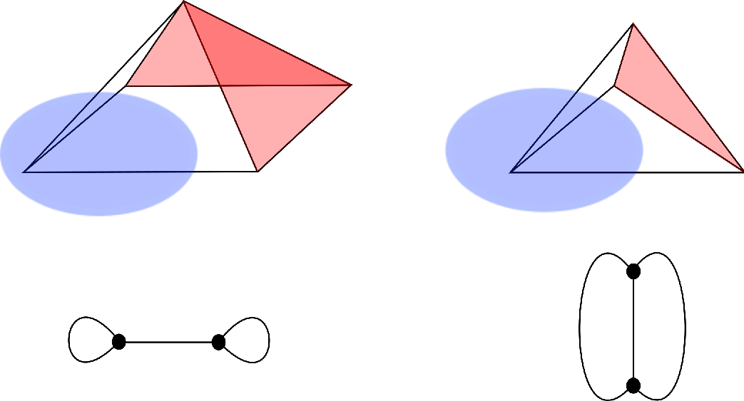
Refer to caption
Figure 15. The two compactifications of 𝒳⁡(F2,S​L2​(ℂ))=ℂ3\mathcal{X}(F_{2},SL_{2}(\mathbb{C}))=\mathbb{C}^{3}.

Note that these polytopes agree outside of the highlighted facets, which correspond to the divisor DΓD_{\Gamma}.

9.4. Genus 33 curves

The trivalent genus 33 graphs are depicted in Figure 16. We analyze the algebra VCΓ​(S​L2​(ℂ))V_{C_{\Gamma}}(SL_{2}(\mathbb{C})) for Γ\Gamma the leftmost graph in Figure 16. The semigroup algebra ℂ⁡[HΓ∗]\mathbb{C}[H_{\Gamma}^{*}] is generated by the simple loops in this graph. Each of these loops xa​b​cx_{abc} is determined by the values a,b,ca,b,c on the outer edges in Figure 17.

Refer to caption
Figure 16. The trivalent graphs of genus 3.3.
∙\textstyle{\bullet}∙\textstyle{\bullet}∙\textstyle{\bullet}∙\textstyle{\bullet}a\textstyle{a}b\textstyle{b}c\textstyle{c}

Figure 17. The diagram representing xa​b​cx_{abc}.

The generating relation is x111​x100​x010​x001=x110​x101​x011​x000.x_{111}x_{100}x_{010}x_{001}=x_{110}x_{101}x_{011}x_{000}. We lift this by expanding the product x110​x101​x011​x000x_{110}x_{101}x_{011}x_{000} with skein relations.

x111​x100​x010​x001−x110​x101​x011​x000+x1102​x0002+x1012​x0002+x0112​x0002x_{111}x_{100}x_{010}x_{001}-x_{110}x_{101}x_{011}x_{000}+x_{110}^{2}x_{000}^{2}+x_{101}^{2}x_{000}^{2}+x_{011}^{2}x_{000}^{2}
+x1002​x0002+x0102​x0002+x0012​x0002+x1112​x0002−4​x0004+x111​x100​x011​x000+x111​x010​x101​x000+x111​x001​x110​x000+x_{100}^{2}x_{000}^{2}+x_{010}^{2}x_{000}^{2}+x_{001}^{2}x_{000}^{2}+x_{111}^{2}x_{000}^{2}-4x_{000}^{4}+x_{111}x_{100}x_{011}x_{000}+x_{111}x_{010}x_{101}x_{000}+x_{111}x_{001}x_{110}x_{000}
+x100​x010​x110​x000+x100​x001​x101​x000+x010​x001​x011​x000=0+x_{100}x_{010}x_{110}x_{000}+x_{100}x_{001}x_{101}x_{000}+x_{010}x_{001}x_{011}x_{000}=0

The boundary divisor is defined by the equation x000=0x_{000}=0, yielding x111​x100​x010​x001=0.x_{111}x_{100}x_{010}x_{001}=0. Each of these generators can be translated into a trace-word by choosing the spanning tree in Γ\Gamma which misses the edges a,b,ca,b,c in Figure 17. The word associated to xa​b​cx_{abc} is then trace of the elements corresponding to the indices {a,b,c}\{a,b,c\} with value 1.1.

9.5. A genus gg case

Now we restrict ourselves to the set of graphs Υg\Upsilon_{g}, depicted in Figure 18. In [M4] the semigroup HΥg∗H_{\Upsilon_{g}}^{*} is shown to be generated by those weightings of level ≤2\leq 2, subject to quadratic relations in these generators. It follows that generators of VCΥg​(S​L2​(ℂ))V_{C_{\Upsilon_{g}}}(SL_{2}(\mathbb{C})) are disjoint unions of loops with edges of multiplicity at most 22, see Figure 19. Each of these elements has a pole of order 11 or 22 along the divisor DΥg⊂BCΥg​(S​L2​(ℂ)).D_{\Upsilon_{g}}\subset B_{C_{\Upsilon_{g}}}(SL_{2}(\mathbb{C})). We identify the generating elements with trace-words by selecting the spanning tree which misses the top edge of each loop in Figure 18 and the loops at the ends of the graph, and ordering these edges from left to right.

Refer to caption
Figure 18. The graph Υg\Upsilon_{g}.
Refer to caption
Figure 19. Ribbon representations of trace-words.

For an edge e∈E⁡(Υg)e\in E(\Upsilon_{g}) one can consider products of generators [w1]​[w2]∈UΥg[w_{1}][w_{2}]\in U_{\Upsilon_{g}} which have the same weight on ee. In this case the left hand sides of these generators with respect to ee can be exchanged, producing a relation [w1]​[w2]=[w1′]​[w2′][w_{1}][w_{2}]=[w_{1}^{\prime}][w_{2}^{\prime}], this type of relation is lifted by the operation depicted in Figure 20. In a similar manner, two loops may intersect in the diagram, these relations are lifted by the operation depicted in Figure 21. In [M4] it is shown that extensions of the quadratic relations, along with the exchanging relations at edges suffice to generate the relations in HΥg∗H_{\Upsilon_{g}}^{*}.

Refer to caption
Figure 20. Skein relation which resolves a crossing along an edge.
Refer to caption
Figure 21. Skein relation which resolves a crossing in a trinode.

10. Geometry of BC,p→​(S​L2​(ℂ))B_{C,\vec{p}}(SL_{2}(\mathbb{C})) and KC,p→​(S​L2​(ℂ))K_{C,\vec{p}}(SL_{2}(\mathbb{C}))

We describe the closed intersection stratification defined by the boundary divisor DΓ⊂BCΓ,p→Γ​(S​L2​(ℂ))D_{\Gamma}\subset B_{C_{\Gamma},\vec{p}_{\Gamma}}(SL_{2}(\mathbb{C})), and we show that the irreducible components of the compactification of S​p​e​c​(ℂ⁡[HΓ])Spec(\mathbb{C}[H_{\Gamma}]) defined by the Rees algebra ℂ⁡[HΓ∗]\mathbb{C}[H_{\Gamma}^{*}] are degenerations of the components of DΓ.D_{\Gamma}.

10.1. The ideals ISI_{S}

An ideal II in an algebra with a basis of planar Γ−\Gamma-tensors is called ”planar” if it has a basis of planar Γ\Gamma-tensors. Planar bases exist for any WCΓ,p→Γ​(S​L2​(ℂ))/I,W_{C_{\Gamma},\vec{p}_{\Gamma}}(SL_{2}(\mathbb{C}))/I, for II any planar ideal.

Definition 10.1.

For S⊂V⁡(Γ),S\subset V(\Gamma), the ideal IS⊂WCΓ,p→Γ​(S​L2​(ℂ))I_{S}\subset W_{C_{\Gamma},\vec{p}_{\Gamma}}(SL_{2}(\mathbb{C})) is defined to be the homogenous ideal with L−L-th component the span of those Γ−\Gamma-tensors with <L<L paths through some vi∈S.v_{i}\in S.

Proposition 10.2.

The ideal IS⊂WCΓ,p→Γ​(S​L2​(ℂ))I_{S}\subset W_{C_{\Gamma},\vec{p}_{\Gamma}}(SL_{2}(\mathbb{C})), is prime and planar.

Proof.

Primeness of ISI_{S} follows from the observation that the product of two Γ\Gamma-tensors V⁡(P1,ϕ1,A1),V(P_{1},\phi_{1},A_{1}), V⁡(P2,ϕ2,A2)V(P_{2},\phi_{2},A_{2}) of levels L1,L2L_{1},L_{2} respectively at vv must have L1+L2L_{1}+L_{2} paths through v.v. Expanding a Γ−\Gamma-tensor in ISI_{S} by skein relations gives planar Γ−\Gamma-tensors in IS,I_{S}, as the resulting planar Γ−\Gamma-tensors have strictly smaller associated spin diagrams, this proves that ISI_{S} is planar. ∎

It follows that the graded component IS​(L)I_{S}(L) has a basis of those planar Γ−\Gamma-tensors with <L<L paths through some vertex in S.S. The component WCΓ,p→Γ​(L)/IS​(L)W_{C_{\Gamma},\vec{p}_{\Gamma}}(L)/I_{S}(L) has a basis of planar Γ−\Gamma-tensors which have exactly LL paths through each vertex in S,S, and ≤L\leq L paths through each v∈V⁡(Γ)∖Sv\in V(\Gamma)\setminus S. Multiplication in WCΓ,p→Γ​(S​L2​(ℂ))/ISW_{C_{\Gamma},\vec{p}_{\Gamma}}(SL_{2}(\mathbb{C}))/I_{S} is computed by expanding a product into planar Γ−\Gamma-tensors, and removing any summand with <L<L paths through some vertex in SS. The 00-locus DSD_{S} of ISI_{S} is ∩v∈SDv\cap_{v\in S}D_{v} as IS=∑v∈SIvI_{S}=\sum_{v\in S}I_{v}.

The scheme P​r​o​j​(ℂ⁡[HΓ∗])Proj(\mathbb{C}[H_{\Gamma}^{*}]) is S​p​e​c​(ℂ⁡[HΓ])Spec(\mathbb{C}[H_{\Gamma}]) compactified by a divisor KΓ,K_{\Gamma}, by arguments which are identical to those used for VCΓ,p→Γ​(S​L2​(ℂ))V_{C_{\Gamma},\vec{p}_{\Gamma}}(SL_{2}(\mathbb{C})) and WCΓ,p→Γ​(S​L2​(ℂ)).W_{C_{\Gamma},\vec{p}_{\Gamma}}(SL_{2}(\mathbb{C})). The ideals JS⊂ℂ⁡[HΓ∗]J_{S}\subset\mathbb{C}[H_{\Gamma}^{*}] which cut out the irreducible components KS⊂KΓK_{S}\subset K_{\Gamma} have an identical description to the ISI_{S} as vector spaces, following the bijection between planar Γ−\Gamma-tensors and spin diagrams.

Proposition 10.3.

Each DSD_{S} has a degeneration to the toric scheme KSK_{S}.

Proof.

The algebras ℂ⁡[DS]\mathbb{C}[D_{S}] and ℂ⁡[KS]\mathbb{C}[K_{S}] have matching planar bases. Multiplication in ℂ⁡[DS]\mathbb{C}[D_{S}] is computed by expanding the product in WCΓ,p→Γ​(S​L2​(ℂ))W_{C_{\Gamma},\vec{p}_{\Gamma}}(SL_{2}(\mathbb{C})), and cutting off terms with <L<L paths through some vertex in SS, a process which does not eliminate the highest term. The associated graded algebra of ℂ⁡[DS]\mathbb{C}[D_{S}] by the filtration defined by any x∈𝒞Γx\in\mathcal{C}_{\Gamma} with x⁡(e)≠0x(e)\neq 0 for all e∈E⁡(Γ)e\in E(\Gamma) is therefore ℂ⁡[KS]\mathbb{C}[K_{S}]. ∎

Corollary 10.4.

The scheme KV⁡(Γ)K_{V(\Gamma)} is isomorphic to DV⁡(Γ)D_{V(\Gamma)}

Proof.

The ideal IV⁡(Γ)I_{V(\Gamma)} has a basis of those planar Γ\Gamma tensors which are not maximal level for some v∈V⁡(Γ)v\in V(\Gamma). The coordinate ring ℂ⁡[DV⁡(Γ)]=WCΓ,p→Γ​(S​L2​(ℂ))/IV⁡(Γ)\mathbb{C}[D_{V(\Gamma)}]=W_{C_{\Gamma},\vec{p}_{\Gamma}}(SL_{2}(\mathbb{C}))/I_{V(\Gamma)} is therefore spanned by planar Γ\Gamma-tensors which are maximal everywhere in Γ.\Gamma. When the product V⁡(Pw,ϕw,Aw)​V​(Pw′,ϕw′,Aw′)V(P_{w},\phi_{w},A_{w})V(P_{w^{\prime}},\phi_{w^{\prime}},A_{w^{\prime}}) is expanded into V⁡(Pw+w′,ϕw+w′,Aw+w′)V(P_{w+w^{\prime}},\phi_{w+w^{\prime}},A_{w+w^{\prime}}) plus lower planar Γ−\Gamma-tensors, all of the lower summands are cut off. This is precisely the affine semigroup multiplication in ℂ⁡[HΓ∗]/JV⁡(Γ)\mathbb{C}[H_{\Gamma}^{*}]/J_{V(\Gamma)}. ∎

10.2. The stratification of KCΓ,p→Γ​(S​L2​(ℂ))K_{C_{\Gamma},\vec{p}_{\Gamma}}(SL_{2}(\mathbb{C}))

We construct the strata of the scheme KCΓ,p→Γ​(S​L2​(ℂ))K_{C_{\Gamma},\vec{p}_{\Gamma}}(SL_{2}(\mathbb{C})) by taking UnU^{n} quotients of each of the DS.D_{S}. The scheme ES=DS/UnE_{S}=D_{S}/U^{n} is cut out of KCΓ,p→Γ​(S​L2​(ℂ))K_{C_{\Gamma},\vec{p}_{\Gamma}}(SL_{2}(\mathbb{C})) by the ideal ISUn=IS∩VCΓ,p→Γ​(S​L2​(ℂ))I_{S}^{U^{n}}=I_{S}\cap V_{C_{\Gamma},\vec{p}_{\Gamma}}(SL_{2}(\mathbb{C})). This is the planar ideal in VCΓ,p→Γ​(S​L2​(ℂ))V_{C_{\Gamma},\vec{p}_{\Gamma}}(SL_{2}(\mathbb{C})) with a basis given by those planar Γ−\Gamma-tensors in ISI_{S} which have only [UP] orientations at their leaves. In particular, the stratification poset of KCΓ,p→Γ​(S​L2​(ℂ))K_{C_{\Gamma},\vec{p}_{\Gamma}}(SL_{2}(\mathbb{C})) by the ESE_{S} is isomorphic to the stratification poset defined by the DS.D_{S}.

We address when IS=ITI_{S}=I_{T} for distinct subsets S,T⊂V⁡(Γ).S,T\subset V(\Gamma). To simplify our arguments, we treat the case of KCΓ,p→Γ​(S​L2​(ℂ))K_{C_{\Gamma},\vec{p}_{\Gamma}}(SL_{2}(\mathbb{C})) and the semigroup UΓ∗U_{\Gamma}^{*}, however everything we say transfers immediately to BCΓ,p→Γ​(S​L2​(ℂ))B_{C_{\Gamma},\vec{p}_{\Gamma}}(SL_{2}(\mathbb{C})) and the semigroup HΓ∗.H_{\Gamma}^{*}.

Lemma 10.5.

The stratification poset of KCΓ,p→Γ​(S​L2​(ℂ))K_{C_{\Gamma},\vec{p}_{\Gamma}}(SL_{2}(\mathbb{C})) defined by the ESE_{S} is isomorphic to the stratification poset of P​r​o​j​(ℂ⁡[UΓ∗])Proj(\mathbb{C}[U_{\Gamma}^{*}]) by the components defined by the corresponding toric ideals.

Proof.

This follows from the planarity of the ideals ISU−nI_{S}^{U_{-}^{n}} and Proposition 10.3. ∎

Corollary 10.6.

For S⊂V⁡(Γ),S\subset V(\Gamma), if there is a spin diagram a∈UΓ​(L)a\in U_{\Gamma}(L) with the property that the sum a⁡(e)+a⁡(f)+a⁡(g)a(e)+a(f)+a(g) for the edges e,f,ge,f,g around a vertex v∈V⁡(Γ)v\in V(\Gamma) is 2​L2L precisely when v∈S,v\in S, then ISI_{S} is distinct from all ITI_{T} with S⊂T.S\subset T.

We pass to the convex cone 𝒰Γ∗\mathcal{U}_{\Gamma}^{*} in ℝE⁡(Γ)×ℝ\mathbb{R}^{E(\Gamma)}\times\mathbb{R}, and use the fact that if a rational point can be found which satisfies the requirements of Corollary 10.6, it can be sufficiently multiplied to procure a spin diagram.

Proposition 10.7.

If Γ\Gamma has a leaf, then for any S⊂V⁡(Γ)S\subset V(\Gamma), there is a point in 𝒰Γ∗\mathcal{U}_{\Gamma}^{*} which satisfies the condition of Corollary 10.6.

Proof.

We let w∈𝒰Γ∗w\in\mathcal{U}_{\Gamma}^{*} be the weighting of level 33 which assigns each edge 2.2. Each vertex has the sum w⁡(e)+w⁡(f)+w⁡(g)=6w(e)+w(f)+w(g)=6, we show that the value of this sum can be lowered for vv in any given set of vertices. Fix v∈V⁡(Γ)v\in V(\Gamma), choose a simple path e1,…,eke_{1},\ldots,e_{k} from an edge e1e_{1} which borders vv to a leaf ek=ℓ.e_{k}=\ell. We obtain a new weighting from ww, by changing the weight along this path with some rational, sufficiently small ϵ.\epsilon.

w′(e1)=w(e1)−ϵ,w′(e2)=w(e2)+ϵ,…,w′(ek)=w(ek)±ϵw^{\prime}(e_{1})=w(e_{1})-\epsilon,w^{\prime}(e_{2})=w(e_{2})+\epsilon,\ldots,w^{\prime}(e_{k})=w(e_{k})\pm\epsilon

This does not change the total sum around any vertex, except vv, which has its total sum lowered by ϵ.\epsilon. We can inductively repeat this procedure for all vertices in V⁡(Γ)∖SV(\Gamma)\setminus S to produce the required weighting. ∎

We can adapt the proof of Proposition 10.7 to prove the following for graphs without leaves.

Proposition 10.8.

If S⊂V⁡(Γ)S\subset V(\Gamma) has a pair of points connected by a simple path of odd length, then there is an element in UΓ∗U_{\Gamma}^{*} which satisfies the condition of Corollary 10.6. If Γ\Gamma has an odd length simple cycle, then for all S⊂V⁡(Γ)S\subset V(\Gamma), there is a point in 𝒰Γ∗\mathcal{U}_{\Gamma}^{*} which satisfies the condition of Corollary 10.6.

Proof.

The idea is the same as the proof of Proposition 10.7, we can construct paths from any vertex to the odd length cycle, or a node which has already been ”lowered”. We then observe that if v,w∈V⁡(Γ)v,w\in V(\Gamma) are seperated by a path of odd length, their total sums can be simultaneously lowered by shrinking the weight on the first, respectively last edges in such a path by a common ϵ,\epsilon, and placing alternating ±ϵ\pm\epsilon on the edges in between. ∎

∙\textstyle{\bullet}∙\textstyle{\bullet}∙\textstyle{\bullet}∙\textstyle{\bullet}∙\textstyle{\bullet}∙\textstyle{\bullet}−2​ϵ\textstyle{-2\epsilon}2​ϵ\textstyle{2\epsilon}−2​ϵ\textstyle{-2\epsilon}ϵ\textstyle{\epsilon}−ϵ\textstyle{-\epsilon}ϵ\textstyle{\epsilon}∙\textstyle{\bullet}∙\textstyle{\bullet}∙\textstyle{\bullet}∙\textstyle{\bullet}∙\textstyle{\bullet}−2​ϵ\textstyle{-2\epsilon}2​ϵ\textstyle{2\epsilon}−ϵ\textstyle{-\epsilon}ϵ\textstyle{\epsilon}−ϵ\textstyle{-\epsilon}

Figure 22. Changing the weighting along a path to an odd cycle.

If Γ\Gamma has only even length simple cycles, ESE_{S} is distinct from each ETE_{T} for S⊂TS\subset T, if V⁡(Γ)∖SV(\Gamma)\setminus S contains a pair of points an odd distance apart. Notice that this condition is heritable, if S⊂TS\subset T and SS has this property, then so does TT. Furthemore if SS does not have this property, then neither does R⊂SR\subset S.

Proposition 10.9.

If Γ\Gamma is bipartite with no leaves, then the lattice formed by the DSD_{S} is the quotient of the Boolean lattice on V⁡(Γ)V(\Gamma) by the ideal of those S⊂V⁡(Γ)S\subset V(\Gamma) such that V⁡(Γ)∖SV(\Gamma)\setminus S is contained in one of the sets in the partition B1∪B2=V⁡(Γ)B_{1}\cup B_{2}=V(\Gamma) defined by the bipartite structure.

Proof.

We have already shown that if V⁡(Γ)∖SV(\Gamma)\setminus S has an odd length path, we can distinguish ESE_{S} from other strata. This is not the case if and only if V⁡(Γ)∖SV(\Gamma)\setminus S is contained in a set of the partition, say B1B_{1}. The graph Γ\Gamma is regular, therefore |B1|=|B2||B_{1}|=|B_{2}|. If we assign weights to E⁡(Γ)E(\Gamma), The total sums of the weights around the vertices in B1B_{1} equals this same sum for B2B_{2}. It follows that if w∈𝒰Γ​(L)w\in\mathcal{U}_{\Gamma}(L) assigns all the vertices of B2B_{2} weight 2​L2L, the same must be the case for all vertices in B1B_{1}. ∎

It remains to determine the dimensions of each of the ES,E_{S}, we do this by calculating the dimensions of the corresponding faces of the polytope 𝒰Γ​(L).\mathcal{U}_{\Gamma}(L). First we describe 𝒰Γ​(L)\mathcal{U}_{\Gamma}(L) in a more convenient way. We choose a set of gg edges {e1,…,eg}\{e_{1},\ldots,e_{g}\}, which give a tree 𝒯\mathcal{T} when they are split {e1,e1′,…,eg,eg′}\{e_{1},e_{1}^{\prime},\ldots,e_{g},e_{g}^{\prime}\}, this defines a covering π:𝒯→Γ.\pi:\mathcal{T}\to\Gamma. We Choose a leaf ℓn\ell_{n} of Γ\Gamma, and set this to be a sink in 𝒯\mathcal{T} by placing a direction on all edges in 𝒯\mathcal{T} toward ℓn.\ell_{n}.

∙\textstyle{\bullet}∙\textstyle{\bullet}∙\textstyle{\bullet}∙\textstyle{\bullet}∙\textstyle{\bullet}∙\textstyle{\bullet}ℓ2\textstyle{\ell_{2}}ℓ1\textstyle{\ell_{1}}e1\textstyle{e_{1}}e1∗\textstyle{e_{1}^{*}}

Figure 23. Introducing a direction on 𝒯.\mathcal{T}.

We introduce slack variables, LvL_{v} , v∈V⁡(Γ)v\in V(\Gamma) at the vertices of Γ,\Gamma, and we identify 𝒰Γ​(L)\mathcal{U}_{\Gamma}(L) with the labellings ww of E⁡(𝒯)E(\mathcal{T}) which satisfy the triangle inequalities at each trinode, w⁡(ei)=w⁡(ei′)w(e_{i})=w(e_{i}^{\prime}), and w⁡(ev)+w⁡(fv)+w⁡(hv)=Lvw(e_{v})+w(f_{v})+w(h_{v})=L_{v}, Lv≤L.L_{v}\leq L. The value of a ww on 𝒯\mathcal{T} is determined by the LvL_{v} and the edges e1,…,eg,ℓ1,…,ℓn−1.e_{1},\ldots,e_{g},\ell_{1},\ldots,\ell_{n-1}. The dimension of 𝒰Γ​(L)\mathcal{U}_{\Gamma}(L) is E⁡(Γ)E(\Gamma), so no linear relations hold among these parameters. Forgetting for a moment that w⁡(ei)=w⁡(ei′),w(e_{i})=w(e_{i}^{\prime}), the value of ww on ℓn\ell_{n} is a linear combination of the Lv,w⁡(ei),w⁡(ei′),w⁡(ℓi)L_{v},w(e_{i}),w(e_{i}^{\prime}),w(\ell_{i}), with all coefficients equal to ±1,\pm 1, with the following signs.

  1. (1)

    The coefficient of the w⁡(ei),w⁡(ei′),w⁡(ℓk)w(e_{i}),w(e_{i}^{\prime}),w(\ell_{k}) is equal to (−1)d+1,(-1)^{d+1}, where dd is the length of the directed path containing the leaf and ℓn.\ell_{n}.

  2. (2)

    The coefficient of LvL_{v} is equal to (−1)d+1(-1)^{d+1}, where dd is the length of the directed path which starts at vv and includes ℓn.\ell_{n}.

If we pass to the face corresponding to EV⁡(Γ)E_{V(\Gamma)}, we set all LvL_{v} equal to LL. The result is freely determined by n+g−1=|E⁡(Γ)|−|V⁡(Γ)|n+g-1=|E(\Gamma)|-|V(\Gamma)| parameters. This allows us to prove the following result on EΓ.E_{\Gamma}.

Proposition 10.10.

If Γ\Gamma has a leaf, for any S⊂V⁡(Γ)S\subset V(\Gamma), the codimension of ESE_{S} is |S||S|

Proof.

This follows from the fact that each ESE_{S} is distinct, and c​o​d​i​m​(EV⁡(Γ))=|V⁡(Γ)|.codim(E_{V(\Gamma)})=|V(\Gamma)|. ∎

If Γ\Gamma has no leaves we can repeat the above construction for w∈𝒰Γ​(L)w\in\mathcal{U}_{\Gamma}(L), expressing w⁡(e1)w(e_{1}) as a linear combination of w⁡(ei),w⁡(ei∗),w⁡(e1∗)w(e_{i}),w(e_{i}^{*}),w(e_{1}^{*}) and the Lv.L_{v}. If the edge which gives e1,e1∗e_{1},e_{1}^{*} lies in a simple cycle of odd length, then the coefficient of w⁡(e1∗)w(e_{1}^{*}) is −1-1. It follows that w⁡(e1),w⁡(e1∗),…,w⁡(eg),w⁡(eg∗)w(e_{1}),w(e_{1}^{*}),\ldots,w(e_{g}),w(e_{g}^{*}) satisfy a linear equation when the LvL_{v} are set to LL. As a consequence c​o​d​i​m​(EV⁡(Γ))=|V⁡(Γ)|codim(E_{V(\Gamma)})=|V(\Gamma)| in this case. If Γ\Gamma has no leaves and is bipartite, the coefficient of w⁡(ei)w(e_{i}) in the expansion of w⁡(e1)w(e_{1}) is opposite of that of w⁡(ei∗)w(e_{i}^{*}), and the coefficient of w⁡(e1)w(e_{1}) is 1.1. It follows that when all LvL_{v} are set to LL, the remaining parameters satisfy no linear equations. The following finishes the proof of Theorem 1.6.

Proposition 10.11.

If Γ\Gamma has no leaves, but has a simple cycle of odd length, ESE_{S} for any S⊂V⁡(Γ)S\subset V(\Gamma) has codimension |S|.|S|. If Γ\Gamma is bipartite and has no leaves, ESE_{S} has codimension |S||S| if V⁡(Γ)∖SV(\Gamma)\setminus S is not contained in partition set BiB_{i}, and 2​g−32g-3 otherwise.

Proof.

By Propositions 10.8 and 10.9 and the argument above, it remains to observe that there is a complete flag of subsets of V⁡(Γ)V(\Gamma), such that no subset of size ≥2\geq 2 is contained in a partition set BiB_{i}. ∎

Refer to caption
Figure 24. A non-Boolean stratification poset.

References

  • [A] T. Abe, Projective normality of the moduli space of rank 2 vector bundles on a generic curve, Transactions AMS, (2010), 362, 477-490.
  • [AB] V. Alexeev and M. Brion, Toric degenerations of spherical varieties, Selecta Mathematica, (2005), 10, 4, 453-478.
  • [Ba] J. Baez, An Introduction to Spin Foam Models of BF Theory and Quantum Gravity, Lect. Notes Phys. (2000), 543, 25-94.
  • [B1] A. Beauville, Conformal Blocks, Fusion Rules, and the Verlinde formula, Proceedings of the Hirzebruch 65 Conference on Algebraic Geometry, Israel Math. Conf. Proc., 9, Bar-Ilan Univ., Ramat Gan (1996), 75–96.
  • [BL] A. Beauville, Y. Lazlo, Conformal Blocks and Generalized Theta Functions, Math. Phys. 164 (1994) 385-419.
  • [BBH] U. Bhosle, I. Biswas, J. Hurtubise, Grassmannian framed bundles and generalized parabolic structures, arXiv:1202.4239 [math.AG]
  • [Bh] U. Bhosle, Parabolic vector bundles on curves, Ark. Mat. (1989), 27, 15-22.
  • [Bu] W. Buczyńska, Phylogenetic toric varieties on graphs, J. Algebraic Comb. (2012), 35, 3, 421-460.
  • [BBKM] W. Buczyńska, J. Buczyński, K. Kubjas, and M. Michalek, Degrees of generators of phylogenetic semigroups on graphs, arXiv:1105.5382v1 [math.CO].
  • [BW] W. Buczyńska and J. Wieśniewski, On the geometry of binary symmetric models of phylogenetic trees, JEMS. (2007), 9, 609-635.
  • [DM] P. Deligne, D. Mumford, The irreducibility of the space of curves of given genus, Publications Mathématiques de l’IHÉS, (1969), 36, 75-109.
  • [Fal] G. Faltings, A proof of the Verlinde formula, J. Algebraic Geometry (1994), 3, 347-374.
  • [F] C. Florentino, Schottky uniformization and vector bundles over Riemann surfaces, Manuscripta Mathematica (2001), 105, 1, 69-83.
  • [FL] C. Florentino, S. Lawton, Character varieties and the moduli quiver representations, to appear: Papers from 5th Ahlfors-Bers Colloquium, Rice University, Contemp. Math. AMS, 2013.
  • [FG] V.V. Fock, A.B. Goncharov, Moduli spaces of local systems and higher Teichmuller theory, Publications Mathématiques de l’IHÉS, (2006), 203, 1–211.
  • [FH] W. Fulton, J. Harris, Representation Theory, GTM, Vol. 129, Springer, Berlin, (1991).
  • [Gi] D. Gieseker, A degeneration of the moduli space of stable bundles, J. Differential Geom, (1984), 19, 1, 173-206.
  • [G1] W. Goldman, Invariant functions on Lie groups and Hamiltonian flows of surface group representations, Invent. Math. (1986), 85, 263-302.
  • [G2] W. Goldman, The symplectic nature of fundamental groups of surfaces, Advances in Math. (1980), 54, 200-225.
  • [Gr] F.D. Grosshans, Algebraic homogeneous spaces and invariant theory, Springer Lecture Notes, vol. 1673, Springer, Berlin, (1997).
  • [HJ] J. Hurtubise, L. Jeffrey, Representations with weighted frames and framed parabolic bundles, Canad. J. Math. (2000), 52, 6, 1235-1268.
  • [HJS] J. Hurtubise, L. Jeffrey and R. Sjamaar, Moduli of framed parabolic sheaves, Ann. Global Anal. Geom. 28 (2005) 351-370.
  • [JW] L. Jeffrey, J. Weitsman, Bohr-Sommerfeld Orbits in the Moduli Space of Flat Connections and the Verlinde Dimension Formula, Commun. Math. Phys. (1992), 150, 593-630.
  • [KMSW] A.N. Kirillov, P. Mathieu, D. Senechal, and M.A. Walton, Crystalizing the depth rule and WZNW fusion coefficients, Proceedings of the XIXth International Colloquium on Group Theoretical Physics, Salamanca, Spain, (1992).
  • [Kir] F. C. Kirwan, Symplectic implosion and nonreductive quotients, Geometric Aspects of Analysis and Mechanics, Progress in Mathematics, (2011), 292, 213-256.
  • [KM] K. Kubjas, C. Manon, Conformal blocks, Berenstein-Zelevinksy triangles, and group-based models, J. Algebraic Comb. (2014), 40, 3, 861-886.
  • [Ku] S. Kumar, Demazure character formula in arbitrary Kac-Moody setting, Invent. Math. (1987) 89, 395-423 .
  • [KNR] S. Kumar, M.S. Narasimhan, A. Ramanathan, Infinite Grassmannians and moduli spaces of G-bundles, Math. Annalen, (1994), 300, 41-75.
  • [LP] S. Lawton, E. Peterson, Computing S​L​(2,C)SL(2;C) Central Functions with Spin Networks, Geometriae Dedicata, (2011), 153, 1, 73-105.
  • [LS] Y. Lazlo and C. Sorger, The line bundles on the moduli of parabolic G-bundles over curves and their sections, Ann. Sci. Ecole Norm. Sup. (1997), 30, 4, 499-525.
  • [L] E. Looijenga, Conformal blocks revisited, arXiv:math/0507086v1 [math.AG]
  • [M4] C. Manon, The algebra of conformal blocks, arXiv:0910.0577 [math.AG]
  • [M7] C. Manon, Coordinate rings for the moduli of S​L2​(ℂ)SL_{2}(\mathbb{C}) quasi-parabolic principal bundles on a curve and toric fiber products, J. Algebra, (2011) 365, 1, 163-183.
  • [M10] C. Manon, The algebra of S​L3​(ℂ)SL_{3}(\mathbb{C}) conformal blocks, Trans. Groups, (2013), 18, 4, 1165-1187.
  • [M16] C. Manon, Toric geometry of S​L2​(ℂ)SL_{2}(\mathbb{C}) free group character varieties from outer space, arXiv:1410.0072 [math.AG]
  • [Mu] D. Mumford, Geometric Invariant Theory, Ergebnisse der Mathematik und Ihrer Grenzgebiete, (1965), 34, Springer.
  • [MSW] G. Musiker, R. Schiffler, L. Williams, Bases for cluster algebras form surfaces, Compositio Math. (2013) 149, 2, 217-263
  • [NS] M. S. Narasimhan, C. S. Seshadri, Stable and unitary vector bundles on a compact Riemann surface, Ann. of Math. (1965), 82, 540-567.
  • [NaS] D. S. Nagaraj, C. S. Seshadri, Degenerations of the moduli spaces of vector bundles on curves. II. Generalized Gieseker moduli spaces, Proc. Indian Acad. Sci. Math. Sci. (1999), 109, 2, 165–201.
  • [P] C. Pauly, Espaces de modules de fibrés paraboliques et blocs conformes, Duke Mathematical Journal (1996), 84, 217-235.
  • [PS] J.H. Przytycki, A. Sikora, On Skein Algebras and S​L2​(ℂ)−SL_{2}(\mathbb{C})-Character Varieties, Topology (2000), 39, 1, 115-148.
  • [RW] J. Rasmussen, M A Walton, Affine su(3) and su(4) fusion multiplicities as polytope volumes, J. Phys A, (2002), 35, 32, 6939- 6952.
  • [St] B. Sturmfels, Grobner bases and convex polytopes, Lecture notes series 8, AMS, Providence, Rhode Island, (1996).
  • [StV] B. Sturmfels and M. Velasco, Blow-ups of ℙn−3\mathbb{P}^{n-3} at nn points and spinor varieties, J. Commutative Algebra (2010), 2, 223-244.
  • [StXu] B. Sturmfels and Z. Xu, Sagbi Bases of Cox-Nagata Rings, JEMS. (2010), 12, 2, 429-459.
  • [TUY] A. Tsuchiya, K. Ueno, and Y. Yamada, Conformal field theory on universal family of stable curves with gauge symmetries, Adv. Studies in pure Math. (1989), 19, 459-566.
  • [U] K. Ueno, Introduction to conformal field theory with gauge symmetry, Fields Institute Monographs; Vo. 24. (2008).

Christopher Manon:
Department of Mathematics,
George Mason University
Fairfax, VA 22030 USA