The H molecular ion: low-lying states
Abstract
Matching for a wavefunction the WKB expansion at large distances and Taylor expansion at small distances leads to a compact, few-parametric uniform approximation found in J. Phys. B44, 101002 (2011). The ten low-lying eigenstates of H of the quantum numbers with at , with , and , at of both parities are explored for all interproton distances . For all these states this approximation provides the relative accuracy (not less than 5 s.d.) locally, for any real coordinate in eigenfunctions, when for total energy it gives 10-11 s.d. for a.u. Corrections to the approximation are evaluated in the specially-designed, convergent perturbation theory. Separation constants are found with not less than 8 s.d. The oscillator strength for the electric dipole transitions is calculated with not less than 6 s.d. A dramatic dip in the oscillator strength at is observed. The magnetic dipole and electric quadrupole transitions are calculated for the first time with not less than 6 s.d. in oscillator strength. For two lowest states (or, equivalently, and states) the potential curves are checked and confirmed in the Lagrange mesh method within 12 s.d. Based on them the Energy Gap between and potential curves is approximated with modified Pade with not less than 4-5 figures at a.u. Sum of potential curves is approximated by Pade in a.u. with not less than 3-4 figures.
pacs
31.15.Pf,31.10.+z,32.60.+i,97.10.LdINTRODUCTION
The H molecular ion is the simplest molecular system which exists in Nature. It plays a fundamental role in atomic-molecular physics, in laser and plasma physics being also a traditional example of two-center Coulomb system of two heavy Coulomb charges and electron, in Quantum Mechanics (see e.g. [1]). Due to the fact that the proton is much heavier than electron the problem is usually explored in the static approximation - the Bohr-Oppenheimer approximation of the zero order - where the protons are assumed to be infinitely heavy. In general, the projection of the angular momentum to the molecular axis (the line connecting the proton positions) is the integral, , where is the Hamiltonian. Thus, the angular variable can be separated out. Hence, the problem is reduced to two-dimensional, which admits itself the separation of variables in elliptic coordinates. It reflects the outstanding property of the general two-center Coulomb problem of the complete separation of variables in prolate ellipsoidal coordinates.
General two-center Coulomb problem can not be solved exactly, but approximately only. Thus, we need to introduce a definition of solvability of the spectral problem, of the corresponding Schrödinger equation: for all (or some) eigenfunctions we have to be able to find constructively an uniform approximation such that
| (1) |
in the coordinate space, while in vicinity of the nodal surface, , the absolute deviation
| (2) |
The parameter characterizes a number of significant digits (s.d.) in wavefunction at real , which the approximation reproduces exactly. It implies that any observable, any matrix element can be found with accuracy not less than . In principle, in the case of non-relativistic QED in the Born-Oppenheimer (static) approximation we think that is sufficient to get physically-relevant results: the corrections due to finite proton mass, its form factor, relativistic effects of different types are small; in particular, for energies of states they should contribute to significant digit 4,5,6 etc. Our aim is to solve the problem of H molecular ion in non-relativistic QED approximation by constructing maximally-simple, compact, locally-accurate approximations for the ten low-lying eigenfunctions.
The goal of this paper is to extend and profound the analysis in [2] for the states and and explore the eight more low lying states of the H molecular ion. In order to check accuracy of obtained approximations a convergent perturbation theory (PT) used in [2] is extended for the case of excited states. This PT allows us to evaluate a local deviation of the approximation from the exact eigenfunction. Eventually, we calculate systematically separation constants and the oscillator strength for the electric dipole and quadrupole, and magnetic dipole transitions.
It is worth mentioning that a study of the wavefunctions of the H molecular ion in a form of expansion in some basis was initiated a long ago by Hylleraas [3], and it was successfully realized in the remarkable paper [4] (see also [5, 6]). Since old times there were made many attempts to find bases leading to fast convergence. At present, the basis of pure exponential functions seems the most fast convergent (see e.g. [7] and references therein). Note that following the analysis of classical mechanics of the H system and its subsequent semiclassical quantization it was attempted a long ago to build some compact uniform approximations of wavefunctions of low lying electronic states [8]. Local accuracies of these approximations are unclear whilst eigenvalues are found with a few significant digits. We are unaware about further attempts in this direction except for our previous paper [2]. Note that a similar idea to construct compact uniform approximations of the lowest eigenfunctions was successfully realized for quartic anharmonic oscillator [9] and double-well potential [10].
Throughout the paper the Rydberg is used as the energy unit while for the other quantities standard atomic units are used .
I Generalities
The Schrödinger equation, which describes the electron in the field of two fixed centers of the charges at the distance , is of the form
| (3) |
where and the total energy are in Rydbergs, are the distances from electron to first (second) center, respectively, see Fig. 1. All distances are in a.u. From physical point of view, we study the motion of electron in the field of two Coulomb wells situated on the distance . Hence, if the wells become identical - any eigenstate should be characterized by a definite parity with respect to permutation of wells. Furthermore, at , when the barrier gets large and tunneling becomes exponentially-small, the phenomenon of pairing should occur: the spectra of positive parity states is almost degenerate with the spectra of negative parity states. For each pair the energy gap should be exponentially-small, .

Following [1] let us introduce the dimensionless 2D elliptic coordinates and azimuthal angle with respect to the molecular axis 11 1 From point of view they are prolate spheroidal.:
| (4) |
In these coordinates the Coulomb singularities are situated at
being at the boundaries of the configuration space. The Jacobian is . The equation (3) admits separation of variables in (4). Since the projection of the angular momentum to the molecular axis commutes with the Hamiltonian 22 2 Due to complete separation of variables one more integral in a form of the second order polynomial in momentum exists [11], it is closely related to Runge-Lenz vector [12] and commutes with ; hence, the H ion in adiabatic (Born-Oppenheimer) approximation is completely-integrable system. the eigenstate has a definite magnetic quantum number . If the Hamiltonian is permutationally-symmetric , or, equivalently, , hence, any eigenfunction is of a definite parity (). As a result, it can be represented in a form
| (5) |
where is of definite parity, . Following this analysis we introduce the notation for a state as where are the quantum numbers in and coordinates, respectively, they have a meaning of number of nodes in and , is a magnetic quantum number, while is parity. It is easy to check that the ground state with the lowest total energy is .
The factors and are introduced to (5) to take into account a singular behavior of the eigenfunction near Coulomb singularities in accordance to the boundary conditions. After substitution of the representation (5) into (3) we arrive at the equations for and ,
| (6) |
| (7) |
respectively, where following [4] we denote,
| (8) |
and is a separation constant. Equations (6), (7) define a bispectral problem with as spectral parameters for any given .
It is interesting that the operators in lhs of the equations (6), (7) are of the Lie-algebraic nature. After the gauge rotation
the operator can be rewritten in terms of the -Lie algebra generators
| (9) |
see e.g. [32], with
In a similar way after the gauge rotation
the operator can be rewritten in terms of the -Lie algebra generators (9) with
Hence, the hidden algebra of H molecular ion after separation of the angular variable in coordinates is [2]. The spin of the representation is and , respectively. For non-physical, integer, non-negative values of and integer ratio , each algebra appears in the finite-dimensional representation realized in action on polynomials in , respectively. It is worth noting that the operator (7) is -invariant: . Thus, it can be gauge-rotated with and then a new variable can be introduced,
it leads to another convenient representation of the Eq.(7).
Square-integrability of the function (5) implies a non-singular behavior of at and decay at as well as non-singular behavior of at . Such a non-singular solution can be continued from the interval to the whole line . It implies searching a solution of the spectral problem (6) which grows at , decays at being a constant at . A non-singular solution at can be unambiguously continued in beyond the interval to , it corresponds to growing (non-decaying) behavior of at .
The equation (6) formally coincides with equation (7) at (united atom limit). It is evident that if a domain for (7) is extended to it has no solutions since there is no degeneracy at any with . Hence, at the solution found solving the equation (6) should be non-normalizable. Since at the problem becomes one-center Coulomb problem and can be solved exactly. The above statement can be checked explicitly. It is in agreement with large -behavior of the celebrated Guillemin-Zener function, which mimics the coherent interaction of electron with charged centers, see e.g. [2]. It leads to
| (10) |
which eventually has to describe small behavior of the H. It is also in agreement with large -behavior of the celebrated Hund-Mulliken function (it mimics the incoherent interaction of electron with charged centers) for both (of positive parity) and (of negative parity) states, see e.g. [2],
| (11) |
which describes large behavior.
I.1 Asymptotics.
Assuming a representation , then the WKB-type-expansion of phase at can be derived,
| (12) |
while at ,
| (13) |
Similarly to if we assume , then at ,
| (14) |
when at ,
| (15) |
The important property of the expansions (12) and (14) is that the coefficients in front of the growing terms at large distances (linear and logarithmic) are found explicitly, since they do not depend on the separation constant .
I.2 Approximation
Making interpolation between WKB-type-expansion (12) and the perturbation theory (13) for , (14) and (15) for , correspondingly, and taking into account that the symmetry: of is realized through use of -function (cf. (11) and (10)) we arrive at the following expression [2]
| (16) |
for the eigenfunction of the state with the quantum numbers . Here and are parameters (see below), and are some polynomials of degrees and with real coefficients with and real roots in the intervals and , respectively. We will choose these polynomials in such a way to ensure their orthogonality to all states with lower total energies.
II Results
II.1 Ground state of positive/negative parity
In this Section we consider briefly two lowest states - one of positive and one of negative parity, and , respectively, updating the consideration which was done in [2]. Corresponding approximations for above states have the form
| (17) |
(cf.(16)), respectively, and each of them depends on six parameters and . The easiest way to choose these parameters is to make a variational calculation taking (17) as a trial function for fixed and with as an extra variational parameter. Immediate striking result of the variational study is that for all a.u. the optimal value of the parameter coincides with the exact value of (see (8)) with extremely high accuracy for both and states. It implies a very high quality of the trial function - the variational optimization wants to reproduce with very high accuracy a domain where the eigenfunction is exponentially small, hence, the domain which gives a very small contribution to the energy functional. In Tables 1 and 2 some selected results for the total energy (as well as for sensitive ) vs of and states are shown as well as their comparison with ones obtained by Montgomery [5] (in highly-accurate realization of the approach proposed by Bates et al [4]), and also with the results we obtained in the Lagrange mesh method based on Vincke-Baye approach [13] (for details and discussion see [14]). For all studied values of for both and states our variational energy turns out to be in agreement on the level of 10 s.d. with these two alternative calculations. Note that for a.u. the energies of and states coincide in 10 s.d. according to the pairing phenomenon. Also they differ from the ground state energy of Hydrogen atom a.u., this difference reduces gradually with further growth of .
The potential curve has a “flat” minimum at a.u. characterized by a small curvature, see Table 1. It defines the equilibrium distance : numerically, the value of agrees with [15] in all seven digits. The first non-vanishing term in a Taylor expansion of the potential curve around the minimum at is quadratic . Thus, the coefficient, proportional to the so-called harmonic force constant , see e.g. [15], is given by the expression
| (18) |
Making accurate calculations around minimum of the potential curve one can calculate . Not surprisingly, it coincides with value reported by Bishop [15] in all digits.
The potential curve, inside the accuracy of our calculations, displaces very “flat” and shallow minimum at a.u. , see Table 2, characterized by a small curvature. The depth of the minimum is Ry, if it is compared to the asymptotics of the potential curve (or, in other words, to the ground state energy of the Hydrogen atom). The existence to this minimum, due to the Van der Waals attraction at large distances between the Hydrogen atom and the proton, was demonstrated time ago (see e.g. [16] and references therein).
Variational parameters are smooth, slow-changing functions of , see Figure 2. Note that the number of optimization parameters can be reduced by putting . In this case the accuracy in energy drops from 10-11 to 5-6 s.d. - it is still acceptable from physics point of view being consistent with a domain of applicability of non-relativistic QED, see a discussion above. All calculations are implemented in double precision arithmetics and checked in quadruple precision one.
Hence, our relatively-simple, few parametric functions (17) taken as trial functions in a variational study provide extremely high accuracy in energy in comparison with highly-accurate alternative calculations usually much more demanding computationally. Two naturally related questions occur: (i) can we estimate the accuracy of variationally obtained energies without making a comparison with other calculations and (ii) how close locally our functions to the exact ones in configuration space. In order to answer these questions, we develop a perturbation theory in the Riccati equation derived from the Schrödinger equation (3) taking a trial function (17) as zero approximation, see [2] 33 3 Such a procedure is called no-linearization, see [33].
Let us choose (17) with parameters fixed via variational calculation (see above) as zero approximation in perturbation theory (58), (64) (see Appendix). For given one can calculate a potential , for which the approximation (17) is the exact eigenfunction. It is evident that by construction of the emerging perturbation theory has to be convergent: the perturbation potential is subdominant. Assuming the consistency condition (70) is fulfilled for the first corrections, namely, , we find the first corrections and as functions of . Then we modify the trial function (17) accordingly,
| (19) |
and make the variational calculation with this trial function minimizing with respect to parameter . The (expected) result is that the optimal value of parameter remained unchanged with respect to the value obtained for the trial function (17) with extremely high accuracy - within 10 s.d.! It indicates that the condition (70) is fulfilled with high accuracy. The variational energy is changed beyond the 10 s.d. Therefore, our energies presented in Tables 1, 2 are correct in all ten digits. The separation parameters are presented in Table 6 together with those corresponding to other states (see below). It allows us to find explicitly and . As an illustration the functions and are shown for a.u. on Figs. 7 and 8. Corrections and are shown in [2]. Similar behavior of corrections appears for all other values of .
| R[a.u.] | [Ry] (Present/[5]/Mesh) | |
|---|---|---|
| 1.0 | -0.90357262676 | 0.8519936 |
| -0.90357262676 | ||
| -0.90357262676 | ||
| 1.997193 | -1.20526923821 | 1.483403 |
| – | ||
| -1.20526923821 | ||
| 2.0 | -1.20526842899 | 1.485015 |
| -1.20526842899 | ||
| -1.20526842899 | ||
| 40.0 | -1.0000017622 | 20.4939 |
| —– | ||
| -1.0000017622 |
| R [a.u.] | (Present/[5]/Mesh) [Ry] | |
|---|---|---|
| 1.0 | 0.8703727499 | 0.5314196 |
| 0.8703727498 | ||
| 0.8703727498 | ||
| 1.997193 | -0.3332800331 | 1.1536645 |
| —– | ||
| -0.33328003316 | ||
| 12.54525 | -1.0001215811 | 6.75434 |
| — | ||
| -1.0001215811 | ||
| 40.0 | -1.0000017622 | 20.4939 |
| — | ||
| -1.0000017622 |


II.2 states with
As the further check the quality of the approximation (16) proposed in [2], we considered the states with magnetic quantum number and both parities . These four states , , and correspond to the states , , and in the united atom nomenclature, respectively. The approximation takes the form
| (20) |
for positive and negative parity, respectively; it depends on six free parameters and , as well as which can be taken as an extra variational parameter. Due to the presence of the last factor in the function (20) is orthogonal to (17). Taking (20) as a trial function and using the variational method, the optimized values of these parameters are obtained for each fixed value of the internuclear distance . The results for the total energy and the value of p for the states with and both parities as a function of the internuclear distance are presented in Table 3. For each -value, the second line are the results presented by Madsen and Peek [17]. In general, the agreement is on the level of s.d. except for a few values of where the agreement is on s.d. It can be clearly seen the pairing phenomenon, see Table 3: energies of the states of different parities approach to each other with growth of . At a.u. the energy gaps reach Ry and Ry for and states, respectively. The energy difference with appropriate state of Hydrogen atom, which occurs after dissociation, at , see e.g. Table 10, is Ry for a.u. This difference reduces gradually with further growth of .
In a similar way how it was done for ground states of the positive and negative parities (17) one can develop convergent perturbation theory for states individually, see Appendix, taking (20) as a zero approximation. Taking into account the first-order corrections to the function (20), it gets the form
| (21) |
The immediate striking observation is the first correction to energy is of order (or less) and influences digits beyond those shown in Table 3! On Figs. 9, 10, 11, 12, 13, 14, 15 and 16 the trial functions , and the first corrections to the phases and for a.u. are present. We must emphasize that the variational parameter in Table 3 coincides with the value of (8) found from the variational energy, on the level of 5 - 9 s.d. It indicates implicitly to a very high quality of the function (20).
| R[a.u.] | ||||||||
|---|---|---|---|---|---|---|---|---|
| 1.0 | 1.051 784 087 48(77) | 0.486 882 | 1.552 886 885 83 | 0.334 332 5 | 1.560 917 409 665 | 0.331 316 5 | 1.750 004 925 60 | 0.249 9975 |
| 1.051 784 087 4746 | 1.552 886 885 8238 | 1.560 917 409 6654 | 1.750 004 925 5960 | |||||
| 2.0 | 0.142 456 360 21(08) | 0.926 037 | 0.546 600 746 72 | 0.673 349 | 0.574 534 636 379 | 0.652 277 | 0.750 074 914 13 | 0.4999 25 |
| 0.142 456 360 20826 | 0.546 600 746 7126 | 0.574 534 636 3784 | 0.750 074 914 1264 | |||||
| 4.0 | -0.201 649 288 23 | 1.675 29 | 0.038 093 115 38 | 1.359 274 6 | 0.111 109 971 587 | 1.247 221 | 0.250 988 746 1 | 0.998 02 |
| -0.201 649 288 2302 | 0.038 093 115 3803 | 0.111 109 971 58626 | 0.250 988 746 0990 | |||||
| 6.0 | -0.260 649 791 31 | 2.312 11 | -0.121 744 444 93 | 2.0237 84 | -0.019 437 228 851 | 1.781 835 | 0.087 106 783 3 | 1.488 64 |
| -0.260 649 791 3114 | -0.121 744 444 95100 | -0.019 437 228 851128 | 0.087 106 783 24228 | |||||
| 8.0 | -0.269 021 262 54(37) | 2.881 725 | -0.188 783 036 57 | 2.649 628 | -0.071 453 569 562 | 2.267 87502 | 0.008 575 937 0 | 1.965 4 |
| -0.269 021 262 5382 | -0.188 783 036 58772 | -0.071 453 569 562040 | 0.008 575 936 87662 | |||||
| 10.0 | -0.265 432 580 28 | 3.411 13 | -0.219 833 749 01 | 3.239 73 | -0.095 093 601 175 | 2.716 126 | -0.035 171 033 8 | 2.424 722 |
| -0.265 432 580 2914 | -0.219 833 749 0582 | -0.095 093 601 17488 | -0.035 171 034 00198 | |||||
| 14.0 | -0.255 396 545 98 | 4.417 514 | -0.242 319 086 11 | 4.344 4 | -0.111 495 667 118 | 3.530 34 | -0.078 059 693 0 | 3.2901 3 |
| -0.255 396 546 2922 | -0.242 319 086 1426 | -0.111 495 667 11852 | -0.078 059 693 28034 | |||||
| 20.0 | -0.250 167 097 81 | 5.917 5 | -0.248 752 926 71 | 5.905 531 | -0.113 758 110 521 | 4.623 4 | -0.100 623 878 9 | 4.4791 1 |
| -0.250 167 098 9774 | -0.248 752 926 741 | -0.113 758 110 6214 | -0.100 623 879 14096 | |||||
| 30.0 | -0.249 755 905 14 | 8.437 72 | -0.249 734 619 46 | 8.437 4 | -0.110 960 223 7 | 6.322 | -0.109 116 195 2 | 6.28897 |
| -0.249 755 905 4846 | -0.249 734 619 4714 | -0.110 960 225 79684 | -0.109 116 195 34154 | |||||
| 40.0 | -0.249 872 858 88 | 10.952 1 | -0.249 872 610 06 | 10.952 1 | -0.110 588 155 | 8.014 7 | -0.110 429 620 8 | 8.01073 |
| -0.249 872 859 9708 | -0.249 872 610 0936 | -0.110 588 156 5852 | -0.110 429 620 89928 | |||||
| 50.0 | -0.249 928 750 05 | 13.461 3 | -0.249 928 747 50 | 13.461 26 | -0.110 756 575 | 9.706 8 | -0.110 745 830 0 | 9.7065 |
| -0.249 928 750 0956 | -0.249 928 747 5080 | -0.110 756 576 55914 | -0.110 745 830 06112 |
II.3 Ellipsoidal nodal surfaces: the states
The proposed approximation (16) [2] allows us to study the th excited state in direction with nodes in the variable. Let us consider the simplest states, , and both parities , i.e. the states or, differently, and , respectively. The main difference with the approximation for the ground state (17) comes due to the presence of a monomial factor in the expression for , while the remains functionally the same,
| (22) |
Here defines the position of the node and it can be fixed by imposing the orthogonality condition between these states ( parity) and the lowest states, i.e. . The orthogonality with the states for any is always fulfilled. Eventually, the approximation contains six free parameters which are obtained using the variational method. Results are presented in Table 4 for the two states and as a function of the internuclear distance . Comparison with previous, highly accurate results [17] (given on the second line) for each is presented. The agreement is on the level of s.d. For each state the variational value of (when is taken as a variational parameter in (16)) as well as the node position are given. It can be clearly seen on Table 4 the pairing phenomenon: energies of the states of opposite parities approach to each other with growth of . At a.u. the energy gap reaches a.u. for states. The energy difference with appropriate state of Hydrogen atom is a.u., see e.g. Table 10, for the case this difference should reduce gradually with further growth of .
In both cases the node position is a decreasing function of the internuclear distance having a finite value for small and conversely approaching to the lower limit in -coordinate, at large , roughly as . At the point , the wave function (22) vanishes. In the configuration space it corresponds to a nodal surface which is a prolate spheroid of eccentricity . Corrections to the node-position can be calculated developing a convergent perturbation theory (see Appendix, Eq.(62)). We found that for these two states the first correction is . Functions , and the first corrections to the phases are shown in Figs. 17, 18, 19 and 20 for a.u. as an illustration.
| R[a.u.] | ||||||
|---|---|---|---|---|---|---|
| 1.0 | 1.154 150 822 6 | 0.4598503 | 2.782853311 | 1.521 369 039 285 | 0.345916 | 5.360475264 |
| 1.154 150 823 003 | 1.521 369 039 2720 | |||||
| 2.0 | 0.278 270 249 325 | 0.849547 | 1.907869613 | 0.489 173 669 829 | 0.714721 | 2.532742379 |
| 0.278 270 249 323 4 | 0.489 173 669 8286 | |||||
| 4.0 | -0.077 029 734 913 5 | 1.5192495 | 1.477672193 | 0.009 780 899 90 | 1.40031296 | 1.589362953 |
| -0.077 029 734 914 98 | 0.009 780 899 904368 | |||||
| 6.0 | -0.161 775 845 624 | 2.11092 | 1.330973187 | -0.121 531 762 3 | 2.02331 | 1.364704127 |
| -0.161 775 845 629 74 | -0.121 531 762 33782 | |||||
| 8.0 | -0.193 554 665 734 | 2.663996 | 1.254298836 | -0.174 967 289 16 | 2.60758 | 1.265974957 |
| -0.193 554 665 735 18 | -0.174 967 289 19184 | |||||
| 10.0 | -0.209 421 251 79 | 3.1993 | 1.206019531 | -0.201 171 505 95 | 3.16691 | 1.210160770 |
| -0.209 421 251 818 4 | -0.201 171 506 037 | |||||
| 20.0 | -0.236 998 606 92 | 5.80516 | 1.103266490 | -0.236 904 750 195 | 5.80435 | 1.103289607 |
| -0.236 998 606 945 2 | -0.236 904 750 2114 | |||||
| 30.0 | -0.243 892 622 63 | 8.35918 | 1.068352565 | -0.243 891 770 96 | 8.35916 | 1.068352748 |
| -0.243 892 622 973 6 | -0.243 891 770 9742 | |||||
| 40.0 | -0.246 478 659 89 | 10.88997 | 1.051017992 | -0.246 478 652 70 | 10.88997 | 1.051017930 |
| -0.246 478 659 911 8 | -0.246 478 652 7404 | |||||
| 50.0 | -0.247 714 222 867 | 13.40975 | 1.040679396 | -0.247 714 222 80 | 13.40975 | 1.040679432 |
| -0.247 714 222 873 8 | -0.247 714 222 8160 |
II.4 states
Now, let us consider states with two nodes in the -coordinate at . These states correspond to or in the united atom notation and , respectively. The functional form of the function is the same as one of the ground state (17) while the function is given by
| (23) |
This contain a second-degree polynomial (cf. (16)) indicating the node positions which are fixed by the orthogonality condition to the states . The approximation contains six free parameters whose are going to be optimized by applying the variational method.
Table 5 presents the results for the total energy as well as the values of the -parameter and the node position . The nodes appear symmetrically with respect to . The node surfaces are hyperboloids of revolution around the internuclear axis with eccentricity . One can see in Table 5 there is a dramatic decrease in the accuracy of the variational energies of both states for small internuclear distances. When comparing the total energy of the state with the results presented by Madsen and Peek [17] (second row) we have 7 s.d. in agreement for a.u. dropping steadily to 4 s.d. for a.u. With regard to the state the agreement is in 8-9 s.d. for a.u. decreasing to 3-4 s.d. for a.u. It can be clearly seen on Table 5 the pairing phenomenon: energies of the states of different parities approach to each other with growth of . At a.u. the energy gap reaches Ry for states. The energy difference with appropriate state of the Hydrogen atom at is Ry, this difference should reduce gradually with further growth of .
Calculation of the 2nd correction to energy (and the first correction to the node positions) with Eq. (68), see Appendix, does not improve significantly the variational energies. The first correction to is very small. This is the indication to a slower convergence of the perturbation theory for those states compared to other states. It is evident that the pre-factor in (23), which describes nodes in (simple zeroes), should be more complicated than simply . For the moment, it is not clear in what direction it has to be modified.
| R[a.u.] | ||||||
|---|---|---|---|---|---|---|
| 1.0 | 1.549 645 | 0.33555 | 0.33559 | 1.749 201 | 0.2504 | 0.7750 |
| 1.549 630 623873 | 1.749 199 647 6496 | |||||
| 2.0 | 0.528 467 | 0.6867 | 0.34330 | 0.746 725 | 0.50328 | 0.7761 |
| 0.528 444 742349 | 0.746 712 259 7008 | |||||
| 4.0 | -0.071 447 03 | 1.51188 | 0.385086 | 0.235 14 | 1.0294 | 0.7813 |
| -0.071 447 5809595 | 0.235 095 441 5056 | |||||
| 6.0 | -0.291 656 30 | 2.37169 | 0.467547 | 0.041 358 | 1.621 | 0.7918 |
| -0.291 656 3202834 | 0.041 339 661 36794 | |||||
| 8.0 | -0.347 023 26 | 3.0907 | 0.55840 | -0.085 484 8 | 2.31685 | 0.8084 |
| -0.347 023 2833194 | -0.085 486 025 27608 | |||||
| 10.0 | -0.346 234 878 | 3.6954 | 0.633665 | -0.169 773 24 | 3.04045 | 0.828782 |
| -0.346 234 8809774 | -0.169 773 328 91252 | |||||
| 20.0 | -0.275 532 157 | 6.128 | 0.813436 | -0.261 170 845 7 | 6.00975 | 0.9032258 |
| -0.275 532 160827 | -0.261 170 846 1206 | |||||
| 30.0 | -0.257 715 275 | 8.543 | 0.873979 | -0.257 278 714 7 | 8.5374 | 0.934896 |
| -0.257 715 2848286 | -0.257 278 715 0364 | |||||
| 40.0 | -0.254 044 456 | 11.028 | 0.904351 | -0.254 036 841 34 | 11.02791 | 0.95097747 |
| -0.254 044 4736052 | -0.254 036 841 4156 | |||||
| 50.0 | -0.252 534 779 | 13.522 | 0.922873 | -0.252 534 676 43 | 13.52162 | 0.96066311 |
| -0.252 534 7813992 | -0.252 534 676 601 |
II.5 Separation constant
In developed perturbation theory so as to estimate the accuracy of the approximation (16) for and , two expressions, one for each variable, for the separation constant are derived, and (see Appendix and Eqs. (63) and (69)). They are not independent: the condition of consistency should be imposed. Table 6 presents the separation constant for all considered states. For each -value the first/second line correspond to / calculated with (63) / (69) compared to Madsen and Peek [17] (third row). It turns out that as a result of variational calculations the condition is fulfilled automatically, up to s. d. which is in agreement with those presented by Madsen and Peek [17]. Hence, there is no need to impose the equality condition. It is a reflection of the very high accuracy of the approximation (17).
| R[a.u.] | ||||||||
|---|---|---|---|---|---|---|---|---|
| 1.0 | 0.2499462430 | -1.8300104198 | 0.0476692616 | -3.9520464219 | 0.0157049965 | -5.9791583275 | 0.0711543055 | -1.9281072878 |
| 0.2499462409 | -1.8300104197 | 0.0476693150 | -3.9520464344 | 0.0157049889 | -5.9791583064 | 0.0711543140 | -1.9281072817 | |
| 0.2499462406113 | -1.830010419730 | 0.047669315711 | -3.952046434393 | 0.015704988875 | -5.979158306119 | 0.071154314127 | -1.928107280448 | |
| 2.0 | 0.8117295877 | -1.1868893947 | 0.1749484742 | -3.8048856116 | 0.0611354153 | -5.9165512457 | 0.2484661667 | -1.6917231809 |
| 0.8117295852 | -1.1868893929 | 0.1749484725 | -3.8048856050 | 0.0611354010 | -5.9165512311 | 0.2484661712 | -1.6917231733 | |
| 0.8117295846248 | -1.186889392359 | 0.174948472433 | -3.804885604702 | 0.061135400906 | -5.916551230876 | 0.248466171440 | -1.691723172798 | |
| 4.0 | 2.7995887561 | 1.5384644804 | 0.6001486772 | -3.1948053489 | 0.2270652065 | -5.6657454590 | 0.8535318015 | -0.7976034401 |
| 2.7995887582 | 1.5384644803 | 0.6001486748 | -3.1948053506 | 0.2270652107 | -5.6657454689 | 0.8535318003 | -0.7976034382 | |
| 2.799588759471 | 1.538464480300 | 0.600148674671 | -3.194805350518 | 0.227065210827 | -5.665745469006 | 0.853531800197 | -0.797603437898 | |
| 6.0 | 6.4536037434 | 5.9279301781 | 1.2199716980 | -2.1786687874 | 0.4743694112 | -5.2501595578 | 1.8115068883 | 0.5663869192 |
| 6.4536037423 | 5.9279301759 | 1.2199717011 | -2.1786687836 | 0.4743694166 | -5.2501595612 | 1.8115068932 | 0.5663869192 | |
| 6.453603742887 | 5.927930173726 | 1.219971701568 | -2.178668782566 | 0.474369416805 | -5.250159561131 | 1.811506894227 | 0.566386919545 | |
| 8.0 | 12.2261746132 | 12.0646853402 | 2.0537173294 | -0.7961022597 | 0.7914989890 | -4.6781903409 | 3.2069680505 | 2.3733521986 |
| 12.2261746118 | 12.0646853394 | 2.0537173246 | -0.7961022613 | 0.7914989805 | -4.6781903532 | 3.2069680527 | 2.3733521972 | |
| 12.22617461542 | 12.06468533824 | 2.053717323829 | -0.7961022613695 | 0.791498980083 | -4.678190353126 | 3.206968053370 | 2.373352197778 | |
| 10.0 | 20.1333096527 | 20.0921239053 | 3.1610270665 | 0.9355443423 | 1.1760019683 | -3.9601419353 | 5.1293596287 | 4.6288376336 |
| 20.1333042259 | 20.0921157054 | 3.1610270649 | 0.9355443394 | 1.1760019677 | -3.9601419604 | 5.1293596245 | 4.6288376291 | |
| 20.13329317839 | 20.09209890008 | 3.161027064845 | 0.9355443386850 | 1.176001967652 | -3.960141960690 | 5.129359623687 | 4.628837627894 | |
| 20.0 | 90.0528911866 | 90.0528775638 | 15.6431425753 | 15.4372141472 | 4.4202357771 | 1.6768434995 | 23.1467951638 | 23.1310108444 |
| 90.0528911837 | 90.0528775637 | 15.6431424784 | 15.4372141468 | 4.4202357567 | 1.6768434549 | 23.1467951625 | 23.1310108423 | |
| 90.05289119141 | 90.05287756706 | 15.64314256883 | 15.43721414965 | 4.420235762270 | 1.676843453846 | 23.14679516399 | 23.13101084191 | |
| 30.0 | 210.0345966014 | 210.0345966014 | 41.5927047072 | 41.5865009061 | 11.8536327107 | 11.1439910435 | 54.1918175098 | 54.1915412139 |
| 210.0345965987 | 210.0345965997 | 41.5927046648 | 41.5865009042 | 11.8536321491 | 11.1439910147 | 54.1918174666 | 54.1915412094 | |
| 210.0345965903 | 210.0345965883 | 41.59270470411 | 41.58650090379 | 11.85363268535 | 11.14399101596 | 54.19181751174 | 54.19154120499 | |
| 40.0 | 380.0257071902 | 380.0257071902 | 80.2475884726 | 80.2474668189 | 25.5692520539 | 25.4727279329 | 97.8369229167 | 97.8369191379 |
| 380.0257071899 | 380.0257071899 | 80.2475883011 | 80.2474668173 | 25.5692515860 | 25.4727279007 | 97.8369229125 | 97.8369191305 | |
| 380.0257071871 | 380.0257071871 | 80.24758848264 | 80.24746682685 | 25.56925202708 | 25.47272792120 | 97.83692292343 | 97.83691912308 | |
| 50.0 | 600.0204520196 | 600.0204516482 | 131.4445904451 | 131.4445885530 | 45.2845813578 | 45.2751100935 | 154.0220957323 | 154.0220957009 |
| 600.0204519899 | 600.0204516470 | 131.4445904398 | 131.4445885530 | 45.2845807868 | 45.2751100873 | 154.0220957308 | 154.0220956952 | |
| 600.0204516331 | 600.0204516331 | 131.4445904563 | 131.4445885619 | 45.28458134150 | 45.27511009129 | 154.0220957319 | 154.0220956865 |
III Transitions
Knowledge of wave functions with high local relative accuracy gives us a chance to calculate matrix elements with controlled relative accuracy . As a demonstration we calculate electric dipole, quadrupole and magnetic dipole, E1, E2 and B1 Oscillator Strength as a function of interproton distance for the permitted radiative transitions from excited states to the ground state .
III.1 E1 Oscillator Strength
Following Bates [19, 20], with the energy given in Rydbergs, the electric dipole oscillator strength from an lower electronic (initial) state to an upper electronic (final) state to a, is given by
| (24) |
where is the orbital degeneracy factor, is the square of the matrix element
and is the vector of the electron position measured from the interproton midpoint. The involved excited states for permitted electric dipole transitions from the ground state are three states , and . In Table 7 the E1 oscillator strength is presented for two transitions: and . The transition was calculated and discussed in [2]. Here we present graphically these results on Fig. 3 in comparison with two other electric dipole transitions. Certainly, the transition is dominant for all . The orbital degeneracy factor is equal to for and for . We assume this calculation should provide at least 5 s.d. correctly. As a result for all internuclear distances they coincide in 6 s.d. with Tsogbayar et al, [21] for (with an exception at a.u. where it deviates in one unit at the 6th digit). The present E1 oscillator strength is compared with Bates et al [20] for a.u., where the calculations were done in the past: the agreement is within 2 s.d. We confirm their striking observation that the E1 oscillator strength increases in times coming from a.u. to 4 a.u. Furthermore, we observe a dramatic dip in the E1 oscillator strength at . We do not have satisfactory physics arguments to explain such a behavior.
| [a.u.] | Present | [21] | Present | [20] |
|---|---|---|---|---|
| 0.0 | 2.774 64 | 2.636 7 | ||
| 1.0 | 3.934 37 | 3.934 381 | 2.203 4 | |
| 2.0 | 4.601 87 | 4.601 870 | 8.249 | 8.24 |
| 4.0 | 4.655 24 | 4.655 237 | 1.614 4 | 1.61 |
| 6.0 | 3.841 07 | 3.841 069 | 4.146 0 | |
| 8.0 | 3.035 61 | 3.035 615 | 5.567 8 | |
| 10.0 | 2.617 50 | 2.617 505 | 6.106 0 | |
| 20.0 | 2.717 47 | 2.717 469 | 6.503 4 | |
| 30.0 | 2.774 38 | 6.610 8 | ||
| 40.0 | 2.775 81 | 6.673 4 | ||
| 50.0 | 2.775 50 | 6.715 3 | ||

III.2 B1 Oscillator Strength
It is known that the magnetic dipole transitions are much smaller than the electric dipole transition. The magnetic dipole B1 Oscillator Strength, with the energy in Rydbergs, is given by
| (25) |
where is the matrix element
is the angular momentum operator and is the Bohr magneton. Between the states we consider at present article, there is only one permitted magnetic dipole transition from the ground state to . This B1 Oscillator strength is presented in Table 8. Comparison is made with previously known results by Dalgarno et al. [22] at a.u. only with 3 s.d. We confirm the striking qualitative observation made in [22] that the B1 oscillator strength increases in 10 times coming from a.u. to 4 a.u. In general, it reflects extremely sharp growth of the B1 Oscillator strength at small : from a.u. to 2 a.u. it grows in times. In total, from a.u. to 4 a.u. the B1 Oscillator strength increases in times! It is related with the fact that at united atom limit, , this transition is prohibited but gets permitted at .
| [a.u.] | Present | [22] |
|---|---|---|
| 0.0 | 0.0 | |
| 1.0 | 1.050 61 E-08 | |
| 2.0 | 1.666 18 E-07 | 1.67 E-07 |
| 4.0 | 2.008 47 E-06 | 2.01 E-06 |
| 6.0 | 6.251 64 E-06 | |
| 8.0 | 1.129 24 E-05 | |
| 10.0 | 1.633 84 E-05 | |
| 20.0 | 5.260 00 E-05 | |
| 30.0 | 1.169 17 E-04 | |
| 40.0 | 2.078 47 E-04 | |
| 50.0 | 3.247 42 E-04 | |
III.3 E2 Oscillator Strength
It is known that the electric quadrupole transitions are much smaller than the electric dipole transition but comparable with magnetic dipole transitions. For the first time we calculate electric quadrupole transitions in molecular ion for transitions , and .
The electric quadrupole E2 oscillator strength with the energy in Rydbergs is given by
| (26) |
where is the square of the matrix element of the electric quadrupole moment and is the fine structure constant. The orbital degeneracy factor is for and and for . It is assumed this calculation should provide at least 5 s.d. correctly. Results are presented in Table 9. Comparing the electric dipole transition , see Table 7 with the magnetic dipole transition , see Table 8, and electric quadrupole transition , see Table 9 oscillator strengths, one can see that at a.u. the E1 oscillator strength is six orders of magnitude larger than E2 oscillator strength and seven order of magnitude larger than B1. We have to pay attention to exceptionally fast growth of the E2 oscillator strength in domain a.u. in times! It is related with the fact that at united atom limit, , this transition is prohibited but gets permitted at .
| [a.u.] | |||
|---|---|---|---|
| 0.0 | 3.744 24 E-07 | 3.744 24 E-07 | 0.0 |
| 1.0 | 1.500 69 E-06 | 1.240 33 E-06 | 1.386 51 E-09 |
| 2.0 | 2.608 64 E-06 | 1.557 36 E-06 | 1.378 38 E-08 |
| 4.0 | 4.539 82 E-06 | 1.436 91 E-06 | 1.372 68 E-07 |
| 6.0 | 6.122 02 E-06 | 9.655 52 E-07 | 5.240 45 E-07 |
| 8.0 | 7.884 70 E-06 | 5.901 76 E-07 | 1.222 38 E-06 |
| 10.0 | 1.010 48 E-05 | 3.817 37 E-07 | 2.179 70 E-06 |
| 20.0 | 3.114 40 E-05 | 1.558 01 E-07 | 9.918 09 E-06 |
| 30.0 | 6.984 15 E-05 | 1.735 37 E-07 | 2.253 65 E-05 |
| 40.0 | 1.244 75 E-04 | 1.864 75 E-07 | 4.027 41 E-05 |
| 50.0 | 1.946 58 E-04 | 1.879 85 E-07 | 6.317 65 E-05 |
IV H molecular ion in the united atomic ion He+ limit
When for H molecular ion the internuclear distance tends to zero, , we arrive at one-electron atomic system with nuclear charge , i.e. the He+ ion. In practice, at we have
| (27) | |||||
| (28) | |||||
| (29) |
where are the spherical coordinates. However, although in this limit the parameter , the ratio
| (30) |
(cf. (8)), takes a finite value; here is the total energy of the hydrogen-like atom of -charge () with principal quantum number . Now taking the variational parameters , const, , the limit of approximation (16) at (up to a normalization factor) is
| (31) |
This formulas realizes the correspondence between the states of the molecular ion H and ones of the atomic ion He+. The examples of this correspondence are displayed in Table 10. The first column presents the molecular orbital approximated by (16). Its united atom nomenclature is given in the second column. In the limit this approximation takes the form (31) (third column). Clearly, these functions coincide to the exact wavefunctions of the atomic ion He+ (up to normalization factor), when the constants in the polynomial or (when present) take a certain values (see the third column). Hence, the molecular orbital in approximation ((16)) in the limit corresponds to the exact atomic orbital with appropriate value of , as given in the fourth column of Table 10. In the opposite limit, , the H ion dissociates into a proton plus a Hydrogen atom in the state with principal quantum number : H + H- , (shown in the last column).
| Molecular Orbital | Limit | Limit | ||
| United Atom | Atomic Orbital | H+ + H[N] | ||
| Designation | (31) | N | ||
| 1 | ||||
| 1 | ||||
| 2 | ||||
| 2 | ||||
| 3 | ||||
| 3 | ||||
| 2 | ||||
| 2 | ||||
| 2 | ||||
| 2 | ||||
V The lowest states potential curves
V.1 Energy gap between and states
The Born-Oppenheimer approximation leads to the concept of potential curve, which is nothing but the total energy of the system H as a function of the internuclear distance . Thus, the problem to find a potential curve is reduced to finding spectra of electronic Schrödinger equation (3), where plays a role of parameter. Since the potential in (3) is a double-well potential with degenerate minima, it is natural to study the energy gap, which is the distance between two lowest eigenstates,
| (32) |
For small it was found [25, 23, 24]
| (33) |
| (34) |
It looks like the multi-instanton expansion where is the classical action.
Now we take data for potential curves of the and states, see Tables 1, 2, calculate the difference and interpolate between small and large distances using the Padé approximation . In general, is smooth, slow-changing curve with , see below Fig. 4.
- •
- •
(38) where a constraint
(39) is imposed. After making fit with (38), the 10 free parameters become:
(40) (38) reproduces correctly the , and terms of (33) and the two terms in (34). This fit gives, in general, 5-6 d.d. at , and 9 d.d. at small a.u. and up to 10 d.d. for large a.u. (see for illustration Fig. 4).
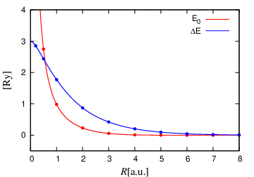
V.2 The ground state and the first excited state
For the lowest state , the behavior of the potential curve at the two asymptotic limits of small and large distances is well known. For the total energy is given by [25, 23, 24]
| (41) |
Choosing the reference point for the energy at zero the behavior at reads [26, 27, 28]
| (42) | |||||
where the first sum represents perturbation theory, the second one is a type of one-instanton contribution etc. As for the lowest state of the negative parity large and small -distance expansions are known as well,
| (43) |
at , while the behavior for is given by Eq. (42) with sign changed from minus to plus in front of the exponential term .
Let us consider the sum of potential curves for and states,
| (44) |
Its corresponding expansions are
| (45) |
at and
| (46) |
at . Now we assume that two-instanton contribution, a large , (and possible higher exponentially-small contributions) can be neglected and construct the analytic approximation for which mimics the two asymptotic limits (45), (46) using Padé approximations with a certain . Concrete fit was made for , where the Padé approximation is of the form ,
| (47) |
with a certain constraints imposed,
| (48) |
After making the fit with (47), we arrive to concrete values of seven free parameters:
| (49) |
It provides 3-4 d.d. for all studied domain . Its free parameters are also in complete agreement in 5-6 s.d. with coefficients in the terms , and of expansion at , see (45) and , and at , in the -expansion (46), see Fig. 4.
In a consistent way, the potential curve for the ground state can be constructed from (47) and (38) by taking
| (50) |
This expression reproduces 3-4 d.d. when comparing with the exact values, see Table 1 and for illustration see Fig. 5. The asymptotic expansions of Eq. (50) are given by
| (51) | |||||
| (52) |
which are in complete agreement with the first three terms at , and with the first three terms in the expansion and two terms in expansion of the pre-factor to for (cf. (41) and (42)).

Similarly, the potential curve for the excited state is restored from (47) and (38) by taking
| (53) |
This expression also reproduces 3-4 d.d. when comparing with the exact values, see Table 2 and for illustration Fig. 6. The asymptotic expansions of Eq. (53) are given by
| (54) | |||||
| (55) |
which are in complete agreement with the first three terms at (cf. (43)), and three terms in expansion and two terms in expansion of the pre-factor to for (cf. (42)).

VI Conclusions
Summarizing we want to state that a simple uniform approximation of the eigenfunctions for the H molecular ion is presented. It allows us to calculate any expectation value or matrix element with guaranteed accuracy. It manifests the approximate solution of the problem of spectra of the H molecular ion. In a quite straightforward way similar approximations can be constructed for general two-center, one-electron system , in particular, for as well as for . It will be done elsewhere.
The key element of the procedure is a straightforward interpolation between the WKB expansion at large distances and perturbation series at small distances for the phase of the wavefunction. Or, in other words, to find with high local accuracy an approximate solution for the corresponding eikonal equation. Separation of variables allowed us to solve this problem constructively. In the case of non-separability of variables the WKB expansion of a solution of the eikonal equation can not be constructed in unified way, since there is a strong dependence of the phase on the way to approach to infinity. However, a reasonable guess on the first growing terms of the WKB expansion seems sufficient to construct the interpolation between large and small distances which leads to highly accuracy results. This program is realized for the problem of the hydrogen atom in a constant magnetic field and will be published elsewhere.
In fact, with unusually high accuracy we are able to approximate the potential curves for the lowest states of positive, and negative, parity in the whole domain of the interproton distances, . Eventually, the interproton interaction potential is described by a superposition of two suitable rational functions with and exponential in weight factors. It is different from the potentials used to approximate internuclear interaction in diatomic molecules (see [29], [30] and [31], and references therein). Analytic form of the approximation of the potential curve gives a chance to calculate the corresponding vibrational states beyond harmonic approximation. Since long ago it was known that at large these potential curves should contain exponentially-small contributions, see e.g. [26, 27, 28], as a result of tunnelling between two degenerate Coulomb wells. Energy difference between potential curves of and states at should be exponentially small, it can not be found in perturbation theory in . We are not aware about any calculations of this difference in instanton calculus. Presence of the second term in generalized Pade approximation, , see (50) and (53), allows us to estimate for the first time the effect of exponentially-small terms to a potential curve at finite . This effect is extremely small at large being at a.u. and giving contribution to 11th s.d. and beyond for a.u. However, it becomes significant at a.u., see Fig. 4.
It is worth mentioning a curious fact that the problem (3) after separation angular dependence possesses the hidden algebra [2]. The differential operator in and is in the universal enveloping algebra of (see e.g. [32]). The spin of the representation is and , respectively. For non-physical, (half)-integer, positive values of and integer ratio the algebras appear in the finite-dimensional representation realized in action on polynomials in , respectively. It explains sometimes observed a mysterious appearance of polynomial solutions for non-physical values of in the problem (3).
Acknowledgements.
The research is supported in part by PAPIIT grant IN108815 and CONACyT grant 166189 (Mexico). H.O.P. is grateful to Université Libre de Bruxelles (Belgium) and Instituto de Ciencias Nucleares, UNAM (Mexico) for a kind hospitality extended to him where a certain stages of the present work were carried out. A.V.T. is grateful to E Shuryak (Stony Brook) for the interest to work and encouragement. A.V.T. gratefully acknowledges support from the Simons Center for Geometry and Physics, Stony Brook University at which some of the research for this paper was performed and where the paper was completed.
Appendix
The easiest way to calculate a deviation of the approximation from the exact eigenfunction is to develop a perturbation theory in framework of the so-called non-linearization procedure [33]: for a chosen approximation a corresponding potential is found with , for which is the exact eigensolution. Then the potential is written in the form , then it is looked for energy and the eigenfunction in the form of power series in the parameter , and , respectively. Eventually, is placed equal to one.
Due to specifics of (1) because of the separation of variables the procedure can be developed for both functions and (see (5)) separately as well as for the separation parameter , while keeping the energy fixed. It can be done for the system of equations (6), (7). As a first step let us transform (6), (7) into the Riccati form by introducing and , respectively,
| (56) |
where the ”potential” , and
| (57) |
where the ”potential” .
Let us choose some , then substitute it to the l.h.s. of (56) and call the result as unperturbed ”potential” putting without loss of generality . The difference between the original and generated is the perturbation, . For a sake of convenience we can insert a parameter in front of and develop the perturbation theory in powers of it. The perturbation theory is also developed for node states where a node position is also looked for the form of power expansion in .
| (58) |
The equation for th correction has a form,
| (59) |
where and
| (60) | |||||
for . Integrating (59) we obtain
| (61) |
where and are obtained in the same way. These are
| (62) |
and
| (63) |
In a similar way by choosing , building the unperturbed ”potential” and putting as zero approximation one can develop perturbation theory in the equation (57)
| (64) |
The equation for th correction has a form similar to (59),
| (65) |
where and
| (66) | |||||
for . Its solution is given by (cf.(61))
| (67) |
where and are obtained in the same way. These are (cf.(62) and (63))
| (68) |
and
| (69) |
In order to realize this perturbation theory a condition of consistency should be imposed
| (70) |
This condition allows us to find the parameter and, hence, the energy and (see (8)).
Sufficient condition for such a perturbation theory to be convergent is to require a perturbation ”potential” to be bounded,
| (71) |
where are constants. Obviously, that the rate of convergence gets faster with smaller values of . It is evident that the perturbations and get bounded if and are smooth functions vanishing at the origin but reproduce exactly the growing terms at tending to infinity in (12), (14), respectively.


References
- [1]
L.D. Landau and E.M. Lifshitz,
Quantum Mechanics, Non-relativistic Theory (Course of Theoretical Physics vol 3), 3rd edn (Oxford:Pergamon Press), 1977 - [2]
A.V. Turbiner and H. Olivares-Pilon,
The H molecular ion: a solution,
J. Phys. B 44 101002 (7 pp) (2011) - [3]
E.A. Hylleraas,
On the Electronic Terms of the Hydrogen Molecule,
Z. Physik 71 739 (1931) - [4]
D.R. Bates, K. Ledsham and A.D. Stewart,
Wave Functions of the Hydrogen Molecular Ion,
Phil. Trans. Roy. Soc. A 246, 215-240 (1953) - [5]
H.E. Montgomery Jr.,
One-electron wavefunctions. Accurate expectation values,
Chem. Phys. Letters, 50, 455-458 (1977) - [6]
D.M. Bishop and L.M. Cheung,
Moment functions (including static dipole polarisabilities) and radiative corrections for H,
J. Phys. B 11, 3133-3144 (1978) - [7]
V.I. Korobov,
Coulomb variational bound state problem: variational calculation of nonrelativistic energies,
Phys. Rev. A 61 064503 (2000) - [8]
M.P. Strand and W.P. Reinhardt,
Semiclassical quantization of the low lying electronic states of H,
J. Chem. Phys. 70, 3812-3827 (1979) - [9]
A.V. Turbiner,
Anharmonic oscillator and double-well potential: approximating eigenfunctions,
Lett. Math. Phys. 74, 169-180 (2005) - [10]
A.V. Turbiner,
Double well potential: perturbation theory, tunneling, WKB (beyond instantons),
Int. J. Mod. Phys. A 25, 647-658 (2010) - [11]
H.A. Erikson and E.L. Hill,
A note about one-electron states of diatomic molecules,
Phys. Rev. 76, 29 (1949) - [12]
C.A. Coulson and A. Joseph,
A constant of motion for the two-centre Kepler problem,
Internat. J. Quant. Chem. 1, 337-347 (1967) - [13]
M. Vincke and D. Baye,
Hydrogen molecular ion in an aligned strong magnetic field by the Lagrange-mesh method,
J. Phys. B 39, 2605-2618 (2006) - [14]
D. Baye,
The Lagrange-mesh method,
Phys. Repts. 565, 1-107 (2015) - [15]
D.M. Bishop,
Ab Initio Calculations of Harmonic Force Constants. III. An Exact Calculation of the H Force Constant,
J. Chem. Phys 53 1541-1542 (1970) - [16]
J.M. Peek,
Discrete Vibrational States Due Only to Long-Range Forces: State of H,
J. Chem. Phys 50 4595-4596 (1969) - [17]
M.M. Madsen and J.M. Peek,
Eigenparameters for the lowest twenty electronic states of the Hydrogen molecular ion,
Atomic Data, 2, 171-204 (1971) - [18]
T.C. Scott, M. Aubert-Frecon and J. Grotendorst,
New Approach for the Electronic Energies of the Hydrogen Molecular Ion,
J. Chem. Phys. 324, 323-338 (2006) - [19]
D.R. Bates, R.T.S. Darling, S.C. Hawe and A.L. Stewart,
Properties of the Hydrogen Molecular Ion III: Oscillator Strengths of the , and Transitions ,
Proc. Phys. Soc. A 66, 1124 (1953) - [20]
D.R. Bates, R.T.S. Darling, S.C. Hawe and A.L. Stewart,
Properties of the Hydrogen Molecular Ion IV: Oscillator Strengths of the Transitions Connecting the Lowest Even and Lowest Odd -States with Higher -States,
Proc. Phys. Soc. A 67, 533 (1954) - [21]
Ts. Tsogbayar and Ts. Banzragch,
The Oscillator Strengths of H, 1-2, 1-2,
ArXiv:physics.atom-ph/1007.4354v1 (2010) - [22]
A. Dalgarno and R. McCarroll,
Properties of the Hydrogen Molecular Ion VII: Magnetic Dipole Oscillator Strengths of the Transition,
Proc. Phys. Soc. A 70, 501 (1957) - [23]
W. Byers Brown and E. Steiner,
On the Electronic Energy of a One-Electron Diatomic Molecule near the United Atom,
J. Chem. Physics 44, 3934-3940 (1966) - [24]
M. Klaus,
On H for small internuclear separation,
J. Phys. A: Math, Gen. 16, 2709-2720 (1983) - [25]
W.B. Brown,
Interatomic Forces at Very Short Range,
Discussions Faraday Soc. 40 140-149, (1965) - [26]
A.A. Ovchinkikov, and A.D. Sukhanov,
Dokl.Akad.Nauk, SSSR, 157, 1092-1095 (1964),
Soc.Phys.-Dokl. 9, 685-687 (1965)(English translation) - [27]
R.J. Damburg and R.Kh. Propin,
On asymptotic expansions of electronic terms of the molecular ion H,
J. Phys. B. (Proc Phys. Soc.) 1 , 4, 681-691 (1968) - [28]
J. Cizek et al.,
expansion for : Calculation of exponentially small terms and asymptotics,
Phys. Rev. A 33, 12 - 54 (1986) - [29] C.L. Beckel and P.R. Findley, Rational fraction representation to diatomic vibrational potentials. Application to ground state J. Chem. Phys 73, 3517 - 3518 (1980)
- [30]
S.A. Sonnleitner and C.L. Beckel,
Rational fraction representation of diatomic vibrational
potentials. IV. The van der Waals state of H,
J. Chem. Phys 73, 5404 - 5405 (1980) - [31]
S. Warnicke, K.T. Tang, and J P Toennies,
Communication: Simple full range analytic potential for H2, H-He, He2,
J. Chem. Phys 142 131102 (2015) - [32]
A.V. Turbiner,
Quasi-Exactly-Solvable Problems and the Algebra,
Comm. Math. Phys. 118, 467-474 (1988) - [33]
A.V. Turbiner,
On Perturbation Theory and Variational Methods in Quantum
Mechanics,
ZhETF 79, 1719 (1980);
Soviet Phys.-JETP 52, 868 (1980) (English Translation);
The Problem of Spectra in Quantum Mechanics and the ‘Non-Linearization’ Procedure,
Usp. Fiz. Nauk. 144, 35 (1984);
Sov. Phys. – Uspekhi 27, 668 (1984) (English Translation)