Motion planning and control of a planar polygonal linkageThanks: The authors acknowledge useful discussions with George Khimshiashvili and hospitality of CIRM, Luminy, where this research was completed in framework of ”Research in Pairs” program in January of 2014. The first author was also supported by RFBR grant 15-01-02021. We are also grateful to Troy Baker for a number of English corrections.

Gaiane Panina Address: Institute for Informatics and Automation, St. Petersburg, Russia, Saint-Petersburg State University, St. Petersburg, Russia. and Dirk Siersma Address: University of Utrecht, Mathematisch Instituut, Utrecht, The Netherlands.

Abstract.

For a polygonal linkage, we produce a fast navigation algorithm on its configuration space. The basic idea is to approximate the configuration space by the vertex-edge graph of its cell decomposition discovered by the first author. The algorithm has three aspects: (1) the number of navigation steps does not exceed 15 (independent of the linkage), (2) each step is a disguised flex of a quadrilateral from one triangular configuration to another, which is a well understood type of flex, and (3) each step can be performed explicitly by adding some extra bars and obtaining a mechanism with one degree of freedom.

1. Introduction

In the paper we work with a polygonal linkage (equivalently, with a flexible polygon), that is, with a collection of rigid bars connected consecutively in a closed chain. We allow any number of edges and any lengths assignment, (under a necessary assumption of the triangle inequality, which guarantees the closing possibility). The flexible polygon lives in the plane and admits different shapes, with allowed self-intersections. Taken together, all the shapes form the moduli space of the linkage. In the paper, we produce a motion planning algorithm (equivalently, a navigation algorithm) which explicitly reconfigures one shape to another via some continuous motion. In the language of the moduli space this means that we present a path leading from one prescribed point to another. We not only indicate the path, but also present a way of forcing the linkage to follow the path.

Although the problem does not seem very complicated (since the more edges we have, the more degrees of freedom we have), the navigation is not an easy issue because of the (possible) topological complexity of the moduli space.

There exists (see [5]) an $O(n)$ algorithm, where each step is a line-tracking motion. That is, during each step, the entire polygon except for some pentagonal subchain is frozen, only the subchain flexes in such a way that one of its vertices moves along a straight line.

Our reconfiguring algorithm is based on a stratification of the moduli space into a cell complex, introduced in [7]. More precisely, we treat the one-skeleton of the complex as an appropriate approximation of the moduli space. In other words, we have an embedded graph, and we mostly navigate along the graph. The navigation goes as follows: from a given configuration of the linkage, we first reach an appropriate vertex of the graph, then navigate along the graph until we are close to the target configuration, and next, we pass to the target configuration. There are three important aspects about the algorithm:

(1)

The number of steps (i.e., the number of edges of the connecting path) never exceeds 15. That is, we have a finite time algorithm (rather than $n$ or even $log\ n$ complexity).
(2)

However, finding each of the 15 designated configurations requires a linear time complexity algorithm.
(3)

Each of the steps (that is, going along an edge of the graph) is a disguised flex of a quadrilateral polygonal linkage, which is both simple and well-understood.
(4)

Each of the steps can be performed explicitly by adding some extra bars and obtaining a mechanism with one degree of freedom, see Section 4.

The paper is organized as follows. Section 2 gives precise definitions and explains the cell structure on the configuration space. We also present introductory examples and give a formula for the number of vertices of the vertex-edge graph of the complex $\Gamma$ . Section 3 explains the navigation on the graph. We show that a vertex-to-vertex navigation requires at most 15 steps.

Our next goal is to realize the prescribed motions. We work under assumption that we have a full control of convex configurations, that is, we know how to reconfigure one convex configuration to another. There are different approaches how to do this: by using Coulomb potential, as in [12], by mechanically controlling the angles, in the way described in [1], or in some other way, not to be discussed in the paper. However we stress that for navigating over edges of the graph, it suffices to control just quadrilaterals, which is a much easier task and well understood in all respects.

Navigation from an arbitrary point of the moduli space to a vertex requires one more step: we need to connect the starting point to the graph. Two different ways of doing this are described in Section 4.

The results presented in this paper arose as a natural continuation of the research on Morse functions on moduli spaces of polygonal linkages started in [10], [11], and [12]. Several approaches to navigation and control of mechanical linkages have previously been discussed, in particular, in [8], [9], [10] and [12].

2. Moduli spaces of planar polygonal linkages

We start by a short review of some results on polygonal linkages and their moduli spaces.

A polygonal $n$ -linkage is a sequence of positive numbers $L=(l_{1},\dots,l_{n})$ . It should be interpreted as a collection of rigid bars of lengths $l_{i}$ joined consecutively in a chain by revolving joints. In the literature, it is sometimes called a closed chain.

We assume that the closing condition holds: the length of each bar is less than the total length of the rest.

A configuration of $L$ in the Euclidean plane $\mathbb{R}^{2}$ is a sequence of points $R=(p_{1},\dots,p_{n}),\ p_{i}\in\mathbb{R}^{2}$ with $l_{i}=|p_{i},p_{i+1}|$ , and $l_{n}=|p_{n},p_{1}|$ .

Definition 2.1.

The set $M(L)$ of all configurations modulo orientation preserving isometries of $\mathbb{R}^{2}$ is the moduli space, or the configuration space, of the linkage $L$ .

Definition 2.2.

Equivalently, $M(L)$ can be defined as the quotient space

M(L)=\{(u_{1},...,u_{n})\in(S^{1})^{n}:\sum_{i=1}^{n}l_{i}u_{i}=0\}/SO(3).

Now let us treat the lengths $l_{i}$ as variables. Each $n$ -tuple of positive numbers gives us a polygonal linkage which comes together with its configuration space. The hyperplanes

\sum_{i\in J}l_{i}=\sum_{i\notin J}l_{i},

where $J$ ranges over all subsets of $[n]$ , are called walls. (Here and in the sequel, $[n]$ denotes the set $\{1,...,n\}$ .) The walls decompose $\mathbb{R}_{>0}^{n}$ into a collection of chambers.

Here is a (far from complete) summary of facts about $M(L)$ :

•

If no configuration of $L$ fits a straight line, or, equivalently, $L$ does not lie on a wall, then $M(L)$ is a smooth $(n-3)$ -dimensional manifold. In this case, the linkage is called generic [4]. Throughout the paper we consider only generic linkages.
•

The topological type of the moduli space $M(L)$ depends only on the chamber containing $L$ [4].
•

$M(L)$ admits a structure of a regular cell complex [7]. The combinatorics is very much related (but not identical) to the combinatorics of the permutohedron. The construction is explained later in this section.
•

Definition 2.2 implies that the moduli space $M(L)$ , as well as the cell structure, does not depend on the permutation of the edgelengths $l_{i}$ . More precisely, for any permutation $\sigma\in S_{n}$ , there exists a canonical isomorphism between $M(L)$ and $M(\sigma(L))$ , which maintains the cell structures.

Definition 2.3.

A set $I\subset[n]$ is called long, if

|I|=\sum_{i\in I}l_{i}>\sum_{i\notin I}l_{i}.

Equivalently, for a long set $I$ ,

|I|>\frac{|L|}{2}.

Otherwise, $I$ is called short.

Note that because of the genericity assumption, we never have $|I|=\frac{|L|}{2}.$

We stress that the manifold $M(L)$ (considered either as a topological manifold, or as a cell complex) is uniquely defined by the collection of short subsets of $[n]$ .

Example 2.4.

Assume that for an $n$ -linkage $L$ , we have the following:

\forall\ i=1,2,...,(n-1),\hbox{ the set }\{n,i\}\hbox{ is long.}

Loosely speaking, we have ”one long edge”. Such a linkage we call an $n$ -bow; its moduli space is a sphere (see [2]).

Definition 2.5.

A partition of the set $\{l_{1},\dots,l_{n}\}$ is called admissible if all the parts are non-empty and short.

Instead of partitions of $\{l_{1},\dots,l_{n}\}$ we shall speak of partitions of the set $[n]$ , keeping in mind the lengths $l_{i}$ .

Description of the cell complex

Now we sketch the cell complex structure on the moduli space $M(L)$ , referring the reader to [7] for even more details and all the proofs.

The cell structure comes from the following labeling of configurations. Given a configuration $P$ of $L$ without parallel edges, there exists a unique convex polygon $Conv(P)$ which we call the convexification of $P$ such that

(1)

The edges of $P$ are in one-to-one correspondence with the edges of $Conv(P)$ . The bijection preserves the directions of the vectors.
(2)

The edges of $Conv(P)$ are oriented in the counterclockwise direction with respect to $Conv(P)$ .

In other words, the edges of $Conv(P)$ are the edges of $P$ ordered by the slope (see Fig. 1). Obviously, $Conv(P)\in M(\lambda L)$ for some permutation $\lambda\in S_{n}$ . The permutation is defined up to some power of the cyclic permutation $(2,3,4,...,n,1)$ , and hence can be considered as a cyclic ordering on the set $[n]$ .

Refer to caption — Figure 1. Labeling of a polygon with no parallel edges

Our construction assigns to $P$ the label $\lambda$ , considered as a cyclic ordering on the set $[n]$ . Equivalently, a label of a configuration without parallel edges is a cyclically ordered partition of the set $[n]$ into $n$ singletons. Figure 1 gives an example.

If $P$ has parallel edges, a permutation which makes $P$ convex is not unique, since there is no ordering on the set of parallel edges. The label assigned to $P$ is a cyclically ordered partition of the set $[n]$ , where parallel edges belong to the same subset in the partition. Fig. 2 gives an example.

An obvious observation is that all labels are admissible partitions.

A remark on notation. We write a cyclically ordered partition as a (linearly ordered) string of sets, keeping in mind that the string is closed.

We stress once again that there is no ordering inside a set, that is, two labels are equal when they differ only by permutations of the elements inside the sets. For instance,

(\{1\}\{3\}\{4256\})\neq(\{3\}\{1\}\{4256\})=(\{3\}\{1\}\{2456\}).

Definition 2.6.

Two points from $M(L)$ (that is, two configurations) are equivalent if they have the same label. Equivalence classes of $M(L)$ are the open cells. The closure of an open cell in $M(L)$ is called a closed cell. For a cell $C$ , either closed or open, its label $\lambda(C)$ is defined as the label of any interior point.

With this labeling, the following theorem is valid.

Theorem 2.7.

[7] The above described collection of open cells yields a structure of a regular CW-complex $\mathcal{K}(L)$ on the $(n-3)$ -dimensional manifold $M(L)$ . Its complete combinatorial description reads as follows:

(1)

$k$ -cells of the complex $\mathcal{K}(L)$ are labeled by cyclically ordered admissible partitions of the set $[n]$ into $(k+3)$ non-empty parts.
(2)

In particular, the facets of the complex (that is, the cells of maximal dimension) are labeled by cyclic orderings of the set $[n]$ .
(3)

A closed cell $C$ belongs to the boundary of some other closed cell $C^{\prime}$ iff the partition $\lambda(C^{\prime})$ is finer than $\lambda(C)$ .
(4)

The complex is regular, which means that each $k$ -cell is attached to the $(k-1)$ -skeleton by an injective mapping. All closed cells are ball-homeomorphic. ∎

Example 2.8.

The vertex labeled by

(\{1,2,5,6\},\{3,4\},\{7,8\})

and the vertex labeled by

(\{1,2\},\{3,4,5,6\},\{7,8\})

are connected by an edge labeled by

(\{1,2\},\{5,6\},\{3,4\},\{7,8\}).

Example 2.9.

Let $n=4;\ \ l_{1}=l_{2}=l_{3}=1,\ l_{4}=1/2.$ The moduli space $M(L)$ is known to be a disjoint union of two circles (see [2]). The cell complex $\mathcal{K}(L)$ is depicted in Fig. 3.

Example 2.10.

Assume that for a $4$ -linkage $L$ , the sets $\{2,3\}$ , $\{4,3\}$ , and $\{2,4\}$ are short. An example of such a length assignment is

l_{4}=l_{2}=l_{3}=1,\ l_{1}=2.5.

The moduli space $M(L)$ is homeomorphic to a circle. The cell complex is combinatorially a hexagon, that is, there are six vertices connected by six edges into a circle. The (cyclic) order of the labels of the six vertices is:

(\{1\}\{2,3\}\{4\})

(\{1\}\{2\}\{4,3\})

(\{1\}\{2,4\}\{3\})

(\{1\}\{4\}\{2,3\})

(\{1\}\{4,3\}\{2\})

(\{1\}\{3\}\{4,2\}).

Example 2.11.

For the equilateral pentagonal linkage $L=(1,1,1,1,1)$ , the complex $\mathcal{K}(L)$ has $30$ vertices, $60$ edges, and $24$ pentagonal $2$ -cells. Each vertex is incident to exactly four edges.

In the paper we shall make use of the vertex-edge graph $\Gamma$ of the cell complex, that is, we take into account only zero- and one-dimensional cells. We treat it as a (combinatorial) graph, also keeping in mind its embedding in the $M(L)$ . This allows us to view the graph $\Gamma$ as a discrete approximation of the moduli space.

Combinatorics of the vertex-edge graph

Assume that a linkage $L$ is fixed. As a particular case of Theorem 2.7, vertices of $\Gamma$ are labeled by cyclically ordered partitions of $[n]$ into three non-empty short sets, and the edges are labeled by cyclically ordered partition of $[n]$ into four non-empty short sets. Two vertices labeled by $\lambda$ and $\lambda^{\prime}$ are joined by an edge whenever the label $\lambda$ can be obtained from $\lambda^{\prime}$ by shifting some amount of entries from one set to another, as in Example 2.8.

Embedding of the vertex-edge graph

Now we describe a way of retrieving the vertex-edge graph $\Gamma$ from the labels.

Algorithm 1.

Retrieving a vertex (viewed as a polygon) by its label.

Given a label $\lambda=(I,J,K)$ , it corresponds to a unique point $P\in M(L)$ , that is, to some configuration of $L$ . The polygon $P$ can be constructed as follows.

(1)

Take a positively oriented triangle with edgelengths

$\sum_{I}l_{i},\ \sum_{J}l_{i},\hbox{ and }\sum_{K}l_{i}.$
(2)

We assume that each edge is composed of segments $l_{i}$ . For instance, we decompose the first edge into segments of lengths $\{l_{i}\}_{i\in I}.$ Their order does not matter.
(3)

Now take all the edges apart, keeping their directions, and rearrange them according to the ordering $1,2,...,n$ . We get a closed polygonal chain $P$ , see Figure 4.

Taken together, all labels give all configurations that have exactly 3 directions of the edges. They form the vertex set of the embedded graph $\Gamma(L)$ .

Now let us explain how the edges are embedded.

Algorithm 2.

Retrieving an edge by its label

Given a label $\lambda=(I,J,K,N)$ , it labels an embedded edge of $\Gamma(L)$ , that is, a one-parametric family of configurations. They are retrieved as follows.

(1)

Take a positively oriented convex quadrilateral with consecutive edgelengths

$\sum_{I}l_{i},\ \sum_{J}l_{i}\ \sum_{K}l_{i},\hbox{ and }\sum_{N}l_{i}.$

The set of such quadrilaterals forms a path in $M(L)$ going from one triangle to another, see Figure 5.
(2)

As in Algorithm 1, decompose each edge into (short) edges $l_{i}$ .
(3)

Exactly as in algorithm 1, take all the edges apart, keeping their directions, and rearrange them according to the ordering $1,2,...,n$ . This gives a one-parametric family of closed polygonal chains.

In other words, each embedded edge of the graph $\Gamma(L)$ corresponds to a flex of some quadrilateral, which connects two triangular configurations. Such a flex can be performed by compressing one of the diagonals.

Lemma 2.12.

(1)

The number of vertices of $\Gamma(L)$ equals

$\sum_{k=1}^{n}N_{k}2^{n-k}-2\cdot 3^{n-1}+2^{n},$

where $N_{k}$ is the number of short $k$ -sets.
(2)

For the $n$ -bow, $\Gamma(L)$ has the minimal possible number of vertices among all $n$ -linkages. In this case, it equals $2^{n-1}-2$ .

Proof. We start with the bow linkage (see Example 2.4), and then change $L\in\mathbb{R}^{n}$ continuously. From the chamber that corresponds to the bow, we can reach any other chamber by crossing walls. As follows from the construction of the cell complex, the graph $\Gamma$ changes only when $L$ crosses a wall. ”Crossing a wall” means that exactly one short $k$ -set $I$ becomes long, and exactly one long $(n-k)$ -set $\overline{I}$ becomes short, where the number $k$ depends on the wall. Observe that any proper subset of $\overline{I}$ is short both before and after crossing a wall. A vertex is eliminated whenever its label contains $I$ . A vertex arises whenever its label contains $\overline{I}$ . This means that after crossing a wall, the number of vertices changes by adding $(2^{k}-2)-(2^{n-k}-2)=2^{k}-2^{n-k}$ .

Therefore,

|Vert(\Gamma)|=\sum_{k=1}^{n}N_{k}2^{n-k}+X_{n},

where $X_{n}$ depends solely on $n$ . Our second observation is that for a bow linkage, labels of the vertices are as follows:

(I,\ [n-1]\setminus{I},\{n\}),

where $I$ is any proper non-empty subset of $[n-1]$ . Therefore,

|Vert(\Gamma(n\hbox{-bow}))|=2^{n-1}-2.

This is the base case of an induction.

For the $n$ -bow,

N_{k}=\left\{\begin{array}[]{ll}0=C_{n-1}^{0}-1,&\hbox{if }k=0;\\ n=C_{n-1}^{1}+1,&\hbox{if }k=1;\\ 0=C_{n-1}^{n-1}-1,&\hbox{if }k=n-1\\ C_{n-1}^{k},&\hbox{ otherwise.}\end{array}\right.

2^{n-1}-2=\sum_{k=0}^{n}C_{n-1}^{k}2^{n-k}+2^{n-1}-2^{n}-2+X_{n}

X_{n}=2^{n}-2\cdot 3^{n-1},

which yields the final formula.∎

As we see, the number of vertices of the graph $\Gamma$ depends exponentially on $n$ . However, the valence of the vertices also depends on $n$ exponentially, so one can expect a small diameter (in the graph-theoretic sense, that is, the maximal length of the shortest path between two vertices), and a fast navigating algorithm.

Lemma 2.13.

A vertex of the graph $\Gamma$ labeled by $(I,J,K)$ has exactly

2^{i}+2^{j}+2^{k}-6

incident edges, where $i,\ j,$ and $k$ are the numbers of elements in $I,\ J,$ and $K$ respectively.∎

3. Motion planning on the graph $\Gamma(L)$

Here we describe a finite-step algorithm of motion planning (or, equivalently, navigation) from an arbitrary vertex of $\Gamma(L)$ to an arbitrary target vertex.

A path means a graph-theoretical path, that is, a consecutive collection of edges. By its length, or the number of steps we mean just the number of edges in the path.

We start with an example demonstrating that the proposed navigation works quickly.

Algorithm 3.

(Navigation for the bow linkage) For an $n$ -bow linkage with $n>3$ , any two vertices of $\Gamma(L)$ are connected by a path whose length is at most 3. The path is explicitly described as follows.

(1)

We start with a vertex labeled by

$(I,J,\{n\}).$

We may assume that the target vertex is labeled by

$(\{1,2,...,k\},\{k+1,k+2,...,n-1\},\{n\}).$

If this is not the case, we can renumber the edges of the linkage: we know that in view of Definition 2.2, renumbering maintains the manifold $M(L)$ and the cell structure.
(2)
If $|J|>1$ ,
1. (a)
  
  If $1\in I$ , then go to the step (b). If not, shift the entry $1$ to the set $I$ and go to step (b).
2. (b)
  
  Shift the set $I\setminus\{1\}$ to the set $J$ . We arrive at the vertex labeled by
  
  $(\{1\},\{2,3,...,n-1\},\{n\}).$
3. (c)
  
  Shift the set $\{2,3,...,k\}$ to the first set and get the target vertex.∎
(3)
If $|J|=1$ , then $|I|>1$ . We act similarly to the case (2), exchanging the roles of $I$ and $J$ . Namely:
1. (a)
  
  If $(k+1)\in J$ , then go to the step (b). If not, shift the entry $(k+1)$ to the set $J$ and go to step (b).
2. (b)
  
  Shift the set $J\setminus\{k+1\}$ to the set $I$ . We arrive at the vertex labeled by
  
  $(\{1,2,...,k,k+2,...\},\{k+1\},\{n\}).$
3. (c)
  
  Shift the set $\{k+2,k+3,...,n-1\}$ to the second set.∎

Now we pass from a bow to arbitrary linkages. We first produce an auxiliary algorithm which turns polygons inside out, that is, connects a configuration with its mirror image by a path.

Algorithm 4.

(Turning a pentagon inside out) Assume that a $5$ -linkage $L$ satisfies the following conditions:

(1)

The set $\{1,2\}$ is long.
(2)

The set $\{1,5\}$ is long.
(3)

$\forall\ i\neq 1,\ j\neq 1,$ the set $\{i,j\}$ is short.

Then there exists a 4-steps path which turns the configuration $(\{4,5\}\{1\}\{2,3\})$ inside out. Here it is:

(\{4,5\}\{1\}\{2,3\})

(\{4,5,3\}\{1\}\{2\})

(\{4,3\}\{1\}\{2,5\})

(\{4,3,2\}\{1\}\{5\})

(\{3,2\}\{1\}\{4,5\})

Algorithm 5.

(Turning an arbitrary polygon inside out) Assume that a linkage $L$ is fixed.

(1)

If the configuration space $M(L)$ is connected, then from each vertex $V$ labeled by $(I,J,K)$ there are at most six steps to its mirror image $(K,J,I)=(J,I,K)$ .
(2)

If the $M(L)$ is disconnected, then the vertex $(I,J,K)$ and its mirror image $(J,I,K)$ lie in different connected components, and no connecting path exists.

The idea is to imitate a pentagon which satisfies the three conditions of the Algorithm 4 by freezing some of the entries in $L$ . Here and in the sequel, ”freezing” means putting the entries into one separate set and after that, manipulating with the set as with a single entry.

Assume that $l_{1}\geq l_{k}\geq l_{m}$ are the longest edges of $L$ . It is known from [4] that $M(L)$ is connected if and only if

l_{k}+l_{m}<\frac{|L|}{2}.

Our starting point is a vertex labeled by $(I,J,K)$ , where $1\in J$ . We can assume this, since $(I,J,K)=(J,K,I)=(K,I,J).$ Since we can apply renumbering of the edges, we also can assume that the entries are as follows:

(I,J,K)=(\{r+1,r+2,...,p\}\{p+1,p+2,...,n,1,2,...,q\}\{q+1,q+2,...,r\}).

Steps 1–2: necessary preparations before freezing: pushing entries to the central set.

Maintaining the ordering, we shift to the middle set as many entries from the first and the last sets as is possible. In more detail, we first decide what entries should be shifted from $I$ , and what entries should be shifted from $K$ . After the decision is done, we make two shifts, which means two steps. The choice is not uniquely defined; however, any choice will suffice. The result we denote by

(I\setminus I^{\prime},J\cup I^{\prime}\cup K^{\prime},K\setminus K^{\prime}),

for which we keep the same notation:

(I\setminus I^{\prime},J\cup I^{\prime}\cup K^{\prime},K\setminus K^{\prime})=

=(\{r+1,r+2,...,p\}\{p+1,p+2,...,n,1,2,...,q\}\{q+1,q+2,...,r\}).

Steps 3–6: freeze the linkage either to a quadrilateral or to a pentagon, and then turn it inside out. On this step we work under assumption that $M(L)$ is connected. A necessary observation is that now the set $\{p,q+1\}$ is short. Indeed,

l_{p}+l_{q+1}\leq l_{k}+l_{m}<\frac{|L|}{2}.

Therefore the set

A=\{q+2,q+3,..,r,r+1,...,p-2,p-1\}

is not empty.

Now the algorithm splits depending on the number of entries in $A$ which equals $(p-1)-(q+2)+1=p-q-2$ .

(1)

Assume that $p-q-2=1$ , which means that $A$ is a one-element set. Then we freeze the set $\{p+1,p+2,...,n,1,2,...,q\}.$ After renumbering

$4:=\{p\},\ 1:=\{p+1,p+2,...,n,1,2,...,q\},$

$\ 2:=\{q+1\},\hbox{ and }3:=A,$

we arrive at a quadrilateral from Example 2.10 which can be turned inside out in three steps.
(2)

Assume that $p-q-2>1$ . We divide the set $A$ into two non-empty subsets and freeze the two subsets. We also freeze the set $\{p+1,p+2,...,n,1,2,...,q\}.$ That is, for instance, we freeze the following three sets of entries:

$\{r+1,r+2,...,p-1\},\ \{p+1,p+2,...,n,1,2,...,q\},\ \hbox{ and }\{q+2,...,r\}.$

After renumbering

$4:=\{r+1,r+2,...,p-1\},\ 5:=\{p\},\ 1:=\{p+1,p+2,...,n,1,2,...,q\},$

$\ 2:=\{q+1\},\hbox{ and }3:=\{q+2,...,r\},$

we arrive at a pentagon which satisfies the properties from the Algorithm 4, and therefore can be turned inside out in four steps.

Steps 7–8. Pushing entries from the central set. We have arrived at a vertex labeled by

(K\setminus K^{\prime},J\cup I^{\prime}\cup K^{\prime},I\setminus I^{\prime}).

In two steps we get to $(K,J,I)$ . These steps are reverse to steps 1–2.

Algorithm 6.

For any $n$ -linkage $L$ , and any two vertices $V$ and $V^{\prime}$ of the graph $\Gamma(L)$ , the vertex $V$ is connected either to $V^{\prime}$ or to the mirror image of $V^{\prime}$ by a path whose length is at most 7. The path is explicitly described as follows. Assume that $l_{1}$ is the longest edge, and that the target vertex $V^{\prime}$ is labeled by

(\{1,2,...,k\},\{k+1,k+2,...,m\},\{m+1,m+2,...,n\}).

(1)
In two steps we get from $V$ to a vertex labeled by

$(I,\{1\},J)$

for some $I$ and $J$ . This is always possible:
1. (a)
  
  Assume that $V$ is labeled by $(A,B,C)$ , and $1\in B$ . Start shifting the entries from $B\setminus\{1\}$ to the set $C$ . We shift as many entries as possible, that is, we think of shifting them one by one until $C$ is short, and stop if no other entry can be added to $C$ without making it long. The order in which we treat the entries does not matter. However, we should shift all the entries by one step, that is, first decide what entries are to be shifted, and next, shift them as one subset.
2. (b)
  
  Shift the rest of $B\setminus\{1\}$ to the set $A$ .
(2)

If one of the sets $I$ or $J$ contains two consecutive entries, we can freeze them. We freeze all possible pairs of consecutive entries and renumber the edges (preserving the ordering), which gives us a linkage with a smaller number of edges.

In any case we have a vertex labeled either by

$(\{3,5,7,...\},\{1\},\{2,4,6,8,...\}),$

or by the symmetric image

$(\{2,4,6,8,...\},\{1\},\{3,5,7,...\}).$
(3)

Pull $2,3,4,...,s$ and $3,5,7,...,s\pm 1$ to the middle set for the largest $s$ which is possible. (This requires 2 steps more). Thus we arrive either at the vertex

$(\{s+1,s+3,...\},\{1,2,3,4,...,s\},\{s+2,s+4,...\}),$

or at its symmetric image

$(\{s+2,s+4,...\},\{1,2,3,4,...,s\},(\{s+1,s+3,...\}).$

So the first entry that we cannot shift to the middle set is $s+1$ .
(4)

Shift $s+3,s+5,...$ to the third set. It is possible because
$\{1,2,3,4,...,s,s+1\}$ is long. We arrive either at

$(\{s+1\},\{1,2,3,...,s\},\{s+2,s+3,....,n\})=$

$=(\{s+1\},\{s,s-1,...,2,1\},\{n,n-1,...,s+2,s+3\}),$

or at the symmetric image. Now we have either clockwise or counterclockwise ordering on the entries.
(5)

There are two steps either to the target, or to the mirror image of the target vertex. ∎

Combining the two above algorithms, we immediately have the theorem:

Theorem 3.1.

(1)

For any $n$ -linkage $L$ with a connected moduli space, any two vertices $V$ and $V$ ’ of the graph $\Gamma(L)$ are connected by a path whose length is at most 15.
(2)

For any $n$ -linkage $L$ with a disconnected moduli space, and any two vertices $V$ and $V$ ’ of the graph $\Gamma(L)$ lying in the same connected component, $V$ and $V$ ’ are connected by a path whose length is at most 7.

The path is constructed explicitly using the above algorithms. That is we have the following algorithm:

Algorithm A

(1)

Starting with a vertex $V$ , follow Algorithm 6. It may bring us to the target point, and then we are done.
(2)

If on the first step we get the mirror image of the target point, turn it inside out via Algorithm 5. ∎

Now we exemplify the steps of the algorithm for one particular heptagonal configuration.

Example 3.2.

Assume we have a heptagonal linkage with edge lengths

l_{1}=10,\ l_{2}=1,\ l_{3}=9,\ l_{4}=4,\ l_{5}=9,\ l_{6}=2,\ \hbox{ and }l_{7}=4.

Assume that our starting point is $V_{1}=(\{3,6\}\{1,4,7\}\{2,5\})$ , and that the target vertex is $V^{\prime}=(\{5,6,7\}\{1,2\}\{3,4\})$ . Then Algorithm A runs as is described below and as is depicted in Figure 6.

(1)

The starting point is the vertex of the graph

$V_{1}=(\{3,6\}\{1,4,7\}\{2,5\}).$

According to Algorithm 6, we go to the point

$V_{2}=(\{3,6\}\{1,4\}\{2,5,7\}),$

which is connected with $V_{1}$ by an edge labeled by $(\{3,6\}\{1,4\}\{7\}\{2,5\})$ . Next come the vertices

$V_{3}=(\{3,4,6\}\{1\}\{2,5,7\})$

$\hbox{ and }V_{4}=(\{3,4,6\}\{1,2\}\{5,7\}).$

Then comes the vertex

$V_{5}=(\{3,4\}\{1,2\}\{5,7,6\})=(\{4,3\}\{2,1\}\{7,6,5\}),$

which is the mirror image of the target point.

Now we start turning the configuration inside out, as is prescribed in Algorithm 5.
(2)

The next point is

$V_{6}=(\{3,4\}\{1,2,7,6\}\{5\}).$

After freezing the middle set, we get a triangular configuration of a quadrilateral to be turned inside out in three steps:

$V_{7}=(\{3\}\{1,2,7,6\}\{5,4\}),$

$V_{8}=(\{5,3\}\{1,2,7,6\}\{4\}),$

$V_{9}=(\{5\}\{1,2,7,6\}\{3,4\})=(\{5\}\{6,7,1,2\}\{3,4\}).$

One more edge brings us to the target point

$V_{10}=(\{5,6,7\}\{1,2\}\{3,4\})=V^{\prime}.$

4. Navigation and control on the moduli space

Here we describe a finite-step algorithm of navigation from an arbitrary point (which is not necessarily a vertex of $\Gamma(L)$ ) of the moduli space $M(L)$ to an arbitrary target point.

We work under assumption that we can somehow control the shape of a convex configuration. As an example, we can use the result of [1], where it is shown that a convex polygon can be moved into any other convex polygon with the same counterclockwise sequence of edge lengths in such a way that each angle changes monotonically.

At the same time, we explain how to realize the flex explicitly. As in the previous section, we assume that $l_{1}$ is the biggest edgelength.

Algorithm B

(1)

Given a starting configuration $S$ and a target configuration $T$ , we take the $(n-3)$ -cells of the complex $\mathcal{K}(L)$ containing $S$ and $T$ . The cells may be not unique, if this is the case, choose $S$ and $T$ to be any of them. We choose $V_{S}=(I,\{1\},J),$ and $V_{T}$ to be some vertices of these two cells. Starting from now, we keep in mind Algorithm A applied for the vertices $V_{S}$ and $V_{T}$ .
(2)

We navigate from $S$ to $V_{S}=(I,\{1\},J)$ . In particular, this means that we spare one step compared to Algorithm 6.

We realize both $P$ and the convexification $Conv(P)$ as two bar-and-joint mechanisms. By construction, there is a natural bijection between edges of the two polygons, and the corresponding edges are parallel. For each pair of parallel edges (one edge from $P$ , and the other one from $Conv(P)$ ), we plug in a pair of parallelograms as is shown in Figure 7.

Figure 7. Connecting parallelograms

To prevent turning inside out, we add one extra edge inside each of the parallelograms (here we follow [3]).

Each (convex) flex of $Conv(P)$ uniquely induces a flex of $P$ in such a way that the first polygon remains the convexification of the second one. Therefore, the task is to bring the convex polygon $Conv(P)$ to a triangular configuration. By assumption, we can control $Conv(P)$ , and therefore, we have a controlled way of bringing $P$ to the vertex $(I,\{1\},J).$
(3)

On this step, we navigate according to Algorithm A by prescribed edges from one vertex $V$ to some other vertex $V^{\prime}$ .

We realize the motion almost in the same way as above: Take any point $P$ lying on the edge connecting $V$ and $V^{\prime}$ and again realize both $P$ and the convexification $Conv(P)$ as bar-and-joint mechanisms. Now the polygon $Conv(P)$ is a quadrilateral. Each of its edges we decompose into small edges of lengths $l_{i}$ . Thus we again have a natural bijection between edges of the two polygons, and the corresponding edges are parallel. For each pair of parallel edges (one edge from $P$ , and the other one from $Conv(P)$ ), we plug in parallelograms in the same way as we did above.

We can assume that the edges of the quadrilateral are frozen, that is, the quadrilateral can flex only at the four vertices.

Each (convex) flex of $Conv(P)$ uniquely induces a flex of $P$ in such a way that the first polygon remains the convexification of the second one. Therefore, the task is to bring the convex polygon $Conv(P)$ from one triangular configuration to another triangular configuration, see Figure 5. This can be realized in many ways, since a quadrilateral has one degree of freedom, and its flexes are well-understood, see [12].

Important is that every next edge needs a separate collection of auxiliary parallelograms.
(4)

Once we arrive at the point $V_{T}$ , we go to the target point $T$ as on the very first step.

In our second approach, we again add auxiliary bars to the polygonal linkage, but now we have one and the same bar-and-joint mechanism which is not rearranged during the desired flex.

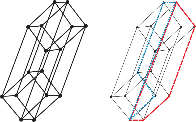
The key observation is that the projection of the 1-skeleton of hypercube can serve as a universal permuting machine: together with any configuration $P$ , it contains all other configurations obtained from $P$ by permuting the order of edges, see Figure 8.

On the one hand, an obvious advantage of this approach is that we do not remove and add bars at each step. On the other hand, a disadvantage is that we add many extra bars. Therefore, the choice between the two ways depends on the particular task.

Algorithm C

(1)

We assume that the starting and the target points are $S,\ T\in M(L)$ . We find the vertices $V_{S}$ and $V_{T}$ exactly as in Algorithm B.
(2)

Interpret the edges of $S$ numbered $1,2,...,(n-1)$ as projections of edges of the hypercube $[0,1]^{n-1}$ . The edge numbered by $n$ is then the projection of the diagonal of the hypercube. Add extra bars to incorporate $S$ to the entire projection of the hypercube, which is now treated as a bar-and-joint mechanism, see Figure 8.
(3)

The new mechanism includes also $Conv(S)$ . Now we can manipulate by $Conv(P)$ following Algorithm A. As in Algorithm B, we first bring $Conv(S)$ to the configuration labeled by $V_{S}=(I,\{1\},J).$
(4)

Next, we follow the path on the graph $\Gamma$ prescribed by Algorithm A. For each step, we manipulate with the convex configuration $Conv(P)$ which degenerates to a convex quadrilateral.
(5)

The last step from $V_{T}$ to $T$ is the same as the very first step.

References

[1] O. Aichholzer, E. D. Demaine, J. Erickson, F. Hurtado, M. Overmars, M. Soss, G. Toussaint, Reconfiguring convex polygons, Computational Geometry 20 (2001), 85-95.
[2] M. Farber and D. Schütz, Homology of planar polygon spaces, Geom. Dedicata, 125 (2007), 75-92.
[3] M. Kapovich and J. Millson, Universality theorems for configuration spaces of planar linkages, Topology, 41 (2002), 1051-1107.
[4] M. Kapovich and J. Millson, On the moduli space of polygons in the Euclidean plane, J. Diff. Geom., 42 (1995), 430-464.
[5] W. J. Lenhart, S. H. Whitesides, Reconfiguring closed polygonal chains in Euclidean $d$ -space, Discrete and Computational Geometry 13 (1995), Issue 1, 123-140.
[6] G.F. Liu, J.C. Trinkle, Complete Path Planning for Planar Closed Chains Among Point Obstacles, in: Proceedings of Robotics: Science and Systems, 2005, Cambridge, USA.
[7] G. Panina, Moduli space of planar polygonal linkage: a combinatorial description, arXiv:1209.3241
[8] J.-C. Hausmann, Controle des bras articules et transformations de Mobius. L’Enseignement Mathematique, 51 (2005) 87-115.
[9] J.-C. Hausmann and E. Rodriguez, Holonomy orbits of the snake charmer algorithm, Geometry and Topology of Manifolds, Banach Center Publications, 76 (2007)
[10] G. Khimshiashvili, Maxwell problem for polygonal linkages, Bull. Georgian Natl. Acad. Sci. 6, 2012, No. 2, 17-22.
[11] G. Panina, G. Khimshiashvili, On the area of a polygonal linkage, Doklady Akademii Nauk, Mathematics, 85, No. 1 (2012), 120-121.
[12] G. Khimshiashvili, G. Panina, and D. Siersma, Coulomb control of polygonal linkages, J. of Dynamical and Control Systems, 20, 2014, No. 4, 491-501.